Hadron diffractive production at ultrahigh energies

Abstract

Diffractive production is considered in the ultrahigh energy region where pomeron exchange amplitudes are transformed into black disk ones due to rescattering corrections. The corresponding corrections in hadron reactions $h_{1}+h_{3}\to h_{1}+h_{2}+h_{3}$ with small momenta transferred ($q^{2}_{1\to 1}\sim m^{2}/\ln^{2}s$, $q^{2}_{3\to 3}\sim m^{2}/\ln^{2}s$) are calculated in terms of the $K$-matrix technique modified for ultrahigh energies. Small values of the momenta transferred are crucial for introducing equations for amplitudes. The three-body equation for hadron diffractive production reaction $h_{1}+h_{3}\to h_{1}+h_{2}+h_{3}$ is written and solved precisely in the eikonal approach. In the black disk regime final state scattering processes do not change the shapes of amplitudes principally but dump amplitudes in a factor $\sim\frac{1}{4}$.

PACS: 13.85.Lg 13.75.Cs 14.20.Dh

1 Introduction

Recent data for diffractive production of hadrons [1, 2] demonstrate a remarkable phenomenon: an appearance of a black spot in the impact parameter presentation of the $pp$-scattering amplitude. So, one may suppose that the black disk picture starts at $\sqrt{s}\sim 10-100$ TeV. The key point is the steady growth of total and elastic cross sections up to the region $\sqrt{s}\sim 5-50$ TeV, for the preLHC data see [3]. The phenomenon of the increase of high energy cross sections was discussed for a long time. First, the power growth, $s^{\alpha}$ with $\alpha>1$, was suggested [4, 5] on the basis of the reggeon exchange notion. Then, it was shown in [6, 7, 8] that the power-type growth of scattering amplitudes with energy is dumped to $\ln^{2}s$-type within the $s$-channel unitarization. The black disk picture at ultrahigh energies is realized in the Dakhno-Nikonov model [9] for $\pi p$ and $p^{\pm}p$ collisions. The model, being QCD-motivated, takes into account the quark structure of colliding hadrons, the gluon origin of the input pomeron and the colour screening effects in collisions. The model can be considered as a realization of the Good-Walker eikonal approach [10] for a continuous set of channels.

An appropriate way for the description of the diffractive scattering data at ultrahigh energies seems to be the use of the profile function in a version of the Good-Walker approach with the Froissart bound [11] (though exceeding the Froissart bound does not violate necessarily the general constraints [12]). Examples of such descriptions can be found in [13, 14, 15, 16, 17].

The description of the recent data in terms of the Dakhno-Nikonov model and the extension of results into the ultrahigh energy region was performed in [18, 19], a short summary is given in [20]. The fit tells that the 5-50 TeV region turns out to be that where the asymptotic behaviour starts; the asymptotic regime should reveal itself definitely at $10^{2}-10^{4}$ TeV.

For the ultrahigh energy limit the black disk picture predicts a $(\ln^{2}s)$-growth for total and elastic hadron-hadron cross sections: $\sigma_{tot}\sim\ln^{2}s$ with $[\sigma_{el}/\sigma_{tot}]_{\ln s\to\infty}\to 1/2$. Further, the differential elastic cross sections depend asymptotically on transverse momenta with a relation for $\tau$-scaling: $d\sigma_{el}(\tau)/d\tau=D(\tau)$ with $\int_{0}^{\infty}d\tau D(\tau)=\sigma_{el}(s)$ and $\tau={\bf q}_{\perp}^{2}\sigma_{tot}\propto{\bf q}_{\perp}^{2}\ln^{2}s\,$ . The universal behaviour of all total and elastic cross sections is the consequence of the universality of the colliding disk structure, or the structure of parton clouds at ultrahigh energy. The diffractive dissociation processes are increasing at asymptotic energies ($\sigma_{D}\propto\ln{s}$, $\sigma_{DD}\propto\ln{s}$) but their relative contribution tends to zero ($\sigma_{D}/\sigma_{tot}\to 0$, $\sigma_{DD}/\sigma_{tot}\to 0$).

The universal character of the black disks and the $\tau$-scaling phenomenon open a path for consideration of hadron productions in diffractive collisions. The simplest process of this type is the diffractive production of hadron shower, $p+p\to M_{X}+p$, the cross section of this process at moderately high energies is usually modeled by three-pomeron diagrams. More complicated for consideration is the process of diffractive scattering with the production of a third particle, $pp\to php$, with large pair energies ($s_{ph}\sim s_{hp}\sim m\sqrt{s}$) and small momenta transferred to protons (${\bf q}_{p\perp}^{2}\sim m^{2}/\ln^{2}s$). This process is the subject of our studies in this paper (see also Fig. 1).

The eikonal approach for the black disk picture means a composite structure of a colliding object: a standard example is the interaction of a fast particle with a nucleus when multiple elastic scatterings on nucleons of a nucleus give $\eta\to 0$ for the $hA$-amplitude. Time ordering of scatterings is a necessary step in the consideration of such processes, and it results in the eikonal approach. Partons, being hadron components, form the inner structure of hadrons thus justifying the use of the eikonal approach for hadron collisions.

Using the $K$-matrix method, or the dispersion relation N/D-approach, we get an appropriate way for the consideration of three-particle production processes [21]. Therefore, the first problem we face here is the extension of these techniques to ultrahigh energies. In Chapter 2 we consider examples of diagrams for the production of three hadrons with very small momenta transferred, $q^{2}\sim m^{2}/\ln^{2}s$. The examples demonstrate us specific features in the formulation of the eikonal approach with the $K$-matrix. In Chapter 3 in the framework of the developed technique we write in the impact parameter space a system of equations which determines the diffractive production amplitude in hadron-hadron collisions at ultrahigh energies; we solve the equation. The hypothesis about the black disk structure of the two-particle interaction amplitude allows an easy calculation of screening effects inherent to ultrahigh energies, results of such calculations are presented in Chapter 4.

In the Conclusion we summarize the results.

2 Three particle production amplitude and initial/final state interactions

At ultrahigh energies the initial state and final state rescatterings are to be taken into account: the growth of total and elastic cross sections definitely tells us that the effect of rescatterings is not small. Here we consider examples of such processes using the impact parameter representation. But first we recall the corresponding presentation for the elastic scattering amplitude.

For the two-particle scattering amplitude the standard determination of the profile function $T(b,\xi)$ in the impact parameter space, ${\bf b}$, can be written as:

$$4\pi\frac{d\sigma_{el}}{dq^{2}_{\perp}}=A^{2}(q^{2}_{\perp},\xi),\quad A(q^{2}_{\perp},\xi)=\int d^{2}b\;e^{i{\bf b}{\bf q}_{\perp}}T(b,\xi)\,,$$

$$T(b,\xi)=1-e^{-\frac{1}{2}\chi(b,\xi)}=1-\eta(b,\xi)\,e^{2i\delta(b,\xi)}=\frac{-2iK(b,\xi)}{1-iK(b,\xi)},$$

$$b=|{\bf b}|,\quad\xi=\ln s,$$

where the profile function is presented in terms of the optical density $\chi(b,\xi)$, the inelasticity parameter and the phase shift, $\eta(b,\xi)$ and $\delta(b,\xi)$, and using the $K$-matrix approach (the function $K(b,\xi)$ for the multichannel case is complex valued).

Below we calculate explicitly examples of diagrams for the production of three particles using the $K$-matrix technique in the ${\bf b}$-space.

2.1 Feynman diagram technique and eikonal approach

Let us consider the amplitude of the Fig. 1c,d type (last interaction in 23-channel). The Feynman integral for the loop related to the intermediate $2^{\prime}3^{\prime}$-state reads:

$$\int\frac{d^{4}k_{2^{\prime}}}{(2\pi)^{4}i}\;A_{2\to 3}\left(k_{1},k_{2^{\prime}},k_{3^{\prime}}\right)\frac{1}{(m^{2}-k^{2}_{2^{\prime}}-i0)(m^{2}-k^{2}_{3^{\prime}}-i0)}\;A_{2\to 2}\left(k_{2^{\prime}},k_{3^{\prime}}\right)\,.$$ (1)

The key point is that interactions at ultrahigh energies turn out to be effectively instantaneous. This is the result of shrinking of the diffractive cones (the effect of the $\tau$-scaling): the substantial regions of integration over momenta transferred are small, of the order of ${\bf q}^{2}\sim m^{2}/\xi^{2}$ with $\xi\equiv\ln s>>1.$

             

             

Figure 1: Input diagram for diffractive production (a) and diagrams with rescatterings in initial and final states: the last interactions in 12-channel (b), in 23-channel (c) and 13-channel (d).

It is convenient to consider three-particle production processes in the cm-system where the initial particle momenta are determined as $p_{1}=(p_{0},{\bf p}_{\perp},p_{z})\simeq(p+m^{2}/2p,0,p)$ and $p_{3}\simeq(p+m^{2}/2p,0,-p)$. Therefore, in this system we have the following relations:

$${\bf k}_{1\perp}+{\bf k}_{2^{\prime}\perp}+{\bf k}_{3^{\prime}\perp}=0,\quad{\bf k}_{1\perp}+{\bf k}_{2\perp}+{\bf k}_{3\perp}=0,$$ (2)

$$m^{2}_{2^{\prime}\perp}=m^{2}+{\bf k}^{2}_{2^{\prime}\perp},\quad q^{2}_{1}=(p_{1}-k_{1})^{2}\simeq-{\bf k}^{2}_{1\perp},$$

$$q^{2}_{3^{\prime}}=(p_{3}-k_{3^{\prime}})^{2}\simeq-{\bf k}^{2}_{3^{\prime}\perp},\quad q^{2}_{3^{\prime}3}=(k_{3^{\prime}}-k_{3})^{2}\simeq-({\bf k}_{3\perp}-{\bf k}_{3^{\prime}\perp})^{2}\,.$$

The integral (1) within this kinematics is written as:

$$\int\frac{dk_{2^{\prime}}^{(+)}dk_{2^{\prime}}^{(-)}d^{2}{k}_{2^{\prime}\perp}}{2i(2\pi)^{4}}\;\frac{A_{2\to 3}\left(k_{1},k_{2^{\prime}},k_{3^{\prime}}\right)A_{2\to 2}\left(k_{2^{\prime}},k_{3^{\prime}}\right)}{\left(k_{2^{\prime}}^{(+)}k_{2^{\prime}}^{(-)}-(m^{2}+{\bf k}^{2}_{2^{\prime}\perp})+i0\right)\left(k_{3^{\prime}}^{(+)}k_{3^{\prime}}^{(-)}-(m^{2}+{\bf k}^{2}_{3^{\prime}\perp})+i0\right)}\,.$$ (3)

where $k_{2^{\prime}}^{(\pm)}=k_{2^{\prime}0}\pm k_{2^{\prime}z}$ and $k_{3^{\prime}}^{(\pm)}=k_{3^{\prime}0}\pm k_{3^{\prime}z}$. The eikonal approach corresponds to the mass-on-shell calculation of loop diagrams. It can be seen when considering the $K$-matrix elements. The $K$-matrix function $(-i)K(b,\xi)$ of a scattering amplitude is real for the black disk regime. This means that the imaginary parts in loop diagrams are dominant. For the rescattering diagrams of the type given in Fig. 1, it is realized by the replacement:

$$\left[(m^{2}-k^{2}_{2^{\prime}}-i0)(m^{2}-k^{2}_{3^{\prime}}-i0)\right]^{-1}\to-2\pi^{2}\delta(m^{2}-k^{2}_{2^{\prime}})\delta(m^{2}-k^{2}_{3^{\prime}})$$

$$= -2\pi^{2}\delta\left(k_{2^{\prime}}^{(+)}k_{2^{\prime}}^{(-)}-(m^{2}+{\bf k}^{2}_{2^{\prime}\perp})\right)\delta\left(k_{3^{\prime}}^{(+)}k_{3^{\prime}}^{(-)}-(m^{2}+{\bf k}^{2}_{3^{\prime}\perp})\right)\;.$$

Then the amplitude (1) reads (below we skip the index $\perp$):

$$\int\frac{d^{2}{k}_{2^{\prime}}}{(2\pi)^{2}}\frac{i}{4s_{23}}\left[A_{2\to 3}\left(k_{1},k_{2^{\prime}},k_{3^{\prime}}\right)A_{2\to 2}\left(k_{2^{\prime}},k_{3^{\prime}}\right)\right]^{k^{2}_{2^{\prime}}=m^{2}}_{k^{2}_{3^{\prime}}=m^{2}}\;.$$

For mass-on-shell amplitudes we introduce the notation:

$$\left[A_{2\to 3}\left(k_{1},k_{2^{\prime}},k_{3^{\prime}}\right)\right]^{k^{2}_{2^{\prime}}=m^{2}}_{k^{2}_{3^{\prime}}=m^{2}}\equiv A^{(23)}\left({\bf k}^{2}_{1},\xi_{12};\;{\bf k}^{2}_{3^{\prime}},\xi_{23}\right)\,,$$ (5)

$$\frac{1}{4s_{23}}\left[A_{2\to 2}\left(k_{2^{\prime}},k_{3^{\prime}}\right)\right]^{k^{2}_{2^{\prime}}=m^{2}}_{k^{2}_{3^{\prime}}=m^{2}}\equiv K_{2\to 2}\left(({\bf k}_{3^{\prime}}-{\bf k}_{3})^{2},\xi_{23}\right)\,,$$

where $K\left(({\bf k}_{3^{\prime}}-{\bf k}_{3})^{2},\xi_{23}\right)$ is the $K$-matrix function in momentum representation, $\xi_{23}=\ln s_{23}$ and $s_{23}=(k_{2}+k_{3})^{2}$. After changing integration $d^{2}{\bf k}_{2^{\prime}}\to d^{2}{\bf k}_{3^{\prime}}$, we, finally, write for Eq. (1):

$$\int\frac{d^{2}{k}_{3^{\prime}}}{(2\pi)^{2}}A^{(23)}\left({\bf k}^{2}_{1},\xi_{12};\;{\bf k}^{2}_{3^{\prime}},\xi_{23}\right)\;iK\left(({\bf k}_{3^{\prime}}-{\bf k}_{3})^{2},\xi_{23}\right)\,.$$ (6)

The procedure of calculating mass-on-shell rescatterings given here corresponds exactly to the eikonal approach used in [9, 18, 19]. The Fourier transform of Eq. (6) (the operator reads as $\int d^{2}{k}_{1}/(2\pi)^{2}\exp{\left(-i{\bf k}_{1}{\bf b}_{1}\right)}\int d^{2}{k}_{3}/(2\pi)^{2}\exp{\left(-i{\bf k}_{3}{\bf b}_{3}\right)}$) gives us the amplitude in the impact parameter space.

2.2 Amplitudes of initial and final state rescatterings in the impact parameter space

We continue to consider examples of diagrams with initial and final state screenings but in terms of the $K$-matrix. The best way for that is to use the impact parameter representation. For the scattering amplitude we write $T(b,\xi)=\left(-2iK(b,\xi)\right)/\left(1-iK(b,\xi)\right)$, for production amplitudes we should use the corresponding Fourier transforms.

2.2.1 Initial state rescatterings

The bare amplitude for the production of three particles and its Fourier transform (see Fig. 1a) are written as:

$$\phi_{0}({\bf k}^{2}_{1},\xi_{12};\;{\bf k}^{2}_{3},\xi_{23})=\int d^{2}{b}_{1}d^{2}{b}_{3}f_{0}(b_{1},\xi_{12}\;;b_{3}\,,\xi_{23})\exp\left(i{\bf k}_{1}{\bf b}_{1}+i{\bf k}_{3}{\bf b}_{3}\right).$$ (7)

We use the same notations for the bare amplitude and its Fourier transform supposing that do not lead to misunderstanding.

The rescattering in the initial state gives an additional factor in the impact parameter space

$$\phi_{1}({\bf k}^{2}_{1},\xi_{12};\;{\bf k}^{2}_{3},\xi_{23}) = \int d^{2}{b}_{1}d^{2}{b}_{3}\;iK(b,\xi)f_{0}(b_{1},\xi_{12}\;;b_{3}\,,\xi_{23})\exp\left(i{\bf k}_{1}{\bf b}_{1}+i{\bf k}_{3}{\bf b}_{3}\right),$$

$$\xi = \xi_{12}+\xi_{23},\quad{\bf b}={\bf b}_{1}+{\bf b}_{3},$$ (8)

two rescatterings result in $\left[iK(b,\xi)\right]^{2}$ and so on. The summation of all terms $\sum\limits_{n=0,1,2,...}\phi_{n}$ generates the standard $K$-matrix factor $\left[1-iK(b,\xi)\right]^{-1}$, and we write for the input term corrected by taking into account the initial state interactions:

$$\phi({\bf k}^{2}_{1},\xi_{12};\;{\bf k}^{2}_{3},\xi_{23})=\int d^{2}{b}_{1}d^{2}{b}_{3}\;\frac{1}{1-iK(b,\xi)}f_{0}(b_{1},\xi_{12}\;;b_{3}\,,\xi_{23})\exp\left(i{\bf k}_{1}{\bf b}_{1}+i{\bf k}_{3}{\bf b}_{3}\right),$$ (9)

Below we use the notation

$$f(b_{1},\xi_{12}\;;b_{3}\,,\xi_{23})=\frac{1}{1-iK(b,\xi)}f_{0}(b_{1},\xi_{12}\;;b_{3}\,,\xi_{23})$$ (10)

The factor $\left[1-iK(b,\xi)\right]^{-1}$ is universal for all terms of the amplitude. Hence, it should be introduced into all components of the amplitude. Below, without special emphasizes, we presume that it is done.

2.2.2 Input term $\phi({\bf k}^{2}_{1},\xi_{12};\;{\bf k}^{2}_{3},\xi_{23})$ and final state rescatterings

First, we consider rescatterings in 23- and 12-channels. The input term with the corresponding rescatterings can be written as:

$$\phi^{(23)}({\bf k}^{2}_{1},\xi_{12};\;{\bf k}^{2}_{3},\xi_{23})=\int d^{2}{b}_{1}d^{2}{b}_{3}f^{(23)}(b_{1},\xi_{12}\;;b_{3}\,,\xi_{23})\exp\left(i{\bf k}_{1}{\bf b}_{1}+i{\bf k}_{3}{\bf b}_{3}\right),$$

$$\phi^{(12)}({\bf k}^{2}_{3},\xi_{23};\;{\bf k}^{2}_{1},\xi_{12})=\int d^{2}{b}_{1}d^{2}{b}_{3}f^{(12)}(b_{3}\,,\xi_{23}\;;b_{1},\xi_{12})\exp\left(i{\bf k}_{1}{\bf b}_{1}+i{\bf k}_{3}{\bf b}_{3}\right),$$ (11)

where

$$f^{(23)}(b_{1},\xi_{12}\;;b_{3}\,,\xi_{23}) = f(b_{1},\xi_{12}\;;b_{3}\,,\xi_{23})\frac{iK(b_{3},\xi_{23})}{1-iK(b_{3},\xi_{23})}$$

$$\equiv f(b_{1},\xi_{12}\;;b_{3}\,,\xi_{23})\;a(b_{3},\xi_{23}),$$

$$f^{(12)}(b_{3}\,,\xi_{23}\;;b_{1},\xi_{12}) = f(b_{1},\xi_{12}\;;b_{3}\,,\xi_{23})\frac{iK(b_{1},\xi_{12})}{1-iK(b_{1},\xi_{12})}$$ (12)

$$\equiv f(b_{1},\xi_{12}\;;b_{3}\,,\xi_{23})\;a(b_{1},\xi_{12})\,.$$

Here we introduce a short notation for the two-particle scattering amplitude.

Rescatterings in the 13-channel give us the input term $f^{(13)}$. Since here ${\bf k}_{1}+{\bf k}_{3}={\bf k}_{1^{\prime}}+{\bf k}_{3^{\prime}}$, it is convenient to use the equation for rescatterings in a somewhat modified form:

$$\phi^{(13)}({\bf k}^{2}_{1},\xi_{12};\;{\bf k}^{2}_{3},\xi_{23}) = \int\frac{d^{2}{k}_{3^{\prime}}d^{2}{k}_{1^{\prime}}}{(2\pi)^{2}}\;\delta\left({\bf k}_{1}+{\bf k}_{3}-{\bf k}_{1^{\prime}}-{\bf k}_{3^{\prime}}\right)$$

$$\times \phi({\bf k}^{2}_{1^{\prime}},\xi_{12};\;{\bf k}^{2}_{3^{\prime}},\xi_{23})\;iK\left(({\bf k}_{3^{\prime}_{\perp}}-{\bf k}_{3_{\perp}})^{2},\xi_{13}\right)\,.$$

The transformation of this equality into the impact parameter space leads to

$$f^{(13)}_{1}(b_{1}\,,\xi_{12}\;;b_{3},\xi_{23}\;;|{\bf b}_{1}+{\bf b}_{3}|\,,\xi_{13}) = f(b_{1},\xi_{12}\;;b_{3}\,,\xi_{23})\;iK(|{\bf b}_{1}+{\bf b}_{3}|\,,\xi_{13}),$$

$$\xi_{13} \simeq \xi=\xi_{12}+\xi_{23}\,.$$ (14)

Performing a summation over the complete set of rescattering diagrams in the 13-channel, $\sum\limits_{n=1,2,3...}f^{(13)}_{n}$, we write:

$$f^{(13)}(b_{1}\,,\xi_{12}\;;b_{3},\xi_{23}\;;|{\bf b}_{1}+{\bf b}_{3}|\,,\xi) = f(b_{1},\xi_{12}\;;b_{3}\,,\xi_{23})\frac{iK(|{\bf b}_{1}+{\bf b}_{3}|\,,\xi)}{1-iK(|{\bf b}_{1}+{\bf b}_{3}|\,,\xi)}$$

$$\equiv f(b_{1},\xi_{12}\;;b_{3}\,,\xi_{23})\;a\left(|{\bf b}_{1}+{\bf b}_{3}|\,,\xi\right).$$

Formulae (12), (2.2.2) give us the pattern for writing other diagrams with final state rescatterings.

Figure 2: Four terms for a three particle production amplitude: the input term without final state rescatterings (a), and the terms with rescatterings in the $23$-channel (b), in the $12$-channel (c), and the $13$-channel (d).

3 System of equations for the production amplitude

Figure 3: Diagrams with final state rescatterings in the channels 23,12 and 13 - figures $a$, $b$ and $c$ correspondingly. Equalities are graphical realizations of equations for the amplitudes $A^{(ij)}$.

We present the amplitude as a sum of four terms:
(i) input term $f(b_{1},\xi_{12}\;;b_{3}\,,\xi_{23})$ without final state interactions,
(ii) terms with interactions in final states, that are $12$-, $23$-states and $13$-state with corresponding amplitudes $A^{(12)}(b_{1},\xi_{12}\;;b_{3}\,,\xi_{23})$, $A^{(23)}(b_{1},\xi_{12}\;;b_{3}\,,\xi_{23})$, and $A^{(13)}(b_{1},\xi_{12}\;;b_{3}\,,\xi_{23};|{\bf b}_{1}+{\bf b}_{3}|\,,\xi)$.
The index $(ij)$ shows the channel in which the last interaction in the final state takes place. We suppose that initial state interactions in the amplitudes $f$ and $A^{(ij)}$ are taken into account. Then, the total amplitude, see Fig. 2, is written as follows:

$$A^{(tot)}_{2\to 3} = f(b_{1},\xi_{12}\;;b_{3}\,,\xi_{23})+A^{(12)}(b_{1},\xi_{12}\;;b_{3}\,,\xi_{23})$$ (16)

$$+ A^{(23)}(b_{1},\xi_{12}\;;b_{3}\,,\xi_{23})+A^{(13)}(b_{1},\xi_{12}\;;b_{3}\,,\xi_{23};|{\bf b}_{1}+{\bf b}_{3}|,\,\xi).$$

The equations for $A^{(ij)}$ are shown in Fig. 3, they are written as:

$$A^{(23)}(b_{1},\xi_{12}\;;b_{3}\,,\xi_{23})=f(b_{1},\xi_{12}\;;b_{3}\,,\xi_{23})\;a_{23}(b_{3},\xi_{23})$$ (17)

$$+ A^{(12)}(b_{1},\xi_{12}\;;b_{3}\,,\xi_{23})\;a_{23}(b_{23},\xi_{23})+A^{(13)}(b_{1},\xi_{12}\;;b_{3}\,,\xi_{23};|{\bf b}_{1}+{\bf b}_{3}|,\,\xi)\;a_{23}(b_{23},\xi_{23}),$$

$$A^{(12)}(b_{1},\xi_{12}\;;b_{3}\,,\xi_{23})=f(b_{1},\xi_{12}\;;b_{3}\,,\xi_{23})\;a_{12}(b_{1},\xi_{12})$$

$$+ A^{(23)}(b_{1},\xi_{12}\;;b_{3}\,,\xi_{23})a_{12}(b_{1},\xi_{12})+A^{(13)}(b_{1},\xi_{12}\;;b_{3}\,,\xi_{23};|{\bf b}_{1}+{\bf b}_{3}|,\,\xi)\;a_{12}(b_{1},\xi_{12}),$$

$$A^{(13)}(b_{1},\xi_{12}\;;b_{3}\,,\xi_{23};|{\bf b}_{1}+{\bf b}_{3}|,\,\xi)=f(b_{1},\xi_{12}\;;b_{3}\,,\xi_{23})\;a_{13}(|{\bf b}_{1}+{\bf b}_{3}|,\,\xi)$$

$$+ A^{(12)}(b_{1},\xi_{12}\;;b_{3}\,,\xi_{23})\;a_{13}(|{\bf b}_{1}+{\bf b}_{3}|,\,\xi)+A^{(23)}(b_{1},\xi_{12}\;;b_{3}\,,\xi_{23})\;a_{13}(|{\bf b}_{1}+{\bf b}_{3}|,\,\xi).$$

Let us recall that the two-particle amplitudes, $a_{ij}$, are introduced in Eq. (12), namely:

$$a_{23}\equiv a_{23}(\xi_{23},b_{23})=\frac{iK(b_{3},\xi_{23})}{1-iK(b_{3},\xi_{23})}\;,$$ (18)

$$a_{12}\equiv a_{12}(b_{1},\xi_{12})=\frac{iK(b_{1},\xi_{12})}{1-iK(b_{1},\xi_{12})}\;,$$

$$a_{13}\equiv a_{13}(|{\bf b}_{1}+{\bf b}_{3}|,\,\xi)=\frac{iK(|{\bf b}_{1}+{\bf b}_{3}|,\,\xi)}{1-iK(|{\bf b}_{1}+{\bf b}_{3}|,\,\xi)}\;.$$

Amplitudes $A^{(23)}$ and $A^{(12)}$ differ only by the permutation of indices $1\rightleftharpoons 3$. In a short form Eq. (17) reads:

$$A^{(23)}=fa_{23}+A^{(12)}a_{23}+A^{(13)}a_{23},$$

$$A^{(12)}=fa_{12}+A^{(23)}a_{12}+A^{(13)}a_{12},$$

$$A^{(13)}=fa_{13}+A^{(12)}a_{13}+A^{(23)}a_{13}.$$ (19)

The equations give us

$$A^{(12)}=f\frac{1+a_{13}+a_{23}+a_{23}a_{13}}{1-a_{12}a_{23}-a_{12}a_{13}-a_{23}a_{13}-2a_{12}a_{23}a_{13}}\,a_{12},$$

$$A^{(23)}=f\frac{1+a_{13}+a_{12}+a_{12}a_{13}}{1-a_{23}a_{12}-a_{23}a_{13}-a_{12}a_{13}-2a_{12}a_{23}a_{13}}\,a_{23},$$ (20)

$$A^{(13)}=f\frac{1+a_{12}+a_{23}+a_{23}a_{12}}{1-a_{23}a_{12}-a_{23}a_{13}-a_{12}a_{13}-2a_{12}a_{23}a_{13}}\,a_{13},$$

with

$$f=\frac{1}{1-iK(b,\xi)}f_{0},\qquad\xi=\xi_{12}+\xi_{23},\quad{\bf b}={\bf b}_{1}+{\bf b}_{3}\,.$$ (21)

The input term $f_{0}$ depends also on ${\bf b}_{j}$ and $\xi_{ij}$. At moderately high energies it is a two-pomeron term, at ultrahigh energies it can be a two-disk term. So, for the two-pomeron term we write correspondingly in the momentum and impact parameter spaces:

$${\rm{\bf k}-space:} \quad f_{0}=g_{2\to 3}\cdot ie^{-i\frac{\pi}{2}\Delta}\exp{\left[\Delta\xi_{12}-\alpha^{\prime}\xi_{12}{\bf k}^{2}_{1}\right]}\cdot ie^{-i\Delta\frac{\pi}{2}}exp{\left[\Delta\xi_{23}-\alpha^{\prime}\xi_{23}{\bf k}^{2}_{3}\right]}\,,$$

$${\rm{\bf b}-space:} \quad f_{0}=g_{2\to 3}\cdot\frac{ie^{-i\frac{\pi}{2}\Delta+\Delta\xi_{12}}}{4\pi\alpha^{\prime}\xi_{12}}\exp\left[-\frac{{\bf b}^{2}_{1}}{4\alpha^{\prime}\xi_{12}}\right]\frac{ie^{-i\frac{\pi}{2}\Delta+\Delta\xi_{23}}}{4\pi\alpha^{\prime}\xi_{23}}\exp\left[-\frac{{\bf b}^{2}_{3}}{4\alpha^{\prime}\xi_{23}}\right]\,.$$ (22)

In the black disk mode the input term reads:

$${\rm{\bf k}-space:} f_{0}=g_{2\to 3}\cdot iA({\bf k}^{2}_{1},\xi_{12})\;iA({\bf k}^{2}_{3},\xi_{23})\,,$$

$${\rm{\bf b}-space:} f_{0}=g_{2\to 3}\cdot iT(b_{1},\xi_{12})\;iT(b_{3},\xi_{23})\,$$ (23)

with $A({\bf k}^{2},\xi)$, $T(b,\xi)$ determined in Eq. (2).

In the black disk mode the amplitudes $a_{ij}$ behave as $a_{ij}\to-\frac{1}{2}$ in the region $b<R_{black\;disk}\simeq R_{0}\ln s$ and $a_{ij}\to\;0$ at large distances (beyond the black disk area). Therefore the denominator of Eq. (3) is non-zero, and that results in a unique solution.

Figure 4: The $K$-matrix function $(-i)K(b,\xi)$ for the $pp$ scattering amplitude at $\sqrt{s}=1$, $10$ TeV is obtained by the fit of existing data [1, 2, 3]. The curves at $\sqrt{s}=10^{n}$ TeV at $n\geq 2$ show a continuation of the fit results [18, 19] to ultrahigh energies in terms of the black disk picture, here at $b<R_{black\;disk}\simeq R_{0}\ln s$ one has $(-i)K(b,\xi)\to 1$.

3.1 Black disk mode and numerical solution of the three-body equation

For numerical calculations of $f$, $A^{(ij)}$ and $A^{(tot)}=f+\sum A^{(ij)}$ we use the Dakhno-Nikonov model [9] with fit results for $\left(-iK(b,\xi)\right)$ obtained in [18, 19].

In Fig. 4a we show the profile functions $T(b,\xi)$ found in the fit of data [1, 2, 3]. So, we can regard the profile functions at $\sqrt{s}=1,10,100$ TeV as those restored by the data, while $T(b,\xi)$ at $\sqrt{s}=10^{n},\;n>2$ are asymptotic values for the black disk regime. The corresponding $-iK(b,\xi)$ are shown in Fig. 4b. The numerical calculation of $f$, $A^{ij}$, $A^{tot}$ are performed using these $\left(-iK(b,\xi)\right)$, the results are demonstrated in Figs. 5 and 6.

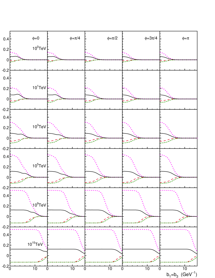
Figure 5: Black disk mode: Production amplitudes in impact parameter space for colliding energies $\sqrt{s}=1,10,10^{3},10^{5},10^{9},10^{15}$ TeV at $b_{1}=b_{3}$ and $\xi_{12}=\xi_{23}=\xi/2$, $\phi$ is the angle between ${\bf b}_{1}$ and ${\bf b}_{3}$: $A^{(12)}=A^{(23)}$ are red dashed curves, $A^{(13)}$ are green dot-dashed curves, $f$ are pink dotted curves, $A^{(tot)}$ are black solid curves, see (16), (3), (3).

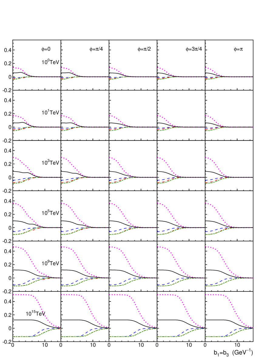
Figure 6: Black disk mode: Production amplitudes in impact parameter space for colliding energies $\sqrt{s}=1,10,10^{3},10^{5},10^{9},10^{15}$ TeV at $b_{1}=b_{3}$ and $\xi_{12}=\xi/3$, $\xi_{23}=2/3\;\xi$, $\phi$ is the angle between ${\bf b}_{1}$ and ${\bf b}_{3}$: $A^{(12)}=A^{(23)}$ are red dashed curves, $A^{(13)}$ are green dot-dashed curves, $f$ are pink dotted curves, $A^{(tot)}$ are black solid curves, see (16), (3), (3).

The comparison of the input amplitude $f$ with $A^{(tot)}$ demonstrates that final state scattering corrections do not change principally the shape of $A^{(tot)}$ but dump the amplitude in a factor $\sim\frac{1}{4}$.

4 Conclusion

The diffractive scattering amplitudes are growing with energy thus causing the necessity to take into account rescatterings that result in screening effects. In this paper we calculate these effects in the framework of modified $K$-matrix technique for eikonal amplitudes. Corresponding calculations of screening effects in diffractive production processes are performed in the impact parameter space.

The key point of the approach is a shrinkage of diffractive cones in hadron reactions at ultrahigh energies. The shrinkage of cones with energy growth demonstrates us the effective suppression of the $t$-channel singularities that allow us to use quasi-instantaneous interactions. Being more detailed, one can suppose that the long-ranged component of interaction is determined by a cloud of partons which have universal characteristics and properties. These long-ranged interactions are quasi-instantaneous, thus opening possibilities to a standard treatment of the multiparticle production processes; examples of such considerations can be found in [21]. The generalization to other ultrahigh energy diffractive production processes is possible within the developed technique.

The authors thank Y.I. Azimov, J. Nyiri and M.G. Ryskin for useful discussions and comments. The work was supported by grants RFBR-13-02-00425 and RSGSS-4801.2012.2.

References

• [1] G. Latino for the TOTEM collaboration, Summary of Physics Results from the TOTEM Experiment, arXiv:1302.2098(2013) [hep-ph].
• [2] Pierre Auger Collaboration (P. Abreu et al.), Phys. Rev. Lett. 109, 062002 (2012).
• [3] UA4 Collaboration, Phys. Lett. B147 , 385 (1984);
UA4/2 Collaboration, Phys. Lett. B316, 448 (1993);
UA1 Collaboration, Phys. Lett. B128, 336 (1982);
E710 Collaboration, Phys. Lett. B247, 127 (1990);
CDF Collaboration, Phys. Rev. D50, 5518 (1994).
• [4] A.B. Kaidalov and K.A. Ter-Martirosyan, Sov. J. Nucl. Phys. 39, 979 (1984).
• [5] A. Donnachie and P.V. Landshoff, Nucl. Phys. B231, 189 (1984).
• [6] T.K. Gaisser and T. Stanev, Phys. Lett., B219, 375, 1989.
• [7] M. Block, F. Halzen and B. Margolis, Phys. Lett., B252, 481, 1990.
• [8] R.S. Fletcher, Phys. Rev. D46, 187, 1992.
• [9] L.G. Dakhno and V.A. Nikonov, Eur.Phys.J. A8, 209 (1999).
• [10] M.L. Good, W.D. Walker, Phys. Rev. 120, 1857 (1960).
• [11] M. Froissart, Phys. Rev. 123, 1053 (1961).
• [12] Y.I. Azimov, Phys. Rev. D84, 056012 (2011);
arXiv:1208.4304(2012) [hep-ph].
• [13] F. Halzen, K. Igi, M. Ishida and C.S. Kim, Phys. Rev. D85, 074020 (2012); arXiv:1110.1479V2(2012) [hep-ph].
• [14] V. Uzhinsky and A. Galoyan, arXiv:1111.4984v5(2012) [hep-ph].
• [15] M.G. Ryskin, A.D. Martin and V.A. Khoze, Eur.Phys.J. C72, 1937(2012); arXiv:1201.6298v2(2012) [hep-ph].
• [16] I.M. Dremin, V.A. Nechitailo, Phys. Rev. D85, 074009 (2012); arXiv:1202.2016 (2012) [hep-ph].
• [17] M.M. Block and F. Halzen, Phys. Rev. D86, 0501504 (2013); arXiv:1208.4086v1 (2012) [hep-ph].
• [18] V.V. Anisovich, K.V. Nikonov, and V.A. Nikonov, Phys. Rev. D88, 014039 (2013); [arXiv:1306.1735 (hep-ph)].
• [19] V.V. Anisovich, V.A. Nikonov, and J. Nyiri, Phys. Rev. D88, 014039(2013); [arXiv:1310.2839 (hep-ph)].
• [20] V.V. Anisovich, K.V. Nikonov, V.A. Nikonov and J. Nyiri, Int.J.Mod.Phys. A29, 1450096 (2014); arXiv:1404.1904 (hep-ph).
• [21] A.V. Anisovich, V.V. Anisovich, M.A. Matveev, V.A. Nikonov, J. Nyiri, A.V. Sarantsev Three-particle physics and dispersion relation theory, World Scientific, Singapore (2013).