Disk Radii and Grain Sizes in Herschel-Resolved Debris Disks

Abstract

The radii of debris disks and the sizes of their dust grains are important tracers of the planetesimal formation mechanisms and physical processes operating in these systems. Here we use a representative sample of 34 debris disks resolved in various Herschel Space Observatory programs to constrain the disk radii and the size distribution of their dust. While we modeled disks with both warm and cold components, and identified warm inner disks around about two-thirds of the stars, we focus our analysis only on the cold outer disks, i.e. Kuiper-belt analogs. We derive the disk radii from the resolved images and find a large dispersion for host stars of any spectral class, but no significant trend with the stellar luminosity. This argues against ice lines as a dominant player in setting the debris disk sizes, since the ice line location varies with the luminosity of the central star. Fixing the disk radii to those inferred from the resolved images, we model the spectral energy distribution to determine the dust temperature and the grain size distribution for each target. While the dust temperature systematically increases towards earlier spectral types, the ratio of the dust temperature to the blackbody temperature at the disk radius decreases with the stellar luminosity. This is explained by a clear trend of typical sizes increasing towards more luminous stars. The typical grain sizes are compared to the radiation pressure blowout limit $s_{\mathrm{blow}}$ that is proportional to the stellar luminosity-to-mass ratio and thus also increases towards earlier spectral classes. The grain sizes in the disks of G- to A-stars are inferred to be several times $s_{\mathrm{blow}}$ at all stellar luminosities, in agreement with collisional models of debris disks. The sizes, measured in the units of $s_{\mathrm{blow}}$, appear to decrease with the luminosity, which may be suggestive of the disk’s stirring level increasing towards earlier-type stars. The dust opacity index $\beta$ ranges between zero and two, and the size distribution index $q$ varies between three and five for all the disks in the sample.

1. Introduction

Protoplanetary disks are known to exhibit broad, smooth radial profiles (Williams & Cieza 2011). However, many of their successors, debris disks, have most of the material confined to one or more distinct belts (Matthews et al. 2014b). The evidence comes from the resolved images of prominent debris disks such as that of Fomalhaut (Acke et al. 2012; Boley et al. 2012), HD 181327 (Lebreton et al. 2012) or 49 Cet (Roberge et al. 2013), and from the spectral energy distributions (SEDs) of unresolved disks that are fitted reasonably well by assuming one or two narrow dust rings at distinct locations (e.g. Morales et al. 2009, 2011; Donaldson et al. 2013; Ballering et al. 2013; Chen et al. 2014).

Observation of debris rings at specific locations around the star implies that planetesimals were able to form there by one or another mechanism (Johansen et al. 2014), or that they formed elsewhere and were moved to their current locations by migration processes or planetary scattering (Raymond et al. 2011). For the rings to be seen, it is also necessary that those regions are dynamically stable against planetary perturbations for a significant fraction of the lifetime of the central star, and that planetesimal belts retained much of their mass despite collisional depletion. Furthermore, the planetesimals at these locations have to be sufficiently excited dynamically (Wyatt 2008), either by neighboring planets (Mustill & Wyatt 2009) or embedded perturbers (Kenyon & Bromley 2008), to make planetesimal collisions destructive and to enable production of visible debris dust. It is likely that the radii of debris rings are set by planets that clear up their inner regions (Kennedy & Wyatt 2010) and may also be solely or partly responsible for triggering the collisional cascade in the debris zone. Alternatively, the debris zones may mark the locations at which planetesimals can most efficiently form. Either way, it is indisputable that the radii of debris disks bear valuable information on planetesimals and planets and their formation processes.

Another important diagnostic of debris disks is the size distribution of their dust. It reflects an interplay between grain-grain collisions, radiation pressure, various transport processes, as well as mechanisms that lead to modification of dust grains (Wyatt et al. 2011).

An essential theoretical expectation is that in the disks around solar- or earlier-type stars, the dominant grain size is $s_{\mathrm{min}}\approx bs_{\mathrm{blow}}$, where $s_{\mathrm{blow}}$ is the blowout size, below which the grains are expelled by direct radiation pressure, and $b$ is a numerical factor. The latter depends, in particular, on the dynamical excitation of dust-producing planetesimals in the disk. For collisionally active disks, collisional simulations suggest $b\sim 2$ (e.g. Krivov et al. 2006; Thébault & Augereau 2007). However, for dynamically cold disks with planetesimals in low-eccentricity, low-inclination orbits, $b$ can be much larger (Thébault & Wu 2008; Krivov et al. 2013). For instance, Löhne et al. (2012) infer $b\approx 8$ for the disk around HD 207129 (Marshall et al. 2011). Around late-type stars, radiation pressure may be too weak to eliminate grains at all sizes, so that $s_{\mathrm{min}}$ should be set by size-dependent transport mechanisms such as the Poynting-Robertson (P-R) force (see, e.g., Kuchner & Stark 2010; Vitense et al. 2010; Wyatt et al. 2011) or stellar wind drag (Plavchan et al. 2005; Reidemeister et al. 2011). Further effects may come from dust interactions with gas which is present at detectable levels in some young disks (e.g. Roberge et al. 2006; Moór et al. 2011; Donaldson et al. 2013; Roberge et al. 2013). Altogether, $s_{\mathrm{min}}$ should sensitively depend on the mechanical and optical properties of dust, the dynamical excitation of the disk, and the radiation field of the central star and stellar winds. Therefore, retrieving the dust sizes from observations and comparing them with model predictions enables constraints of all these parameters and the disk physics to be probed.

A difficulty of deducing the disk radii and grain sizes from observations is that there is a degeneracy between the particle size, the disk radius, and the optical properties of dust. Grains are not perfect absorbers and emitters, so that their temperature differs from the blackbody temperature. Smaller grains are usually warmer than larger ones, and their temperature at a given size and distance depends on their optical properties. As a consequence, the same SED can be reproduced equally well with smaller grains placed farther out from the star, larger grains closer in, and also with the same-sized grains of different composition at another distance from the star.

The degeneracy with the optical properties is hard to break, but the one between sizes and distance can be removed if resolved images are available and thus the location of the emitting dust is known. The case studies of individual resolved disks reveal no statistically significant trend with stellar parameters (Matthews et al. 2014b). The radii of the cold debris rings range from a few tens of AU to more than $200\,\hbox{AU}$, without any obvious correlation with stellar age, spectral type, or metallicity. However, a few small studies done so far convincingly show that measured sizes of debris disks from resolved images are systematically larger than those inferred from SED blackbody analyses. The ratio of the radius measured from the image to that inferred from the disk temperature assuming blackbody grains, $\Gamma$, is greater than unity. Rodriguez & Zuckerman (2012) report $\Gamma\sim 1$–$5$ for a handful of thermally resolved disks. Booth et al. (2013) show compiled $\Gamma$-ratios for nine resolved A-type stars in the Herschel/DEBRIS survey to range between 1 and 2.5. Marshall et al. (2011) and Wyatt et al. (2012) find $\Gamma\approx 4$ for G-stars HD 207129 and 61 Vir, respectively. Lestrade et al. (2012) determine $\Gamma\approx 10$ for an M-star GJ 581. These results are consistent with the typical grain size being on the order of microns, roughly comparable with several times the radiation pressure blowout limit for commonly assumed dust material compositions and compact or moderately porous grains.

The number of resolved debris disks has dramatically increased to about 100 over the last few years (Matthews et al. 2014b), thanks particularly to the large-scale Herschel (Pilbratt et al. 2010) surveys (see Matthews et al. 2014b, for a review), carried out with the PACS (Poglitsch et al. 2010) and SPIRE (Griffin et al. 2010) instruments. These surveys also provided accurate photometry across the far-infrared (far-IR) and sub-millimeter spanning 60–$500\,\hbox{\textmu{}m}$ and covering the region of the source SED where dust emission peaks. The resolved images along with the densely populated SEDs can be advantageously used to measure the disk radii and to better constrain the grain sizes. As said above, the results could shed more light onto the disks’ physics. Besides, they can then be applied to hundreds of disks that as yet remain unresolved or marginally resolved, serving as a “calibrator” for their SED modeling.

This paper tries to constrain both disk radii and typical grain sizes from observational data for a selection of well-resolved disks with well-sampled SEDs, for which Herschel data are available. We extend the study by Booth et al. (2013) from nine disks around A-type stars to 34 disks around stars of spectral types from A to M. Section 2 describes and characterizes our sample. Section 3 explains the modeling procedure. The results are presented in Section 4. Section 5 contains a discussion. Conclusions are drawn in Section 6.

2. Sample selection and characterization

2.1. Selection criteria and resulting sample

We focus on the main, cold component of the systems, i.e. Kuiper-belt analogs. For selection, we require that

• the target has high signal-to-noise (S/N$>10$) Herschel fluxes in at least two out of three PACS bands (70  µm, 100  µm, 160  µm);

• the disk is spatially resolved with PACS in at least one of these wavebands;

• the system does not reveal peculiarities, such as a known nearby galaxy contaminating the image (e.g. 61 Vir, Wyatt et al. 2012), substantial asymmetries in the resolved image (e.g. $\beta$ Pic, Golimowski et al. 2006); or centrally peaked disk (e.g. $\epsilon$ Eri, Backman et al. 2009).

The resulting selection of stars is listed in Table 1. This list ensures a broad coverage of luminosities (except for the late-type stars), distances, and ages. We are aware that our sample is incomplete and may be biased in one or another way. Yet it is the largest sample of resolved disks ever analyzed, which we deem sufficient for the goals of our paper.

Table 1 Our Sample of Resolved Debris Disks

HD	HIP	Name	Program	Ref
10647	7978	q1 Eri	a	1
23484	17439	-	a	2
48682	32480	56 Aur	a	3
207129	107649	-	a	4
95418	53910	$\beta$ Uma	b	5
102647	57632	$\beta$ Leo	b	5
109085	61174	$\eta$ Crv	b	5
13161	10064	$\beta$ Tri	b	6
14055	10670	$\gamma$ Tri	b	6
20320	15197	$\zeta$ Eri	b	6
71155	41307	30 Mon	b	6
110411	61960	$\varrho$ Vir	b	6
125162	69732	$\lambda$ Boo	b	6
139006	76267	$\alpha$ CrB	b	6
188228	98495	$\epsilon$ Pav	b	6
-	74995	GJ 581	b	7
27290	19893	$\gamma$ Dor	b	8
218396	114189	HR 8799	c	9
172167	91262	Vega	d	10
197481	102409	AU Mic	d	11
216956	113368	Fomalhaut	d	12
9672	7345	49 Cet	e	13
10939	8241	q2 Eri	f	14
17848	13141	$\nu$ Hor	f	14
21997	16449	HR 1082	f	15
50571	32775	HR 2562	f	14
95086	53524	-	f	16
161868	87108	$\gamma$ Oph	f	14
170773	90936	HR 6948	f	14
182681	95619	HR 7380	f	14
195627	101612	$\varphi^{1}$ Pav	f	14
104860	58876	-	g	17
142091	77655	$\kappa$ CrB	h	18
71722	41373	HR 3341	i	17

Programs:
[a] DUNES; [b] DEBRIS; [c] OT1_bmatthew_4; [d] KPGT_golofs01_1; [e] GASPS; [f] OT1_pabraham_2; [g] OT1_gbryden_1; [h] OT1_abonsor_1; [i] OT2_fmorales_3.

References:
[1] Liseau et al. (2010); [2] Ertel et al. (2014); [3] Eiroa et al. (2013); [4] Marshall et al. (2011); [5] Matthews et al. (2010); [6] Booth et al. (2013); [7] Lestrade et al. (2012); [8] Broekhoven-Fiene et al. (2013); [9] Matthews et al. (2014a); [10] Sibthorpe et al. (2010); [11] Matthews et al. (in prep.); [12] Acke et al. (2012); [13] Roberge et al. (2013); [14] Moór et al (in prep.); [15] Moór et al. (2013b); [16] Moór et al. (2013a); [17] Morales et al. (2013); [18] Bonsor et al. (2013).

2.2. Stellar parameters and photospheres

For all the stars in our sample, we have collected stellar data from the literature (Table 2). These stellar parameters were used to calculate the synthetic stellar spectra by interpolation in the PHOENIX/GAIA model grid (Brott & Hauschildt 2005). For two stars with $T_{\mathrm{eff}}\geq 10000\,\hbox{K}$, ATLAS9 models (Castelli & Kurucz 2004) were used instead, because the PHOENIX grid does not go beyond 10000 K.

Table 2Stellar Parameters Sorted by Stellar Luminosity

HD	HIP	Name	d [pc]	SpT	$L/L_{\odot}$	$T_{\text{eff}}$ [K]	$M/M_{\odot}$	log(g)	[Fe/H]	Ref
-	74995	GJ 581	6.2	M5V	0.012	3498	0.31	4.90	0.00	1
197481	102409	AU Mic	9.9	M1Ve	0.062	3600	0.48	4.60	0.00	2
23484	17439	-	16.0	K2V	0.41	5166	0.79	4.44	0.05	3
104860	58876	-	45.5	F8	1.16	5930	1.04	4.39	-0.26	4, 5, 6
207129	107649	-	16.0	G2V	1.25	5912	1.06	4.44	-0.01	3
10647	7978	q1 Eri	17.4	F9V	1.52	6155	1.12	4.48	-0.04	3
48682	32480	56 Aur	16.7	G0V	1.83	6086	1.17	4.35	0.09	3
50571	32775	HR 2562	33.6	F5VFe+0.4	3.17	6490	1.35	4.23	-0.01	4, 5, 6, 7
170773	90936	HR 6948	37.0	F5V	3.44	6590	1.38	4.29	-0.05	4, 5, 6, 8
218396	114189	HR 8799	39.4	A5V	4.81	7380	1.51	4.29	-0.50	4, 6, 8
109085	61174	$\eta$ Crv	18.2	F2V	4.87	6950	1.52	4.14	-0.08	9
27290	19893	$\gamma$ Dor	20.5	F1V	6.27	7070	1.62	4.10	-0.13	4, 6, 7
95086	53524	-	90.4	A8III	7.04	7530	1.67	4.29	0.00	4, 6
195627	101612	$\phi$1 Pav	27.8	F0V	7.36	7200	1.69	4.05	-0.12	4, 6, 7
20320	15197	$\zeta$ Eri	33.6	kA4hA9mA9Va	10.3	7575	1.85	4.05	0.04	4, 6, 7
21997	16449	HR 1082	71.9	A2IV/V	11.2	8325	1.89	4.30	0.00	4, 6, 10
110411	61960	$\varrho$ Vir	36.3	A0V	11.7	8710	1.91	4.18	-1.10	4, 6, 8
142091	77655	$\kappa$ CrB	30.5	K1IVa	12.5	4815	1.94	3.12	-0.09	4, 6, 8
102647	57632	$\beta$ Leo	11.0	A3Va	13.2	8490	1.97	4.26	0.00	4, 6, 8
125162	69732	$\lambda$ Boo	30.4	A0p	15.4	8550	2.05	4.11	-1.86	4, 6, 8
216956	113368	Fomalhaut	7.7	A4V	15.5	8195	2.06	4.17	0.10	4, 6, 7
17848	13141	$\nu$ Hor	50.5	A2V	15.7	8400	2.07	4.20	0.00	4, 6, 10
9672	7345	49 Cet	59.4	A1V	16.0	9000	2.07	4.30	0.10	11
71722	41373	HR 3341	71.7	A0V	18.5	8925	2.16	4.29	0.00	12
182681	95619	HR 7380	69.9	B9V	24.9	10000	2.33	4.30	0.00	4, 6
14055	10670	$\gamma$ Tri	34.4	A1Vnn	25.0	9350	2.33	4.19	0.00	4, 6
161868	87108	$\gamma$ Oph	31.5	A0V	26.0	9020	2.36	4.12	-0.81	4, 6, 8
188228	98495	$\epsilon$ Pav	32.2	A0Va	26.6	10190	2.37	4.23	-0.04	4, 6, 7
10939	8241	q2 Eri	62.0	A1V	31.3	9200	2.47	4.17	0.00	4, 6, 10
71155	41307	30 Mon	37.5	A0V	35.7	9770	2.56	4.06	-0.44	4, 6, 6
172167	91262	Vega	7.7	A0V	51.8	9530	2.83	3.93	-0.43	4, 6, 8
139006	76267	$\alpha$ CrB	23.0	A0V	57.7	9220	2.91	3.77	0.00	4, 6, 8
95418	53910	$\beta$ Uma	24.4	A1IVps	58.2	9130	2.91	3.76	0.06	4, 6, 8
13161	10064	$\beta$ Tri	38.9	A5III	73.8	8010	3.10	3.62	0.20	4, 6, 8

Notes:
The effective temperatures, metallicities and gravities are averaged over the listed literature values.
The stellar masses were computed from the luminosities by means of a standard relation $M\propto L^{1/3.8}$.
^aGray-Corbally notation. See App. A2 in Trilling et al. (2007) for its explanation.

References:
[1] von Braun et al. (2011); [2] Torres (2010); [3] Eiroa et al. (2013) and references therein; [4] Gray (1992); [5] Holmberg et al. (2009); [6] Allende Prieto et al. (1999); [7] Gray et al. (2006); [8] Gray et al. (2003); [9] Duchêne et al. (2014); [10] Paunzen et al. (2006); [11] Roberge et al. (2013); [12] Morales et al. (2013).

We also collected optical and near-IR photometry to build the SEDs. Johnson $BV$ and Cousins $I_{\rm c}$ photometry was taken from the Hipparcos catalogue (CDS catalogue I/239/hip_main), and 2MASS $JHK_{\rm s}$ from Cutri et al. (2003) (CDS catalogue II/246). The magnitudes were transformed into fluxes using the calibrations by Bessell (1979) ($BVI_{\rm c}$) and Cohen et al. (2003) ($JHK_{\rm s}$). For each star, the synthetic model photosphere was normalized to that photometry taking the flux at I_c as a reference, since 2MASS photometry was found not to have the best quality for a number of targets. The only exception was GJ 581 where the normalization was done to the flux at 2MASS K_s.

We did not correct the photospheres for extinction, since this would have a small effect on mid- and far-IR fluxes. Indeed, in the Local Bubble ($d<100\,\hbox{pc}$), where all of our targets are located, the extinction in the optical is $A_{V}\lesssim 0.1$ mag (e.g. Frisch et al. 2011; Reis et al. 2011), which is comparable to the uncertainties in the measured magnitudes. We take $A_{V}=0.2$ mag as the worst case. At I_c to which our model photospheres were normalized, assuming a ratio $A(\text{I}_{c})/A_{V}\approx 0.5$ from Rieke & Lebofsky (1985), the extinction for our targets should be $\lesssim 0.1$ mag. Thus, without dereddening, we may be underestimating the true photospheric flux by $\lesssim 10$%. In the mid-IR where the excess fluxes may be only slightly above the photospheric flux, this would lead to overestimating the excess fluxes in the mid-IR by the same 10 percent. However, this is the maximum possible uncertainty that is only achieved for stars with the largest extinction and nearly photospheric mid-IR fluxes. For most of the stars, the uncertainty is several percent at most, which is comparable to the measurement uncertainties of the mid-IR fluxes. Specific checks were done for nine stars observed by the OT1_pabraham_2 program (see Table 1). These include the two most distant objects in our sample, HD 95086 (A8 III, d=90.4 pc) and HD 21997 (A2IV/V, d=71.9 pc). Of these nine stars, reddening was only found for HD 21997. In this case, we derived $A_{V}\approx 0.16$ mag, $A(\text{I}_{c})=0.08$ mag and, since the observed $24\,\hbox{\textmu{}m}$ flux is 2.2 times the photospheric one, estimated the $24\,\hbox{\textmu{}m}$ excess flux to be uncertain at 4%. In the far-IR where the excess fluxes exceed the photospheric fluxes by one to three orders of magnitude, the effect would be proportionally smaller and thus completely negligible.

2.3. Photometry

2.3.1 Mid-IR photometry

For SED modeling, fluxes at wavelengths longward of 10  µm were used. The mid-IR data included WISE/12 and /22 (WISE All-Sky Release Catalog, Wright et al. 2010), AKARI/18 (AKARI All-Sky Catalogue, Ishihara et al. 2010), MIPS/24 measurements (e.g. Su et al. 2006; Chen et al. 2012), as well as IRS data (e.g. Spitzer Heritage Archive, Chen et al. 2014, and the CASSIS archive, Lebouteiller et al. 2011). For some objects also Gemini/MICHELLE (e.g. Churcher et al. 2011), MMT/BLINC (Stock et al. 2010), and Keck/MIRLIN data (Wahhaj et al. 2007) were used. The resulting photometry table is given in Appendix A (Table 6). Where available, the mid-IR fluxes were taken from the papers listed in Table 6. Where no flux values were given, we took them from the catalogues mentioned above, accessed through Vizier and NASA/IPAC Infrared Science Archive.

2.3.2 Far-IR and sub-mm photometry

Herschel/PACS and SPIRE fluxes for all targets in the sample have been derived in the original papers, cited in Table 1. Since, however, different groups employed different reductions, we cross-checked those fluxes by our own analysis, as described below.

In our own analysis, the data were reduced with the Herschel Interactive Processing Environment (HIPE, Ott 2010), user release 10.0.0 and PACS calibration version 45. Reduction was started from the level 1 data, which were obtained from the Herschel Science Archive (HSA). The level 1 (basic calibrated) products were processed using the standard pipeline script, with a pixel fraction of 1.0, pixel sizes of 1″  at 70 and 100  µm and 2″  at 160  µm. High pass filter widths of 15, 20 and 25 frames were adopted. A region 20″ in radius centered on the expected star location, and other sources with a signal-to-noise $\geq$ 5 (as measured by sextractor in the observation’s level 2 scan from the HSA) were masked from the high pass filtering process to avoid skewing the background measurement. Deglitching was performed using the second level deglitching task, as appropriate for bright sources. In the cases of targets that were observed with both 70/160 and 100/160 channel combinations, the four 160  µm scans were combined to produce the final mosaic.

The fluxes were measured using an IDL script based on the APER photometry routine from the IDL astronomy library. In the PACS images, the radius of the flux aperture varied depending on the extent of the disk, typically being between 15″–20″ in radius. Aperture corrections, as provided in Table 2 of Balog et al. (2013), were applied. For 15″ aperture radius these are 0.829 at $70\,\hbox{\textmu{}m}$, 0.818 at $100\,\hbox{\textmu{}m}$, and 0.729 at $160\,\hbox{\textmu{}m}$. For 20″ aperture radius the correction factors are 0.863, 0.847 and 0.800, respectively. The sky background and r.m.s. variation were estimated from the mean and standard deviation of five square apertures with sizes matched to the same area as the flux aperture at each wavelength and for each target. The sky apertures were randomly scattered at distances of 30″–60″ from the source peak (larger for Vega and HR 8799 that have very extended disks) to avoid the central region where the target disk lay and to elude any identified background sources in the image. A correction factor for the correlated noise was not used as it is not required if the apertures are sufficiently large (i.e. much bigger than a single native pixel, which they are in this case — 35″ sky boxes versus 3.2″ and 6.4″ pixels at $100\,\hbox{\textmu{}m}$ and $160\,\hbox{\textmu{}m}$, respectively) and there are sufficient numbers of them (at least five). See Eiroa et al. (2013) for details of noise measurement using multiple apertures. A calibration uncertainty of 5% was assumed for all three PACS bands. In nearly all cases the calibration uncertainty dominates the total measured uncertainty of the target. It is only for the faintest sources with a PACS $100\,\hbox{\textmu{}m}$ flux less than $\sim 150$ mJy that the sky noise sometimes makes the larger contribution to the total uncertainty.

SPIRE fluxes were measured using an aperture with radius of 22″  at 250  µm, 30″  at 350  µm and 42″ at 500  µm. The sky background and r.m.s. were estimated using a sky annulus between 60″–90″centered on the source position. A calibration uncertainty of 7.5% was assumed for the three SPIRE bands.

The results were found to agree reasonably well (within $\sim 10\%$) with the fluxes reported in the literature. We have preferred to use the values from literature sources in the construction of our SEDs, as they represent the result of detailed individual analysis rather than the more general, uniform approach taken in our own reduction. The resulting photometry table and references are given in Appendix A (Table 7). This table also lists the non-Herschel far-IR photometry, namely Spitzer/MIPS data at $70\,\hbox{\textmu{}m}$, and sub-mm fluxes from JCMT/SCUBA and APEX/LABOCA.

2.4. PACS images

Besides the photometry points, the PACS images also provide direct estimates of the disk radii. This, too, has been done in the original papers listed in Table 1. However, the heterogeneity of the procedures used in the literature to deduce the disk radii is higher than those of the flux derivation. Even the definition of the “disk radius” differs from one paper to another. This has motivated us to obtain our own disk radii estimates with a uniform procedure for all the sources in the sample. To this end, we used the same PACS images as for the photometry analysis (see Sect. 2.3.2).

Note that the PACS observations of different targets were not all obtained in the same mode. This is potentially important, since the observation parameters affect the shape of the Point Spread Function (PSF), which is a key measure for determination of the disk radii. For instance, the Guaranteed Time program maps were uniformly deep across the image, whereas all the others (see Table 1) had lower coverage towards the edges and were all done in mini scan map mode. However, the scan speed, which would have the biggest effect on the PSF, was the same in all programs.

2.5. Extraction of disk radii

The disk radii were derived from the resolved PACS images as follows. First, we considered a grid of fiducial disks at a distance of $d=20\,\hbox{pc}$ with 11 dust orbital radii $R_{\mathrm{cold}}$ from 10–210 AU and a dust annulus width of 10 AU at two extreme inclinations of $0^{\circ}$ (face-on) and $90^{\circ}$ (edge-on). The latter was needed to check by how much the long-axis extent of the disk image can be affected by the disk orientation if all other parameters are kept the same. Convolved images were thereafter combined with a Gaussian noise component to examine the influence of the source S/N on determination of the disk extent in our grid of models. The magnitude of the noise covered a range of amplitudes spanning S/N values between 3–300 for the peak of the source (i.e. the $\sigma$ of the noise component was varied between 1/3 to 1/300 of the source peak brightness). We then produced synthetic images of these disks at $100\,\hbox{\textmu{}m}$, fixing the total ring flux to a typical value of $0.5\,\hbox{Jy}$ for all disk sizes. The $100\,\hbox{\textmu{}m}$ wavelength was considered the most suitable of all three PACS wavelengths, since it is a reasonable compromise between having the best angular resolution (which would be at $70\,\hbox{\textmu{}m}$) and getting a possibility to detect the largest (coldest) grains and thus trace the parent bodies (which would be at $160\,\hbox{\textmu{}m}$). No $100\,\hbox{\textmu{}m}$ image of Fomalhaut was taken and we therefore used the $70\,\hbox{\textmu{}m}$ image in our analysis. Then, we convolved the ring models with the PSF for the PACS/100 band from the calibrator star $\alpha$ Boo and added stellar contributions at different $F_{\star}/F_{\rm dust}$ levels from 0 to 10.0.

The resulting source profiles were fitted with 2D Gaussian profiles to find the FWHMs of the convolved synthetic images in the long-axis direction. This resulted in a grid of fiducial disks that gives the FWHM as a function of $R_{\mathrm{cold}}/d$, orientation (face-on or edge-on), S/N, and $F_{\star}/F_{\rm dust}$.

Second, the $100\,\hbox{\textmu{}m}$-resolved observed image of each disk in our sample was fitted by a Gaussian profile. The ratio of the long-axis to short-axis FWHM of that profile was used to roughly judge whether the disk is closer to edge-on or to face-on. Then, the long-axis FWHM of the disk from the sample was compared with the long-axis FWHMs of those fiducial disks in the grid that have the selected orientation and have the stellar flux to dust flux ratio closest to the one determined from the SED. The radius of the grid disk that provides the best match was then taken as the “true” (physical) disk radius.

Given the relatively low spatial resolution of Herschel, disks are often unresolved in the minor axis direction. Indeed, 13 out of 34 disks have minor-axis FWHM$<1.2$PSF. The concern is that some disks that are actually closer to edge-on than face-on could be wrongly designated as face-on. However, we found the effect of the orientation to be only minor. The true disk radii retrieved from the measured disk extent under face-on and edge-on assumptions differ by $\lesssim 5\%$.

Also, S/N has little effect on the measured extent. At S/N $>9$, which is the case for the $100\,\hbox{\textmu{}m}$ flux of all our targets, the measured extent for a given true disk radius is uncertain at $\lesssim 2$%. Conversely, the uncertainty of the true disk radius determined from the measured FWHM was found to be below 1%.

The $F_{\star}/F_{\rm dust}$ ratio does not influence the results either, as long as it is below unity. For values of $F_{\star}/F_{\rm dust}\leq 0.1$, which is the case for all targets in our sample, the addition of a point source scaled to the expected stellar photosphere flux to the center of the disk model changes the measured disk radius of the final convolved model by $\lesssim 2$% compared to a convolved model without a stellar component included. Combining the $\lesssim 4$% uncertainty with which the long-axis FWHM at $100\,\hbox{\textmu{}m}$ is measured (Kennedy et al. 2012) with the $\lesssim 5$% uncertainty induced by the orientation, the $\lesssim 1$% S/N-related uncertainty, and the $\lesssim 2$% star-related uncertainty, we conservatively estimate that the true disk radii are accurate to $\lesssim 7$%.

Some of the disks in our sample have been previously resolved in scattered light. Although the scattered-light images trace much smaller grains than the thermal emission observations do, such small grains should be most abundant in the parent planetesimal belt. Thus the scattered-light images, in principle, could be used to retrieve the disk radii with a better accuracy than from the PACS images. However, for the sake of homogeneity, we decided to use radii from the PACS images in all the cases.

3. SED fitting procedure

3.1. Basics of the fitting

We included in the fitting all available photometry points from the mid-IR through (sub-)mm where excess is seen, as described in Sect. 2.3. We modeled the SEDs with the SEDUCE code (Müller et al. 2010), complemented with a fitting tool using the “simulated annealing”algorithm (Press et al. 2002).

Although the focus of this study is on the main, cold, Kuiper belt-type, component of the disks, an additional warm component is known or at least suspected to be present in some systems. That warm component may contribute to the fluxes, affecting the parameters of the cold one. Accordingly, we perform a two-component fitting, as was commonly done in previous studies (e.g. Morales et al. 2009, 2011; Lebreton et al. 2012; Donaldson et al. 2013; Roberge et al. 2013; Ballering et al. 2013; Chen et al. 2014, among others). We assume that all the dust in each of the two components is confined to a narrow annulus at a radius $R_{\mathrm{cold}}$ or $R_{\mathrm{warm}}$ from the star. For the warm component, this assumption is sufficient, given large uncertainties of the fluxes and the photospheric subtraction in the mid-IR. For the cold one, it is justified by the fact that most of the emitting dust is located in the region of the underlying planetesimal belt, which is expected to be relatively narrow (see, e.g., Kennedy & Wyatt 2010). Potential limitations of this assumption, including corrections to the results arising from a possible finite extent of the “main” (cold) dust disk, are discussed in Sect. 5.3.

3.2. Modified blackbody method

The warm component is fitted by a pure blackbody. For the cold one, we employ two methods of the SED fitting, both of which are commonly used. A simpler one is to use the modified blackbody (MBB, Backman & Paresce 1993). In this approach, the disk material is assumed to emit the specific intensity proportional to

$$B_{\nu}(\lambda,T_{\mathrm{dust}})\times\left[H(\lambda_{0}-\lambda)+H(\lambda-\lambda_{0})(\lambda/\lambda_{0})^{-\beta}\right],$$ (1)

where $B_{\nu}(\lambda,T_{\mathrm{dust}})$ is the Planck function, $H$ is the Heaviside step function equal to unity for non-negative arguments and to zero for negative ones, $\lambda_{0}$ is the characteristic wavelength, and $\beta$ is the opacity index. The temperature $T_{\mathrm{dust}}$ in Eq. (1) plays the same role as effective temperature in the pure blackbody description and thus can be called modified effective temperature.

The MBB emission law (1) reflects the fact that dust grains are inefficient emitters at wavelengths much longer than the grain size and so, $s=\lambda_{0}/(2\pi)$ can be considered as the characteristic grain radius in the disk. Thus in the MBB method the disk can be thought of as composed of like-sized grains of size $s$, which have the absorption efficiency

$$Q_{\mathrm{abs}}(\lambda,s)=\left\{\begin{array}[]{l l}1,&\qquad\lambda\leq\lambda_{0}\\ (\lambda/\lambda_{0})^{-\beta},&\qquad\lambda>\lambda_{0}\\ \end{array}\right.,$$ (2)

where $\lambda_{0}\equiv 2\pi s$.

The particular relation between $\lambda_{0}$ and $s$ needs to be explained. Backman & Paresce (1993) note that $\lambda_{0}=2\pi s$ and $1/(2\pi)s$ for strongly and weakly absorbing materials, respectively, while $\lambda_{0}=s$ for moderately absorbing dielectrics. We adopt $\lambda_{0}=2\pi s$, because for micron-sized and larger grains it matches the best $Q_{\mathrm{abs}}$ of the astrosilicate (see, e.g., Figure 2 in Krivov et al. 2008). Since astrosilicate is used in another SED fitting method, described below, this ensures consistency of the results obtained with the two methods.

Denoting by $N$ the total number of grains of size $s$ in the disk, the dust specific luminosity is given by

$$L_{\nu}^{\mathrm{MBB}} = N\times 4\pi s^{2}$$ (3)

$$\times Q_{\mathrm{abs}}(\lambda,s)\times\pi B_{\nu}(\lambda,T_{\mathrm{dust}}(s)).$$

The flux density measured at Earth is simply $F_{\nu}^{\mathrm{MBB}}=L_{\nu}^{\mathrm{MBB}}/(4\pi d^{2})$.

The above description of the MBB method is complete, as long as the disk under study is unresolved and only an SED is available for analysis. However, in the case where the disk radius $R_{\mathrm{cold}}$ is known from the resolved image, one can also calculate the physical temperature of grains with the radius $s=\lambda_{0}/(2\pi)$ at a distance $R_{\mathrm{cold}}$ from the star. This can be done by solving the thermal balance equation of grains with absorption efficiency (2) in the stellar radiation field. A question arises, whether the physical temperature of these grains is equal to the modified effective temperature $T_{\mathrm{dust}}$ found from fitting the SED by Eq. (1). It is generally not, unless this requirement is incorporated in the fitting routine! The fitting algorithm implemented in SEDUCE makes sure it is, thus providing a self-consistent solution. This implies that the MBB results obtained here may differ from those obtained by other authors with the MBB method.

3.3. Size distribution method

Another method is to assume that grains in a disk have a size distribution (SD). It is commonly approximated by a power law

$$N(s)\propto s^{-q}\qquad(s\geq s_{\mathrm{min}}),$$ (4)

where $N(s)ds$ is the number of grains with radii from $s$ to $s+ds$, $s_{\mathrm{min}}$ is a certain cutoff size, and $q$ is a size distribution index. The latter is equal to $3.5$ for an ideal infinite collisional cascade with a size-independent critical fragmentation energy of solids (Dohnanyi 1969) and is expected to lie approximately in the range $3\lesssim q\lesssim 4$ under more realistic assumptions (e.g. Krivov et al. 2006; Thébault & Augereau 2007; Löhne et al. 2008; Wyatt et al. 2011). The dust specific luminosity is now computed as

$$L_{\nu}^{\mathrm{SD}} = \int_{\mathrm{s_{\mathrm{min}}}}^{\mathrm{s_{\mathrm{max}}}}N(s)ds\times 4\pi s^{2}$$ (5)

$$\times Q_{\mathrm{abs}}(\lambda,s)\times\pi B_{\nu}(\lambda,T_{\mathrm{dust}}(s)),$$

and the flux density measured at Earth is again $F_{\nu}^{\mathrm{SD}}=L_{\nu}^{\mathrm{SD}}/(4\pi d^{2})$.

The absorption efficiency $Q_{\mathrm{abs}}(\lambda,s)$ needed to compute the thermal emission of dust is usually calculated with the Mie theory, with a set of optical constants as input. These constants have to be generated with one or another method which requires, in turn, assumptions about the material composition and possibly, also porosity of the dust grains. We assume compact astrosilicate particles (Draine 2003) with a bulk density $\rho=3.3\,\hbox{g}\,\hbox{cm}^{-3}$.

For comparison with the MBB method and with the other studies, it is reasonable to define the dust temperature in the SD method, too. This is not straightforward, since in this case the disk is comprised of dust grains that all have different sizes and thus different equilibrium temperatures in the stellar radiation field. For instance, one can define $T_{\mathrm{dust}}$ as the average physical temperature of different-sized grains weighted by their contribution to the disk’s total cross section. In this paper, we use another way, simply measuring the wavelength $\lambda_{\mathrm{max}}$ where the modeled SED peaks and applying the Wien displacement law to define $T_{\mathrm{dust}}\equiv 5100\,\hbox{K}(\,\hbox{\textmu{}m}/\lambda_{\mathrm{max}})$.

Table 3Identification of the Warm Component

HD	$R_{\text{sub}}$	MBB							SD
		Excess				$\chi^{2}_{\text{one}}/\chi^{2}_{\text{two}}$	$R_{\text{warm}}$	Warm	Excess				$\chi^{2}_{\text{one}}/\chi^{2}_{\text{two}}$	$R_{\text{warm}}$	Warm
		IRS22	WISE22	MIPS24	IRS31			component?	IRS22	WISE22	MIPS24	IRS31			component?
	[AU]	[$\sigma$]	[$\sigma$]	[$\sigma$]	[$\sigma$]		[AU]		[$\sigma$]	[$\sigma$]	[$\sigma$]	[$\sigma$]		[AU]
GJ 581	0.01	-0.2	0.4	-	0.1	-	-	N	0.4	0.5	-	-0.3	-	-	N
197481	0.01	-	1.0	6.0	-	7.8	2.3	Y	-	0.9	2.5	-	-	-	N
23484	0.03	-0.1	-0.5	0.2	3.2	3.3	4.8	Y	0.1	0.3	1.2	2.8	-	-	N
104860	0.05	0.9	1.9	1.1	0.4	-	-	N	0.7	0.8	1.0	0.5	-	-	N
207129	0.05	2.3	2.1	-1.2	0.7	-	-	N	3.0	2.7	-1.3	2.9	-	-	N
10647	0.06	-	9.2	6.7	3.3	4.0	4.8	Y	-	8.9	4.7	-1.0	3.6	5.5	Y
48682	0.06	2.6	4.0	-0.1	4.6	1.3	8.9	N	3.3	4.7	-0.5	4.5	1.7	9.0	N
50571	0.08	-0.1	1.3	-0.1	-1.0	-	-	N	-0.6	-0.1	-0.2	-0.2	-	-	N
170773	0.08	1.3	2.5	1.9	0.8	-	-	N	1.5	3.0	1.7	2.4	-	-	N
218396	0.10	12.7	12.0	19.9	10.6	14.7	2.3	Y	13.1	12.4	19.9	13.9	17.7	2.5	Y
109085	0.10	-	7.6	13.6	-	23.4	2.2	Y	-	7.7	13.2	-	37.9	2.7	Y
27290	0.11	2.7	3.9	6.3	0.1	5.5	0.1	N	2.8	4.2	6.2	-0.7	4.5	0.1	N
95086	0.12	-	9.3	10.8	2.8	10.1	3.3	Y	-	5.6	0.7	-4.8	5.3	6.7	Y
195627	0.12	6.5	7.4	1.6	5.3	8.8	1.1	Y	6.9	7.0	1.2	4.1	8.1	1.3	Y
20320	0.15	3.6	-	4.4	3.3	10.4	2.3	Y	2.7	-	4.7	8.2	45.3	5.2	Y
21997	0.15	-	7.1	12.1	4.9	19.2	9.6	Y	-	6.3	9.4	1.0	6.7	8.1	Y
110411	0.16	6.4	-	8.2	0.0	5.0	2.0	Y	6.3	-	7.4	0.6	3.1	1.7	Y
142091	0.16	-	-1.8	2.4	-	-	-	N	-	-1.7	-0.6	-	-	-	N
102647	0.17	8.5	-	11.3	-	42.6	0.7	Y	8.2	-	12.3	-	465.9	4.2	Y
125162	0.18	16.2	-	35.1	18.7	68.4	8.3	Y	15.6	-	30.0	12.6	51.2	9.3	Y
216956*	0.18	2.0	-	3.7	-	1.1	57.5	N	3.2	-	3.8	-	1.6	52.8	N
17848	0.18	6.4	9.4	7.4	6.1	10.2	2.2	Y	5.4	7.3	7.3	6.8	9.9	2.2	Y
9672	0.18	-	6.3	14.3	-	40.2	11.9	Y	-	3.1	3.1	-	3.5	13.1	Y
71722	0.20	15.3	12.7	16.9	21.5	29.6	2.5	Y	15.1	12.0	17.4	22.8	30.1	9.5	Y
182681	0.23	-	21.9	-	-	30.2	0.5	Y	-	25.9	-	-	113.0	2.3	Y
14055	0.23	17.1	-	15.6	26.7	47.9	24.3	Y	17.7	-	15.6	27.9	50.0	23.1	Y
161868	0.23	8.7	13.0	6.5	-	9.9	1.6	Y	12.7	17.9	14.7	-	22.1	1.1	Y
188228	0.24	1.8	-	1.0	0.7	-	-	N	-0.6	-	-59.9	-1.2	-	-	N
10939	0.26	5.9	12.2	13.0	9.1	19.1	20.1	Y	6.4	13.0	13.5	11.0	16.8	26.0	Y
71155	0.27	1.2	-	-4.4	-6.4	22.1	11.9	Y	9.0	-	18.9	2.4	31.8	12.7	Y
172167*	0.33	-	-	10.3	-	1.8	0.1	N	-	-	12.5	-	2.3	3.9	N
139006	0.35	2.7	-	6.3	7.5	11.0	13.4	Y	3.3	-	5.4	-3.2	4.8	16.3	Y
95418	0.35	-3.1	-	0.2	-1.6	-	-	N	-1.5	-	2.7	-0.1	-	-	N
13161	0.39	7.6	-	8.7	7.3	13.9	30.2	Y	8.5	-	8.9	8.3	15.9	39.9	Y

Notes:
(1) The “excess” columns give the observed flux minus the cold-component flux minus the stellar photospheric flux, in the units of $\sigma$.
(2) The objects without significant mid-IR excesses were not fitted with a two-component model.
For such objects, no $\chi^{2}_{\text{one}}/\chi^{2}_{\text{two}}$ and $R_{\text{warm}}$ values are given.
(*)A more detailed analysis that fully includes the IRS spectra and identification criteria other than ours, shows that these objects very likely possess a warm component (Lebreton et al. 2013; Su et al. 2013). See also note (4) at Table 6.

3.4. Fitting parameters

To avoid potential degeneracies and keep the procedure simple and robust, we only include three free, independent fitting parameters for the cold component. One of them is always the amount of dust that determines the height of the SED. The additional two in the MBB treatment are $\lambda_{0}$ and $\beta$, see Eq. (1). In the SD treatment, these are $s_{\mathrm{min}}$ and $q$, see Eq. (4). In this case, the maximum grain size is fixed to a reasonably large value $s_{\mathrm{max}}=1\,\hbox{mm}$; the influence of this parameter on the fitting results is negligible. Including the warm component introduces two more parameters. One is again the amount of dust, and another the radius of the warm disk $R_{\mathrm{warm}}$. Altogether there are three free parameters for the one- and five for the two-component fit. The quality of the fit is characterized by

$$\chi^{2}_{\text{red}}=\frac{1}{\nu_{\text{free}}}\cdot\chi^{2}=\frac{1}{\nu_{\text{free}}}\cdot\sum\limits_{i=0}^{N_{\text{data}}-1}{\left(\frac{F_{\text{i}}^{\text{obs}}-F_{\text{i}}^{\text{model}}}{\sigma_{\text{i}}^{\text{obs}}}\right)^{2}}$$ (6)

where $\nu_{\text{free}}=N_{\text{data}}-N_{\text{parameter}}-1$ is the number of degrees of freedom. Therefore, the model is underdetermined if the number of data points is less than five (one-component fit) or seven (two-component fit). This was indeed the case for HD 142091 ($\kappa$ CrB), having only 5 data points and thus allowing only a one-component fit to be done. However, this fit suggests that the SED of that object does not exhibit a warm excess (see Table 3), so that the two-component fitting is not necessary.

3.5. Iterative two-component fitting

The fitting procedure consisted of several steps, the same for both the MBB and the SD method. At first, we made a one-component fit to determine the first-guess parameters of the cold component of the system, using the far-IR data only. Since mid-IR data can be contaminated by a warm component, we discarded them at this stage. During the second step, the model fluxes of the cold component fit were compared with the available mid-IR data. If there was a significant ($\geq 3\sigma$) excess at least in one of the mid-IR bands, we added the mid-IR data and performed a two-component fit with both mid- and far-IR photometry to find the first-guess warm component. In this fitting, we allowed the amount of cold dust to vary, but kept the other two parameters of the cold component unchanged. In the third step, we fitted the cold component again, this time allowing the amount of warm dust to vary and keeping the radius of the warm component fixed. Steps 2 and 3 were repeated several times until the parameters of both components stopped to change.

Following Ballering et al. (2013), we used three criteria to decide whether the object has a warm component or not. We required that:

1. a significant ($\geq 3\sigma$) excess in any of the IRS/22, WISE/22, MIPS/24 or IRS/31 bands is present.

2. The quality of the two-component fit is much better than that of the one–component fit: $\chi^{2}_{\text{one}}/\chi^{2}_{\text{two}}>3$.
   

3. the inferred warm dust is located outside the sublimation radius (assuming $1300\,\hbox{K}$ as the sublimation temperature).

The warm component was considered real when all three criteria were met. If one or more of them were not satisfied, the two-component fit was discarded, and we performed a one-component fit with the mid-IR and far-IR data.

4. Results

4.1. Systems with one and two components

Table 3 shows that about two-thirds of the systems (22/34 in the MBB method and 20/34 in the SD one) reveal the second, warm component. This fraction is in accord with previous studies (e.g., Chen et al. 2014). No correlation between the presence of the warm component and the spectral type of the central star is evident. Both later- and early-type stars possess one-component disks in some cases and two-component ones in the others.

Criteria (1) and (2) turn out to be more restrictive than (3). There are only a few cases where (1) and (2) suggest the presence of a warm component, yet the inferred radius of the warm dust is smaller than the sublimation distance. This happens if the warm excess is small, so that the parameters of a presumed warm component are very uncertain.

In most of the cases, the results obtained with the two methods are similar, albeit not identical. The top panels in Figure 1 show the SEDs of 49 Cet, a typical system with two components, fitted with both methods. The middle panels do the same for HD 50571, which is a typical one-component system. There are a few cases, however, where one of the methods suggests a warm component whereas another one does not. An example is AU Mic. Bottom panels in Figure 1 use AU Mic as an example and demonstrate that the warm component may (MBB method) or may not be present (SD method). This is because the exact shape of the cold-component SEDs, on top of which we are seeking warm excesses, is slightly different in these two methods.

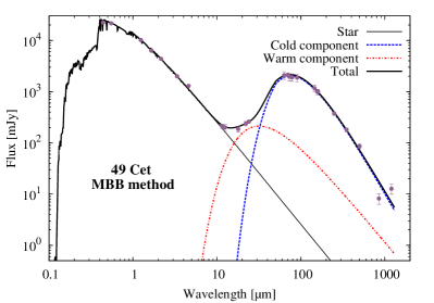
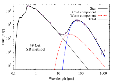
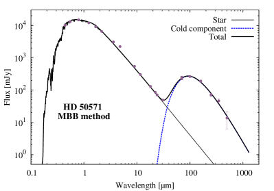
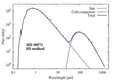
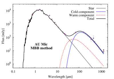
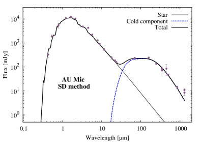
Figure 1.— The SEDs for 49 Cet (top), HD 50571 (middle), and AU Mic (bottom) fitted by the MBB method (left) and the SD method (right). Symbols with error bars are measured fluxes and their uncertainties. Lines are explained in the legend.

A detailed study of the incidence and properties of the warm component is deferred to a subsequent paper. Here we concentrate on the properties of the main, cold component and thus use the knowledge of the warm component to exclude it from the SED, as described above. The disk radii and the fitting results for the cold component obtained both with the MBB and SD methods are listed in Tables 4–5 and plotted in Figures 2–5. These are discussed in the following subsections.

Figure 2.— Disk radii versus stellar luminosities. The straight line is the best linear fit to the log-log data, equivalent to a power law fit of the form $R_{\mathrm{cold}}=a(L/L_{\odot})^{b}$. The best-fit parameters $a$ and $b$ together with the Pearson’s $r$ and Spearman’s $r_{s}$ are indicated in the panel.

4.2. Disk radii

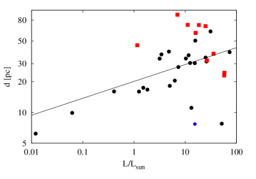
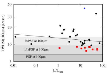
Figure 3.— Distance to targets (left) and the observed long-axis FWHM at $100\,\hbox{\textmu{}m}$ (right) as a function of stellar luminosity. Tilted straight lines are log-log best fits through the symbols. For Fomalhaut (blue diamond), the FWHM at $70\,\hbox{\textmu{}m}$ instead of $100\,\hbox{\textmu{}m}$ is shown in the right panel. Grey-shaded areas correspond to 1.0, 1.4, and 2.0 times the beam size, showing how well the disks have been resolved. Red squares are marginally resolved systems, i.e. those with $\text{FWHM}<1.4\text{PSF}$.

The cold disk radii are plotted in Figure 2. They reveal a huge scatter, from $\approx 40\,\hbox{AU}$ to $\approx 290\,\hbox{AU}$. At a first glance, the figure suggests a weak positive correlation with the stellar luminosity. However, the Pearson correlation coefficient between $\log R_{\mathrm{cold}}$ and $\log L$ is only $r=+0.38$. The Spearman rank correlation coefficient (that does not require linearity and treats possible outliers better than Pearson does) is as small as $r_{s}=0.02$. To interpret these coefficients, we can calculate a two-tailed probability that the correlation is absent. The correlation is treated as significant if this probability is less than 1%; for a sample of 34 stars, this requires $r$ or $r_{s}$ larger than 0.43. Judging by $r$ and especially by $r_{s}$, the correlation between $\log R_{\mathrm{cold}}$ and $\log L$ is unlikely. Also, the best-fit trend line $R_{\mathrm{cold}}=a(L/L_{\odot})^{b}$ has $a=123\pm 15\,\hbox{AU}$ and $b=0.04\pm 0.04$, so that the slope $b$ is statistically indistinguishable from zero. Furthermore, the results strongly depend on a few individual stars with radii far from the trend line. For example, excluding the two M-stars (which are the two points in the left bottom corner of Figure 2) would change the best-fit coefficients to $a=152\pm 20\,\hbox{AU}$ and $b=0.03\pm 0.05$.

Table 4Fitting Results for the MBB Method

HD	$r_{\text{cold}}$	$s_{\text{blow}}$	$T_{\text{BB}}$	$\lambda_{\text{0}}/(2\pi)$	$\beta$	$T_{\text{d}}$	$T_{\text{d}}/T_{\text{BB}}$	$\chi^{2}_{\text{red}}$
GJ 581	38	-	15	0.06 $\pm$ 0.44	0.74 $\pm$ 0.19	35 $\pm$ 3	2.31 $\pm$ 0.17	1.01
197481	38	-	22	0.02 $\pm$ 0.19	0.37 $\pm$ 0.08	38 $\pm$ 1	1.74 $\pm$ 0.05	2.63
23484	91	-	24	0.13 $\pm$ 0.42	0.37 $\pm$ 0.11	36 $\pm$ 3	1.53 $\pm$ 0.13	0.86
104860	105	0.39	28	9.24 $\pm$ 0.25	0.88 $\pm$ 0.07	33 $\pm$ 3	1.18 $\pm$ 0.11	3.22
207129	148	0.41	24	0.03 $\pm$ 0.70	0.53 $\pm$ 0.15	46 $\pm$ 3	1.90 $\pm$ 0.12	4.35
10647	117	0.47	28	0.13 $\pm$ 0.22	0.44 $\pm$ 0.10	47 $\pm$ 4	1.68 $\pm$ 0.14	5.02
48682	142	0.54	28	0.11 $\pm$ 0.44	0.52 $\pm$ 0.11	50 $\pm$ 3	1.78 $\pm$ 0.11	9.36
50571	138	0.81	31	5.67 $\pm$ 0.39	0.95 $\pm$ 0.10	40 $\pm$ 3	1.27 $\pm$ 0.10	1.69
170773	207	0.86	26	5.96 $\pm$ 0.56	1.08 $\pm$ 0.08	35 $\pm$ 1	1.34 $\pm$ 0.04	0.55
218396	293	1.11	24	2.64 $\pm$ 0.26	0.94 $\pm$ 0.08	37 $\pm$ 1	1.52 $\pm$ 0.04	7.15
109085	145	1.14	35	9.11 $\pm$ 0.23	0.26 $\pm$ 0.10	36 $\pm$ 1	1.03 $\pm$ 0.03	3.05
27290	134	1.35	38	3.76 $\pm$ 0.30	0.64 $\pm$ 0.10	47 $\pm$ 2	1.23 $\pm$ 0.05	11.18
95086	230	1.47	30	0.02 $\pm$ 0.30	0.45 $\pm$ 0.08	52 $\pm$ 2	1.73 $\pm$ 0.07	1.87
195627	175	1.51	34	5.56 $\pm$ 0.79	0.97 $\pm$ 0.10	43 $\pm$ 2	1.26 $\pm$ 0.06	2.14
20320	157	1.94	45	2.31 $\pm$ 0.75	0.55 $\pm$ 0.08	56 $\pm$ 2	1.24 $\pm$ 0.04	0.96
21997	150	2.06	42	5.73 $\pm$ 0.53	0.82 $\pm$ 0.08	49 $\pm$ 1	1.17 $\pm$ 0.02	0.80
110411	111	2.13	50	6.04 $\pm$ 0.38	1.22 $\pm$ 0.08	60 $\pm$ 3	1.19 $\pm$ 0.06	6.10
142091	131	2.24	45	0.05 $\pm$ 0.40	0.32 $\pm$ 0.09	63 $\pm$ 4	1.41 $\pm$ 0.09	8.47
102647	48	2.33	78	4.62 $\pm$ 0.74	1.04 $\pm$ 0.10	87 $\pm$ 1	1.12 $\pm$ 0.01	16.07
125162	112	2.61	56	5.33 $\pm$ 0.44	0.69 $\pm$ 0.08	63 $\pm$ 1	1.12 $\pm$ 0.02	4.09
216956	123	2.62	50	16.40  $\pm$ 0.18	0.85 $\pm$ 0.09	51 $\pm$ 2	1.01 $\pm$ 0.04	4.39
17848	222	2.65	37	5.05 $\pm$ 0.35	0.80 $\pm$ 0.08	45 $\pm$ 4	1.21 $\pm$ 0.11	3.66
9672	172	2.68	43	8.01 $\pm$ 0.47	0.97 $\pm$ 0.10	49 $\pm$ 2	1.16 $\pm$ 0.05	0.55
71722	111	2.99	52	3.03 $\pm$ 0.35	0.63 $\pm$ 0.07	64 $\pm$ 1	1.23 $\pm$ 0.02	8.63
182681	184	3.72	46	1.27 $\pm$ 0.35	0.74 $\pm$ 0.09	68 $\pm$ 1	1.49 $\pm$ 0.02	6.55
14055	165	3.73	51	19.73  $\pm$ 1.28	1.14 $\pm$ 0.09	51 $\pm$ 1	1.01 $\pm$ 0.02	3.02
161868	143	3.84	53	3.15 $\pm$ 0.33	0.69 $\pm$ 0.08	65 $\pm$ 1	1.22 $\pm$ 0.02	4.34
188228	106	3.90	62	0.73 $\pm$ 0.98	0.36 $\pm$ 0.12	77 $\pm$ 6	1.25 $\pm$ 0.10	1.39
10939	180	4.40	49	20.80  $\pm$ 0.48	1.22 $\pm$ 0.08	50 $\pm$ 1	1.03 $\pm$ 0.02	3.08
71155	88	4.85	72	8.65 $\pm$ 0.39	2.22 $\pm$ 0.10	79 $\pm$ 15	1.08 $\pm$ 0.21	2.17
172167	115	6.38	60	23.22  $\pm$ 1.25	1.35 $\pm$ 0.09	70 $\pm$ 3	1.18 $\pm$ 0.05	7.50
139006	61	6.90	98	11.89  $\pm$ 1.03	1.80 $\pm$ 0.10	101  $\pm$ 3	1.03 $\pm$ 0.03	1.94
95418	61	6.95	98	11.54  $\pm$ 0.93	1.37 $\pm$ 0.12	100  $\pm$ 4	1.02 $\pm$ 0.04	9.48
13161	143	8.28	69	22.60  $\pm$ 0.43	1.33 $\pm$ 0.11	68 $\pm$ 1	0.99 $\pm$ 0.01	2.56

Notes:
The disk radii are in AU, the temperatures in K and $\lambda_{\text{0}}/(2\pi)$, $s_{\text{blow}}$ in  µm.

The conclusion that $R_{\mathrm{cold}}$ and $L$ appear uncorrelated is not necessarily in contradiction with a possible weak trend of disk radius getting larger towards more luminous stars reported by Eiroa et al. (2013). The reason is that Eiroa et al. consider the blackbody radius $R_{\mathrm{BB}}$ rather than the true disk radius $R_{\mathrm{cold}}$. Below we will see that the ratio of the two, $\Gamma=R_{\mathrm{cold}}/R_{\mathrm{BB}}$, decreases with $L$, which may compensate an increase in $R_{\mathrm{BB}}$ towards higher $L$, leading to an $R_{\mathrm{cold}}$ uncorrelated with the stellar luminosity.

The above analysis should be treated with caution. One caveat is related to luminous, F- and especially A-stars. The more luminous the stars, the more distant they are on the average. Therefore, their disks often have a smaller angular size, and thus are less well resolved, as illustrated in Figure 3. It shows, for example, that all disks around stars with $L>10L_{\odot}$, except for Fomalhaut and Vega, are resolved in less than two beams. This may explain why the scatter in $R_{\mathrm{cold}}$ is larger for more luminous stars.

Another caveat is that our narrow-disk (single-radius) approximation may be rather poor for some disks where the dust distribution is strongly extended. The finite disk widths are particularly apparent in the scattered light images that are most sensitive to the small grains. For a small sample of large, bright disks, Krist et al. (2012) find the disk widths at half-maximum brightness to range from 20% to 60% of the belt radius. Also, multi-wavelength studies of some of the individual disks, especially of A-stars such as Vega (Su et al. 2006) and HR 8799 (Matthews et al. 2014a) reveal huge halos probably composed of small dust grains in weakly bound orbits (Matthews et al. 2014b). For instance, the huge ($290\,\hbox{AU}$) radius derived from the HR 8799 PACS image may not necessarily measure the “peak” radius of the disk (i.e. the radius of the dust-producing planetesimal belt).

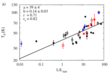
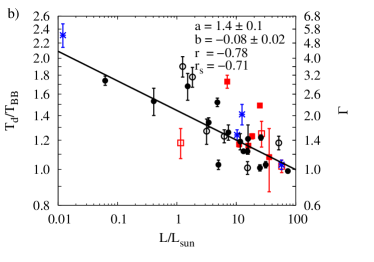
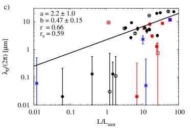
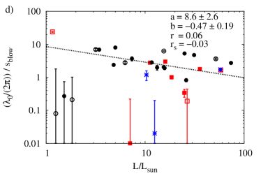
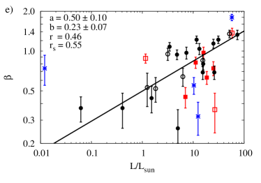
Figure 4.— Disk parameters obtained with the MBB method, plotted as functions of stellar luminosity: (a) dust temperature, (b) the ratio of the dust temperature to the blackbody temperature and the ratio $\Gamma$ of the true disk radius to its blackbody radius, (c) the characteristic size $\lambda_{0}/(2\pi)$, (d) the ratio of $\lambda_{0}/(2\pi)$ to the blowout size $s_{\mathrm{blow}}$ for stars with $L>L_{\odot}$, and (e) the opacity index $\beta$. Open and filled symbols stand for one- and two-component disks, respectively. Circles represent well-resolved disks, squares indicate marginally resolved ones. The blue asterisks are the objects with no (sub)-mm detections. Lines are linear fits to the log-log data. The quantities $a$, $b$, $r$, and $r_{s}$ are as in Figure 2. The trend lines are solid if a correlation is formally significant (both $r$ and $r_{s}$ are greater than 0.43) and dashed otherwise.

4.3. Dust temperatures and sizes assuming MBB

The temperature as a function of the luminosity of the primary stars is plotted in Figure 4a. It shows that the dust temperature rises from 30–50 K for late- and solar-type stars to $60$–$100\,\hbox{K}$ for the most luminous A-stars. With the Pearson’s $r=0.71$ and the Spearman’s $r_{s}=0.82$, the trend is very significant. This is in a good agreement with other Herschel-based studies, most notably Booth et al. (2013) who find temperatures in the $70$–$120\,\hbox{K}$ range for their sample of A-stars. Our results are also roughly consistent with Spitzer results by Morales et al. (2011), although a trend of temperatures getting warmer towards A-stars was weaker there. They find median values for their samples of G- and A-stars to be close to each other — $59\,\hbox{K}$ and $62\,\hbox{K}$, respectively. We can also compare the temperatures with the [24]-[70] color temperatures of 44 A-star disks derived by Su et al. (2006) (see their Figure 7). For a subsample of eight A-stars only detected at $70\,\hbox{\textmu{}m}$ but not at $24\,\hbox{\textmu{}m}$, the upper limits on the temperature vary between $60\,\hbox{K}$ and $120\,\hbox{K}$, with the median value of $79\,\hbox{K}$. Most recently, Ballering et al. (2013) studied the circumstellar environment of more than 500 main-sequence stars using Spitzer IRS/MIPS data. Considering the SEDs of 174 debris disks, they found a correlation between the temperature of cold debris component and stellar temperature. Our Figure 4a is in excellent agreement with their Figure 5.

Figure 4b presents the ratio $T_{\mathrm{dust}}/T_{\mathrm{BB}}$, where $T_{\mathrm{BB}}\propto L^{1/4}R_{\mathrm{cold}}^{-1/2}$ is the blackbody temperature at a distance $R_{\mathrm{cold}}$ from the star. If the variation in $T_{\mathrm{dust}}$ seen in Figure 4a were caused solely by different luminosities of the central stars and differences in the radii between the individual disks, the ratio $T_{\mathrm{dust}}/T_{\mathrm{BB}}$ would be nearly constant for all the systems. Instead, we see a clear trend of $T_{\mathrm{dust}}/T_{\mathrm{BB}}$ decreasing with the increasing stellar luminosity ($r=-0.78$, $r_{s}=-0.71$), in a good agreement with Booth et al. (2013). An equivalent quantity to $T_{\mathrm{dust}}/T_{\mathrm{BB}}$ is $\Gamma=(T_{\mathrm{dust}}/T_{\mathrm{BB}})^{2}$, which is the ratio of the true disk radius to the radius it would have if its material were emitting as blackbody (Booth et al. 2013). To facilitate comparisons with the results obtained by other authors, we plot $\Gamma$ in the second axis of Figure 4b. The trend of $T_{\mathrm{dust}}/T_{\mathrm{BB}}$ or $\Gamma$ decreasing with $L$ must be indicative of dust grains getting larger in disks of earlier-type stars, because bigger grains are colder.

Table 5Fitting Results for the SD Method

HD	$r_{\text{cold}}$	$s_{\text{blow}}$	$T_{\text{BB}}$	$s_{\text{min}}$	$q$	$T_{\text{d}}$	$T_{\text{d}}/T_{\text{BB}}$	$\chi^{2}_{\text{red}}$
GJ 581	38	-	15	1.50 $\pm$ 2.32	3.37 $\pm$ 0.60	24 $\pm$ 11	1.59 $\pm$ 0.74	0.78
197481	38	-	22	0.21 $\pm$ 2.27	3.33 $\pm$ 0.43	42 $\pm$ 12	1.93 $\pm$ 0.55	5.28
23484	91	-	24	1.46 $\pm$ 2.45	3.41 $\pm$ 0.45	37 $\pm$ 10	1.56 $\pm$ 0.42	1.56
104860	105	0.39	28	6.96 $\pm$ 2.41	3.83 $\pm$ 0.40	44 $\pm$ 10	1.58 $\pm$ 0.36	2.99
207129	148	0.41	24	4.93 $\pm$ 1.67	4.23 $\pm$ 0.46	56 $\pm$ 16	2.33 $\pm$ 0.67	6.19
10647	117	0.47	28	3.92 $\pm$ 2.21	3.87 $\pm$ 0.37	56 $\pm$ 11	2.00 $\pm$ 0.39	5.33
48682	142	0.54	27	1.83 $\pm$ 2.73	3.70 $\pm$ 0.60	65 $\pm$ 11	2.42 $\pm$ 0.41	4.62
50571	138	0.81	31	5.36 $\pm$ 2.75	4.01 $\pm$ 0.49	56 $\pm$ 13	1.80 $\pm$ 0.41	1.85
170773	207	0.86	26	5.04 $\pm$ 2.83	4.02 $\pm$ 0.46	53 $\pm$ 7	1.99 $\pm$ 0.26	3.37
218396	293	1.11	24	4.84 $\pm$ 2.72	4.01 $\pm$ 0.55	51 $\pm$ 11	2.11 $\pm$ 0.46	6.42
109085	145	1.14	35	7.46 $\pm$ 1.81	2.85 $\pm$ 0.40	35 $\pm$ 17	1.01 $\pm$ 0.49	1.80
27290	134	1.35	38	5.02 $\pm$ 2.11	3.85 $\pm$ 0.31	61 $\pm$ 18	1.60 $\pm$ 0.48	37.36
95086	230	1.47	30	2.96 $\pm$ 3.54	3.83 $\pm$ 0.54	61 $\pm$ 19	2.03 $\pm$ 0.64	1.30
195627	175	1.51	34	4.83 $\pm$ 1.90	4.00 $\pm$ 0.41	61 $\pm$ 7	1.78 $\pm$ 0.21	2.24
20320	157	1.94	45	5.38 $\pm$ 2.56	3.90 $\pm$ 0.59	68 $\pm$ 7	1.50 $\pm$ 0.15	0.52
21997	150	2.06	42	4.46 $\pm$ 1.88	3.88 $\pm$ 0.33	65 $\pm$ 16	1.57 $\pm$ 0.39	1.28
110411	111	2.13	50	3.42 $\pm$ 1.91	4.10 $\pm$ 0.44	87 $\pm$ 21	1.73 $\pm$ 0.42	9.21
142091	131	2.24	45	2.42 $\pm$ 2.85	3.64 $\pm$ 0.43	73 $\pm$ 15	1.61 $\pm$ 0.33	7.61
102647	48	2.33	78	8.84 $\pm$ 2.14	4.24 $\pm$ 0.44	72 $\pm$ 11	0.92 $\pm$ 0.14	1.79
125162	112	2.61	56	3.94 $\pm$ 2.11	3.75 $\pm$ 0.52	78 $\pm$ 8	1.39 $\pm$ 0.14	3.95
216956	123	2.62	50	3.88 $\pm$ 2.64	3.44 $\pm$ 0.39	63 $\pm$ 12	1.25 $\pm$ 0.24	3.51
17848	222	2.65	37	4.69 $\pm$ 2.11	3.88 $\pm$ 0.38	62 $\pm$ 6	1.66 $\pm$ 0.16	3.85
9672	172	2.68	43	3.98 $\pm$ 2.02	3.85 $\pm$ 0.38	70 $\pm$ 16	1.64 $\pm$ 0.38	1.08
71722	111	2.99	52	5.11 $\pm$ 1.63	3.94 $\pm$ 0.61	75 $\pm$ 21	1.44 $\pm$ 0.40	9.16
182681	184	3.72	46	2.47 $\pm$ 1.74	3.95 $\pm$ 0.44	90 $\pm$ 19	1.97 $\pm$ 0.42	2.32
14055	165	3.73	51	6.70 $\pm$ 3.18	3.69 $\pm$ 0.40	63 $\pm$ 19	1.24 $\pm$ 0.37	3.07
161868	143	3.84	53	4.81 $\pm$ 2.41	3.72 $\pm$ 0.36	72 $\pm$ 7	1.35 $\pm$ 0.13	9.61
188228	106	3.90	62	1.81 $\pm$ 3.71	3.34 $\pm$ 0.33	79 $\pm$ 24	1.28 $\pm$ 0.39	1.50
10939	180	4.40	49	8.81 $\pm$ 1.90	3.78 $\pm$ 0.38	59 $\pm$ 5	1.20 $\pm$ 0.10	4.00
71155	88	4.85	72	5.14 $\pm$ 2.12	5.80 $\pm$ 0.41	104 $\pm$ 38	1.44 $\pm$ 0.52	2.94
172167	115	6.38	60	9.05 $\pm$ 1.91	3.67 $\pm$ 0.34	68 $\pm$ 2	1.14 $\pm$ 0.03	9.87
139006	61	6.90	98	6.74 $\pm$ 2.50	5.29 $\pm$ 0.41	97 $\pm$ 44	0.99 $\pm$ 0.45	2.35
95418	61	6.95	98	5.18 $\pm$ 2.12	4.43 $\pm$ 0.33	110 $\pm$ 43	1.12 $\pm$ 0.44	9.50
13161	143	8.28	71	15.09  $\pm$ 2.49	4.47 $\pm$ 0.37	59 $\pm$ 6	0.82 $\pm$ 0.08	3.46

Notes:
The disk radii are in AU, the temperatures in K and $s_{\text{blow}}$ and $s_{\mathrm{min}}$ in  µm.

To check this, in Figure 4c we plot the quantity $\lambda_{0}/(2\pi)$, which is a proxy for the typical grain sizes in the MBB method. Indeed, there is a strong ($r=0.66$, $r_{s}=0.59$) trend of the typical size increasing with the stellar luminosity. That size rises from $\lesssim 1\,\hbox{\textmu{}m}$ for GKM-type stars to a few  µm or even more for A-type stars.

We expect that the reason for the dust sizes to increase towards more luminous stars is that so does the radiation pressure blowout limit. To verify this, we calculate it as (see, e.g., Burns et al. 1979):

$${\frac{s_{\mathrm{blow}}}{1\,\hbox{\textmu{}m}}}=0.35Q_{\mathrm{pr}}\left(\frac{3.3\,\hbox{g}\,\hbox{cm}^{-3}}{\rho}\right)\left(\frac{L/L_{\odot}}{M/M_{\odot}}\right),$$ (7)

where $\rho$ is the grain’s bulk density, $L$ and $M$ are stellar luminosity and mass, and $Q_{\mathrm{pr}}$ is the radiation pressure efficiency. We adopted $\rho=3.3\,\hbox{g}\,\hbox{cm}^{-3}$ and took $L$ and $M$ from Table 2. Next, we assumed $Q_{\mathrm{pr}}=1$. As long as $L\geq L_{\odot}$, the error introduced by this assertion is much smaller than the accuracy of the $\lambda_{0}/(2\pi)$ determination. For instance, the astrosilicate particles with $s=s_{\mathrm{blow}}$ around a $1L_{\odot}$ and a $10L_{\odot}$ star would have $Q_{\mathrm{pr}}=1.4$ and $Q_{\mathrm{pr}}=1.1$, respectively. If $L<L_{\odot}$, the assumption $Q_{\mathrm{pr}}=1$ is no longer valid. One has to consider $Q_{\mathrm{pr}}$ as a function of the grain size and treat the formula (7) as an equation for $s_{\mathrm{blow}}$. For low-luminosity stars, this equation will not have a solution, meaning that radiation pressure is too weak for the blowout limit to exist. For this reason, we only calculated $s_{\mathrm{blow}}$ for stars with $L\geq L_{\odot}$.

The result is shown in Figure 4d. We find that $\lambda_{0}/(2\pi)$ for nearly all the stars lies in the range from $(1...10)s_{\text{blow}}$, regardless of the stellar luminosity. Judging by the trend line, there might be a subtle trend of the $\lambda_{0}/(2\pi)$ to $s_{\text{blow}}$ ratio decreasing towards earlier spectral classes (the slope $-0.47$). However, the correlation coefficients are as small as $r=+0.06$ and $r_{s}=-0.03$. The Spearman probability that the ratio of $\lambda_{0}/(2\pi)$ to $s_{\text{blow}}$ is constant is 87%.

Finally, Figure 4e depicts the MBB index $\beta$. As expected, it lies between 0 and 2, with the majority of disks best fitted with $\beta$ between zero and unity. This is consistent with previous results, based on sub-mm observations of debris disks (e.g., Williams & Andrews 2006; Nilsson et al. 2010). There might be a slight trend of $\beta$ increasing with the stellar luminosity. However, with $r=0.46$ and $r=0.55$, the trend is only of moderate significance. If it is real, it may be a consequence of the fact that $\beta$ is not completely independent of $\lambda_{0}$ (see Appendix B).

4.4. Dust temperatures and sizes assuming SD

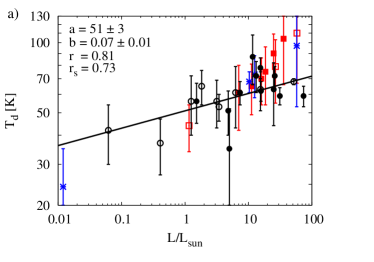
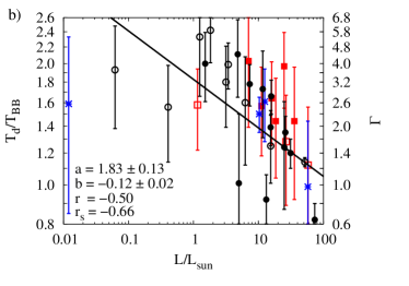
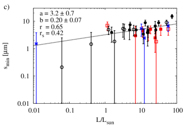
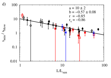
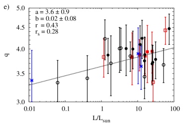
Figure 5.— Disk parameters obtained with the SD method, plotted as functions of stellar luminosity: (a) dust temperature, (b) the ratio of the dust temperature to the blackbody temperature and the ratio of the true disk radius to its blackbody radius, (c) minimum size $s_{\mathrm{min}}$, (d) the ratio of $s_{\mathrm{min}}$ and $s_{\mathrm{blow}}$ for stars with $L>L_{\odot}$, and (e) the size distribution index $q$. The meaning of symbols and fitting lines is the same as in Figure 4.

We now present the results obtained with the second method of the SED fitting, which assumed a size distribution of particles and their particular emitting properties (here: astrosilicate). Figure 5 is organized in a similar way as Figure 4, with the only difference that we now plot $s_{\mathrm{min}}$ instead of $\lambda_{0}/(2\pi)$ and $q$ instead of $\beta$.

The temperature plots, i.e. $T_{\mathrm{dust}}$ and $T_{\mathrm{dust}}/T_{\mathrm{BB}}$, readily show some quantitative differences to the MBB method. These are already visible at the level of individual stars. For instance, one of the two M-stars in our sample, GJ 581, reveals a smaller $s_{\mathrm{min}}$ than earlier-type stars, consistent with the general trend. However, the dust temperature ($T_{\mathrm{dust}}$ in Figure 5a, $T_{\mathrm{dust}}/T_{\mathrm{BB}}$ in Figure 5b) is much lower that one might expect. This might seem strange, as smaller grains are usually hotter, not colder, than larger ones. However, this can be easily explained with absorption properties of the astrosilicate, whose absorption efficiency in the visible (i.e. where the stellar light is absorbed) drops drastically at small grain sizes. As a result, small particles become colder again (Krivov et al. 2008). For M-stars such as GJ 581, this happens for grains smaller than a few microns.

Notwithstanding some individual cases, the temperatures derived with the SD method show the same qualitative trends as those obtained with the MBB. The dust temperature grows with luminosity (Figure 5a), the ratio of the dust temperature to the blackbody temperature decreases (Figure 5b), and the minimum grain size gets larger towards more luminous stars (Figure 5c). Judging by the Pearson’s correlation coefficient as indicated in the panels, all of these trends are significant. Spearman’s ranking suggests the same, except that the $s_{\mathrm{min}}$–$L$ correlation has $r=0.42$ and is only moderately significant at a 1% level. However, quantitative differences from the MBB results are not to be overlooked. The increase of temperature towards larger $L/L_{\odot}$ is now weaker, the decrease of $T_{\mathrm{dust}}/T_{\mathrm{BB}}$ stronger, and $s_{\mathrm{min}}$ (Figure 5c) increases with $L/L_{\odot}$ more gently than $\lambda_{0}/(2\pi)$ does. As a consequence, the inferred sizes are more consistent with $s_{\mathrm{min}}/s_{\mathrm{blow}}$ decreasing towards more luminous stars from $\sim 10$ for solar-type stars to nearly unity for A-stars (Figure 5d). Interestingly, this trend is formally the strongest of all correlations found in our paper ($r=-0.85$, $r_{s}=-0.86$, significance $<10^{-8})$! This needs to be explained, and we will return to this in Sect. 5.

Finally, the slope $q$ lies between 3.3 and 4.5 for nearly all the stars (Figure 5e), being close to the “canonical” value 3.5 (Dohnanyi 1969). Like $\beta$ in the MBB method, it seems to reveal a trend of $q$ increasing with the stellar luminosity, with a marginal significance ($r=0.43$, $r_{s}=0.28$). However, the apparent trend is primarily caused by three individual stars of subsolar luminosity. Excluding these would lead to $r=0.28$, suggesting that the trend may not be real. Also, similar to the MBB method, this might trace back to the shape of the $\chi^{2}$-isolines discussed in Appendix B.

4.5. MBB versus SD

Why are the results of the MBB and SD methods somewhat different, and which of these are more trustworthy? The main reason for the differences is that both methods yield SEDs of different shape, and that shape responds differently to the variation of fitting parameters. An SED generated with the MBB method consists of a Planck curve at $\lambda<\lambda_{0}$ and a steeper Rayleigh-Jeans tail at $\lambda>\lambda_{0}$, separated by an artificial knee at $\lambda_{0}$. Thus the entire modeled SED can only be narrower than a Planck curve. In contrast, the SD method assumes a continuous distribution of particle sizes (and thus temperatures) and is able to yield smooth SEDs that are broader than a single-temperature blackbody curve (Figure 1, bottom panels). Furthermore, with this method we are at liberty to vary the dust composition and structure by varying $Q_{\mathrm{abs}}(\lambda,s)$, which makes the fitting even more flexible. Altogether, we expect the SD method to be superior to the MBB one. Nevertheless, we deem it reasonable to present results obtained with both techniques. This is because the MBB approximation is simple, transparent, and may be more appropriate for stars with relatively sparse SEDs. Next, the MBB results can be directly compared to those derived by other authors, many of which employ this technique. Finally, a comparison between the MBB and SD results allows us to better judge how significant our findings are. If one or another trend is evident with both methods, this can be treated as an additional argument that the trend may be real.

4.6. Origin of scatter

Most of the plots presented above reveal an appreciable scatter amongst the data points. What is the origin of this scatter? Some of it may reflect real differences between individual systems of any spectral class, but much of it likely comes from uncertainties of numerous parameters and measurements themselves. These include not only a random, but also a systematic component. This makes it difficult to find out, for instance, whether a somewhat larger scatter at higher luminosities reflects a higher degree of dissimilarity of debris disks around more luminous stars or is caused by larger uncertainties associated with such stars.

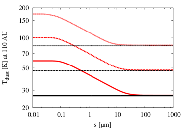
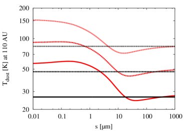
Figure 6.— Equilibrium temperature of dust grains (red lines) and blackbody temperature (black) against grain size. Top: MBB dust grains, bottom: astrosilicate particles. Solid lines: $L_{*}=L_{\odot}$, dashed: $L_{*}=10L_{\odot}$, dotted: $L_{*}=100L_{\odot}$.

To illustrate this, let us consider A-stars. Modeling of their disks uncovers three serious problems. The first one is a poorer accuracy of disk radius determination for A-stars, as discussed in Sect. 4.1. The second problem is that in the case of A-stars the dust temperature turns out to be particularly sensitive to the set of photometry points used for the fitting (even including or excluding one single point can matter), and to the fitting method (MBB versus SD). This is because the IR excesses in the SEDs of A-stars peak at shorter wavelengths than those of later-type stars. Often the SED maximum lies between $\sim 30\,\hbox{\textmu{}m}$ (where the IRS spectra end) and $60$–$70\,\hbox{\textmu{}m}$ (where the MIPS and PACS data start), i.e. at wavelengths that have never been probed by any IR instruments. The third problem is that $s_{\mathrm{min}}$ is also very sensitive to the dust temperature, especially for A-stars. This can be understood by looking at Figure 6, where we plotted the temperature of grains calculated with two methods. In one case (upper panel), we used the “MBB grains”, whose absorption efficiency is given by Eq. (2). In another case (lower panel), we assumed the absorption efficiency of astrosilicate. For the explanations of the resulting temperature behavior the reader is referred to Krivov et al. (2008), where also $Q_{\textrm{abs}}(\lambda)$ curves for different-sized grains are plotted. It is seen that for luminous stars, the grains with radii between several microns and several tens of microns have temperatures close to $T_{\mathrm{BB}}$. For astrosilicate grains, $T_{\mathrm{dust}}$ may even be below $T_{\mathrm{BB}}$. Thus a small change in $T_{\mathrm{dust}}$ for those stars would imply a large change in $s_{\mathrm{min}}$. Therefore, for A-stars we are facing three challenges at the same time: it is difficult to accurately measure the disk radii from the images, it is difficult to derive $T_{\mathrm{dust}}$ from the Herschel photometry, and it is difficult then to derive $s_{\mathrm{min}}$ from $T_{\mathrm{dust}}$. This makes the results of disks of A-stars intrinsically more uncertain than those for later-type stars.

5. Discussion

5.1. Disk radii and dust sizes

One thing that we have learned is that the radii of the resolved debris disks appear uncorrelated with the luminosity of their host stars, and that there is a large scatter of radii at any given luminosity. This confirms that the temperature-dependent processes such as ice lines do not play the dominant role in setting the debris disk dimensions (Ballering et al. 2013). However, a conclusion that the planetesimal formation is not directly related to such processes would be premature. This is because the location of debris disks depends not only on the location of zones where planetesimals preferentially form, but also on the subsequent complex dynamical and collisional evolution of these planetesimals. It is thus possible that planetesimal formation mechanisms are temperature-driven, for instance are largely related to location of ice lines (e.g. Dodson-Robinson et al. 2009; Ros & Johansen 2013), but the emerging debris disks are shaped by processes that are temperature-independent. The latter may include, for instance, shaping of planetesimal populations by planets, stirring by various mechanisms, and long-term collisional depletion.

Next, we have confirmed that the dust temperature in Kuiper belt-like disks is higher around more luminous stars, as found previously (e.g. Ballering et al. 2013; Booth et al. 2013; Eiroa et al. 2013; Chen et al. 2014). However, the temperature rise with the stellar luminosity is gentler than the one we could expect if the sizes of dust grains were the same of all the stars, as first pointed out by Booth et al. (2013). Instead, the grains in disks of more luminous stars must be colder, and thus bigger. We attribute this to direct radiation pressure that swiftly eliminates all grains with sizes $s<s_{\mathrm{blow}}$, where the blowout limit $s_{\mathrm{blow}}$ is larger at higher stellar luminosities. We have shown that the ratio of the dominant grain size to the blowout size lies between roughly one and ten at all luminosities. This confirms theoretical predictions and provides direct evidence that radiation pressure does play the leading role in setting the size distribution of debris disks.

5.2. Dust properties

In Section 4.4, we noted that the SD method uncovered a significant trend of $s_{\mathrm{min}}/s_{\mathrm{blow}}$ decreasing with $L$. A similar trend, albeit at a low significance level, was also seen in the MBB results. This correlation certainly needs to be verified in the future studies over larger samples. However, should this trend be real, it requires explanation.

One possibility is to attribute it to the dust properties. Our modeling assumed compact, spherical astrosilicate particles. However, the reality is expected to be more complex: e.g. different mixtures of ices, silicates, and organics, and different packing factors, around stars of different spectral types. Indeed, detailed models of individual debris disks often favor more realistic dust compositions (e.g. Lebreton et al. 2012; Donaldson et al. 2013). This is not any surprise, since the material in debris disks should inherit such a complex chemistry and morphology from the preceding, protoplanetary phase (Dutrey et al. 2014). Another piece of evidence for rich composition of debris material comes from the analysis of the oldest debris disk systems, namely from the spectra of debris-polluted white dwarfs (Zuckerman et al. 2003; Gänsicke et al. 2006; Farihi et al. 2009).

Changing the grain properties (chemical composition and porosity and thus $Q_{\textrm{abs}}$, $Q_{\textrm{pr}}$, and $\rho$) may change the results considerably. For instance, if dust grains are icy, the blowout size changes compared to that of pure silicate in a non-trivial way (see, e.g., Figure 2 in Reidemeister et al. 2011). For G-type stars, $s_{\mathrm{blow}}$ remains nearly unchanged, but for A-stars, it decreases considerably. However, the icy grains of a given size at a given distance from the star are colder than silicate ones, and so, we may expect that $s_{\mathrm{min}}$ derived from the SED fitting will be smaller. This effect could make the ratio $s_{\mathrm{min}}/s_{\mathrm{blow}}$ more uniform than Figure 5d suggests. However, further modeling, which is outside the scope of this paper, is required to find out how exactly the ratio $s_{\mathrm{min}}/s_{\mathrm{blow}}$ will be affected.

The grains can also be moderately or even very porous. This, too, would change $s_{\mathrm{blow}}$ (see, e.g., Figures 7–8 in Kirchschlager & Wolf 2013). Porosity moderately increases $s_{\mathrm{blow}}$ for G-stars. For A-stars, $s_{\mathrm{blow}}$ will strongly increase compared to compact silicate grains. However, $s_{\mathrm{min}}$ will be affected as well, since porous grains have lower absorption in the visible (see, e.g., Figure 3 in Kirchschlager & Wolf 2013) and thus a lower temperature than the compact grains. Modeling is needed here, too, to describe quantitatively the changes in the ratio $s_{\mathrm{min}}/s_{\mathrm{blow}}$ caused by porosity.

5.3. Stirring level

Besides dust properties, the trends of dust sizes around stars of different luminosities can also be affected by the following effect. Assume that, for whatever reasons, the disks around early-type stars are more strongly stirred than those of later-type ones. One can indeed expect this, as more luminous stars are more massive, and may have had more massive protoplanetary disks (e.g. Williams & Cieza 2011), which may have been able to build larger stirring planetesimals (e.g. Kenyon & Bromley 2008; Kobayashi et al. 2011).

If this is true, this will modify the inferred size distribution, shifting the dominant dust size to smaller values, which are closer to $s_{\mathrm{blow}}$ (e.g. Thébault & Wu 2008; Krivov et al. 2013). This could possibly explain what is seen in Figure 5d.

What is more, the alleged higher stirring level in disks of early-type stars should also affect the radial distribution of material, by making them more extended beyond the location of their parent belts (e.g. Thébault & Wu 2008; Krivov et al. 2013). Conversely, the disks of later-type stars may tend to stretch inward from the location of the birth belts. In fact, this seems to be supported by observations. Several disks of A-stars are known to have pronounced halos and rather sharp inner edges (examples: Vega, Su et al. 2005, Müller et al. 2010; HR 8799, Su et al. 2009, Matthews et al. 2014a), whereas some disks of late-type stars have sharper outer edges and a leakage of dust into the cavities (like that of HD 107146, Ertel et al. 2011, and HD 207129, Löhne et al. 2012). In that case, the disk radii retrieved from the resolved images would be overestimated around early-type stars and/or underestimated around late-type ones. In other words, the disks of A-type stars may be smaller than we think, while those around FGKM-type stars may be larger. To compensate for this, we would need to make the grains in disks of early-type stars cooler (and thus larger), and grains in disks of later-type stars warmer (and thus smaller). Especially for the early-type stars the effect can be significant, i.e., a slight overestimation of their disk radii would lead to a strong underestimation of the grain sizes. This is because the temperature of disks of A-stars is close to the blackbody one, so that a substantial increase of the grain size is needed to decrease their temperature only slightly.

5.4. The smallest collisional fragments

All of the previous debris disk models tacitly assumed that collisions produce fragments of all sizes down to macromolecular ones, and that the minimum size $s_{\mathrm{min}}$ is set by one or another physical process that swiftly eliminates the smallest debris from the system. However, Krijt & Kama (2014) recently realized that tiny fragments below a certain size may not be even produced. This is because a fraction of the impact energy available at any collisional event, $\eta$, has to be spent to create surfaces of the collisionally produced grains. This provides a constraint on the minimum possible grain size which can be calculated as a function of stellar mass and luminosity, disk radius, the fraction $\eta$ just described, the surface tension of the disk material $\gamma$, and the typical collisional velocity in the units of the local Keplerian speed $f$ (Equation 7 in their paper). The constraint is the strongest (i.e., the minimum size is the largest) for the least luminous stars, the largest disks, and/or the disks with the lowest dynamical excitation. Regrettably, most of these parameters, especially $\eta$, $\gamma$, and $f$, are not or only poorly known. Nevertheless, we made estimates with the default values assumed by Krijt & Kama (2014) to find that the minimum fragment size set by the surface energy constraint can be on the order of $\sim 10s_{\mathrm{blow}}$ for solar-type stars, decreasing to below $s_{\mathrm{blow}}$ for the A-type ones. This is astonishingly close to our results plotted in Figure 5d, suggesting this effect as another potential explanation for the trends of grain sizes deduced in this work.

6. Conclusions

In this paper, we considered a sample of 34 selected debris disks around AFGKM-type stars, trying to find correlations between the disk parameters and stellar luminosity. Since these disks are well-resolved, we can measure the disk radii, thus breaking the degeneracy between the grain size and dust location in the SED modeling. We employ two different methods of the SED fitting: using the modified blackbody approximation in which the typical grain size is given by $\lambda_{0}/(2\pi)$, and fitting with astrosilicate particles having a size distribution, which gives the cutoff size $s_{\mathrm{min}}$. Our key findings are as follows:

Disk radii. The disk radii were found to have a large dispersion for host stars of any spectral class, but no significant trend with the stellar luminosity is seen. This finding does not necessarily speak against suggestions that formation of planetesimals (including those that are large enough to build planets by core accretion) is largely related to location of ice lines. It is still possible that planetesimal formation is driven by temperature-dependent processes, but the final dimensions of debris disks are determined by the subsequent collisional evolution of planetesimal belts or their alteration by planetary perturbers, i.e. by processes that are obviously temperature-indepenent.

Dust temperature. The dust temperature systematically increases towards earlier spectral types. However, the ratio of the dust temperature $T_{\mathrm{dust}}$ to the blackbody temperature $T_{\mathrm{BB}}$ at the disk radius decreases with the stellar luminosity.

Minimum size of dust grains. The decrease of $T_{\mathrm{dust}}/T_{\mathrm{BB}}$ is explained by an increase of the typical grain sizes towards more luminous stars. Such a trend is expected, because radiation pressure exerted on the dust grains should get stronger towards earlier spectral types, and we do confirm it with our analysis. From M- to A-stars, both $\lambda_{0}/(2\pi)$ and $s_{\mathrm{min}}$ rise roughly from $\sim 0.1\,\hbox{\textmu{}m}$ to $\sim 10\,\hbox{\textmu{}m}$. Larger grains are colder than smaller ones and have temperatures closer to $T_{\mathrm{BB}}$. For spectral classes earlier than K where radiation pressure is strong enough for the blowout limit $s_{\mathrm{blow}}$ to exist, the typical grain size is found to lie between one and ten times $s_{\mathrm{blow}}$. This agrees very well with theoretical predictions. The ratio $s_{\mathrm{min}}/s_{\mathrm{blow}}$ appears to decrease slightly towards A-stars. Should the latter be confirmed, it might indicate, for instance, that earlier-type stars have disks that are more excited dynamically and thus are more active collisionally than those of later-type stars.

Size distribution index. The spectral index of the dust opacity $\beta$ in the modified blackbody treatment is in the range of 0.3 to 2.0 for all the disks in the sample, in accord with previous determinations based on sub-mm data. The index $q$ of the size distribution varies from 3.3 to 4.6. This is roughly consistent with what is predicted by detailed models of collisional cascade.

Appendix A A. Photometry of the systems

Table 6 lists the mid-IR photometry data for all the systems in our sample. Table 7 does the same for the far-IR and sub-millimeter photometry.

Table 6Mid-IR Photometry Used in Creating the Target SEDs

Target (HD)
	Flux [mJy]
Wavelength	11.56$\mu$m	16$\mu$m	18$\mu$m	22$\mu$m	22.09$\mu$m	24$\mu$m	31$\mu$m	Note
Instrument	b	a	c	a	b	d	a
GJ 581	213 $\pm$ 19	108 $\pm$ 1	…	58.8 $\pm$ 1.0	…	…	31.4 $\pm$ 1.3	(3)
197481	543 $\pm$ 60	…	246 $\pm$ 36	183 $\pm$ 21	…	158 $\pm$ 3	…
23484	314.4 $\pm$ 5.2	172 $\pm$ 6	…	90.3 $\pm$ 8.4	90.4 $\pm$ 2.0	80.47 $\pm$ 5.09	56.6 $\pm$ 15.4	(2)
104860	81.1 $\pm$ 1.1	44.49 $\pm$ 2.93	…	24.73 $\pm$ 3.53	23.3 $\pm$ 1.1	21.54 $\pm$ 2.91	13.36 $\pm$ 3.10
207129	635 $\pm$ 8	371 $\pm$ 5	262 $\pm$ 31	197 $\pm$ 4	196 $\pm$ 5	155 $\pm$ 3	114 $\pm$ 5	(2)
10647	600.2 $\pm$ 7.7	…	315.3 $\pm$ 39.7	…	218.1 $\pm$ 4.0	184.8 $\pm$ 3.8	185.4 $\pm$ 7.3
48682	774 $\pm$ 11	425 $\pm$ 12	458 $\pm$ 17	240 $\pm$ 5	246 $\pm$ 5	193 $\pm$ 4	152 $\pm$ 4	(2)
50571	303 $\pm$ 4	152 $\pm$ 4	129 $\pm$ 12	82.7 $\pm$ 5.0	85.4 $\pm$ 1.9	70.4 $\pm$ 2.8	48.0 $\pm$ 4.0	(2)
170773	262 $\pm$ 3	136 $\pm$ 5	…	78.4 $\pm$ 5.7	76.4 $\pm$ 2.2	65.3 $\pm$ 2.6	54.6 $\pm$ 6.0	(2)
218396	258 $\pm$ 4	140 $\pm$ 2	119 $\pm$ 80	91.3 $\pm$ 2.3	94.7 $\pm$ 2.8	86.6 $\pm$ 1.7	68.0 $\pm$ 2.3	(2)
109085	1460 $\pm$ 70	…	820 $\pm$ 20	…	680 $\pm$ 40	590 $\pm$ 20	…	(4)
27290	1269.12 $\pm$ 9.35	704.8 $\pm$ 12.7	…	263.3 $\pm$ 8.9	367.76 $\pm$ 7.11	315.6 $\pm$ 3.2	…
95086	62.7 $\pm$ 3.0	…	…	46.7 $\pm$ 7.3	51.6 $\pm$ 3.3	45.6 $\pm$ 2.0	96.7 $\pm$ 10.0	(1)
195627	761 $\pm$ 10	439.6 $\pm$ 8.3	325 $\pm$ 13	248.5 $\pm$ 6.7	237 $\pm$ 5	186 $\pm$ 7	159.46 $\pm$ 4.85
20320	…	333.5 $\pm$ 6.6	263.5 $\pm$ 56.0	186.8 $\pm$ 5.0	…	162.6 $\pm$ 4.2	109.18 $\pm$ 2.94
21997	106.6 $\pm$ 5.2	…	…	…	57.2 $\pm$ 3.7	55.1 $\pm$ 2.2	92.3 $\pm$ 10.3	(1)
110411	247.4 $\pm$ 7.2	…	204.2 $\pm$ 18.3	162.8 $\pm$ 6.0	…	149.7 $\pm$ 3.9	…
142091	…	…	…	…	890.4 $\pm$ 13.1	800.1 $\pm$ 8.0	…
102647	…	2989 $\pm$ 48	…	1724 $\pm$ 30	…	1647 $\pm$ 33	…
125162	…	442 $\pm$ 5	415.7 $\pm$ 15.6	310 $\pm$ 6	…	270.8 $\pm$ 2.3	276 $\pm$ 6	(2)
216956	…	6947 $\pm$ 112	5338 $\pm$ 81.8	3940 $\pm$ 64	…	3502 $\pm$ 64	…	(4)
17848	315 $\pm$ 4	177.3 $\pm$ 3.6	105 $\pm$ 10	99.82 $\pm$ 2.75	102 $\pm$ 2	88.68 $\pm$ 2.44	68.26 $\pm$ 1.87
9672	211 $\pm$ 21	…	…	…	238 $\pm$ 24	259 $\pm$ 10	426 $\pm$ 1	(1)
71722	141 $\pm$ 2	85.67 $\pm$ 1.83	…	65.16 $\pm$ 1.81	63.4 $\pm$ 2.1	62.53 $\pm$ 1.73	76.70 $\pm$ 1.94
182681	180 $\pm$ 2	…	…	…	123 $\pm$ 3	…	…
14055	…	443 $\pm$ 11	372.2 $\pm$ 22.1	315 $\pm$ 6	…	282.66 $\pm$ 6.63	317 $\pm$ 6	(2)
161868	1160 $\pm$ 15	643.6 $\pm$ 12.6	…	463.3 $\pm$ 11.4	474 $\pm$ 9	438.5 $\pm$ 10.9	…
188228	…	385 $\pm$ 12	296.6 $\pm$ 31.0	206.8 $\pm$ 7.3	…	170.75 $\pm$ 0.55	128 $\pm$ 14	(2)
10939	322 $\pm$ 4	177 $\pm$ 4	…	116 $\pm$ 5	121 $\pm$ 3	104 $\pm$ 2	114 $\pm$ 5	(2)
71155	…	455 $\pm$ 10	398.4 $\pm$ 19.5	337 $\pm$ 9	…	307 $\pm$ 3	296 $\pm$ 4	(2)
172167	…	…	…	…	…	8900 $\pm$ 89	…	(4)
139006	…	2331 $\pm$ 39	1823 $\pm$ 38	1375 $\pm$ 25	…	1261.63 $\pm$ 15.46	964.16 $\pm$ 7.07
95418	3283 $\pm$ 27	1770 $\pm$ 42	1546 $\pm$ 21	1060 $\pm$ 31	1167 $\pm$ 25	1026 $\pm$ 14	743 $\pm$ 26	(2)
13161	…	1530 $\pm$ 34	1141 $\pm$ 31	896 $\pm$ 19	…	791.5 $\pm$ 16.0	669 $\pm$ 24	(2)

Notes:
All values and error bars are taken from the literature as they were published. For instance, WISE error bars for different objects may or may not include the calibration uncertainty.
(1) For these stars, more photometry points extracted from the IRS spectra have been published. Although not given in the table, these were included in the SED fitting.
(2) For these stars, we took the IRS spectra from CASSIS (Lebouteiller et al. 2011). The spectra of objects taken in mapping mode were reduced as in Moór et al. (2013a, b). For those observed in low-resolution staring mode we made additional steps (outlier detection, module stitching) as described in Moor et al. (in prep.). In both cases, we then took averages in the wavelength ranges 15–17, 21–23, and 30-32 microns to extract the photometry points.
(3) This object was observed in high resolution staring mode. Since no CASSIS spectrum is available, we used its Spitzer Science Center IRS Enhanced Product, performed the usual post-processing steps, and then extracted the photometry points.
(4) For these stars, IRS spectra in different observing modes have been taken (Lebreton et al. 2013; Su et al. 2013; Chen et al. 2014; Duchêne et al. 2014). However, the resulting fluxes are not given in the literature, except for two photometry points for HD 216956. We decided not to reduce the data by ourselves because of the large spatial extent and brightness of the objects (saturation effects).

Instruments: (a) Spitzer/IRS; (b) WISE; (c) AKARI; (d)Spitzer/MIPS.

References: WISE from Wright et al. (2010); Moór et al. (2013a, b); Bonsor et al. (2013); Spitzer/IRS from Moór et al. (2013a, b); Roberge et al. (2013); Chen et al. (2014); AKARI from Ishihara et al. (2010); Spitzer/MIPS from Su et al. (2006); Trilling et al. (2007); Chen et al. (2012); Eiroa et al. (2013); Moór et al. (2013a, b); Bonsor et al. (2013).

Table 7Far-IR and Sub-mm Photometry Used in Creating the Target SEDs

Target (HD)
	Flux [mJy]
Wavelength	70$\mu$m	70$\mu$m	100$\mu$m	160$\mu$m	250$\mu$m	350$\mu$m	450$\mu$m	500$\mu$m	850$\mu$m	870$\mu$m
Instrument	a	b	b	b	c	c	d	c	d	e
GJ 581	20.0 $\pm$ 5.3	18.9 $\pm$ 1.4	21.5 $\pm$ 1.5	22.2 $\pm$ 5.0	$<$ 24.0	$<$ 26.0	…	$<$ 27.0	…	…
197481	227 $\pm$ 27	231.3 $\pm$ 16.3	…	243 $\pm$ 17	134 $\pm$ 8	84.4 $\pm$ 5.4	85 $\pm$ 42	47.6 $\pm$ 3.8	14.4 $\pm$ 1.8	…
23484	99.1 $\pm$ 8.4	74.5 $\pm$ 3.8	91.3 $\pm$ 4.7	91.9 $\pm$ 4.9	53.0 $\pm$ 10.4	32.2 $\pm$ 8.9	…	$<$ 21.6	…	…
104860	183.1 $\pm$ 7.4	…	277.0 $\pm$ 3.5	243.4 $\pm$ 5.2	…	50.1 $\pm$ 15.0	47.0 $\pm$ 14.0	…	6.8 $\pm$ 1.2	…
207129	278.2 $\pm$ 21.5	284.0 $\pm$ 1.5	311 $\pm$ 1	211.0 $\pm$ 1.5	113 $\pm$ 18	44.3 $\pm$ 9.0	…	25.9 $\pm$ 8.0	…	5.1 $\pm$ 2.7
10647	863.4 $\pm$ 58.7	896.2 $\pm$ 26.9	897.1 $\pm$ 26.9	635.9 $\pm$ 31.8	312.3 $\pm$ 25.6	179.9 $\pm$ 14.6	…	78.4 $\pm$ 9.8	…	39.4 $\pm$ 4.1
48682	262.8 $\pm$ 18.3	264.0 $\pm$ 4.1	252.3 $\pm$ 3.2	182.1 $\pm$ 3.8	90 $\pm$ 15	25 $\pm$ 8	…	$<$ 24.0	5.5 $\pm$ 1.1	…
50571	248.8 $\pm$ 18.7	223.9 $\pm$ 17.4	262.9 $\pm$ 19.7	188.5 $\pm$ 16.7	71.1 $\pm$ 7.3	46.2 $\pm$ 7.0	…	13.6 $\pm$ 7.4	…	…
170773	787.9 $\pm$ 56.0	806.7 $\pm$ 56.8	1109.9 $\pm$ 78.3	875.2 $\pm$ 61.5	379.1 $\pm$ 21.6	167.8 $\pm$ 11.2	…	73.9 $\pm$ 7.3	…	18.0 $\pm$ 5.4
218396	610.0 $\pm$ 31.0	537 $\pm$ 15	687 $\pm$ 20	570 $\pm$ 50	309 $\pm$ 30	163 $\pm$ 30	…	74 $\pm$ 30	10.3 $\pm$ 1.8	…
109085	198 $\pm$ 7	230 $\pm$ 13	252 $\pm$ 16	231 $\pm$ 13	…	…	58 $\pm$ 10	…	15.5 $\pm$ 1.4	…
27290	170.7 $\pm$ 8.1	171.0 $\pm$ 8.7	148.4 $\pm$ 7.7	134.3 $\pm$ 14.1	52.5 $\pm$ 6.5	23.5 $\pm$ 8.0	…	$<$ 16.7	…	…
95086	654.6 $\pm$ 44.4	690.1 $\pm$ 48.6	675.1 $\pm$ 47.6	462.4 $\pm$ 32.7	213.4 $\pm$ 12.9	120.3 $\pm$ 8.7	…	63.6 $\pm$ 10.2	…	41.3 $\pm$ 18.4
195627	609.0 $\pm$ 60.9	630.0 $\pm$ 44.5	607.9 $\pm$ 43.5	405.4 $\pm$ 29.3	145.9 $\pm$ 14.1	70.9 $\pm$ 7.7	…	34.1 $\pm$ 7.5	…	13.0 $\pm$ 7.0
20320	103.0 $\pm$ 8.0	93.9 $\pm$ 5.8	84.1 $\pm$ 5.9	42.1 $\pm$ 0.8	…	…	…	…	…	…
21997	663.7 $\pm$ 46.0	697.6 $\pm$ 49.2	665.4 $\pm$ 47.5	410.8 $\pm$ 30.0	151.4 $\pm$ 11.0	66.7 $\pm$ 9.5	…	33.1 $\pm$ 9.4	8.3 $\pm$ 2.3	…
110411	248.0 $\pm$ 2.2	230.1 $\pm$ 4.3	154.2 $\pm$ 7.0	67.3 $\pm$ 7.0	37.9 $\pm$ 0.8	22.7 $\pm$ 0.5	…	20.3 $\pm$ 0.4	…	…
142091	426.2 $\pm$ 22.3	…	335.0 $\pm$ 16.0	192.0 $\pm$ 10.0	…	…	…	…	…	…
102647	743.0 $\pm$ 52.0	…	480.0 $\pm$ 30.0	215.0 $\pm$ 32.0	51.0 $\pm$ 12.0	$<$ 39.0	$<$ 50.0	$<$ 15.0	$~{}<$ 6.0	…
125162	364.7 $\pm$ 3.9	345.3 $\pm$ 17.3	272.1 $\pm$ 15.4	142.4 $\pm$ 12.1	50.7 $\pm$ 5.1	21.3 $\pm$ 5.3	…	4.2 $\pm$ 4.9	…	…
216956	9057.1 $\pm$ 736.4	10800 $\pm$ 900	…	6200 $\pm$ 600	2700 $\pm$ 300	1100 $\pm$ 100	595 $\pm$ 35	500 $\pm$ 50	97 $\pm$ 5	…
17848	…	213.8 $\pm$ 17.1	210.8 $\pm$ 18.1	138.5 $\pm$ 11.4	50.9 $\pm$ 5.9	28.8 $\pm$ 6.4	…	6.8 $\pm$ 10.1	…	…
9672	…	2142.0 $\pm$ 58.0	…	1004.0 $\pm$ 53.0	372.0 $\pm$ 27.0	180.0 $\pm$ 14.0	…	86.0 $\pm$ 9.0	8.2 $\pm$ 1.9	…
71722	155 $\pm$ 4	…	120.5 $\pm$ 4.1	46.9 $\pm$ 8.7	…	…	…	…	…	…
182681	…	607.8 $\pm$ 42.8	463.2 $\pm$ 33.3	243.0 $\pm$ 18.2	84.3 $\pm$ 7.2	30.1 $\pm$ 5.4	…	8.2 $\pm$ 7.3	…	…
14055	787.8 $\pm$ 157.6	777.6 $\pm$ 38.8	718.8 $\pm$ 35.5	444.3 $\pm$ 10.4	186.6 $\pm$ 13.6	78.1 $\pm$ 7.2	…	21.8 $\pm$ 5.1	5.5 $\pm$ 1.8	…
161868	1085.2 $\pm$ 217.0	1219.4 $\pm$ 85.5	1044.5 $\pm$ 73.4	587.8 $\pm$ 44.4	177.9 $\pm$ 12.8	98.3 $\pm$ 10.1	…	57.0 $\pm$ 11.6	…	12.8 $\pm$ 5.2
188228	69.0 $\pm$ 6.1	63.1 $\pm$ 4.8	41.9 $\pm$ 4.6	23.6 $\pm$ 3.2	5.0 $\pm$ 3.9	0.7 $\pm$ 4.8	…	0.0 $\pm$ 4.7	…	…
10939	384.6 $\pm$ 16.5	396.3 $\pm$ 28.3	403.7 $\pm$ 28.8	277.9 $\pm$ 20.7	94.9 $\pm$ 7.7	43.5 $\pm$ 7.0	…	4.0 $\pm$ 6.7	…	…
71155	211.7 $\pm$ 2.8	206.2 $\pm$ 10.5	86.5 $\pm$ 5.9	25.5 $\pm$ 0.7	7.0 $\pm$ 3.4	4.2 $\pm$ 4.5	…	$<$ 13.8	…	…
172167	11416.1 $\pm$ 2283.2	10120 $\pm$ 1180	…	4610 $\pm$ 900	1680 $\pm$ 260	610 $\pm$ 100	…	210 $\pm$ 40	45.7 $\pm$ 5.4	…
139006	542.0 $\pm$ 80.7	515.0 $\pm$ 25.2	235.1 $\pm$ 12.6	67.6 $\pm$ 2.4	…	…	…	…	…	…
95418	421.13 $\pm$ 84.23	393.0 $\pm$ 19.4	189.2 $\pm$ 9.6	58.3 $\pm$ 10.5	18.3 $\pm$ 3.9	14.1 $\pm$ 4.3	…	9.1 $\pm$ 4.7	…	…
13161	643.0 $\pm$ 51.0	641.2 $\pm$ 31.5	481.1 $\pm$ 23.4	263.6 $\pm$ 0.3	87.1 $\pm$ 7.3	34.6 $\pm$ 5.6	…	5.1 $\pm$ 4.9	…	…

Notes:
All values and error bars are taken from the literature as they were published. This explains, for instance, why non-detections are sometimes given as measured values ($4.2\pm 4.9$) and sometimes as upper limits ($<15.0$).

Instruments:
(a) Spitzer/MIPS; (b) Herschel/PACS; (c) Herschel/SPIRE; (d) JCMT/SCUBA; (e) APEX/LABOCA.

References:
Spitzer/MIPS from Su et al. (2006); Trilling et al. (2007); Eiroa et al. (2013); Moór et al. (2013a, b); Bonsor et al. (2013);
Herschel/PACS and /SPIRE see Table 1;
JCMT/SCUBA from Sheret et al. (2004); Najita & Williams (2005); Williams & Andrews (2006);
APEX/LABOCA from Nilsson et al. (2010); Liseau et al. (2008).

Appendix B B. $\chi^{2}$-maps

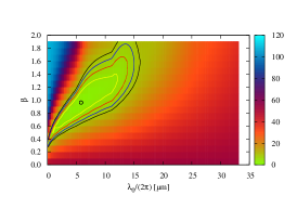
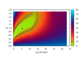
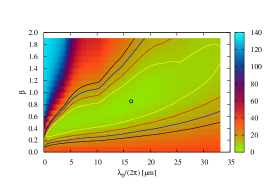
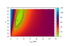
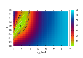
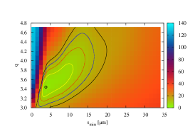
Figure 7.— The $\chi^{2}$-maps for HD 50571 (left), HD 195627 (middle), and Fomalhaut (right) in the MBB (top) and SD (bottom) method. The lines show the $n\cdot\chi^{2}_{\text{red}}$ isolines for $n=1$ (small circle), $n=2$ (yellow line), $n=3$ (red line), $n=4$ (blue line) and $n=5$ (black line), where $\chi^{2}_{\text{red}}$ is the best-fit value.

Figure 7 presents typical $\chi^{2}$-maps for three stars with different luminosities, obtained with both fitting methods. The contours of equal $\chi^{2}$ are elongated from the bottom left to the top right, which is easy to understand. Indeed, when $\lambda_{0}$ (or $s_{\mathrm{min}}$) is larger than the best-fit value, the fitting routine tries to compensate it by taking a steeper size distribution, with a larger $\beta$ (or $q$). Not only the bottom left – top right orientation, but also the shape of the isolines can be better understood with the following arguments. We take the SD method as an example. Assuming that the emission of the different-sized grains is proportional to their cross section (which is only a rough approximation to reality, of course), we can define the “effective” grain size, $s_{0}$. The effective grain size is the one in which we replace the grains with a size distribution (4) with the same number of equal-sized grains of radius $s_{0}$, requiring that the latter have the same total cross section. This gives

$$\int\limits_{s_{\mathrm{min}}}^{\infty}s^{2-q}ds=s_{0}^{2}\int\limits_{s_{\mathrm{min}}}^{\infty}s^{-q}ds.$$ (B1)

For $q>3$, this results in

$$s_{0}\approx s_{\mathrm{min}}\;\sqrt{(q-1)/(q-3)},$$ (B2)

so that, for instance, $q=3.5$ corresponds to $s_{0}\approx 2.2s_{\mathrm{min}}$. We can expect that different pairs $(s_{\mathrm{min}},q)$ with the same $s_{0}$ should lead to SEDs that reproduce the observed one equally well. In other words, the isolines of $\chi^{2}$ should roughly follow the equation

$$s_{\mathrm{min}}\;\sqrt{(q-1)/(q-3)}=\text{const}.$$ (B3)

The shape of the $q(s_{\mathrm{min}})$ curve determined by Eq. (B3) is exactly the one that is seen in Figure 7. In particular, $q$ rises more steeply at larger $s_{\mathrm{min}}$ (a banana shape best seen in yellow- and red-filled regions corresponding to moderate $\chi^{2}$ values). We can also explain why the tilt of the isolines to the x-axis gets smaller for stars of higher luminosities (i.e. from the left to the right panels of Figure 7). This is because $s_{0}$ is larger around those stars, so that at the same $s_{\mathrm{min}}$ the derivative $dq/ds_{\mathrm{min}}$ is smaller.

References

- Acke et al. (2012) Acke, B., Min, M., Dominik, C., et al. 2012, A& A, 540, A125
- Allende Prieto et al. (1999) Allende Prieto, C., García López, R. J., Lambert, D. L., & Gustafsson, B. 1999, ApJ, 527, 879
- Backman & Paresce (1993) Backman, D., & Paresce, F. 1993, in Protostars and Planets III, ed. E. H. Levy & J. I. Lunine (Univ. of Arizona Press), 1253–1304
- Backman et al. (2009) Backman, D., Marengo, M., Stapelfeldt, K., et al. 2009, ApJ, 690, 1522
- Ballering et al. (2013) Ballering, N. P., Rieke, G. H., Su, K. Y. L., & Montiel, E. 2013, ApJ, 775, 55
- Balog et al. (2013) Balog, Z., Müller, T., Nielbock, M., et al. 2013, Experimental Astronomy, arXiv:1309.6099
- Bessell (1979) Bessell, M. S. 1979, PASP, 91, 589
- Boley et al. (2012) Boley, A. C., Payne, M. J., Corder, S., et al. 2012, ApJ, 750, L21
- Bonsor et al. (2013) Bonsor, A., Kennedy, G. M., Crepp, J. R., et al. 2013, MNRAS, 431, 3025
- Booth et al. (2013) Booth, M., Kennedy, G., Sibthorpe, B., et al. 2013, MNRAS, 428, 1263
- Broekhoven-Fiene et al. (2013) Broekhoven-Fiene, H., Matthews, B. C., Kennedy, G. M., et al. 2013, ApJ, 762, 52
- Brott & Hauschildt (2005) Brott, I., & Hauschildt, P. H. 2005, in ESA SP, Vol. 576, The Three-Dimensional Universe with Gaia, ed. C. Turon, K. S. O’Flaherty, & M. A. C. Perryman, 565
- Burns et al. (1979) Burns, J. A., Lamy, P. L., & Soter, S. 1979, Icarus, 40, 1
- Castelli & Kurucz (2004) Castelli, F., & Kurucz, R. L. 2004, ArXiv:astro-ph/0405087
- Chen et al. (2014) Chen, C. H., Mittal, T., Kuchner, M., et al. 2014, ApJS, 211, 25
- Chen et al. (2012) Chen, C. H., Pecaut, M., Mamajek, E. E., Su, K. Y. L., & Bitner, M. 2012, ApJ, 756, 133
- Churcher et al. (2011) Churcher, L., Wyatt, M., & Smith, R. 2011, MNRAS, 410, 2
- Cohen et al. (2003) Cohen, M., Wheaton, W. A., & Megeath, S. T. 2003, AJ, 126, 1090
- Cutri et al. (2003) Cutri, R. M., Skrutskie, M. F., van Dyk, S., et al. 2003, 2MASS All Sky Catalog of point sources.
- Dodson-Robinson et al. (2009) Dodson-Robinson, S. E., Willacy, K., Bodenheimer, P., Turner, N. J., & Beichman, C. A. 2009, Icarus, 200, 672
- Dohnanyi (1969) Dohnanyi, J. S. 1969, J. Geophys. Res., 74, 2531
- Donaldson et al. (2013) Donaldson, J. K., Lebreton, J., Roberge, A., Augereau, J.-C., & Krivov, A. V. 2013, ApJ, 772, 17
- Draine (2003) Draine, B. T. 2003, ARA& A, 41, 241
- Duchêne et al. (2014) Duchêne, G., Arriaga, P., Wyatt, M., et al. 2014, ApJ, 784, 148
- Dutrey et al. (2014) Dutrey, A., Semenov, D., Chapillon, E., et al. 2014, in Protostars and Planets VI, ed. H. Beuther, R. Klessen, C. Dullemond, & T. Henning (Univ. of Arizona Press), in press, arXiv:1402.3503
- Eiroa et al. (2013) Eiroa, C., Marshall, J. P., Mora, A., et al. 2013, A& A, 555, A11
- Ertel et al. (2011) Ertel, S., Wolf, S., Metchev, S., et al. 2011, A& A, 533, A132
- Ertel et al. (2014) Ertel, S., Marshall, J. P., Augereau, J.-C., et al. 2014, A& A, 561, A114
- Farihi et al. (2009) Farihi, J., Jura, M., & Zuckerman, B. 2009, ApJ, 694, 805
- Frisch et al. (2011) Frisch, P. C., Redfield, S., & Slavin, J. D. 2011, ARA& A, 49, 237
- Gänsicke et al. (2006) Gänsicke, B. T., Marsh, T. R., Southworth, J., & Rebassa-Mansergas, A. 2006, Science, 314, 1908
- Golimowski et al. (2006) Golimowski, D. A., Ardila, D. R., Krist, J. E., et al. 2006, AJ, 131, 3109
- Gray (1992) Gray, D. F. 1992, The observation and analysis of stellar photospheres., ed. Gray, D. F.
- Gray et al. (2006) Gray, R. O., Corbally, C. J., Garrison, R. F., et al. 2006, AJ, 132, 161
- Gray et al. (2003) Gray, R. O., Corbally, C. J., Garrison, R. F., McFadden, M. T., & Robinson, P. E. 2003, AJ, 126, 2048
- Griffin et al. (2010) Griffin, M. J., Abergel, A., Abreu, A., et al. 2010, A& A, 518, L3
- Holmberg et al. (2009) Holmberg, J., Nordström, B., & Andersen, J. 2009, A& A, 501, 941
- Ishihara et al. (2010) Ishihara, D., Onaka, T., Kataza, H., et al. 2010, A&A, 514, A1
- Johansen et al. (2014) Johansen, A., Blum, J., Tanaka, H., et al. 2014, in Protostars and Planets VI, ed. H. Beuther, R. Klessen, C. Dullemond, & T. Henning (Univ. of Arizona Press), in press, arXiv:1402.1344
- Kennedy & Wyatt (2010) Kennedy, G. M., & Wyatt, M. C. 2010, MNRAS, 405, 1253
- Kennedy et al. (2012) Kennedy, G. M., Wyatt, M. C., Sibthorpe, B., et al. 2012, MNRAS, 426, 2115
- Kenyon & Bromley (2008) Kenyon, S. J., & Bromley, B. C. 2008, ApJS, 179, 451
- Kirchschlager & Wolf (2013) Kirchschlager, F., & Wolf, S. 2013, A&A, 552, A54
- Kobayashi et al. (2011) Kobayashi, H., Tanaka, H., & Krivov, A. V. 2011, ApJ, 738, 35
- Krijt & Kama (2014) Krijt, S., & Kama, M. 2014, A& A, 566, L2
- Krist et al. (2012) Krist, J. E., Stapelfeldt, K. R., Bryden, G., & Plavchan, P. 2012, AJ, 144, 45
- Krivov et al. (2006) Krivov, A. V., Löhne, T., & Sremčević, M. 2006, A& A, 455, 509
- Krivov et al. (2008) Krivov, A. V., Müller, S., Löhne, T., & Mutschke, H. 2008, ApJ, 687, 608
- Krivov et al. (2013) Krivov, A. V., Eiroa, C., Löhne, T., et al. 2013, ApJ, 772, 32
- Kuchner & Stark (2010) Kuchner, M. J., & Stark, C. C. 2010, AJ, 140, 1007
- Lebouteiller et al. (2011) Lebouteiller, V., Barry, D. J., Spoon, H. W. W., et al. 2011, ApJS, 196, 8
- Lebreton et al. (2012) Lebreton, J., Augereau, J.-C., Thi, W.-F., et al. 2012, A& A, 539, A17
- Lebreton et al. (2013) Lebreton, J., van Lieshout, R., Augereau, J.-C., et al. 2013, A& A, 555, A146
- Lestrade et al. (2012) Lestrade, J.-F., Matthews, B. C., Sibthorpe, B., et al. 2012, A& A, 548, A86
- Liseau et al. (2008) Liseau, R., Risacher, C., Brandeker, A., et al. 2008, A& A, 480, L47
- Liseau et al. (2010) Liseau, R., Eiroa, C., Fedele, D., et al. 2010, A& A, 518, L132
- Löhne et al. (2008) Löhne, T., Krivov, A. V., & Rodmann, J. 2008, ApJ, 673, 1123
- Löhne et al. (2012) Löhne, T., Augereau, J.-C., Ertel, S., et al. 2012, A& A, 537, A110
- Marshall et al. (2011) Marshall, J. P., Löhne, T., Montesinos, B., et al. 2011, A& A, 529, A117
- Matthews et al. (2014a) Matthews, B., Kennedy, G., Sibthorpe, B., et al. 2014a, ApJ, 780, 97
- Matthews et al. (2014b) Matthews, B. C., Krivov, A. V., Wyatt, M. C., Bryden, G., & Eiroa, C. 2014b, in Protostars and Planets VI, ed. H. Beuther, R. Klessen, C. Dullemond, & T. Henning (U. Arizona Press), in press, arXiv:1401.0743
- Matthews et al. (2010) Matthews, B. C., Sibthorpe, B., Kennedy, G., et al. 2010, A& A, 518, L135
- Moór et al. (2011) Moór, A., Ábrahám, P., Juhász, A., et al. 2011, ApJL, 740, L7
- Moór et al. (2013a) Moór, A., Ábrahám, P., Kóspál, Á., et al. 2013a, ApJL, 775, L51
- Moór et al. (2013b) Moór, A., Juhász, A., Kóspál, Á., et al. 2013b, ApJL, 777, L25
- Morales et al. (2013) Morales, F. Y., Bryden, G., Werner, M. W., & Stapelfeldt, K. R. 2013, ApJ, 776, 111
- Morales et al. (2011) Morales, F. Y., Rieke, G. H., Werner, M. W., et al. 2011, ApJL, 730, L29
- Morales et al. (2009) Morales, F. Y., Werner, M. W., Bryden, G., et al. 2009, ApJ, 699, 1067
- Müller et al. (2010) Müller, S., Löhne, T., & Krivov, A. V. 2010, ApJ, 708, 1728
- Mustill & Wyatt (2009) Mustill, A. J., & Wyatt, M. C. 2009, MNRAS, 399, 1403
- Najita & Williams (2005) Najita, J., & Williams, J. P. 2005, ApJ, 635, 625
- Nilsson et al. (2010) Nilsson, R., Liseau, R., Brandeker, A., et al. 2010, A& A, 518, A40
- Ott (2010) Ott, S. 2010, in ASP Conf. Series, Vol. 434, Astronomical Data Analysis Software and Systems XIX, ed. Y. Mizumoto, K.-I. Morita, & M. Ohishi, 139
- Paunzen et al. (2006) Paunzen, E., Schnell, A., & Maitzen, H. M. 2006, A&A, 458, 293
- Pilbratt et al. (2010) Pilbratt, G. L., Riedinger, J. R., Passvogel, T., et al. 2010, A& A, 518, L1
- Plavchan et al. (2005) Plavchan, P., Jura, M., & Lipscy, S. J. 2005, ApJ, 631, 1161
- Poglitsch et al. (2010) Poglitsch, A., Waelkens, C., Geis, N., et al. 2010, A& A, 518, L2
- Press et al. (2002) Press, W. H., Teukolsky, S. A., Vetterling, W. T., & Flannery, B. P. 2002, Numerical Recipes in C++ (Cambridge University Press), 1032 pp.
- Raymond et al. (2011) Raymond, S. N., Armitage, P. J., Moro-Martín, A., et al. 2011, A& A, 530, A62
- Reidemeister et al. (2011) Reidemeister, M., Krivov, A. V., Stark, C. C., et al. 2011, A& A, 527, A57
- Reis et al. (2011) Reis, W., Corradi, W., de Avillez, M. A., & Santos, F. P. 2011, ApJ, 734, 8
- Rieke & Lebofsky (1985) Rieke, G. H., & Lebofsky, M. J. 1985, ApJ, 288, 618
- Roberge et al. (2006) Roberge, A., Feldman, P. D., Weinberger, A. J., Deleuil, M., & Bouret, J.-C. 2006, Nature, 441, 724
- Roberge et al. (2013) Roberge, A., Kamp, I., Montesinos, B., et al. 2013, ApJ, 771, 69
- Rodriguez & Zuckerman (2012) Rodriguez, D. R., & Zuckerman, B. 2012, ApJ, 745, 147
- Ros & Johansen (2013) Ros, K., & Johansen, A. 2013, A& A, 552, A137
- Sheret et al. (2004) Sheret, I., Dent, W. R. F., & Wyatt, M. C. 2004, MNRAS, 348, 1282
- Sibthorpe et al. (2010) Sibthorpe, B., Vandenbussche, B., Greaves, J. S., et al. 2010, A& A, 518, L130
- Stock et al. (2010) Stock, N. D., Su, K. Y. L., Liu, W., et al. 2010, ApJ, 724, 1238
- Su et al. (2005) Su, K. Y. L., Rieke, G. H., Misselt, K. A., et al. 2005, ApJ, 628, 487
- Su et al. (2006) Su, K. Y. L., Rieke, G. H., Stansberry, J. A., et al. 2006, ApJ, 653, 675
- Su et al. (2009) Su, K. Y. L., Rieke, G. H., Stapelfeldt, K. R., et al. 2009, ApJ, 705, 314
- Su et al. (2013) Su, K. Y. L., Rieke, G. H., Malhotra, R., et al. 2013, ApJ, 763, 118
- Thébault & Augereau (2007) Thébault, P., & Augereau, J.-C. 2007, A& A, 472, 169
- Thébault & Wu (2008) Thébault, P., & Wu, Y. 2008, A& A, 481, 713
- Torres (2010) Torres, G. 2010, AJ, 140, 1158
- Trilling et al. (2007) Trilling, D. E., Stansberry, J. A., Stapelfeldt, K. R., et al. 2007, ApJ, 658, 1289
- Vitense et al. (2010) Vitense, C., Krivov, A. V., & Löhne, T. 2010, A& A, 520, A32
- von Braun et al. (2011) von Braun, K., Boyajian, T. S., Kane, S. R., et al. 2011, ApJL, 729, L26
- Wahhaj et al. (2007) Wahhaj, Z., Koerner, D. W., & Sargent, A. I. 2007, ApJ, 661, 368
- Williams & Andrews (2006) Williams, J. P., & Andrews, S. M. 2006, ApJ, 653, 1480
- Williams & Cieza (2011) Williams, J. P., & Cieza, L. A. 2011, ARA& A, 49, 67
- Wright et al. (2010) Wright, E. L., Eisenhardt, P. R. M., Mainzer, A. K., et al. 2010, AJ, 140, 1868
- Wyatt (2008) Wyatt, M. C. 2008, ARA& A, 46, 339
- Wyatt et al. (2011) Wyatt, M. C., Clarke, C. J., & Booth, M. 2011, Celest. Mech. Dynam. Astron., 111, 1
- Wyatt et al. (2012) Wyatt, M. C., Kennedy, G., Sibthorpe, B., et al. 2012, MNRAS, 424, 1206
- Zuckerman et al. (2003) Zuckerman, B., Koester, D., Reid, I. N., & Hünsch, M. 2003, ApJ, 596, 477