Sparse Quadratic Discriminant Analysis
and Community Bayes

Abstract

We develop a class of rules spanning the range between quadratic discriminant analysis and naive Bayes, through a path of sparse graphical models. A group lasso penalty is used to introduce shrinkage and encourage a similar pattern of sparsity across precision matrices. It gives sparse estimates of interactions and produces interpretable models. Inspired by the connected-components structure of the estimated precision matrices, we propose the community Bayes model, which partitions features into several conditional independent communities and splits the classification problem into separate smaller ones. The community Bayes idea is quite general and can be applied to non-Gaussian data and likelihood-based classifiers.

1 Introduction

In the generic classification problem, the outcome of interest $G$ falls into $K$ unordered classes, which for convenience we denote by $\{1,2,\ldots,K\}$. Our goal is to build a rule for predicting the class label of an item based on $p$ measurements of features $X\in\mathbb{R}^{p}$. The training set consists of the class labels and features for $n$ items. This is an important practical problem with applications in many fields.

Quadratic discriminant analysis (QDA) can be derived as the maximum likelihood method for normal populations with different means and different covariance matrices. It is a favored tool when there are some strong interactions and linear boundaries cannot separate the classes. However, QDA is poorly posed when the sample size $n_{k}$ is not considerably larger than $p$ for any class $k$, and clearly ill-posed if $n_{k}\leq p$. Therefore it encourages us to employ a regularization method [17, 24]. Although there already exist a number of proposals to regularize linear discriminant analysis (LDA) [1, 4, 6, 8, 9, 11, 23, 26], few methods have been developed to regularize QDA. Friedman [7] suggests applying a ridge penalty to within-class covariance matrices, and Price et al. [19] propose to add a ridge penalty and a ridge fusion penalty to the log-likelihood. For both methods, no elements of the resulting within-class precision matrices will be zero, leading to dense interaction terms in the discriminant functions and difficulties in interpretation. Assuming sparse conditions on both unknown means and covariance matrices, Li and Shao [13] propose to construct mean and covariance estimators by thresholding. Sun and Zhao [21] assume block-diagonal structure for covariance matrices and estimate each block by $l_{1}$ regularization. The blocks are assumed to be of the same size, and are formed based on two sample $t$ statistics. However, both methods can only apply to two-class classification. Another approach is to assume conditional independence of the features (naive Bayes). Naive Bayes classifiers often outperform far more sophisticated alternatives when the dimension $p$ of the feature space is high , but the conditional independence assumption may be too rigid in the presence of strong interactions.

In this paper we develop a class of rules spanning the range between QDA and naive Bayes using a group lasso penalty [27]. A group lasso penalty is applied to the $(i,j)$th element across all $K$ within-class precision matrices, which forces the zeros in the $K$ estimated precision matrices to occur in the same places. This shared pattern of sparsity results in a sparse estimate of interaction terms, making the classifier easy to interpret. We refer to this classification method as Sparse Quadratic Discriminant Analysis (SQDA).

The connected components in the resulting precision matrices correspond exactly to those obtained from simple thresholding rules on the within-class sample covariance matrices [5]. This suggests us to partition features into several independent communities before estimating the parameters [3, 10, 18].

Therefore, we propose the community Bayes model, a simple idea to identify and make use of conditional independent communities of features. Furthermore, it is a general approach applicable to non-Gaussian data and any likelihood-based classifiers. Specifically, the community Bayes works by partitioning features into several communities, solving separate classification problems for each community, and combining the community-wise results into one final prediction. We show that this approach can improve the accuracy and interpretability of the corresponding classifier.

The paper is organized as follows. In section 2 we discuss sparse quadratic discriminant analysis and the sample covariance thresholding rules. In section 3 we discuss the community Bayes idea. Simulated and real data examples appear in Section 4, concluding remarks in Section 5 and the proofs are gathered in the Appendix.

2 Sparse Quadratic Discriminant Analysis

Suppose we have training data $(x_{i},g_{i})\in\mathbb{R}^{p}\times K$, $i=1,2,\ldots,n$, where $x_{i}$’s are observations with measurements on a set of $p$ features and $g_{i}$’s are class labels. We assume that the $n_{k}$ observations within the $k$th class are identically distributed as $N(\mu_{k},\mathbf{\Sigma}_{k})$, and the $n=\sum_{k}n_{k}$ observations are independent. We let $\pi_{k}$ denote the prior for class $k$. Then the quadratic discriminant function is

$$\delta_{k}(x)=\frac{1}{2}\log\mbox{det }\mathbf{\Sigma}_{k}^{-1}-\frac{1}{2}(x-\mu_{k})^{T}\mathbf{\Sigma}_{k}^{-1}(x-\mu_{k})+\log\pi_{k}.$$ (1)

Let $\mathbf{\Theta}^{(k)}=\mathbf{\Sigma}_{k}^{-1}$ denote the true precision matrix for class $k$, and $\theta_{ij}=(\theta_{ij}^{(1)},\ldots,\theta_{ij}^{(K)})$ denote the vector of the $(i,j)$th element across all $K$ precision matrices. We propose to estimate $\mu,\pi,\mathbf{\Theta}$ by maximizing the penalized log likelihood

$$\sum_{k=1}^{K}\left[\frac{n_{k}}{2}\log\text{det }\mathbf{\Theta}^{(k)}-\frac{1}{2}\sum_{g_{i}=k}(x_{i}-\mu_{k})^{T}\mathbf{\Theta}^{(k)}(x_{i}-\mu_{k})+n_{k}\log\pi_{k}\right]-\frac{\lambda}{2}\sum_{i\neq j}\|\theta_{ij}\|_{2}.$$ (2)

The last term is a group lasso penalty, applied to the $(i,j)$th element across all $K$ precision matrices, which forces a similar pattern of sparsity across all the precision matrices. Hence, we refer to this classification method as Sparse Quadratic Discriminant Analysis (SQDA).

Let $\mathbf{\Theta}=(\mathbf{\Theta}^{(1)},\ldots,\mathbf{\Theta}^{(K)})$. Solving (2) gives us the estimates

$$\hat{\mu}_{k}= \frac{1}{n_{k}}\sum_{g_{i}=k}x_{i}$$ (3)

$$\hat{\pi}_{k}= \frac{n_{k}}{n}$$ (4)

$$\hat{\mathbf{\Theta}}= \mbox{argmax}_{\mathbf{\Theta}^{(k)}\succ 0}\sum_{k=1}^{K}n_{k}\left(\log\text{det }\mathbf{\Theta}^{(k)}-\text{tr}(\mathbf{S}^{(k)}\mathbf{\Theta}^{(k)})\right)-\lambda\sum_{i\neq j}\|\theta_{ij}\|_{2},$$ (5)

where $\mathbf{S}^{(k)}=\frac{1}{n_{k}}\sum_{g_{i}=k}(x_{i}-\hat{\mu}_{k})(x_{i}-\hat{\mu}_{k})^{T}$ is the sample covariance matrix for class $k$.

This model has several important features:

1. $\lambda$ is a nonnegative tuning parameter controlling the simultaneous shrinkage of all precision matrices toward diagonal matrices. The value $\lambda=0$ gives rise to QDA, whereas $\lambda=\infty$ yields the naive Bayes classifier. Values between these limits represent degrees of regularization less severe than naive Bayes. Since it is often the case that even small amounts of regularization can largely eliminate quite drastic instability, smaller values of $\lambda$ (smaller than $\infty$) have the potential of superior performance when some features have strong partial correlations.

2. The group lasso penalty forces $\hat{\mathbf{\Theta}}^{(1)},\ldots,\hat{\mathbf{\Theta}}^{(K)}$ to share the locations of the nonzero elements, leading to a sparse estimate of interactions. Therefore, our method produces more interpretable results.

3. The optimization problem (5) can be separated into independent sub-problems of the same form by simple screening rules on $\mathbf{S}^{(1)},\ldots,\mathbf{S}^{(K)}$. This leads to a potentially massive reduction in computational complexity.

The convex optimization problem (5) can be quickly solved by R package JGL [5]. Not for the purpose of classification as here, Danaher et al. [5] propose to jointly estimate multiple related Gaussian graphical models by maximizing the group graphical lasso

$$\mbox{max}_{\mathbf{\Theta}^{(k)}\succ 0}\sum_{k=1}^{K}n_{k}\left(\log\mbox{det}\mathbf{\Theta}^{(k)}-\mbox{tr}(\mathbf{S}^{(k)}\mathbf{\Theta}^{(k)})\right)-\lambda_{1}\sum_{i\neq j}\|\theta_{ij}\|_{1}-\lambda_{2}\sum_{i\neq j}\|\theta_{ij}\|_{2}.$$ (6)

They use the additional lasso penalty to further encourage sparsity within $(\theta_{ij}^{(1)},\ldots,\theta_{ij}^{(K)})$. However, for the purpose of classification, our goal is to identify interaction terms – that is, we are interested in whether $(\theta_{ij}^{(1)},\ldots,\theta_{ij}^{(K)})$ is a zero vector instead of whether each element $\theta_{ij}^{(k)}$ is zero. Therefore, we only use the group lasso penalty to estimate precision matrices.

We illustrate our method with a handwritten digit recognition example. Here we focus on the sub-task of distinguishing handwritten 3s and 8s. We use the same data as Le Cun et al. [12], who normalized binary images for size and orientation, resulting in 8-bit, $16\times 16$ gray scale images. There are 658 threes and 542 eights in our training set, and 166 test samples for each. Figure 1 shows a random selection of 3s and 8s.

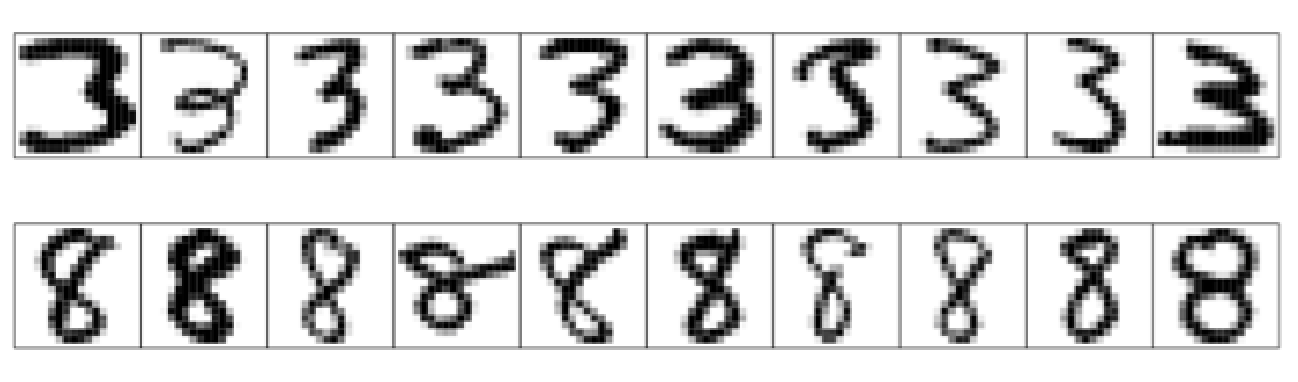
Figure 1: Examples of digitized handwritten 3s and 8s. Each image is a 8 bit, $16\times 16$ gray scale version of the original binary image.

Because of their spatial arrangement the features are highly correlated and some kind of smoothing or filtering always helps. We filtered the data by replacing each non-overlapping $2\times 2$ pixel block with its average. This reduces the dimension of the feature space from 256 to 64.

We compare our method with QDA, naive Bayes and a variant of RDA which we refer to as diagonal regularized discriminant analysis (DRDA). The estimated covariance matrix of DRDA for class $k$ is

$$\hat{\mathbf{\Sigma}}^{(k)}(\lambda)=(1-\lambda)\mathbf{S}^{(k)}+\lambda\mbox{diag}(\mathbf{S}^{(k)}),\mbox{ with }\lambda\in[0,1].$$ (7)

The tuning parameters are selected by 5-fold cross validation. Table 1 shows the misclassification errors of each method and the corresponding standardized tuning parameters $s=P(\hat{\mathbf{\Theta}}(\lambda))/P(\hat{\mathbf{\Theta}}(0))$, where $P(\mathbf{\Theta})=\Sigma_{i\neq j}||\theta_{ij}^{(1)},\ldots,\theta_{ij}^{(K)}||_{2}$. The results show that SQDA outperforms DRDA, QDA and naive Bayes. In Figure 3, we see that the test error of SQDA decreases dramatically as the model deviates from naive Bayes and achieves its minimum at a small value of $s$, while the test error of DRDA keeps decreasing as the model ranges from naive Bayes to QDA. This is expected since at small values of $s$, SQDA only includes important interaction terms and shrinks other noisy terms to 0, but DRDA has all interactions in the model once deviating from naive Bayes. To better display the estimated precision matrices, we standardize the estimates to have unit diagonal (the standardized precision matrix is equal to the partial correlation matrix up to the sign of off-diagonal entries). Figure 3 displays the standardized sample precision matrices, and the standardized SQDA and DRDA estimates. From Figure 3, we can see that SQDA only includes interactions within a diagonal band.

Table 1: Digit classification results of 3s and 8s. Tuning parameters are selected by 5-fold cross validation.

	SQDA	DRDA	QDA	Naive Bayes
Test error	0.042	0.063	0.063	0.160
Training error	0.024	0.024	0.022	0.119
CV error	0.028	0.043	–	–
Standardized tuning parameter	0.016	0.760	–	–

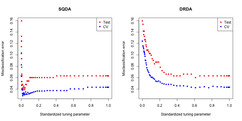
Figure 2: The 5-fold cross-validation errors (blue) and the test errors (red) of SQDA and DRDA on 3s and 8s.

Figure 3: Heat maps of the sample precision matrices and the estimated precision matrices of SQDA and DRDA. Estimates are standardized to have unit diagonal. The first line corresponds to the precision matrix of 3s and the second line corresponds to that of 8s.

2.1 Exact covariance thresholding into connected components

Mazumder & Hastie [16] and Witten et al. [25] establish a connection between the graphical lasso and connected components. Specifically, the connected components in the estimated precision matrix correspond exactly to those obtained from thresholding the entries of the sample covariance matrix at $\lambda$. For the solution to (5), we have similar results. By simple thresholding rules on the sample covariance matrices $\mathbf{S}^{(1)},\ldots,\mathbf{S}^{(K)}$, the optimization problem (5) can be separated into several optimization sub-problems of the same form, which leads to huge speed improvements. A more general result for the solution to (6) can be found in [5].

Suppose $\hat{\mathbf{\Theta}}=(\hat{\mathbf{\Theta}}^{(1)},\ldots,\hat{\mathbf{\Theta}}^{(K)})$ is the solution to (5) with regularization parameter $\lambda$. Define

$$\mathcal{\mathbf{\mathcal{E}}}_{ij}^{(\lambda)}=\begin{cases}1&\mbox{if}\ (\hat{\theta}_{ij}^{(1)},\ldots,\hat{\theta}_{ij}^{(K)})\neq\vec{\mathbf{0}},\ i\neq j;\\ 0&\mbox{otherwise}.\end{cases}$$ (8)

This defines a symmetric graph $\mathcal{G}^{(\lambda)}=(\mathcal{V},\mathcal{\mathbf{\mathcal{E}}}^{(\lambda)})$, namely the estimated concentration graph defined on the nodes $\mathcal{V}=\{1,\ldots,p\}$ with edges $\mathbf{\mathcal{E}}^{(\lambda)}$. Suppose it admits a decomposition into $\kappa(\lambda)$ connected components

$$\mathcal{G}^{(\lambda)}=\cup_{l=1}^{\mathbf{\kappa}(\lambda)}\mathcal{G}_{l}^{(\lambda)},$$ (9)

where $\mathcal{\mathcal{G}}_{l}^{(\lambda)}=(\hat{\mathcal{V}}_{l}^{(\lambda)},\mathbf{\mathcal{E}}_{l}^{(\lambda)})$ are the components of the graph $\mathcal{G}^{(\lambda)}$.

Define $\tilde{\mathbf{S}}_{ij}=||(n_{1}\mathbf{S}_{ij}^{(1)},\ldots,n_{K}\mathbf{S}_{ij}^{(K)})||_{2}$.We can also perform a thresholding on the entries of $\tilde{\mathbf{S}}$ and obtain a graph edge skeleton defined by

$$\mathbf{E}_{ij}^{(\lambda)}=\begin{cases}1&\mbox{if}\ \tilde{\mathbf{S}}_{ij}>\lambda,\ i\neq j;\\ 0&\mbox{otherwise}.\end{cases}$$ (10)

The symmetric matrix $\mathbf{E}^{(\lambda)}$ defines a symmetric graph $\mathrm{G}^{(\lambda)}=(\mathcal{V},\mathbf{E}^{(\lambda)})$, which is referred to as the thresholded sample covariance graph. $\mathrm{G}^{(\lambda)}$ also admits a decomposition into connected components

$$\mathrm{G}^{(\lambda)}=\cup_{l=1}^{k(\lambda)}\mathrm{G}_{l}^{(\lambda)},$$ (11)

where $\mathrm{G}_{l}^{(\lambda)}=(\mathcal{V}_{l}^{(\lambda)},\mathbf{E}_{l}^{(\lambda)})$ are the components of the graph $\mathbf{G}^{(\lambda)}$.

Theorem 1.

For any $\lambda>0$, the components of the estimated concentration graph $\mathcal{G}^{(\lambda)}$ induce exactly the same vertex-partition as that of the thresholded sample covariance graph $\mathrm{G}^{(\lambda)}$. Formally, $\kappa(\lambda)=k(\lambda)$ and there exists a permutation $\pi$ on $\{1,\ldots,k(\lambda)\}$ such that

$$\hat{\mathcal{V}}_{i}^{(\lambda)}=\mathcal{V}_{\pi(i)}^{(\lambda)},\ \forall i=1,\ldots,k(\lambda).$$ (12)

Furthermore, given $\lambda>\lambda^{\prime}>0$, the vertex-partition induced by the components of $\mathcal{G}^{(\lambda)}$ are nested within that induced by the components of $\mathcal{G}^{(\lambda^{\prime})}$. That is, $\kappa(\lambda)\geq\kappa(\lambda^{\prime})$ and the vertex-partition $\{\hat{\mathcal{V}}_{l}^{(\lambda)}\}_{1\leq l\leq\kappa(\lambda)}$ forms a finer resolution of $\{\hat{\mathcal{V}}_{l}^{(\lambda^{\prime})}\}_{1\leq l\leq\kappa(\lambda^{\prime})}$.

Proof.

The proof of this theorem appears in the Appendix. ∎

Theorem 1 allows us to quickly check the connected components of the estimated concentration graph by simple screening rules on $\tilde{\mathbf{S}}$. Notice that for each class $k$, the edge set $\mathbf{\mathcal{E}}^{(k,\lambda)}$ defined by $\mathbf{\mathcal{E}}_{ij}^{(k,\lambda)}=\mathbf{1}_{\{\hat{\theta}_{ij}^{(k)}\neq 0\}}$ is nested in $\mathbf{\mathcal{E}}^{(\lambda)}$. Therefore, the features can be reordered in such a way that each $\hat{\mathbf{\Theta}}^{(k)}$ is block diagonal

$$\hat{\mathbf{\Theta}}^{(k)}=\left(\begin{array}[]{cccc}\hat{\mathbf{\Theta}}_{1}^{(k)}&0&\cdots&0\\ 0&\hat{\mathbf{\Theta}}_{2}^{(k)}&0&\cdots\\ \vdots&\vdots&\ddots&\vdots\\ 0&\cdots&0&\hat{\mathbf{\Theta}}_{k(\lambda)}^{(k)}\end{array}\right),$$ (13)

where the different components represent blocks of indices given by $\mathcal{V}_{l}^{(\lambda)},\ l=1,\ldots,k(\lambda)$. Then one can simply solve the optimization problem (5) on the features within each block separately, making problem (5) feasible for certain values of $\lambda$ although it may be impossible to operate on the $p\times p$ variables $\mathbf{\Theta}^{(1)},\ldots,\mathbf{\Theta}^{(K)}$ on a single machine.

3 Community Bayes

The estimated precision matrices of SQDA are often block diagonal under suitable ordering of the features, which implies that the features can be partitioned into several communities and these communities are mutually independent within each class. In this section, we generalize this idea to non-Gaussian data and other classification models, and refer to it as the community Bayes model. A related work in the regression setting is [10]. The authors propose to split the lasso problem into smaller ones by estimating the connected components of the sample covariance matrix. Their approach involves only one covariance matrix and works specifically for the lasso.

3.1 Main idea

We let $X\in\mathbb{R}^{p}$ denote the feature vector and $G\in\{1,\ldots,K\}$ denote the class variable. Suppose the feature set $\mathcal{V}=\{1,\ldots,p\}$ admits a partition $\mathcal{V}=\cup_{l=1}^{L}\mathcal{V}_{l}$ such that $X_{\mathcal{\mathcal{V}}_{1}},\ldots,X_{\mathcal{V}_{L}}$ are mutually independent conditional on $G=k$ for $k=1,\ldots,K$, where $X_{\mathcal{V}_{l}}$ is a subset of $X$ containing the features in community $\mathcal{V}_{l}$. Then the posterior probability has the form

$$\log p(G=k|X) = \log p(X|G=k)+\log p(G=k)-\log p(X)$$ (14)

$$= \sum_{l=1}^{L}\log p(X_{\mathcal{V}_{l}}|G=k)+\log p(G=k)-\log p(X)$$ (15)

$$= \sum_{l=1}^{L}\log p(G=k|X_{\mathcal{V}_{l}})+(1-L)\log p(G=k)+C(X)$$ (16)

where $C(X)=\sum_{l=1}^{L}\log p(X_{\mathcal{V}_{l}})-\log p(X)$ only depends on $X$ and serves as a normalization term.

The equation (16) implies an interesting result: we can fit the classification model on each community separately, and combine the resultant posteriors into the posterior to the original problem by simply adjusting the intercept and normalizing it. This result has three important consequences:

1. The global problem completely separates into $L$ smaller tractable sub-problems of the same form, making it possible to solve an otherwise infeasible large-scale problem. Moreover, the modular structure lends it naturally to parallel computation. That is, one can solve these sub-problems independently on separate machines.

2. This idea is quite general and can be applied to any likelihood-based classifiers, including discriminant analysis, multinomial logistic regression, generalized additive models, classification trees, etc.

3. When using a classification model with interaction terms, (16) doesn’t involve interactions across different communities. Therefore, it has fewer degrees of freedom and thus smaller variance than the global problem.

To find conditionally independent communities, we use the Spearman’s rho, a robust nonparametric rank-based statistics, to directly estimate the unknown correlation matrices, and then apply average, single or complete linkage clustering to the estimated correlation matrices to get the estimated communities. In next section, we will show that this procedure consistently identify conditionally independent communities when the data are from a nonparanormal family.

The community Bayes algorithm is summarized below.

Algorithm 1 The community Bayes algorithm

1:  Compute $\hat{\mathbf{R}}^{(k)}$, the estimated correlation matrix based on the Spearman’s rho for each class $k$.

2:  Perform average, single or complete linkage clustering with similarity matrix $\tilde{\mathbf{R}}$, where $\tilde{\mathbf{R}}_{ij}=||(n_{1}\hat{\mathbf{R}}_{ij}^{(1)},\ldots,n_{K}\hat{\mathbf{R}}_{ij}^{(K)})||_{2}$, and cut the dendrogram at level $\tau$ to produce vertex-partition $\mathcal{V}=\cup_{l=1}^{L}\hat{\mathcal{V}}_{l}$.

3:  For each community $l=1,\ldots,L$, estimate $\log p(G=k|X_{\hat{\mathcal{V}}_{l}})$ using a classification method of choice.

4:  Pick $\tau$ and any other tuning parameters by cross-validation.

3.2 Community estimation

In this section we address the key part of the community Bayes model: how to find conditionally independent communities. We propose to derive the communities by applying average, single or complete linkage clustering to the correlation matrices, which are estimated based on nonparametric rank-based statistics. In the case where data are from a nonparanormal family, we prove that given knowledge of $L$, this procedure consistently identify conditionally independent communities.

We assume $X=(X_{1},\ldots,X_{p})^{T}|G=k$ follows a nonparanormal distribution $NPN(\mu^{(k)},\mathbf{\Sigma}^{(k)},f^{(k)})$ [15] and $\mathbf{\Sigma}^{(k)}$ is nonsingular. That is, there exists a set of univariate strictly increasing transformations $f^{(k)}=\{f_{j}^{(k)}\}_{j=1}^{p}$ such that

$$Z^{(k)}:=f^{(k)}(X)|G=k\sim N(\mu^{(k)},\mathbf{\Sigma}^{(k)}),$$ (17)

where $f^{(k)}(X)=(f_{1}^{(k)}(X_{1}),\ldots,f_{p}^{(k)}(X_{p}))^{T}$. Notice that the transformation functions $f^{(k)}$ can be different for different classes. To make the model identifiable, $f^{(k)}$ preserves the population mean and standard deviations: $\mathbb{E}(X_{j}|G=k)=E(f_{j}^{(k)}(X_{j})|G=k)=\mu_{j}^{(k)}$, $\mbox{Var}(X_{j}|G=k)=\mbox{Var}(f_{j}^{(k)}(X_{j})|G=k)={\sigma_{j}^{(k)}}^{2}$. Liu et al.[15] prove that the nonparanormal distribution is a Gaussian copula when the transformation functions are monotone and differentiable.

Let $\mathbf{R}^{(k)}$ denote the correlation matrix of the Gaussian distribution $Z^{(k)}$, and define

$$\mathcal{\mathbf{\mathcal{E}}}_{ij}=\begin{cases}1&\mbox{if}\ (\mathbf{R}_{ij}^{(1)},\ldots,\mathbf{R}_{ij}^{(K)})\neq\vec{\mathbf{0}},\ i\neq j;\\ 0&\mbox{otherwise}.\end{cases}$$ (18)

Suppose the graph $\mathcal{G}=(\mathcal{V},\mathcal{\mathbf{\mathcal{E}}})$ admits a decomposition into $L$ connected components $\mathcal{G}=\cup_{l=1}^{L}\mathcal{G}_{l}.$ Then the vertex-partition $\mathcal{V}=\cup_{l=1}^{L}\mathcal{V}_{l}$ induced by this decomposition gives us exactly the conditionally independent communities we need. This is because

$$\mathcal{G}_{l}\mbox{ and }\mathcal{G}_{l^{\prime}}\mbox{ are disconnected}\Leftrightarrow Z_{\mathcal{V}_{l}}^{(k)}\mathchoice{\mathrel{\hbox to0.0pt{$\displaystyle\perp$\hss}\mkern 2.0mu{\displaystyle\perp}}}{\mathrel{\hbox to0.0pt{$\textstyle\perp$\hss}\mkern 2.0mu{\textstyle\perp}}}{\mathrel{\hbox to0.0pt{$\scriptstyle\perp$\hss}\mkern 2.0mu{\scriptstyle\perp}}}{\mathrel{\hbox to0.0pt{$\scriptscriptstyle\perp$\hss}\mkern 2.0mu{\scriptscriptstyle\perp}}}Z_{\mathcal{V}_{l^{\prime}}}^{(k)},\ \forall k\Leftrightarrow X_{\mathcal{V}_{l}}\mathchoice{\mathrel{\hbox to0.0pt{$\displaystyle\perp$\hss}\mkern 2.0mu{\displaystyle\perp}}}{\mathrel{\hbox to0.0pt{$\textstyle\perp$\hss}\mkern 2.0mu{\textstyle\perp}}}{\mathrel{\hbox to0.0pt{$\scriptstyle\perp$\hss}\mkern 2.0mu{\scriptstyle\perp}}}{\mathrel{\hbox to0.0pt{$\scriptscriptstyle\perp$\hss}\mkern 2.0mu{\scriptscriptstyle\perp}}}X_{\mathcal{V}_{l^{\prime}}}|G=k,\ \forall k.$$ (19)

Let $(x_{i},g_{i})\in\mathbb{R}^{p}\times K,\ i=1,\ldots,n$ be the training data where $x_{i}=(x_{i1},\ldots,x_{ip})^{T}$. We estimate the correlation matrices using Nonparanormal SKEPTIC [14], which exploits the Spearman’s rho and Kendall’s tau to directly estimate the unknown correlation matrices. Since the estimated correlation matrices based on the Spearman’s rho and Kendall’s tau have similar theoretical performance, we only adopt the ones based on the Spearman’s rho here.

In specific, let $\hat{\rho}_{ij}^{(k)}$ be the Spearman’s rho between features $i$ and $j$ based on $n_{k}$ samples in class $k$, i.e., $\{x_{i}|g_{i}=k,i=1,\ldots,n\}$. Then the estimated correlation matrix for class $k$ is

$$\hat{\mathbf{R}}_{ij}^{(k)}=\begin{cases}2\sin(\frac{\pi}{6}\hat{\rho}_{ij}^{(k)})&i\neq j;\\ 1&i=j.\end{cases}$$ (20)

Notice that the graph defined by $\mathbf{R}^{(k)}$ has the same vertex-partition as that defined by $(\mathbf{R}^{(k)})^{-1}$. Inspired by the exact thresholding result of SQDA, we define $\tilde{\mathbf{R}}_{ij}=||(n_{1}\hat{\mathbf{R}}_{ij}^{(1)},\ldots,n_{K}\hat{\mathbf{R}}_{ij}^{(K)})||_{2}$ and perform exact thresholding on the entries of $\tilde{\mathbf{R}}$ at a certain level $\tau$, where $\tau$ is estimated by cross-validation. The resultant vertex-partition yields an estimate of the conditionally independent communities. Furthermore, there is an interesting connection to hierarchical clustering. Specifically, the vertex-partition induced by thresholding matrix $\tilde{\mathbf{R}}$ corresponds to the subtrees from when we apply single linkage agglomerative clustering to $\tilde{\mathbf{R}}$ and then cut the dendrogram at level $\tau$ [22]. Single linkage clustering tends to produce trailing clusters in which individual features are merged one at a time. However, Theorem 2 shows that given knowledge of the true number of communities $L$, application of single, average or complete linkage agglomerative clustering on $\tilde{\mathbf{R}}$ consistently estimates the vertex-partition of $\mathcal{G}$.

Theorem 2.

Assume that $\mathcal{G}$ has $L$ connected components and $\min_{k}n_{k}\geq\frac{21}{\log p}+2$. Define $\tilde{\mathbf{R}}_{ij}^{0}=||(n_{1}\mathbf{R}_{ij}^{(1)},\ldots,n_{K}\mathbf{R}_{ij}^{(K)})||_{2}$ and let

$$\min_{i,j\in\mathcal{V}_{l};l=1,\ldots,L}\tilde{\mathbf{R}}_{ij}^{0}\geq 16\pi K\sqrt{n_{k}\log p},\mbox{ for }k=1,\ldots,K.$$ (21)

Then the estimated vertex-partition $\mathcal{V}=\cup_{l=1}^{L}\hat{\mathcal{V}}_{l}$ resulting from performing SLC, ALC, or CLC with similarity matrix $\tilde{\mathbf{R}}$ satisfies $P(\exists l:\hat{\mathcal{V}}_{l}\neq\mathcal{V}_{l})\leq\frac{K}{p^{2}}$.

Proof.

The proof of this theorem appears in the Appendix. ∎

A sufficient condition for (21) is

$$\min_{i,j\in\mathcal{V}_{l};l=1,\ldots,L}||(\mathbf{R}_{ij}^{(1)},\ldots,\mathbf{R}_{ij}^{(K)})||_{2}\geq 16\pi K\sqrt{\frac{\log p}{n_{max}}}\frac{n_{max}}{n_{min}},$$ (22)

where $n_{min}=\min_{k}n_{k}$ and $n_{max}=\max_{k}n_{k}$. Therefore, Theorem 2 establishes the consistency of identification of conditionally independent communities by performing hierarchical clustering using SLC, ALC or CLC, provided that $n_{max}=\Omega(\log p)$, $n_{max}/n_{min}=O(1)$ as $n_{k},p\rightarrow\infty$, and provided that no within-community element of $\mathbf{R}^{(k)}$ is too small in absolute value for all $k$.

4 Examples

4.1 Sparse quadratic discriminant analysis

In this section we study the performance of SQDA in several simulated examples and a real data example. The results show that SQDA achieves a lower misclassification error and better interpretability compared to naive bayes, QDA and a variant of RDA. Since RDA proposed by Friedman [7] has two tuning parameters, resulting in an unfair comparison, we use a version of RDA that shrinks $\hat{\mathbf{\Sigma}}^{(k)}$ towards its diagonal:

$$\hat{\mathbf{\Sigma}}^{(k)}(\lambda)=(1-\lambda)\mathbf{S}^{(k)}+\lambda\mbox{diag}(\mathbf{S}^{(k)}),\mbox{ with }\lambda\in[0,1]$$ (23)

Note that $\lambda=0$ corresponds to QDA and $\lambda=1$ corresponds to the naive Bayes classifier. For any $\lambda<1$, the estimated covariance matrices are dense. We refer to this version of RDA as diagonal regularized discriminant analysis (DRDA) in the rest of this paper.

We report the test misclassification errors and its corresponding standardized tuning parameters of these four classifiers. Let $P(\mathbf{\Theta})=\sum_{i\neq j}||(\theta_{ij}^{(1)},\ldots,\theta_{ij}^{(K)})||_{2}$. The standardized tuning parameter is defined as $s=P(\hat{\mathbf{\Theta}}(\lambda))/P(\hat{\mathbf{\Theta}}(0))$, with $s=0$ corresponding to the naive Bayes classifier and $s=1$ corresponding to QDA.

4.1.1 Simulated examples

The data generated in each experiment consists of a training set, a validation set to tune the parameters, and a test set to evaluate the performance of our chosen model. Following the notation of [28], we denote ././. the number of observations in the training, validation and test sets respectively. For every data set, the tuning parameter minimizing the validation misclassification error is chosen to compute the test misclassification error.

Each experiment was replicated 50 times. In all cases the population class conditional distributions were normal, the number of classes was $K=2$, and the prior probability of each class was taken to be equal. The mean for class $k$ was taken to have Euclidean norm $\sqrt{\mbox{tr}(\mathbf{\Sigma}^{(k)})/p}$ and the two means were orthogonal to each other. We consider three different models for precision matrices and in all cases the $K$ precision matrices are from the same model:

• Model 1. Full model: $\theta_{ij}^{(k)}=1$ if $i=j$ and $\theta_{ij}^{(k)}=\rho_{k}$ otherwise.

• Model 2. Decreasing model: $\theta_{ij}^{(k)}=\rho_{k}^{|i-j|}$.

• Model 3. Block diagonal model with block size $q$: $\theta_{ij}^{(k)}=1$ if $i=j$, $\theta_{ij}^{(k)}=\rho_{k}$ if $i\neq j$ and $i,j\leq q$ and $\theta_{ij}^{(k)}=0$ otherwise, where $0<q<p$.

Table 2 and 3, summarizing the results for each situation, present the average test misclassification errors over the 50 replications. The quantities in parentheses are the standard deviations of the respective quantities over the 50 replications.

Example 1: Dense interaction terms

We study the performance of SQDA on Model 1 and Model 2 with $p=8$, $\rho_{1}=0$, and $\rho_{2}=0.8$. We generated 50/50/10000 observations for each class. Table 2 summarizes the results.

In this example, both situations have full interaction terms and should favor DRDA. The results show that SQDA and DRDA have similar performance, and both of them give lower misclassification errors and smaller standard deviations than QDA or naive Bayes. The model-selection procedure behaves quite reasonably, choosing large values of the standardized tuning parameter $s$ for both SQDA and DRDA.

Table 2: Misclassification errors and selected tuning parameters for simulated example 1. The values are averages over 50 replications, with the standard errors in parentheses.

	Full	Decreasing
Misclassification error SQDA DRDA QDA Naive Bayes	0.129(0.021) 0.129(0.020) 0.238(0.028) 0.179(0.026)	0.103(0.011) 0.104(0.013) 0.170(0.031) 0.153(0.032)
Average standardized tuning parameter SQDA DRDA	0.828(0.258) 0.835(0.302)	0.817(0.237) 0.781(0.314)

Example 2: Sparse interaction terms

We study the performance of SQDA on Model 3 with $\rho_{1}=0$, $\rho_{2}=0.8$ and $q=4$. We performed experiments for $(p,n)=(8,50),(20,200),(40,800),(100,1500)$, and for each $p$ we generated $n/n/1000$0 observations for each class. Table 3 summarizes the results.

In this example, all situations have sparse interaction terms and should favor SQDA. Moreover, the sparsity level increases as $p$ increases. As conjectured, SQDA strongly dominates with lower misclassification errors at all dimensionalities. The standardized tuning parameter values for DRDA are uniformly larger than those for SQDA. This is expected because in order to capture the same amount of interactions DRDA needs to include more noises than SQDA.

Table 3: Misclassification errors and selected tuning parameters for simulated example 2. The values are averages over 50 replications, with the standard errors in parentheses.

	$\boldsymbol{p=8,}$ $\boldsymbol{n=50}$	$\boldsymbol{p=20,}$ $\boldsymbol{n=200}$	$\boldsymbol{p=40,}$ $\boldsymbol{n=800}$	$\boldsymbol{p=100},$ $\boldsymbol{n=1500}$
Misclassification error SQDA DRDA QDA Naive Bayes	0.079(0.010) 0.088(0.013) 0.092(0.011) 0.107(0.014)	0.091(0.007) 0.109(0.009) 0.114(0.006) 0.121(0.004)	0.086(0.006) 0.108(0.007) 0.127(0.002) 0.114(0.004)	0.153(0.007) 0.188(0.009) 0.230(0.025) 0.215(0.035)
Average standardized tuning parameter SQDA DRDA	0.529(0.309) 0.688(0.314)	0.190(0.046) 0.293(0.345)	0.109(0.015) 0.194(0.230)	0.024(0.004) 0.073(0.059)

4.1.2 Real data example: vowel recognition data

This data consists of training and test data with 10 predictors and 11 classes. We obtained the data from the benchmark collection maintained by Scott Fahlman at Carnegie Mellon University. The data was contributed by Anthony Robinson [20]. The classes correspond to 11 vowel sounds, each contained in 11 different words. Here are the words, preceded by the symbols that represent them:

Vowel	Word	Vowel	Word	Vowel	Word
i	heed	a:	hard	U	hood
I	hid	Y	hud	u:	who’d
E	head	O	hod	3:	heard
A	had	C:	hoard

The word was uttered once by each of the 15 speakers. Four male and four female speakers were used to train the models, and the other four male and three female speakers were used for testing the performance.

This paragraph is technical and describes how the analog speech signals were transformed into a 10-dimensional feature vector. The speech signals were low-pass filtered at 4.7kHz and then digitized to 12 bits with a 10kHz sampling rate. Twelfth-order linear predictive analysis was carried out on six 512-sample Hamming windowed segments from the steady part of the vowel. The reflection coefficients were used to calculate 10 log-area parameters, giving a 10-dimensional input space. Each speaker thus yielded six frames of speech from 11 vowels. This gave 528 frames from the eight speakers used to train the models and 462 frames from the seven speakers used to test the models.

We implement our method on a subset of data, which consists of four vowels "Y", "O", "U" and "u:". These four vowels are selected because their sample precision matrices are approximately sparse, and SQDA usually performs well on such dataset. Figure 4 displays the standardized sample precision matrices, and the standardized SQDA and DRDA estimates. In addition to DRDA, QDA and naive Bayes, we also compare our method with three other classifiers, namely the Support Vector Machine (SVM), k-nearest neighborhood (kNN) and Random Forest (RF), in terms of misclassification rate. The SVM, kNN, and Random Forest were implemented by the R packages of "e1071", "class" and "randomForest" with default settings, respectively. The results of these classification procedures are shown in Table 4.

Figure 4: Heat maps of the sample precision matrices and the estimated precision matrices of SQDA and DRDA on vowel data. Estimates are standardized to have unit diagonal.

Table 4: Vowel speech classification results. Tuning parameters are selected by 5-fold cross validation.

	SQDA	DRDA	QDA	Naive Bayes	SVM	kNN	Random Forest
Test error	0.172	0.197	0.351	0.304	0.220	0.274	0.278
CV error	0.239	0.260	–	–	–	–	–

The SQDA performs significantly better than the other six classifiers. Compared with the second winner DRDA, the SQDA has a relative gain of (19.7% - 17.2%)/19.7% = 12.7%.

4.2 Community Bayes

In this section we study the performance of the community Bayes model using logistic regression as an example. We refer to the classifier that combines the community Bayes algorithm with logistic regression as community logistic regression. We compare the performance of logistic regression (LR) and community logistic regression (CLR) in several simulated examples and a real data example, and the results show that CLR has better accuracy and smaller variance in predictions.

4.2.1 Simulated examples

The data generated in each experiment consists of a training set, a validation set to tune the parameters, and a test set to evaluate the performance of our chosen model. Each experiment was replicated 50 times. In all cases the distributions of $Z^{(k)}$ were normal, the number of classes was $K=3$, and the prior probability of each class was taken to be equal. The mean for class $k$ was taken to have Euclidean norm $\sqrt{\mbox{tr}(\mathbf{\Sigma}^{(k)})/(p/2)}$ and the three means were orthogonal to each other. We consider three models for covariance matrices and in all cases the $K$ covariance matrices are the same:

• Model 1. Full model: $\mathbf{\Sigma}_{ij}=1$ if $i=j$ and $\mathbf{\Sigma}_{ij}=\rho$ otherwise.

• Model 2. Decreasing model: $\mathbf{\Sigma}_{ij}=\rho^{|i-j|}$.

• Model 3. Block diagonal model with $q$ blocks: $\mathbf{\Sigma}=\mbox{diag}(\mathbf{\Sigma}_{1},\ldots,\mathbf{\Sigma}_{q})$. $\mathbf{\Sigma}_{i}$ is of size $\lfloor\frac{p}{q}\rfloor\times\lfloor\frac{p}{q}\rfloor$ or $(\lfloor\frac{p}{q}\rfloor+1)\times(\lfloor\frac{p}{q}\rfloor+1)$ and is from Model 1.

For simplicity, the transformation functions for all dimensions were the same $f_{1}^{(k)}=\ldots=f_{p}^{(k)}=f^{(k)}$. Define $g^{(k)}=(f^{(k)})^{-1}$. In addition to the identity transformation, two different transformations $g^{(k)}$ were employed as in [15]: the symmetric power transformation and the Gaussian CDF transformation. See [15] for the definitions.

We compare the performance of LR and CLR on the above models with $p=16$, $\rho=0.5$ and $q=2,4,8$. We generated 20/20/10000 observations for each class and use average linkage clustering to estimate the communities. Two examples were studied:

• Example 1: The transformations $g^{(k)}$ for all three classes are the identity transformation. The population class conditional distributions are normal with different means and common covariance matrix. The logits are linear in this example.

• Example 2: The transformations $g^{(k)}$ for class 1,2 and 3 are the identity transformation, the symmetric power transformation with $\alpha=3$, and the Gaussian CDF transformation with $\mu_{g_{0}}=0$ and $\sigma_{g_{0}}=1$ respectively. $\alpha,\mu_{g_{0}}$ and $\sigma_{g_{0}}$ are defined in [15]. The power and CDF transformations map a univariate normal distribution into a highly skewed and a bi-modal distribution respectively. The logits are nonlinear in this example.

Table 5 summarizes the test misclassification errors of these two methods and the estimated numbers of communities. CLR performs well in all cases with lower test errors and smaller standard errors than LR, including the ones where the covariance matrices don’t have a block structure. The community Bayes algorithm introduces a more significant improvement when the class conditional distributions are not normal.

Table 5: Misclassification errors and estimated numbers of communities for the two simulated examples. The values are averages over 50 replications, with the standard errors in parentheses.

	Full	Decreasing	Block
			$q=2$	$q=4$	$q=8$
Example 1 CLR test error LR test error Number of communities	0.253(0.041) 0.274(0.040) 5.220(4.292)	0.221(0.032) 0.286(0.036) 6.040(4.262)	0.227(0.033) 0.271(0.039) 4.700(3.882)	0.203(0.035) 0.278(0.041) 5.320(3.395)	0.262(0.030) 0.325(0.036) 7.780(3.935)
Example 2 CLR test error LR test error Number of communites	0.221(0.049) 0.255(0.061) 7.480(4.253)	0.227(0.040) 0.282(0.062) 7.320(3.977)	0.208(0.041) 0.263(0.062) 6.940(4.533)	0.203(0.036) 0.266(0.063) 6.220(3.627)	0.239(0.031) 0.309(0.057) 9.160(3.782)

4.2.2 Real data example: email spam

The data for this example consists of information from 4601 email messages, in a study to screen email for “spam”. The true outcome email or spam is available, along with the relative frequencies of 57 of the most commonly occurring words and punctuation marks in the email message. Since most of the spam predictors have a very long-tailed distribution, we log-transformed each variable (actually $\log(x+0.1)$) before fitting the models.

We compare CLR with LR and four other commonly used classifiers, namely SVM, kNN, Random Forest and Boosting. Same as in section 4.1.2, the SVM, kNN, Random Forest and Boosting were implemented by the R packages of "e1071", "class", "randomForest" and "ada" with default settings, respectively. The range of the number of communities for CLR were fixed to be between 1 and 20, and the optimal number of communities were selected by 5-fold cross validation. We randomly chose 1000 samples from this data, and split them into equally sized training and test sets. We repeated the random sampling and splitting 20 times. The mean misclassification percentage of each method is listed in Table 6 with standard error in parenthesis.

Table 6: Email spam classification results. The values are test misclassification errors averaged over 20 replications, with standard errors in parentheses.

CLR	LR	SVM	kNN	Random Forest	Boosting
0.068(0.019)	0.087(0.026)	0.070(0.011)	0.106(0.017)	0.071(0.010)	0.075(0.012)

The mean test error rate for LR is 8.7%. By comparison, CLR has a mean test error rate of 6.8%, yielding a 21.8% improvement. Figure 5 shows the test error and the cross-validation error of CLR over the range of the number of communities for one replication. It corresponds to LR when the number of communities is 1. The estimated number of communities in this replication is 6, and these communities are listed below. Most features in community 1 are negatively correlated with spam, while most features in community 2 are positively correlated.

• hp, hpl, george, lab, labs, telnet, technology, direct, original, pm, cs, re, edu, conference, 650, 857, 415, 85, 1999, ch;, ch(, ch[,
  CAPAVE, CAPMAX, CAPTOT.

• over, remove, internet, order, free, money, credit, business, email, mail, receive, will, people, report, address, addresses, make, all,
  our, you, your, 000, ch!, ch$.

• font, ch#.

• data, project.

• parts, meeting, table.

• 3d.

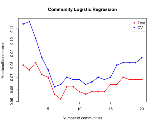
Figure 5: The 5-fold cross-validation errors (blue) and the test errors (red) of CLR on the spam data.

5 Conclusions

In this paper we have proposed sparse quadratic discriminant analysis, a classifier ranging between QDA and naive Bayes through a path of sparse graphical models. By allowing interaction terms into the model, this classifier relaxes the strict and often unreasonable assumption of naive Bayes. Moreover, the resulting estimates of interactions are sparse and easier to interpret compared to other existing classifiers that regularize QDA.

Motivated by the connection between the estimated precision matrices and single linkage clustering with the sample covariance matrices, we present the community Bayes model, a simple procedure applicable to non-Gaussian data and any likelihood-based classifiers. By exploiting the block-diagonal structure of the estimated correlation matrices, we reduce the problem into several sub-problems that can be solved independently. Simulated and real data examples show that the community Bayes model can improve accuracy and reduce variance in predictions.

A Proofs

A.1 Proof of Theorem 1

Proof.

The standard KKT conditions [2] of the optimization problem (5) give:

$$-n_{k}\left(\left(\hat{\mathbf{\Theta}}^{(k)}\right)^{-1}+\mathbf{S}^{(k)}\right)+\lambda\mathbf{\Gamma}^{(k)}=0,\mbox{ for }k=1,\ldots,K$$ (24)

where $\mathbf{\Gamma}^{(k)}$ is a $p\times p$ matrix with diagonal elements being zero:

$$\mathbf{\Gamma}^{(k)}=\left(\begin{array}[]{cccc}0&\gamma_{12}^{(k)}&\cdots&\gamma_{1p}^{(k)}\\ \gamma_{21}^{(k)}&0&\cdots&\gamma_{2p}^{(k)}\\ \vdots&\vdots&\ddots&\vdots\\ \gamma_{p1}^{(k)}&\gamma_{p2}^{(k)}&\cdots&0\end{array}\right).$$

Denote $\gamma_{ij}=(\gamma_{ij}^{(1)},\dots,\gamma_{ij}^{(K)})$ and $\hat{\theta}_{ij}=(\hat{\theta}_{ij}^{(1)},\ldots,\hat{\theta}_{ij}^{(K)})$. The subgradient $\gamma_{ij}\in\partial||\hat{\theta}_{ij}||_{2}$ for $i\neq j$, and

$$\partial||\theta_{ij}||_{2}=\begin{cases}B_{2}(1)&\mbox{if }\theta_{ij}=0;\\ \frac{\theta_{ij}}{||\theta_{ij}||_{2}}&\mbox{otherwise.}\end{cases}$$

Let $\hat{\mathbf{W}}^{(k)}=\left(\hat{\mathbf{\Theta}}^{(k)}\right)^{-1}.$ Then

$$\left(n_{1}(\hat{\mathbf{W}}_{ij}^{(1)}-\mathbf{S}_{ij}^{(1)}),\ldots,n_{K}(\hat{\mathbf{W}}_{ij}^{(K)}-\mathbf{S}_{ij}^{(K)})\right) = \lambda\frac{\hat{\theta}_{ij}}{||\hat{\theta}_{ij}||_{2}},\ \mbox{if }i\neq j\mbox{ and }\hat{\theta}_{ij}\neq 0;$$ (25)

$$\left\lVert\left(n_{1}(\hat{\mathbf{W}}_{ij}^{(1)}-\mathbf{S}_{ij}^{(1)}),\ldots,n_{K}(\hat{\mathbf{W}}_{ij}^{(K)}-\mathbf{S}_{ij}^{(K)})\right)\right\rVert_{2} \leq \lambda,\ \mbox{if }i\neq j\mbox{ and }\hat{\theta}_{ij}=0;$$ (26)

$$\left(\hat{\mathbf{W}}_{ii}^{(1)},\ldots,\hat{\mathbf{W}}_{ii}^{(K)}\right) = \left(\mathbf{S}_{ii}^{(1)},\ldots,\mathbf{S}_{ii}^{(K)}\right).$$ (27)

There exists an ordering of the vertices $\{1,\ldots,p\}$ such that the edge-matrix of the thresholded covariance graph is block-diagonal. For notational convenience, we will assume that the matrix is already in this order:

$$\mathbf{E}^{(\lambda)}=\left(\begin{array}[]{ccc}\mathbf{E}_{1}^{(\lambda)}&\cdots&0\\ \vdots&\ddots&\vdots\\ 0&\cdots&\mathbf{E}_{k(\lambda)}^{(\lambda)}\end{array}\right),$$ (28)

where $\mathbf{E}_{l}^{(\lambda)}$ represents the block of indices given by $\mathcal{V}_{l}^{(\lambda)},l=1,\ldots,k(\lambda)$.

We will construct $\hat{\mathbf{W}}^{(1)},\ldots,\hat{\mathbf{W}}^{(K)}$ having the same structure as $\mathbf{E}^{(\lambda)}$ which is a solution to the optimization problem (5). Note that if $\hat{\mathbf{W}}^{(k)}$ is block diagonal then so is its inverse. Let $\hat{\mathbf{W}}^{(k)}$ and its inverse $\hat{\mathbf{\Theta}}^{(k)}$ be given by:

$$\hat{\mathbf{W}}{}^{(k)}=\left(\begin{array}[]{ccc}\hat{\mathbf{W}}_{1}^{(k)}&\cdots&0\\ \vdots&\ddots&\vdots\\ 0&\cdots&\hat{\mathbf{W}}_{k(\lambda)}^{(k)}\end{array}\right),\ \hat{\mathbf{\Theta}}^{(k)}=\left(\begin{array}[]{ccc}\hat{\mathbf{\Theta}}_{1}^{(k)}&\cdots&0\\ \vdots&\ddots&\vdots\\ 0&\cdots&\hat{\mathbf{\Theta}}_{k(\lambda)}^{(k)}\end{array}\right),\mbox{ for all }k.$$ (29)

Define $\hat{\mathbf{W}}_{l}^{(k)}$ or equivalently $\hat{\mathbf{\Theta}}_{l}^{(k)}=\left(\hat{\mathbf{W}}_{l}^{(k)}\right)^{-1}$ via the following sub-problems

$$\hat{\mathbf{\Theta}}_{l}=\mbox{argmin}_{\mathbf{\Theta}_{l}^{(k)}\succ 0}\left\{-\sum_{k=1}^{K}n_{k}\left(\mbox{logdet }\mathbf{\Theta}_{l}^{(k)}-\mbox{tr}(\mathbf{S}_{l}^{(k)}\mathbf{\Theta}_{l}^{(k)})\right)+\lambda\sum_{\begin{subarray}{c}i,j\in\mathcal{V}_{l}^{(\lambda)}\\ i\neq j\end{subarray}}\|\theta_{ij}\|_{2}\right\}$$ (30)

for $l=1,\ldots,k(\lambda)$, where $\hat{\mathbf{\Theta}}_{l}=(\hat{\mathbf{\Theta}}_{l}^{(1)},\ldots,\hat{\mathbf{\Theta}}_{l}^{(K)})$, and $\mathbf{S}_{l}^{(k)}$ is a sub-block of $\mathbf{S}^{(k)}$ with row/column indices from $\mathcal{V}_{l}^{(\lambda)}\times\mathcal{V}_{l}^{(\lambda)}$. Thus for every $l$, $(\hat{\mathbf{\Theta}}_{l}^{(1)},\ldots,\hat{\mathbf{\Theta}}_{l}^{(K)})$ satisfies the KKT conditions corresponding to the $l^{\mbox{th}}$ block of the $p\times p$ dimensional problem.

By construction of the thresholded sample covariance graph, if $i\in\mathcal{V}_{l}^{(\lambda)}$and $j\in\mathcal{V}_{l^{\prime}}^{(\lambda)}$ with $l\neq l^{\prime}$, then $\tilde{\mathbf{S}}_{ij}\leq\lambda$. Hence, the choice $\hat{\mathbf{\Theta}}_{ij}^{(k)}=\hat{\mathbf{W}}_{ij}^{(k)}=0,\ k=1,\ldots,K$ satisfies the KKT conditions (26) for all the off-diagonal entries in the block-matrix (29). Hence $(\hat{\mathbf{\Theta}}^{(1)},\ldots,\hat{\mathbf{\Theta}}^{(K)})$ solves the optimization problem (5). This shows that the vertex-partition $\{\hat{\mathcal{V}}_{l}^{(\lambda)}\}_{1\leq l\leq\kappa(\lambda)}$ obtained from the estimated precision graph is a finer resolution of that obtained from the thresholded covariance graph, i.e., for every $l\in\{1,\ldots,k(\lambda)\}$, there is a $l^{\prime}\in\{1,\ldots,\kappa(\lambda)\}$ such that $\hat{\mathcal{V}}_{l^{\prime}}^{(\lambda)}\subset\mathcal{V}_{l}^{(\lambda)}$. In particular $k(\lambda)\leq\kappa(\lambda)$.

Conversely, if $(\hat{\mathbf{\Theta}}^{(1)},\ldots,\hat{\mathbf{\Theta}}^{(K)})$ admits the decomposition as in the statement of the theorem, then it follows from (26) that: for $i\in\hat{\mathcal{V}}_{l}^{(\lambda)}$and $j\in\mathcal{\hat{V}}_{l^{\prime}}^{(\lambda)}$ with $l\neq l^{\prime}$, we have $||\tilde{\mathbf{S}}_{ij}||_{2}\leq\lambda$ since $\hat{\mathbf{W}}_{ij}^{(k)}=0$ for $k=1,\ldots,K$. Thus the vertex-partition induced by the connected components of the thresholded covariance graph is a finer resolution of that induced by the connected components of the estimated precision graph. In particular this implies that $k(\lambda)\geq\kappa(\lambda)$.

Combining the above two we conclude $k(\lambda)=\kappa(\lambda)$ and also the equality (12). Since the labeling of the connected components is not unique, there is a permutation $\pi$ in the theorem.

Note that the connected components of the thresholded sample covariance graph $\mbox{G}^{(\lambda)}$ are nested within the connected components of $\mbox{G}^{(\lambda^{\prime})}$. In particular, the vertex-partition of the thresholded sample covariance graph at $\lambda$ is also nested within that of the thresholded sample covariance graph at $\lambda^{\prime}$. We have already proved that the vertex-partition induced by the connected components of the estimated precision graph and the thresholded sample covariance graph are equal. Using this result, we conclude that the vertex-partition induced by the components of the estimated precision graph at $\lambda$, given by $\{\hat{\mathcal{V}}_{l}^{(\lambda)}\}_{1\leq l\leq\kappa(\lambda)}$ is contained inside the vertex-partition induced by the components of the estimated precision graph at $\lambda^{\prime}$, given by $\{\hat{\mathcal{V}}_{l}^{(\lambda^{\prime})}\}_{1\leq l\leq\kappa(\lambda^{\prime})}$. ∎

A.2 Proof of Theorem 2

Proof.

Let $a=\min_{i,j\in\mathcal{V}_{l};l=1,\ldots,L}\tilde{\mathbf{R}}_{ij}^{0}$. First note that $\{\max_{ij}\left|\tilde{\mathbf{R}}_{ij}-\tilde{\mathbf{R}}_{ij}^{0}\right|<\frac{a}{2}\}\Rightarrow\{\hat{\mathcal{V}}_{l}=\mathcal{V}_{l},\forall l\}$ [22]. Then

$$P\left(\exists l,\hat{\mathcal{V}}_{l}\neq\mathcal{V}_{l}\right) \leq P\left(\max_{ij}\left|\tilde{\mathbf{R}}_{ij}-\tilde{\mathbf{R}}_{ij}^{0}\right|\geq\frac{a}{2}\right)$$

$$\leq P\left(\sum_{k=1}^{K}\max_{ij}n_{k}\left||\hat{\mathbf{R}}_{ij}^{(k)}|-|\mathbf{R}_{ij}^{(k)}|\right|\geq\frac{a}{2}\right)$$

$$\leq \sum_{k=1}^{K}P\left(\max_{ij}n_{k}\left||\hat{\mathbf{R}}_{ij}^{(k)}|-|\mathbf{R}_{ij}^{(k)}|\right|\geq\frac{a}{2K}\right)$$

$$\leq \sum_{k=1}^{K}P\left(\max_{ij}\left|\hat{\mathbf{R}}_{ij}^{(k)}-\mathbf{R}_{ij}^{(k)}\right|\geq\frac{a}{2n_{k}K}\right)$$

The second inequality is because $\left|\sqrt{a_{1}^{2}+\ldots+a_{m}^{2}}-\sqrt{b_{1}^{2}+\ldots+b_{m}^{2}}\right|\leq\left|a_{1}-b_{1}\right|+\ldots+\left|a_{m}-b_{m}\right|$.

Since $a\geq 16\pi K\sqrt{n_{k}\log p},$ we have $P(\max_{ij}\left|\hat{\mathbf{R}}_{ij}^{(k)}-\mathbf{R}_{ij}^{(k)}\right|\geq\frac{a}{2n_{k}K})\leq\frac{1}{p^{2}}$ by Theorem 4.1 of [14]. Therefore $P(\exists l,\hat{\mathcal{V}}_{l}\neq\mathcal{V}_{l})\leq\frac{K}{p^{2}}$.∎

References

- [1] Peter J Bickel and Elizaveta Levina. Some theory for fisher’s linear discriminant function,’naive bayes’, and some alternatives when there are many more variables than observations. Bernoulli, pages 989–1010, 2004.
- [2] Stephen Boyd and Lieven Vandenberghe. Convex optimization. Cambridge university press, 2009.
- [3] Peter Bühlmann, Philipp Rütimann, Sara van de Geer, and Cun-Hui Zhang. Correlated variables in regression: clustering and sparse estimation. Journal of Statistical Planning and Inference, 143(11):1835–1858, 2013.
- [4] Line Clemmensen, Trevor Hastie, Daniela Witten, and Bjarne Ersbøll. Sparse discriminant analysis. Technometrics, 53(4), 2011.
- [5] Patrick Danaher, Pei Wang, and Daniela M Witten. The joint graphical lasso for inverse covariance estimation across multiple classes. Journal of the Royal Statistical Society: Series B (Statistical Methodology), 2013.
- [6] Sandrine Dudoit, Jane Fridlyand, and Terence P Speed. Comparison of discrimination methods for the classification of tumors using gene expression data. Journal of the American statistical association, 97(457):77–87, 2002.
- [7] Jerome H Friedman. Regularized discriminant analysis. Journal of the American statistical association, 84(405):165–175, 1989.
- [8] Yaqian Guo, Trevor Hastie, and Robert Tibshirani. Regularized linear discriminant analysis and its application in microarrays. Biostatistics, 8(1):86–100, 2007.
- [9] Trevor Hastie, Andreas Buja, and Robert Tibshirani. Penalized discriminant analysis. The Annals of Statistics, pages 73–102, 1995.
- [10] Nadine Hussami and Robert Tibshirani. A component lasso. arXiv preprint arXiv:1311.4472, 2013.
- [11] WJ Krzanowski, Philip Jonathan, WV McCarthy, and MR Thomas. Discriminant analysis with singular covariance matrices: methods and applications to spectroscopic data. Applied statistics, pages 101–115, 1995.
- [12] B Boser Le Cun, John S Denker, D Henderson, Richard E Howard, W Hubbard, and Lawrence D Jackel. Handwritten digit recognition with a back-propagation network. In Advances in neural information processing systems. Citeseer, 1990.
- [13] Quefeng Li and Jun Shao. Sparse quadratic discriminant analysis for high dimensional data. Statist. Sinica, 2013.
- [14] Han Liu, Fang Han, Ming Yuan, John Lafferty, and Larry Wasserman. The nonparanormal skeptic. arXiv preprint arXiv:1206.6488, 2012.
- [15] Han Liu, John Lafferty, and Larry Wasserman. The nonparanormal: Semiparametric estimation of high dimensional undirected graphs. The Journal of Machine Learning Research, 10:2295–2328, 2009.
- [16] Rahul Mazumder and Trevor Hastie. Exact covariance thresholding into connected components for large-scale graphical lasso. The Journal of Machine Learning Research, 13:781–794, 2012.
- [17] Finbarr O’Sullivan. A statistical perspective on ill-posed inverse problems. Statistical science, pages 502–518, 1986.
- [18] Mee Young Park, Trevor Hastie, and Robert Tibshirani. Averaged gene expressions for regression. Biostatistics, 8(2):212–227, 2007.
- [19] Bradley S Price, Charles J Geyer, and Adam J Rothman. Ridge fusion in statistical learning. arXiv preprint arXiv:1310.3892, 2013.
- [20] Anthony John Robinson. Dynamic error propagation networks. PhD thesis, University of Cambridge, 1989.
- [21] Jiehuan Sun and Hongyu Zhao. The application of sparse estimation of covariance matrix to quadratic discriminant analysis. BMC bioinformatics, 16(1):48, 2015.
- [22] Kean Ming Tan, Daniela Witten, and Ali Shojaie. The cluster graphical lasso for improved estimation of gaussian graphical models. arXiv preprint arXiv:1307.5339, 2013.
- [23] Robert Tibshirani, Trevor Hastie, Balasubramanian Narasimhan, and Gilbert Chu. Diagnosis of multiple cancer types by shrunken centroids of gene expression. Proceedings of the National Academy of Sciences, 99(10):6567–6572, 2002.
- [24] DM Titterington. Common structure of smoothing techniques in statistics. International Statistical Review/Revue Internationale de Statistique, pages 141–170, 1985.
- [25] Daniela M Witten, Jerome H Friedman, and Noah Simon. New insights and faster computations for the graphical lasso. Journal of Computational and Graphical Statistics, 20(4):892–900, 2011.
- [26] Ping Xu, Guy N Brock, and Rudolph S Parrish. Modified linear discriminant analysis approaches for classification of high-dimensional microarray data. Computational Statistics & Data Analysis, 53(5):1674–1687, 2009.
- [27] Ming Yuan and Yi Lin. Model selection and estimation in regression with grouped variables. Journal of the Royal Statistical Society: Series B (Statistical Methodology), 68(1):49–67, 2006.
- [28] Hui Zou and Trevor Hastie. Regularization and variable selection via the elastic net. Journal of the Royal Statistical Society: Series B (Statistical Methodology), 67(2):301–320, 2005.