Block renormalization study on the nonequilibrium chiral Ising model

Abstract

We present a numerical study on the ordering dynamics of a one-dimensional nonequilibrium Ising spin system with chirality. This system is characterized by a direction-dependent spin update rule. Pairs of $+-$ spins can flip to $++$ or $--$ with probability $(1-u)$ or to $-+$ with probability $u$ while $-+$ pairs are frozen. The system was found to evolve into the ferromagnetic ordered state at any $u<1$ exhibiting the power-law scaling of the characteristic length scale $\xi\sim t^{1/z}$ and the domain wall density $\rho\sim t^{-\delta}$. The scaling exponents $z$ and $\delta$ were found to vary continuously with the parameter $u$. In order to establish the anomalous power-law scaling firmly, we perform the block spin renormalization analysis proposed by Basu and Hinrichsen [U. Basu and H. Hinrichsen, J. Stat. Mech. (2011) P11023]. Domain walls of $b$ sites are coarse-grained into a block spin $\sigma^{b}$, and the relative frequencies of two-block patterns $\sigma^{b}_{1}\sigma^{b}_{2}$ are measured in the $b\to\infty$ and $t\to\infty$ limit. These indices are expected to be universal. By performing extensive Monte Carlo simulations, we find that the indices also vary continuously with $u$ and that their values are consistent with the scaling exponents found in the previous study. This study serves as another evidence for the claim that the nonequilibrium chiral Ising model displays the power-law scaling behavior with continuously varying exponents.

I Introduction

Macroscopic systems display an intriguing dynamic scaling behavior upon ordering Glauber (1963); Bray (2001). When a system in an ordered phase is quenched from a disordered configuration, the characteristic size $\xi$ of ordered domains increases with time and microscopic details become less and less important. Consequently, there emerges a dynamic scaling behavior that is classified into a universality class depending on symmetry, conservation, and so on.

Each universality class is characterized by the power-law scaling of the length scale $\xi\sim t^{1/z}$ with a universal dynamic exponent $z$. For example, equilibrium systems with a scalar order parameter, such as the Ising model, have $z=2$ under the nonconserved dynamics and $z=3$ under the conserved dynamics in the ordered phase Newman et al. (1990); Bray and Rutenberg (1994). Systems with a vector order parameter also have distinct values of $z$ depending on the presence of the conservation law Newman et al. (1990); Bray and Rutenberg (1994).

Recently, the ordering dynamics in a nonequilibrium chiral Ising model (NCIM) was studied numerically in one dimension Kim et al. (2013). The NCIM, which will be explained in detail in Sec. II, has two important features. It has the ferromagnetic states with all spins up or down as the two equivalent absorbing states. Namely, once the system reaches one of the two ferromagnetic states, it stays there forever. In addition, the NCIM has a direction-dependent spin update rule, which makes the system chiral. The chirality breaks the spin up-down symmetry.

The model without chirality is equivalent to the nonequilibrium kinetic Ising model, whose ordering dynamics is described by $z=2$ Mussawisade et al. (1998); Menyhárd and Ódor (2000). When the chirality turns on, the dynamic exponent and the other exponents are found to vary continuously as a function of a model parameter Kim et al. (2013). Such a phenomenon is very rare with only a few examples Lee and Privman (1997); Jain (2005). It might be attributed to the different symmetry property of the NCIM. However, its origin is not revealed yet. The current status urges us to establish the universality class firmly by an independent means.

Basu and Hinrichsen proposed a numerical method to identify a dynamic universality class by using a block spin transformation Basu and Hinrichsen (2011). Adopting the idea of the real-space renormalization group transformation Maris and Kadanoff (1978); Kadanoff (2000), one divides a one dimensional lattice of $L$ sites into $L/b$ blocks of size $b$ and coarse-grains a spin configuration $\{\sigma_{n}|n=1,\cdots,L\}$ with a block-spin configuration $\{\sigma^{b}_{n}|n=1,\cdots,L/b\}$. Then, for any pattern $c=(xy\cdots)$, one can define a correlation function

$$P_{c}(b,t)=\left\langle\delta(\sigma^{b}_{n}(t),x)\delta(\sigma^{b}_{n+1}(t),y)\cdots\right\rangle\ ,$$ (1)

where $\delta(x,y)$ is the Kronecker delta, $\sigma^{b}_{n}(t)$ denotes the block spin at site $n$ at time $t$, and $\left\langle\cdot\right\rangle$ denotes the average over ensembles as well as $n$. The ratios between the correlation functions of different patterns turn out to converge to universal values in the $t\to\infty$ limit followed by the $b\to\infty$ limit. This universal feature was tested for some dynamic universality classes Basu and Hinrichsen (2011).

We apply the block spin analysis to the NCIM in order to confirm that the NCIM is characterized by the continuously-varying critical exponents. In Sec. II, we introduce the NCIM and give a brief review of the numerical result in Ref. Kim et al. (2013). Section III presents the main result of the block spin analysis for the NCIM. This result is fully consistent with the previous numerical result and strengthens the claim of the universality class with the continuously-varying critical exponents. The ratio of the correlation functions in Eq. (1) is related to the critical exponent through a scaling relation. The scaling relation was proposed in Ref. Basu and Hinrichsen (2011) on the ground of the scaling ansatz. We present a microscopic theory for the scaling relation in Sec. IV. We summarize this work with discussions in Sec. V.

II Nonequilibrium chiral Ising model

To study a coarsening dynamics of a one dimensional Ising spin chain $\{s_{n}=\pm|n=1,\cdots,L\}$ with chirality, the authors have suggested the NCIM with the following dynamic rules Kim et al. (2013),

$$+-\stackrel{{\scriptstyle u}}{{\longrightarrow}}-+ ,\quad -+\stackrel{{\scriptstyle\bar{u}}}{{\longrightarrow}}+-,$$

$$+-\stackrel{{\scriptstyle v/2}}{{\longrightarrow}}\begin{cases}++\\ --\end{cases} ,\quad -+\stackrel{{\scriptstyle\bar{v}/2}}{{\longrightarrow}}\begin{cases}++\\ --\end{cases},$$ (2)

where $u~{}(\bar{u})$ and $v~{}(\bar{v})$ are the transition rates for the spin exchange and the single spin flip dynamics of the local configuration $+-$ ($-+$), respectively. We have assumed periodic boundary conditions. The chirality can be incorporated into the model by taking different transition rates for $+-$ and $-+$ domain walls. The NCIM has two equivalent ferromagnetically ordered states with all spins up or down. These states are absorbing in the sense that the system cannot get out of the states by the above dynamic rules.

In addition to its own merit as a minimal model for the chiral dynamics, the NCIM can be applied to a flocking phenomenon of active Brownian particles by regarding the Ising spin states $+$ and $-$ as the directions of motion of particles in one dimension. The flocking model using the active spins is found in Ref. Solon and Tailleur (2013).

The chirality breaks the spin up-down symmetry of the Ising model. Unlike the magnetic field which favors one of the spin states, the chirality does not prefer any of the spin states. In fact, the NCIM is symmetric under the simultaneous inversion of spin and space, $s_{n}\to-s_{L-n+1}$. In higher dimensions, this chirality turned out to be irrelevant for Ising-like spin models with order-disorder transitions Bassler and Schmittmann (1994) (see also Ref. Dutta and Park (2011) for a generalization to $N$-vector models, which showed that chirality is relevant for $N\geq 2$). However the one dimensional system with chirality seems to exhibit intriguing scaling behaviors with continuously varying exponents Kim et al. (2013).

It is convenient to map the Ising spin system to a reaction diffusion system of two species $A$ and $B$ by introducing a random variable $\sigma_{n}\in\{A,B,O\}$: A site $n$ is regarded as being occupied by an $A$ particle [$\sigma_{n}=A$] if $(s_{n}s_{n+1})=(+-)$. It is regarded as being occupied by a $B$ particle [$\sigma_{n}=B$] if $(s_{n}s_{n+1})=(-+)$. Otherwise, it is regarded as being empty [$\sigma_{n}=O$]. Within this scheme, all sites are empty in the absorbing states. Due to the correspondence with Ising spin configurations, the two species should be alternating in space and the number of $A$ particles should be the same as that of $B$ particles. Under the symmetry operation $s_{n}\to-s_{L-n+1}$, a particle configuration is mapped to the mirror image with the particle species being invariant.

The spin dynamic rules are translated as follows. With rate $v$ species $A$ hops to one of its nearest neighbors chosen with equal probability, and with rate $u$ species $A$ branches two $A$’s at both nearest neighbor sites and it changes to another species ($A\to ABA$). The dynamics of species $B$ is the same as above with rates given by the barred parameters. Whenever two species happen to occupy the same site by either hopping or branching event, both particles annihilate immediately ($A+B\to O$).

Time evolution of the NCIM with $\bar{u}=\bar{v}=0$ is illustrated in terms of the spin variable $\{s_{n}\}$ in Fig. 1(a) and in terms of the particle variable $\{\sigma_{n}\}$ in Fig. 1(b). The chirality gives rise to an interesting space-time pattern. The motions of $A$ and $B$ species are asymmetric, while none of the spin states are preferred. As the dynamics proceeds, a characteristic domain size increases and the density of particles decreases with time. The ordering or coarsening dynamics is characterized by the power-law scaling of the characteristic domain size

$$\xi(t)\sim t^{1/z}\ ,$$ (3)

and the domain wall or particle density

$$\rho(t)\sim t^{-\delta},$$ (4)

with the dynamic exponent $z$ and the density decay exponent $\delta$.

Figure 1: (Color online) Space-time patterns of the Ising spins with chirality ($\bar{u}=\bar{v}=0$ and $u=1-v=0.5$) in (a) and (b), and without chirality ($u=v=\bar{u}=\bar{v}=0.5$) in (c) and (d). Spin dynamics are shown in (a) and (c), where black (white) pixels represent sites of $+~{}(-)$ states. Particle dynamics are shown in (b) and (d), where red (blue) pixels represent $A~{}(B)$ particle. The horizontal and vertical directions correspond to the spatial and temporal directions, respectively.

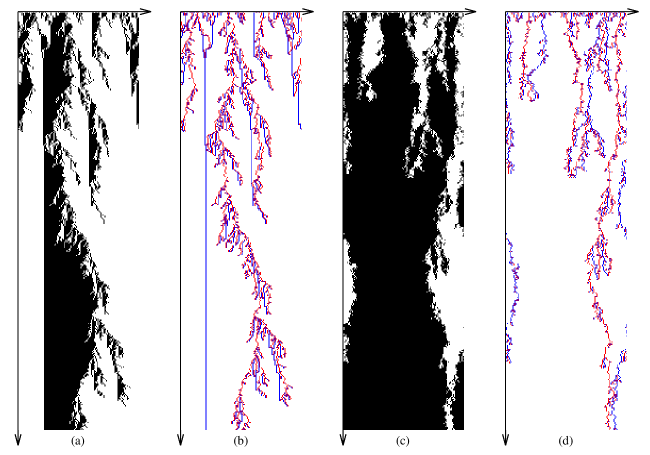
Without chirality ($u=\bar{u}$ and $v=\bar{v}$), the NCIM reduces to the nonequilibrium kinetic Ising model (NKIM) or the reaction diffusion system Mussawisade et al. (1998); Menyhárd and Ódor (2000); ben Avraham et al. (1994); Takayasu and Tretyakov (1992) (see Figs. 1(c) and(d)) which is exactly solvable ben Avraham et al. (1994). The exact solution reveals that the ordering dynamics belongs to the universality class of the model at $u=\bar{u}=0$. It corresponds to the Ising model under the zero-temperature Glauber dynamics Glauber (1963), or equivalently the voter model Cox (1989); Liggett (1995). The critical exponents are $z=2$ and $\delta=1/2$.

When the chirality sets in ($u\neq\bar{u}$ or $v\neq\bar{v}$), the model is not solvable any more. The model has been studied in various regions of the parameter space. For example, when $v=\bar{v}$ and $u\neq\bar{u}$, it becomes the mixture of the asymmetric simple exclusion process and the voter model studied in Ref. Belitscky et al. (2001); MacPhee et al. (2010). The ordering dynamics of the NCIM has been studied numerically in Ref. Kim et al. (2013). Surprisingly, the numerical study reveals that the dynamic exponent and the density decay exponent vary continuously within the range $1<z\leq 2$ and $0<\delta\leq 1/2$. We will provide an independent evidence for the continuously varying critical exponents in the following sections.

III Block spin analysis

At criticality, the scaling functions as well as the critical exponents are universal. Extending this idea, Basu and Hinrichsen Basu and Hinrichsen (2011) proposed that the spatial correlation of spins in the long time and large distance limit can be used in identifying a dynamic universality class. This is accomplished by coarse-graining a ‘spin’ configuration with that of a ‘block spin’. As in the real-space renormalization group transformation Maris and Kadanoff (1978); Kadanoff (2000), $b$ spins in a row are coarse-grained by a single block spin. Then, large-distance correlations are measured in terms of the block spins in the $b\to\infty$ limit.

We apply the coarse graining scheme to the particle or domain wall variable $\sigma_{n}\in\{A,B,O\}$ of the NCIM. The coarse-graining should preserve the symmetry and the conservation of the system. It should also preserve the absorbing nature of the vacuum state. The following coarse-graining scheme fulfills the requirements.

To a given block of size $b$, the number of $A$ and $B$ particles are denoted by $N(A)$ and $N(B)$, respectively. If $N(A)=N(B)=0$, the block is in a vacuum state and it is assigned to a state ${O}$. If $N(A)>N(B)$, the block separates the $+$ domain in the left from the $-$ domain in the right. Thus it is assigned to a state $A$. If $N(A)<N(B)$, the block separates the $-$ domain in the left from the $+$ domain in the right, so it is assigned to a state $B$. If $N(A)=N(B)\neq 0$, the block is not in the vacuum state, nor does it separate different domains. Hence we need to assign a block state different from $A$, $B$, and $O$. Furthermore, due to the chirality, we need to assign a different block state depending on whether the domain walls have an $AB$ ordering or $BA$ ordering. We will assign a block state $X$ for the former case and $Y$ for the latter. The coarse-graining rule is summarized below:

$$\sigma^{b}=\begin{cases}{O}&\mbox{if }N(A)=N(B)=0\\ {A}&\mbox{if }N(A)>N(B)\\ {B}&\mbox{if }N(A)<N(B)\\ {X}&\mbox{if }N(A)=N(B)\neq 0\mbox{ and $AB$ ordering}\\ {Y}&\mbox{if }N(A)=N(B)\neq 0\mbox{ and $BA$ ordering}\end{cases}\ .$$ (5)

Note that the block spin $\sigma^{b}$ takes on five different states. This is in contrast to the Ising system without chirality where one needs only three different block states Basu and Hinrichsen (2011). Due to the chirality, ${A}$ and ${B}$ should be distinguished, so should ${X}$ and ${Y}$. Under the symmetry operation $s_{n}\to-s_{L-n+1}$, ${A}$ and ${B}$ remain the same while ${X}$ is transformed to ${Y}$ and vice versa.

Using the coarse-graining rule, we evaluate numerically the correlation function $P_{c}(b)$ defined in Eq. (1) especially for all two-blocks patterns

$$\begin{split}c\in&\{{OO},{OA},{AO},{OB},{BO},{AB},{BA},{XO},{OX}\\ &{YO},{OY},{XA},{BX},{AY},{YB},{XX},{YY}\}.\end{split}$$ (6)

Patterns ${AA}$, ${BB}$, ${XB}$, ${AX}$, ${BY}$, ${YA}$, ${XY}$, and ${YX}$ are forbidden by the background spin dynamics. We concentrate on the model with $\bar{u}=\bar{v}=0$ and $u+v=1$, which was referred to as the maximum chiral model (MCM) in Ref. Kim et al. (2013). In this model, $A$ particles branch with the probability $u$ and hops with the probability $v=1-u$ while $B$ particles are frozen except when the instantaneous pair annihilation ($A+B\to O$) occurs.

Monte Carlo simulations are performed in systems of sizes $L=2^{24}$ at $u=0.0$ and $0.1$, $L=2^{23}$ at $u=0.2$ and $0.3$, $L=2^{22}$ at $u=0.4$, $0.5$, and $0.6$, $L=2^{21}$ at $u=0.7$, $0.8$, and $0.9$, and $L=2^{20}$ at $u=1.0$. The initial configuration is taken to be the fully occupied state $(\cdots ABAB\cdots)$ that is equivalent to the antiferromagnetic state $(\cdots+-+-\cdots)$. During simulation, the correlation functions $P_{c}(b,t)$ are evaluated for all two-blocks patterns $c$ in Eq. (6) at times $t=2^{l}$ with $l\leq 24$. The block sizes are $b=2^{k}$ with $k\leq 5$. All the data are obtained by averaging over $N_{S}\leq 5000$ independent samples.

Figure 2: Temporal decay of the two-blocks correlation function $P_{c}(b=4)$ at the model parameter $u=0.3$. Also shown is the overall particle density $\rho(t)$.

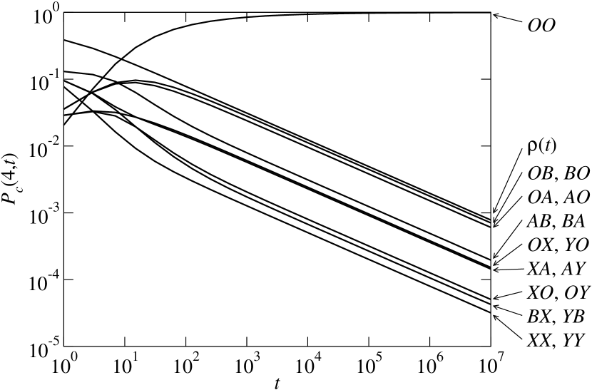
Figure 2 presents the two-blocks correlation functions with $b=4$ in the MCM with $u=0.3$. After a transient period, all the correlation functions except for the pattern $c={OO}$ decay algebraically with the density decay exponent $\delta$. Since the system eventually orders, $P_{{OO}}$ converges to $1$ in the $t\to\infty$ limit. This temporal scaling is also observed for other values of $b$:

$$P_{c}(b,t)\sim t^{-\delta}\quad\text{for}\quad c\neq{OO}\ .$$ (7)

Note that the correlation functions are not independent of each other. The symmetry under $s_{n}\to-s_{L-n+1}$ requires that

$$\begin{split}P_{{OA}}=P_{{AO}},\quad P_{{OB}}=P_{{BO}},\\ P_{{AB}}=P_{{BA}},\quad P_{{XO}}=P_{{OY}},\\ P_{{OX}}=P_{{YO}},\quad P_{{XX}}=P_{{YY}},\\ P_{{XA}}=P_{{AY}},\quad P_{{BX}}=P_{{YB}}.\end{split}$$ (8)

Following Ref. Basu and Hinrichsen (2011), we define

$$S_{c}(b,t)\equiv\frac{P_{c}(b,t)}{\sum_{c^{\prime}\neq{OO}}{P_{c^{\prime}}(b,t)}}=\frac{P_{c}(b,t)}{1-P_{{OO}}{(b,t)}}.$$ (9)

It measures the relative frequency of a block pattern $c$ among all patterns but the vacuum pattern ${OO}$. Upon taking the ratio, the temporal dependence cancels out and the amplitudes determine $S_{c}(b,t)$. The scale invariance suggests that the quantity should converge to a universal value Basu and Hinrichsen (2011)

$$S_{c}=\lim_{b\to\infty}S_{c}(b)$$ (10)

with

$$S_{c}(b)=\lim_{t\to\infty}S_{c}(b,t)\ .$$ (11)

Figure 3: (a) $S_{{OB}}(b,t)$ for $b=1,2,\ldots,32$ (from top to bottom) and (b) $S_{{OB}}(b)$ at the model parameter $u=0.3$.

Figure 3(a) presents the relative frequency $S_{{OB}}(b,t)$ of a pattern ${OB}$ at several levels of coarse graining at $u=0.3$. It converges to a constant value $S_{{OB}}(b)$ in the $t\to\infty$ limit. The extrapolated values are plotted as a function of $1/b$ in Fig. 3(b), from which we can estimate $S_{{OB}}$. In practice, we adopted a power-law fitting to the forms $S_{c}(b,t)=S_{c}(b)+at^{-\chi}$ and $S_{c}(b)=S_{c}+a^{\prime}b^{-\chi^{\prime}}$.

Figure 4: $S_{c}$ for two-blocks patterns $c$. Lines are a guide to an eye.

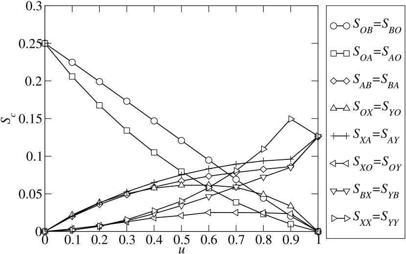
Repeating the same procedure, we obtain the relative frequency for all patterns. They are presented in Fig. 4. At $u=0$, $A$ particles diffuse without branching and annihilate in pairs with $B$ particles upon collision. Hence, when $t\gg b^{2}$, the block spin configurations consist of isolated ${A}$s and ${B}$s in the sea of ${O}$s. It explains the numerical result that $S_{{OB}}=S_{{BO}}=S_{{OA}}=S_{{AO}}=1/4$ with the others being zero. At $u=1$, the system reaches an active steady state with a finite particle density. Block spins are in a state of ${A}$, ${B}$, ${X}$, or ${Y}$ equally likely, and a spatial correlation is absent in the $b\to\infty$ limit. Thus, $S_{{AB}}=S_{{BA}}=S_{{XA}}=S_{{AY}}=S_{{BX}}=S_{{YB}}=S_{{XX}}=S_{{YY}}=1/8$ and all the others are zero.

As is noticeable in Fig. 4, $S_{c}$ seems discontinuous at $u=1$. The model at $u=1$ is a singular limit in the sense that there is no chance of falling into absorbing states once initial particle density is finite. Thus unlike the case of $u<1$, $P_{OO}(b,t)$ cannot approach 1 with $t$. We speculate that the sharp change of $S_{c}$’s near $u=1$ could be caused because $P_{OO}(b,\infty)$ changes abruptly at $u=1$.

As the model parameter $u$ varies, each value of $S_{c}$ varies continuously. Under the hypothesis that $S_{c}$ should be universal, Fig. 4 provides an evidence for the continuously varying critical exponents of the NCIM. In Sec. IV, we will estimate the critical exponent $z\delta$ using the values of $S_{c}$’s.

IV Critical exponent $z\delta$

For general one-dimensional models with absorbing states, one can introduce a random variable $\rho_{n}$ at each site $n$ ($n=1,2,\ldots,L$) which takes either 1 or 0. Conventionally, $\rho_{n}$ is defined in such a way that a configuration is absorbing if and only if $\rho_{n}=0$ for all $n$. In this section, however, we only assume that the condition $\rho_{n}=0$ for all $n$ is a necessary condition of system’s being in one of absorbing states. Still, however, the average of $\rho_{n}$ over space and ensemble

$$\rho(t)=\frac{1}{L}\sum_{n}\langle\rho_{n}\rangle$$ (12)

can play the role of an order parameter. For convenience, we will say that a site $n$ is occupied (vacant) if $\rho_{n}=1$ (0), even though $\rho_{n}=0$ does not necessarily imply that the site $n$ is truly devoid of any particles of the background dynamic model. If we limit ourselves to the stochastic behavior of $\rho_{n}$ instead of the domain wall variables $\sigma_{n}$, the block configurations become simpler than those in Sec. III. A block of size $b$ is assigned to be occupied only when it contains at least one occupied site. The specific choice of $\rho_{n}$ for the NCIM will be taken later.

Combining Eqs. (3) and (4), the density scales as

$$\rho\sim\xi^{-\alpha}$$ (13)

with the exponent

$$\alpha=z\delta.$$ (14)

Under the assumption of the scale invariance during the critical dynamics, it is claimed in Ref. Basu and Hinrichsen (2011) that

$$\lim_{b\to\infty}\lim_{t\to\infty}\frac{P_{1}(b,t)}{P_{1}(2b,t)}=2^{-\alpha},$$ (15)

where $P_{1}(b,t)$ is the probability that a block of size $b$ is occupied, that is, it contains at least one occupied site. Formally speaking, $P_{1}(b,t)$ is defined as

$$P_{1}(b,t)=\lim_{L\rightarrow\infty}\frac{1}{L}\sum_{n}\left\langle 1-V_{n,b}\right\rangle,$$ (16)

where $V_{n,b}\equiv\prod_{r=0}^{b-1}(1-\rho_{n+r})$ with $V_{n,0}\equiv 1$. Note that $(1-V_{n,b})$ can be interpreted as the ‘block spin’ in the sense of Ref. Basu and Hinrichsen (2011). We will provide a general microscopic theory for the condition under which the relation (15) is valid.

To analyze Eq. (15) systematically, we introduce three types of correlation functions such as

$$P_{\rho\rho}(r,t) =\frac{1}{L}\sum_{n}\left\langle\rho_{n}\rho_{n+r}\right\rangle,$$ (17)

$$P_{\rho v\rho}(r,t) =\frac{1}{L}\sum_{n}\left\langle\rho_{n}V_{n+1,r-1}\rho_{n+r}\right\rangle,$$ (18)

$$P_{v\rho}(r,t) =\frac{1}{L}\sum_{n}\left\langle V_{n,r}\rho_{n+r}\right\rangle.$$ (19)

Taking the translational invariance for granted, $P_{\rho\rho}(r,t)$ is the joint probability that two sites separated by a distance $r$ are occupied simultaneously. Similarly, $P_{\rho v\rho}(r,t)$ denotes the joint probability that two sites separated by a distance $r$ are occupied with all intermediate sites being vacant. $P_{v\rho}(r,t)$ is the joint probability that a site is occupied and preceded by $r$ empty sites. For example, $P_{\rho v\rho}(1,t)=\langle\bullet\bullet\rangle$, $P_{v\rho}(1,t)=\langle\circ\bullet\rangle$, $P_{\rho v\rho}(2,t)=\langle\bullet\circ\bullet\rangle$, $P_{v\rho}(2,t)=\langle\circ\circ\bullet\rangle$, and so on, where $\bullet$ ($\circ$) signifies an occupied (a vacant) site.

The first step is to represent $\rho(t)$ and $P_{1}(b,t)$ in terms of these correlation functions. The identity $V_{n,1}+\rho_{n}=1~{}(\circ+\bullet=1)$ yields that $\rho(t)=P_{v\rho}(1,t)+P_{\rho v\rho}(1,t)~{}(\langle\bullet\rangle=\langle\circ\bullet\rangle+\langle\bullet\bullet\rangle)$ and $P_{v\rho}(r-1,t)=P_{\rho v\rho}(r,t)+P_{v\rho}(r,t)~{}(\langle\circ\cdots\bullet\rangle=\langle\bullet\circ\cdots\bullet\rangle+\langle\circ\circ\cdots\bullet\rangle)$. Applying the second relation iteratively, we get, for any $1\leq b\leq L$,

$$\rho(t)=\sum_{r=1}^{b}P_{\rho v\rho}(r,t)+P_{v\rho}(b,t).$$ (20)

In the following discussion, $L\rightarrow\infty$ limit is assumed to be taken first. Note that under the thermodynamic limit $\rho(t)>0$ for finite $t$ once $\rho(t=0)>0$ and no sample can fall into one of absorbing states up to finite $t$.

Using the identity $V_{n,1}=1-\rho_{n}$ again, one can decompose $V_{n,b}=V_{n,b-1}V_{n+b-1,1}$ into $V_{n,b}=V_{n,b-1}-V_{n,b-1}\rho_{n+b-1}$. Hence, we obtain $P_{1}(b,t)=P_{1}(b-1,t)+P_{v\rho}(b-1,t)$. Applying the relation iteratively and using $P_{1}(1,t)=\rho(t)$, we can rewrite $P_{1}(b,t)$ as

$$P_{1}(b,t) =\rho(t)+\sum_{r=1}^{b-1}P_{v\rho}(r,t)$$

$$=\rho(t)+\sum_{r=1}^{b-1}\left(\rho(t)-\sum_{k=1}^{r}P_{\rho v\rho}(k,t)\right)$$

$$=b\rho(t)-\sum_{r=1}^{b}(b-r)P_{\rho v\rho}(r,t),$$ (21)

where the relation (20) is used in the second line. Consequently we obtain

$$R(b,t)\equiv\frac{P_{1}(b,t)}{P_{1}(2b,t)}=\frac{\displaystyle b-\sum_{r=1}^{b}(b-r)F(r,t)}{\displaystyle 2b-\sum_{r=1}^{2b}(2b-r)F(r,t)},$$ (22)

where

$$F(r,t)\equiv P_{\rho v\rho}(r,t)/\rho(t).$$ (23)

It can be interpreted as the conditional probability of $V_{n+1,r-1}\rho_{n+r}=1$ given that $\rho_{n}=1$. Namely, $F(r,t)$ is the probability that a given particle would find its first neighbor particle at distance $r$ and at time $t$.

From Eq. (20), we find a normalization condition

$$\sum_{r=1}^{b}F(r,t)+\frac{P_{v\rho}(b,t)}{\rho(t)}=1.$$ (24)

According to the probability interpretation of $F(r,t)$ above, we can claim that

$$\sum_{r=1}^{\infty}F(r,t)\equiv\lim_{b\to\infty}\sum_{r=1}^{b}F(r,t)=1,$$ (25)

which is equivalent to

$$\lim_{b\rightarrow\infty}\frac{P_{v\rho}(b,t)}{\rho(t)}=0$$ (26)

for any $t$. Since $\rho(t)$ is finite for finite $t$, Eq. (26) should be satisfied because the mean distance between two occupied sites should be $1/\rho(t)$. Recall that the thermodynamic limit is assumed to be taken already.

It is quite tempting to claim that

$$\lim_{b\rightarrow\infty}\lim_{t\rightarrow\infty}\frac{P_{v\rho}(b,t)}{\rho(t)}=0$$ (27)

and

$$\sum_{r=1}^{\infty}F_{\infty}(r)=1,$$ (28)

where $F_{\infty}(r)=\lim_{t\to\infty}F(r,t)$. Unfortunately, however, this is not always true. A counter example can be found from the pair annihilation model ($A+A\rightarrow 0$). In this example, we define $\rho_{n}$ such that $\rho_{n}=1$ if a particle is present at site $n$ and 0 otherwise. Since $\rho(t)\sim t^{-1/2}$ and $P_{\rho\rho}(r,t)\sim rt^{-3/2}$ Derrida and Zeitak (1996); Bares and Mobilia (1999); Park et al. (2001); Masser and ben Avraham (2001) we get

$$0\leq F(r,t)\leq P_{\rho\rho}(r,t)/\rho(t)\sim t^{-1},$$ (29)

where we have used $P_{\rho v\rho}(r,t)\leq P_{\rho\rho}(r,t)$. Thus, $F_{\infty}(r)=0$ for all $r$, which cannot be consistent with Eq. (28).

The normalization condition Eq. (28) for $F_{\infty}(r)$ is not satisfied when vacant sites form an infinite interval in the $t\to\infty$ limit. Therefore, we introduce a parameter $0\leq\phi\leq 1$ such that

$$\sum_{r=1}^{\infty}F_{\infty}(r)=1-\phi.$$ (30)

Then, the numerator of Eq. (22) can be written as

$$G(b) \equiv b-\sum_{r=1}^{b}(b-r)F_{\infty}(r)$$

$$=b\phi+b\sum_{r=b+1}^{\infty}F_{\infty}(r)+\sum_{r=1}^{b}rF_{\infty}(r).$$ (31)

Assuming the scale invariance, we expect $F_{\infty}(r)\sim r^{-\theta}$ with a critical exponent $\theta$ which should be larger than 1 by Eq. (30). Within this assumption, one can easily see that

$$b\sum_{r=b+1}^{\infty}F_{\infty}(r)\sim\sum_{r=1}^{b}rF_{\infty}(r)\sim b^{\min[0,2-\theta]}\ll b$$ (32)

for large $b$.

Suppose that $\phi$ is strictly positive. Then, $G(b)\simeq bc+O(b^{\min[0,2-\theta]})$ and

$$\lim_{t\to\infty}R(b,t)=2^{-1}\ ,$$ (33)

which gives $\alpha=1$. The pair annihilation model belongs to this category with $\phi=1$. Since the model is characterized with $z=2$ and $\delta=1/2$, the relation (15) appears to be valid. However, we believe that this coincidence is fortuitous. As a counter example, consider the two-species diffusion-limited annihilation model ($A+B\rightarrow 0$) and interpret $\rho_{n}$ as the particle occupation number irrespective of species. If the system evolves from a random initial condition, $\rho(t)\sim t^{-1/{2z}}$ with $z=2$ Toussaint and Wilczek (1983); Kang and Redner (1984); Branmson and Lebowitz (1988); Leyvraz and Redner (1992). Since inter-particle distances diverges as $1/\rho\sim t^{1/2z}$ and there is no branching event which can place a particle close to a given particle, $F_{\infty}(r)$ should be 0 for finite $r$. Thus, Eq. (15) leads to $\alpha=1$ that is different from $z\delta=1/2$. In other words, unlike the general idea of the renormalization group, Eq. (15) has limited applicability when the normalization in Eq. (28) fails.

If the normalization is valid ($\phi=0$) and $F_{\infty}(r)\sim r^{-\theta}$ for large $r$, the asymptotic behavior of $G(b)$ becomes

$$G(b)\sim\begin{cases}b^{2-\theta}&1<\theta<2,\\ \ln b&\theta=2,\\ \text{const}&\theta>2,\end{cases}$$ (34)

which results in

$$\lim_{b\rightarrow\infty}\lim_{t\to\infty}R(b,t)=\begin{cases}2^{-(2-\theta)},&1<\theta<2,\\ 1,&\theta\geq 2.\end{cases}$$ (35)

Assuming that Eq. (15) is valid with $\alpha=z\delta$ for any $\theta$, Eq. (35) suggests that $\alpha$ should be zero for $\theta\geq 2$. Since $z$ cannot be zero, $\delta$ should be zero if $\theta\geq 2$. That is, the system with $\theta\geq 2$ should be in the active phase and $F_{\infty}(t)$ should actually decay exponentially. Thus, the necessary conditions that a critical system satisfies Eq. (15) are Eq. (28) and $F_{\infty}(r)\sim r^{-\theta}$ with $1<\theta<2$ (or $\alpha<1$) for sufficiently large $r$.

Assuming that all necessary conditions are satisfied, we will now argue that $2-\theta$ is indeed equal to $\alpha$. We start from the observation that

$$\langle\rho_{i}\rho_{i+r}\rangle= P_{\rho v\rho}(r,t)+\sum_{k=1}^{r-1}\left\langle\rho_{i}V_{i+1,k-1}\rho_{i+k}\rho_{i+r}\right\rangle,$$ (36)

where we have exploited the translational invariance of the system. Employing a cluster mean field-type approximation such that

$$\left\langle\rho_{n}V_{i+1,k-1}\rho_{n+k}\rho_{n+r}\right\rangle\approx\frac{P_{\rho v\rho}(k,t)P_{\rho\rho}(r-k,t)}{\rho(t)},$$ (37)

we get

$$C_{\infty}(r)\approx F_{\infty}(r)+\sum_{k=1}^{r-1}F_{\infty}(k)C_{\infty}(r-k),$$ (38)

where $C_{\infty}(r)=\lim_{t\to\infty}P_{\rho\rho}(r,t)/\rho(t)$. Introducing generating functions

$$\widetilde{C}_{\infty}(s)=\sum_{r=1}^{\infty}e^{-sr}C_{\infty}(r),\quad\widetilde{F}_{\infty}(s)=\sum_{r=1}^{\infty}e^{-sr}F_{\infty}(r),$$ (39)

and using the convolution theorem, we get

$$\widetilde{C}_{\infty}(s)\approx\frac{\widetilde{F}_{\infty}(s)}{1-\widetilde{F}_{\infty}(s)}.$$ (40)

Figure 5: (Color online) Correlation functions $C(r,t)$ (blue) and $F(r,t)$ (red), and their product (black). The dot-dashed lines with indicated slopes are guides to the eyes. The data are obtained for the NCIM with the parameter values $u=1-v=0.3$ and $\bar{u}=\bar{v}=0$. The lattice size is $L=2^{20}$ and the simulation time is up to $t=2^{25}$. The data are averaged over more than 100 samples and log-binned.

From the scale invariance, we expect $C(r)\sim r^{-\alpha}$ and, in turn,

$$\widetilde{C}_{\infty}(s) =\sum_{r=1}C_{\infty}(r)e^{-sr}\approx\int_{1}^{\infty}r^{-\alpha}e^{-sr}dr$$

$$\sim s^{-(1-\alpha)}\int_{0}^{\infty}u^{-\alpha}e^{-u}du\sim s^{-(1-\alpha)},$$ (41)

which diverges as $s\rightarrow 0$ if $\alpha<1$ (recall that this is one of necessary conditions). Since $\widetilde{F}_{\infty}(s)\rightarrow 1$ as $s\rightarrow 0$ due to Eq. (28), $1-\widetilde{F}_{\infty}(s)$ should approach 0 as $s\to 0$ for Eq. (40) to be valid. For small $s$, we obtain

$$1-\widetilde{F}_{\infty}(s) =\sum_{r=1}^{\infty}F_{\infty}(r)(1-e^{-sr})\approx\int_{1}^{\infty}r^{-\theta}(1-e^{-sr})dr$$

$$=s^{\theta-1}\int_{s}^{\infty}u^{-\theta}(1-e^{-u})du.$$ (42)

When $1<\theta<2$, the integral part converges to a finite constant as $s\to 0$, so $1-\widetilde{F}_{\infty}(s)\sim s^{\theta-1}$. Plugging this into Eq. (40), we obtain the scaling relation

$$\theta=2-\alpha\ .$$ (43)

If we use the scaling relation in Eq. (35), we finally arrive at the relation (15) with $\alpha=z\delta$.

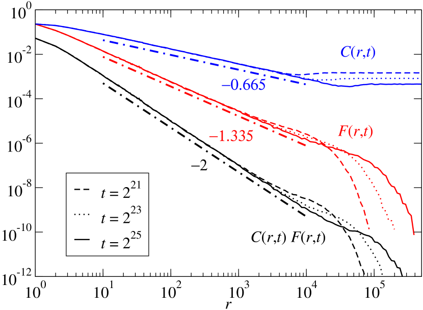
The scaling relation (43) is tested numerically for the NCIM. We measured the correlation functions $F(r,t)$ and $C(r,t)$ numerically in Monte Carlo simulations. Figure 5 presents the numerical data for the system of size $L=2^{20}$ with the parameters $u=1-v=0.3$ and $\bar{u}=\bar{v}=0$. The correlation functions follow a power law in the regime $r\ll t^{1/z}\ll L$. The power law justifies the requirement for the scaling argument. We also plot the product of $C(r,t)$ and $F(r,t)$. It follows the power law with the exponent $-2$, which verifies the scaling relation (43). The same results are obtained from other values of $u$ (details not shown here). Thus, we expect that the cluster man-field approximation leads to the correct scaling relation.

The remaining question is why the cluster mean-field type approximation should be accurate even though the fluctuation is crucial in one dimension. The cluster mean-field approximation has the same spirit as the independent interval approximation Alemany and ben Avraham (1995); Krapivsky and Ben-Naim (1997) which was successful to describe the domain size distribution in reaction diffusion systems. Of course, a successful approximation in one model does not necessarily imply the applicability to any other models. It can be an interesting theoretical challenge to understand the applicability of the cluster mean-field type approximation Eq. (37) which is beyond the scope of this work. We defer this question to later works.

Figure 6: Comparison of the scaling exponent $z\delta$ obtained from the Monte Carlo simulation of Ref. Kim et al. (2013) and the block spin analysis.

Accepting the relation (15), we estimate the critical exponent $\alpha=z\delta$ of the NCIM using the indices $S_{c}$ measured in the previous section. First we need to define the random variable $\rho_{n}$. We set $\rho_{n}=1$ if site $n$ is occupied by a particle irrespective of its species and 0 if site $n$ is empty. With this definition, $P_{1}(b,t)=1-P_{O}(b,t)$ becomes

$$P_{1}(b,t)=P_{A}(b,t)+P_{B}(b,t)+P_{X}(b,t)+P_{Y}(b,t)\ .$$ (44)

It is convenient to rewrite $P_{1}(b,t)$ in terms of two-blocks correlation functions. A block of $\rho_{n}=A$ may be followed by a block of $\rho_{n+1}=O$, $B$, or $Y$. It yields that $P_{A}(b,t)=P_{AO}(b,t)+P_{AB}(b,t)+P_{AY}(b,t)$. One can find the corresponding relations for the others. Thus, we have

$$P_{1}(b,t) = P_{AO}(b,t)+P_{AB}(b,t)+P_{AY}(b,t)$$

$$+ P_{BO}(b,t)+P_{BA}(b,t)+P_{BX}(b,t)$$

$$+ P_{XO}(b,t)+P_{XA}(b,t)+P_{XX}(b,t)$$

$$+ P_{YO}(b,t)+P_{YB}(b,t)+P_{YY}(b,t)\ .$$

Dividing this with $P_{1}(2b,t)=1-P_{OO}(b)$ and taking the limits, we obtain

$$2^{-\alpha}= S_{AO}+S_{AB}+S_{AY}+S_{BO}+S_{BA}+S_{BX}+$$ (45)

$$S_{XO}+S_{XA}+S_{XX}+S_{YO}+S_{YB}+S_{YY}.$$

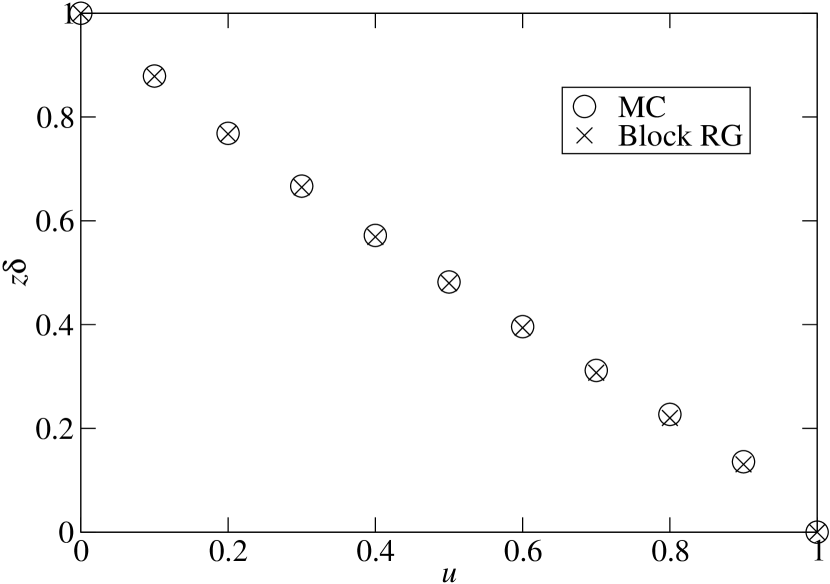
We evaluate the critical exponent $\alpha=z\delta$ by inserting the numerical values of $S_{c}$’s into Eq. (45). For example, we obtain that $\alpha\simeq 0.665$ at $u=0.3$. This value is in perfect agreement with the power-law decay of the correlation function $C(r,t)\sim r^{-\alpha}$ in Fig. 5. It is also consistent with the power-law scaling of $F(r,t)\sim r^{-\theta}$ with $\theta=2-\alpha$. In Fig. 6, the numerical results for $\alpha$, thus obtained, are compared with the values obtained from Monte Carlo simulations in Ref. Kim et al. (2013). Both data are in excellent agreement with each other.

We also studied the scaling relation by assigning $\rho_{n}=1$ if site $n$ is occupied by $A$ and $\rho_{n}=0$ if site $n$ is occupied by $B$ or vacant to get the same result as above (detail not shown). Therefore, we conclude that that block spin analysis supports the claim that the NCIM constitutes a dynamic universality class that is characterized by the continuously varying critical exponents.

V Summary and Discussion

In this paper, we revisited the nonequilibrium chiral Ising model in one dimension using the block renormalization method introduced by Basu and Hinrichsen Basu and Hinrichsen (2011), mainly focusing on the maximal chiral model which was claimed to have continuously varying exponents Kim et al. (2013). First introducing 5 different block spin states reflecting the symmetry of the system as well as the property of having absorbing states, we calculated the asymptotic value of block spin correlation functions which are expected to be universal. It turned out that (universal) ratio of block spin correlation functions varies with a model parameter, which along with the universality hypothesis supports the continuously varying nature of the MCM.

We also provided a microscopic theory about the scaling relation Eq. (15) which associates the ratio of probability that a block with size $b$ is occupied by at least single particle with the critical exponent $z\delta$. First, we clarified necessary conditions that a critical system obeys Eq. (15). Then, we found a relation between two-point correlation functions and the probability that exactly $r$ consecutive sites are empty using cluster mean field type approximation, which is numerically found to be valid for the MCM. Finally, we estimated $z\delta$ using Eq. (15) to find that $z\delta$ is continuously varying and is numerically consistent with the previous numerical results, which again strongly supports that the continuously varying exponents are the inherent feature of the MCM.

Although we neglected the symmetry due to chirality and only kept the feature of having absorbing states when we define $\rho_{n}$ in Sec. IV, we obtained the consistent scaling relation. In this sense, the symmetry of the system is not crucial in the block spin transformation of Basu-Hinrichsen formalism unlike the usual renormalization group theory. The only important feature, at least for models with absorbing states, is whether the block spin can capture the absorbing state properly.