Nonequilibrium noise and current fluctuations at the superconducting phase transition

Abstract

We study non-Gaussian out-of-equilibrium current fluctuations in a mesoscopic NSN circuit at the point of a superconducting phase transition. The setup consists of a voltage-biased thin film nanobridge superconductor (S) connected to two normal-metal (N) leads by tunnel junctions. We find that above a critical temperature fluctuations of the superconducting order parameter associated with the preformed Cooper pairs mediate inelastic electron scattering that promotes strong current fluctuations. Though the conductance is suppressed due to the depletion of the quasiparticle density of states, higher cumulants of current fluctuations are parametrically enhanced. We identify an experimentally relevant transport regime where excess current noise may reach or even exceed the level of thermal noise.

Introduction.– Fluctuations of the order parameter associated with preformed Cooper pairs strongly influence the transport properties of superconductors above the critical temperature $T_{c}$. Owing to extensive research spanning over several decades we have learned a lot about the thermodynamic and kinetic properties in the fluctuation regime Book . In the context of transport, fluctuation-induced corrections to electric, thermal, thermoelectric, and thermomagnetic kinetic coefficients have been rigorously established within the linear response formalism. However, despite its long history, little is known about the nonlinear Dorsey ; LO ; AL or nonequilibrium domains Aronov ; Kogan ; Nagaev . In particular, the answer to the question on how superconducting fluctuations affect the noise or higher-order correlation functions of various observables remains open. We address this outstanding problem by studying excess current noise in a system where a superconductor is tailored to be in the fluctuation regime above $T_{c}$ and driven out of equilibrium by an externally applied voltage. Interestingly, this problem has a very natural connection to another rich field, namely, the full counting statistics (FCS) of electron transfer FCS in mesoscopic systems. It concentrates on finding a probability distribution function for the number of electrons transferred through the conductor during a given period of time. FCS yields all moments of the charge transfer, and in general it encapsulates complete information about electron transport, including the effects of correlations, entanglement, and also information about large rare fluctuations. To access the FCS experimentally is a challenging task, however, great progress has been achieved during the last decade in the field of quantum noise Exp-1 ; Exp-2 ; Exp-3 ; Exp-4 ; Exp-5 ; Exp-6 ; Exp-7 ; Exp-8 ; Exp-9 ; Exp-10 ; Exp-11 ; Exp-12 ; Exp-13 , where new detection schemes have enabled the extension of traditional shot noise measurements to higher-order current correlators.

This work serves a dual purpose. First, we elucidate the effect of superconducting fluctuations on the nonequilibrium transport and derive a cumulant generating function for FCS of current fluctuations in a mesoscopic proximity circuit that contains, as its element, a fluctuating superconductor. We find that, due to a depletion of the quasiparticle density of states, the conductance of the device under consideration is suppressed, however, noise and higher moments of the current fluctuations are enhanced due to inelastic electron scattering in a Cooper channel. It should be stressed that finding the FCS for interacting electrons is a very challenging task, with only a few analytical results known to date Andreev-PRL01 ; Kindermann-PRL03 ; Dima-PRL04 ; Dima-PRL05 ; Kindermann-PRL05 ; Gogolin-PRL05 ; Gutman-PRL10 (see also the review articles Dima-Review-1 ; Dima-Review-2 ).

The second important aspect of this paper is a derivation of the nonequilibrium variant of the time-dependent Ginzburg-Landau action (TDGL). The conventional paradigm behind TDGL phenomenology TDGL and its subsequent generalizations TDGL-1 ; TDGL-2 ; TDGL-3 ; TDGL-4 ; TDGL-5 ; TDGL-6 is to assume that electronic (quasiparticle) degrees of freedom are at equilibrium and concentrate on the dynamics of the order parameter field. While leading to correct static averages, fluctuation-dissipation relations, and gauge invariance, this way of handling the problem fails to provide any prescription for calculating the higher moments of observables, even at equilibrium. Furthermore, existing theories exclude the stochastic nature of electron scattering on the order parameter fluctuations. Technically, the inclusion of such effects should result in stochastic noise terms (Langevin forces) which have a feedback on superconducting fluctuations. Below we elaborate on the methodology that includes all these effects.

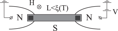
Figure 1: The layout of a mesoscopic NISIN proximity circuit under voltage bias, magnetic field, and at a temperature above $T_{c}$ of a superconductor.

Model and results.– We consider a superconducting diffusive wire (nanobridge) of length $L$ connected to two normal reservoirs by tunnel junctions with dimensionless conductances $g_{1}$ and $g_{2}$, thus forming a NISIN-structure (Fig. 1). For the conductance of the wire we assume $g_{W}>g_{1,2}$ and, moreover, $g_{1,2}\gg 1$, so that charging effects can be neglected. The system is driven out of equilibrium by the finite bias $eV$, and we will limit ourselves to the regime $T-T_{c}\lesssim eV\ll T_{c}$. We also consider an externally applied magnetic field $H$, which leads to dephasing of the Cooper pairs due to orbital effects. We concentrate on the temperature regime in the immediate vicinity of the critical temperature of a superconductor. In this case, electron transport is dominated by interaction effects in the Cooper channel, which are singular in $\Delta T=T-T_{c}$. Finally, we assume $L\lesssim\xi(T)\simeq\sqrt{D/(T-T_{c})}$, where $\xi$ is a superconducting coherence length and $D$ is a diffusion coefficient in the wire. This assumption greatly simplifies the problem by making it effectively zero dimensional when neglecting gradient terms in the effective low-energy action. We note that such devices are readily available in experiments Exp-14 ; Exp-15 ; Chan-PRL05 ; Chan-PRL09 ; Chen-PRL09 ; Chen-PRB11 ; Aref-PRB12 ; Li-PRB11 ; Kamenev_NPhys14 and find their practical implementation as superconducting hot electron bolometers Prober ; Exp-Grenoble .

Our goal is to derive the cumulant generation function (CGF) ${\cal F}(\chi)$ for the irreducible moments of current fluctuations. It is defined as a logarithm of the nonequilibrium partition function, ${\cal F}(\chi)=-\ln\mathcal{Z}(\chi)$, where the counting field $\chi$ is the variable conjugated to the classical part of the current $I$. Derivatives of ${\cal F}(\chi)$ give the average value of the current, shot noise, and higher-order moments $C_{n}$ of charge transfer during a long observation time $t_{0}$.

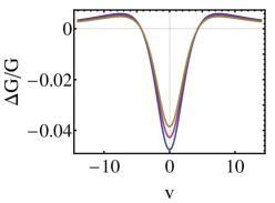
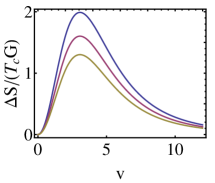
Figure 2: Fluctuation-induced correction to conductance $\Delta G$ normalized to the normal conductance $G$ (left), and normalized fluctuation-induced nonequilibrium excess current noise in units of thermal noise power $T_{c}G$ (right), plotted vs bias voltage $v=eV/\sqrt{T_{c}\Delta T}$ for $\Delta T=\delta$, $g=2.5\times 10^{3}$ and $\Gamma/T_{c}=0.25,0.5,0.75$.

In the normal state away from $T_{c}$, where superconducting correlations are negligible, the above device represents a double tunnel junction. In this case CGF is easy to compute (see, e.g., Ref. Dima-Review-1 ). The effects of a Coulomb interaction on conductance and current noise in a similar setup have been previously addressed on the basis of the quantum kinetic approach equation Ahmadian-PRB05 ; Catelani-PRB07 . Superconducting correlations in the vicinity of $T_{c}$ strongly affect CGF already at low bias, $eV\ll T_{c}$. We delegate a derivation to the end of the paper and first present our main result,

$${\cal F}(\chi)=-t_{0}T_{c}\mathcal{E}\left[1-\sqrt{1-2\left(\chi^{2}-\frac{ieV\chi}{T_{c}}\right)\frac{\phi+\eta\mathcal{E}}{\mathcal{E}^{2}}}\right],$$ (1)

which accounts for inelastic scattering of electrons on superconducting fluctuations while traversing across the wire. The proximity to a superconducting transition is controlled by the function

$$\mathcal{E}(\Delta T,V)=a\frac{\Delta T}{T_{c}}+b\frac{(eV)^{2}}{T^{2}_{c}},\quad a=\frac{8}{\pi},\quad b=\alpha_{1}\alpha_{2}\frac{14\zeta(3)}{\pi^{3}},$$ (2)

where $\alpha_{k}=g_{k}/(g_{1}+g_{2})$ and $\zeta$ is the Riemann zeta function. At finite magnetic field the critical temperature is downshifted according to the law $\ln(T_{c}/T_{c0})=\psi\big{(}\frac{1}{2}\big{)}-\psi\big{(}\frac{1}{2}+\frac{\Gamma}{4\pi T_{c}}\big{)}$, where $T_{c0}=T_{c}(H=0)$, $\Gamma=E_{Th}+\tau^{-1}_{H}$ and $\psi$ is the digamma function. Thouless energy $E_{Th}=(g_{1}+g_{2})\delta/4\pi$ is defined through the mean level spacing in the wire $\delta$, while the dephasing time $\tau^{-1}_{H}\simeq(D/L^{2})(\Phi/\Phi_{0})^{2}\propto H^{2}$ is due to orbital effects of the perpendicular magnetic field, where $\Phi$ is a total magnetic flux through the wire and $\Phi_{0}$ is the flux quantum. The two dimensionless functions in Eq. (1) are defined as follows:

$$\phi=-\frac{\alpha_{1}\alpha_{2}}{\pi^{3}}\left(\frac{E_{Th}}{T_{c}}\right)\psi^{\prime\prime}\left(\frac{1}{2}+\frac{\Gamma}{4\pi T_{c}}\right),$$ (3a)

$$\eta=\frac{2\alpha_{2}\alpha_{2}}{\pi^{3}}\left[\frac{E_{Th}}{\pi\Gamma}\psi^{\prime\prime\prime}\left(\frac{1}{2}+\frac{\Gamma}{4\pi T_{c}}\right)-\psi^{\prime\prime}\left(\frac{1}{2}+\frac{\Gamma}{4\pi T_{c}}\right)\right].$$ (3b)

The effect of fluctuations is the most singular provided that $E_{Th}\gg\Delta T$ where $\phi\gg\eta\mathcal{E}$. In this case Eq. (1) yields a conductance correction

$$\frac{\Delta G}{G_{Q}}=\frac{2\alpha_{1}\alpha_{2}}{\pi^{2}}\left(\frac{E_{Th}}{\Delta T}\right)\psi^{\prime\prime}\left(\frac{1}{2}+\frac{\Gamma}{4\pi T_{c}}\right)\frac{a-bv^{2}}{(a+bv^{2})^{2}},$$ (4)

where we introduced a notation $v=eV/\sqrt{T_{c}\Delta T}$. This result is plotted in Fig. 2 (left) for a certain choice of parameters versus bias voltage and has a BCS-like density of states profile (note that $\Delta G$ is actually negative since $\psi^{\prime\prime}<0$). The latter should not be surprising since superconducting fluctuations deplete energy states near the Fermi level, which leads to a zero-bias anomaly. In the same limit we find an excess current noise power,

$$\frac{\Delta S_{I}}{G_{Q}T_{c}}=\frac{4\alpha^{2}_{1}\alpha^{2}_{2}}{\pi^{5}}\left[\psi^{\prime\prime}\left(\frac{1}{2}+\frac{\Gamma}{4\pi T_{c}}\right)\right]^{2}\!\!\left(\frac{E_{Th}}{\Delta T}\right)^{2}\!\!\frac{v^{2}}{(a+bv^{2})^{3}},$$ (5)

which is plotted in Fig. 2 (right). The low frequency dispersion of the noise is set by $\omega=\mathrm{max}\{\Delta T,(eV)^{2}/T_{c}\}$. From Eq. (1) one can extract the $n^{th}$-moment of the current fluctuations which progressively display more singular behavior,

$$C_{n}=\langle I(\omega_{1})\ldots I(\omega_{n})\rangle_{\omega_{k}\to 0}\!\simeq e^{n-2}G_{Q}T_{c}\!\left(\frac{E_{Th}}{\Delta T}\right)^{n}\!\!\left(\frac{T_{c}}{\Delta T}\right)^{n/2-1}.$$ (6)

We interpret this result as bunching of electrons due to slow time-dependent fluctuations of the order parameter, which result in a long avalanches of charges and thus parametrically enhanced current fluctuations.

This conclusion is substantiated by the direct analysis of the current probability distribution defined by $P(I)=(2\pi)^{-1}\int_{-\pi}^{\pi}\exp\{-{\cal F}(\chi)+i\chi(It_{0}/e)\}d\chi$. We estimate this integral using the saddle point method by rotating the integration contour to complex $\chi$. The typical result is plotted in Fig. 3. The resulting distribution has a long exponential tail $P(I)\propto\exp\{-\lambda(It_{0}/e)\}$ for positive currents $I$ originating from the branch point $\chi=i\lambda$ of the CGF and describing avalanches of transferred charges. In the limit $E_{\rm Th}\gg\Delta T$ one finds $\lambda=(T_{c}/eV)(\mathcal{E}^{2}/2\phi)$, which gives an estimate $\lambda\sim(1/g)(\delta/T_{c})^{1/2}\ll 1$ at the direct vicinity of the phase transition when $\Delta T\sim\delta$ and $v\sim 1$. The latter result is in agreement with Eq. (6). We note that parametric enhancement of current fluctuations is a universal phenomenon whenever soft modes are present in the system, and is known to occur, e.g., in interacting diffusive mesoscopic wires Dima-PRL04 or in molecular junctions Utsumi:2013 .

Estimates.– Let us now discuss the experimentally relevant parameters to observe the effect and estimate its actual magnitude. The maximal value of the nonequilibrium excess current noise normalized to the thermal noise at $T_{c0}$ that follows from Eq. (5) is

$$\left(\frac{\Delta S_{I}}{GT_{c0}}\right)_{\mathrm{max}}\simeq\frac{1}{25g}\left(\frac{E_{Th}}{\Delta T}\right)^{2}.$$ (7)

When finding this estimate we took symmetric structure $\alpha_{1}=\alpha_{2}=1/2$, used $\psi^{\prime\prime}(1/2)=-14\zeta(3)$ and assumed $\Gamma/4\pi T_{c}\ll 1$. This condition will be justified below. The minimal allowed $\Delta T$ in our theory is limited by the mean level spacing. Indeed, since $E_{Th}/\Delta T=g/2\pi$ at $\Delta T=\delta$, then the fluctuation-induced correction to conductance $\Delta G$ in Eq. (4) already reaches its bare value and thus our approach breaks down for the lower $\Delta T$. At that bound the noise remains parametrically enhanced, $(\Delta S_{I}/GT_{c0})_{\mathrm{max}}\simeq g/100\pi^{2}$, since $g\gg 1$, however, a large numerical factor in the denominator significantly diminishes the actual magnitude of the effect. Now we look for realistic numbers. For the layout design in Fig. 1 we assume a wire of length $L\simeq 0.5\mu$m and width $w\simeq 100$nm be made of a two-dimensional film of thickness $d\simeq 10$nm. For aluminum nanowires the typical diffusion coefficient is $D\simeq 10^{2}$cm²s^-1, the Fermi velocity is $v_{F}=2\cdot 10^{8}$cm/s, and resistivity $\rho\simeq 2\mu\Omega$cm. These numbers provide a Thouless energy $E_{Th}=D/L^{2}\simeq 0.3$K, a mean free path $l=3D/v_{F}\simeq 15$nm, a diffusive coherence length at zero temperature $\xi=\sqrt{\xi_{0}l}\simeq 440$nm, where $\xi_{0}=v_{F}/T_{c0}\simeq 1.3\mu$m for the bulk aluminum $T_{c0}=1.2$K, and a sheet resistance $\rho_{\Box}=\rho/d\simeq 2\Omega$. The latter translates into the normal wire resistance $R_{W}=\rho_{\Box}L/w\simeq 10\Omega$ and the dimensionless conductance $g=1/G_{Q}R_{W}\simeq 2.5\cdot 10^{3}$ of the nanostructure. The corresponding mean level spacing is $\delta=2\pi E_{Th}/g\simeq 0.75$mK while $\Gamma/T_{c0}\simeq 0.25$. Finally, the realistic estimate for maximal nonequilibrium noise above its thermal level is $(\Delta S_{I}/GT_{c0})_{\mathrm{max}}\simeq 2$, as shown in Fig. 2 (right). Similar estimates can be carried out for zinc and lead nanowires. All these parameters are within the reach of current nanoscale fabrication technology and high precision measurements.

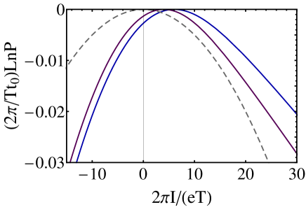
Figure 3: The logarithm of probability $P(I)$ to measure current fluctuations plotted vs the current $I$. The parameters are the same as in Fig. 2, with $\Gamma/T_{c}=0.25$. Top curve: $v=3.0$; middle curve:$v=1.5$; dotted curve: $v=0$ (Gaussian thermal fluctuation).

Formalism.– As a technical tool to derive Eq. (1), we use the Keldysh technique built into the framework of the nonlinear-sigma-model (NL$\sigma$M) NLSM-1 ; NLSM-2 ; NLSM-3 . For the above specified conditions, separation of the length scales $l\ll\xi(0)\ll L\ll\xi(T)$ implies a diffusive limit and the quantum action of the device under consideration (Fig. (1)) is given by the following expression $\mathcal{S}=\mathcal{S}_{Q}+\mathcal{S}_{\Delta}+\mathcal{S}_{T}+\mathcal{S}_{H}$, where

$$\mathcal{S}_{Q}=\frac{i\pi}{\delta}\mathrm{Tr}\big{(}-\hat{\tau}_{3}\partial_{t}\hat{Q}+i\hat{\Delta}\hat{Q}\big{)},\quad\mathcal{S}_{\Delta}=-\frac{2}{\lambda\delta}\mathrm{Tr}\big{(}\vec{\Delta}^{\dagger}\hat{\sigma}_{1}\vec{\Delta}\big{)},$$ (8a)

$$\mathcal{S}_{T}=\frac{i}{16}\sum_{k=1,2}g_{k}\mathrm{Tr}\big{\{}\hat{Q}^{[\chi]}_{k},\hat{Q}\big{\}},\quad\mathcal{S}_{H}=\frac{i\pi}{8\delta\tau_{H}}\mathrm{Tr}\big{(}\hat{\tau}_{3}\hat{Q}\big{)}^{2}.$$ (8b)

Here $\delta$ is the mean level spacing in the island, and $\lambda$ is the coupling constant in the Cooper channel. The two sets of Pauli matrices $\hat{\tau}_{i}$ and $\hat{\sigma}_{i}$ are operating in the Gor’kov-Nambu ($N$) and Keldysh ($K$) subspaces, respectively. Additionally, $\mathrm{Tr}(\ldots)$ implies a trace over all matrices and continuous indices while curly brackets $\{,\}$ stand for the anticommutator. The action $\mathcal{S}_{Q}$ represents coupling between the $\hat{Q}_{tt^{\prime}}$-matrix field and the superconducting order parameter field $\hat{\Delta}(t)$. The former is essentially a local in space electronic Green’s function in the island which is a matrix in $K\otimes N\otimes T$ (time) spaces. The superconducting part of the action $\mathcal{S}_{\Delta}$ stems from the Hubbrd-Stratonovich decoupling of a bare four-fermion BCS interaction term, which is done by introducing the $\hat{\Delta}$-field. The action is subject to the nonlinear constraint $\hat{Q}^{2}=1$. As usual for the Keldysh theory Review , all fields come in doublets of classical and quantum components. The former obey equations of motion, and the latter serve to generate these equations along with the corresponding stochastic noise terms. In particular,

$$\hat{\Delta}=\hat{\Delta}^{c}\hat{\sigma}_{0}+\hat{\Delta}^{q}\hat{\sigma}_{3},\quad\hat{\Delta}^{\alpha}=\left(\begin{array}[]{cc}0&\Delta^{\alpha}\\ -\Delta^{*\alpha}&0\end{array}\right)_{N},\quad\vec{\Delta}=\left(\begin{array}[]{c}\Delta^{c}\\ \Delta^{q}\end{array}\right).$$ (9)

The action $\mathcal{S}_{T}$ describes the coupling of the $\hat{Q}$-matrix in the island to those in the leads,

$$\hat{Q}^{[\chi]}_{k}=\left(\begin{array}[]{cc}\hat{h}_{k}&-(1-\hat{h}_{k})e^{i\chi_{k}\hat{\tau}_{3}}\\ -(1+\hat{h}_{k})e^{-i\chi_{k}\hat{\tau}_{3}}&-\hat{h}_{k}\end{array}\right)_{K}\hat{\tau}_{3},$$ (10)

where $\hat{h}_{k}=h(\varepsilon-eV_{k}\hat{\tau}_{3})=\tanh\big{(}\frac{\varepsilon-eV_{k}\hat{\tau}_{3}}{2T}\big{)}$ is the distribution function and $\chi_{k}$ is the counting field. The latter is essentially a quantum component of the vector potential which serves to generate observable current and its higher moments. Finally, the $\mathcal{S}_{H}$ part of the action accounts for the dephasing term of Cooper pairs due to the magnetic field. The action $\mathcal{S}[Q,\Delta,\chi]$ defines the nonequilibrium partition function via the functional integral over all possible realizations of $\hat{Q}$ and $\hat{\Delta}$,

$$\mathcal{Z}(\chi)=\int\mathcal{D}[Q,\Delta]\exp(i\mathcal{S}[Q,\Delta,\chi]).$$ (11)

Knowledge of $\mathcal{Z}$ yields all desired cumulants for current fluctuation by the simple differentiation $\langle I^{n}\rangle=(e/t_{0})^{n}(-i\partial_{\chi})^{n}\ln\mathcal{Z}(\chi)$.

Technicalities.– When computing the path integral in Eq. (11) we need to identify such a configuration of the $\hat{Q}$-matrix field that realizes the saddle point of the action Eq. (8a). For this purpose one needs a parametrization of the $\hat{Q}$-field which explicitly resolves the nonlinear constraint $\hat{Q}^{2}=1$. We adopt the exponential parametrization $\hat{Q}=e^{-i\hat{W}}\hat{Q}_{0}e^{i\hat{W}}$ with $\{\hat{W},\hat{Q}_{0}\}=0$, where the matrix multiplication in the time space is implicitly assumed. A new matrix field $\hat{W}_{tt^{\prime}}$ accounts for the rapid fluctuations of $\hat{Q}$ associated with the electronic degrees of freedom and is to be integrated out, while $\hat{Q}_{0}$ is the stationary Green’s function. Minimizing the action Eq. (8a) with respect to $\hat{W}$, one finds the following saddle point equation for $\hat{Q}_{0}$,

$$\frac{\delta}{8\pi}\sum_{k}g_{k}\big{[}\hat{Q}_{0},\hat{Q}^{[\chi]}_{k}\big{]}=-\big{\{}\hat{\tau}_{3}\partial_{t},\hat{Q}_{0}\big{\}}+i\big{[}\hat{\Delta},\hat{Q}_{0}\big{]}+\frac{1}{4\tau_{H}}\big{[}\hat{\tau}_{3}\hat{Q}_{0}\hat{\tau}_{3},\hat{Q}_{0}\big{]}$$ (12)

which is merely a zero-dimensional version of the Usadel equation. In the stationary case and without superconducting correlations, Eq. (12) is solved by such a $\hat{Q}_{0}$ that nullifies the commutator in the left-hand side. This immediately suggests a solution for $\hat{Q}_{0}$ that has to be chosen as a linear combination of the $\hat{Q}$-matrices in the leads,

$$\hskip-14.22636pt\hat{Q}_{0}=\left(\alpha_{1}\hat{Q}^{[\chi]}_{1}+\alpha_{2}\hat{Q}^{[\chi]}_{2}\right)/\sqrt{N_{\chi}},$$ (13)

$$\hskip-14.22636ptN_{\chi}=\frac{1}{(g_{1}+g_{2})^{2}}\left(g^{2}_{1}+g^{2}_{2}+g_{1}g_{2}\big{\{}\hat{Q}^{[\chi]}_{1},\hat{Q}^{[\chi]}_{2}\big{\}}\right),$$ (14)

where the factor $N_{\chi}$ ensures proper normalization. If one now uses Eqs. (13) and (14) back in the action Eq. (8a), then the partition function of the normal double tunnel junction follows immediately, in agreement with Ref. Dima-Review-1 .

The next step is to integrate out the fluctuations around the saddle point. To this end, we linearize Eq. (12) with respect to $\delta\hat{Q}_{0}=2i\hat{Q}_{0}\hat{W}$, and solve for the Cooperon matrix field $\hat{W}$ to linear order in the superconducting field $\hat{\Delta}$ by passing to Fourier space to invert the matrix equation. The result is

$$\hat{W}_{\varepsilon\varepsilon^{\prime}}=\frac{i}{2}\frac{i\Gamma_{\chi}+(\varepsilon+\varepsilon^{\prime})\hat{\tau}_{3}\hat{Q}_{0}}{\Gamma^{2}_{\chi}+(\varepsilon+\varepsilon^{\prime})^{2}}\big{[}\hat{\Delta},\hat{Q}_{0}\big{]},$$ (15)

where $\Gamma_{\chi}=\tau^{-1}_{H}+E_{Th}\sqrt{N_{\chi}}$. Integrating over $\hat{W}$ at the Gaussian level in Eq. (11), $\int D[W]\exp(i\mathcal{S}[W,\Delta,\chi])=\exp(i\mathcal{S}[\Delta,\chi])$, one arrives at the effective action written in terms of the superconducting order parameter only,

$$\mathcal{S}[\Delta,\chi]=\mathcal{S}_{a}[\Delta,\chi]+\mathcal{S}_{b}[\Delta,\chi]+\mathcal{S}_{\Delta},$$ (16a)

$$\mathcal{S}_{a}=\frac{\pi}{2\delta}\mathrm{Tr}\left(\mathcal{\hat{C}}^{a}_{\varepsilon\varepsilon^{\prime}}(\hat{Q}_{0}(\varepsilon)\hat{\Delta}_{\varepsilon-\varepsilon^{\prime}}\hat{\Delta}_{\varepsilon^{\prime}-\varepsilon}+\hat{\Delta}_{\varepsilon-\varepsilon^{\prime}}\hat{\Delta}_{\varepsilon^{\prime}-\varepsilon}\hat{Q}_{0}(\varepsilon^{\prime}))\right),$$ (16b)

$$\mathcal{S}_{b}=\frac{\pi}{2\delta}\mathrm{Tr}\left(\mathcal{\hat{C}}^{b}_{\varepsilon\varepsilon^{\prime}}(\hat{\Delta}_{\varepsilon-\varepsilon^{\prime}}\hat{\Delta}_{\varepsilon^{\prime}-\varepsilon}-\hat{\Delta}_{\varepsilon-\varepsilon^{\prime}}\hat{Q}_{0}(\varepsilon^{\prime})\hat{\Delta}_{\varepsilon^{\prime}-\varepsilon}\hat{Q}_{0}(\varepsilon))\right),$$ (16c)

where $\hat{\mathcal{C}}^{a}_{\varepsilon\varepsilon^{\prime}}=i(\varepsilon+\varepsilon^{\prime})\hat{\tau}_{3}/[(\varepsilon+\varepsilon^{\prime})^{2}+\Gamma^{2}_{\chi}]$ and $\hat{\mathcal{C}}^{b}_{\varepsilon\varepsilon^{\prime}}=\Gamma_{\chi}\hat{\tau}_{0}/[(\varepsilon+\varepsilon^{\prime})^{2}+\Gamma^{2}_{\chi}]$ are Cooperon propagators. For technical reasons of convenience, with the intermediate steps of the calculations we choose to work in the gauge $\chi_{1}=\alpha_{2}\chi$ and $\chi_{2}=-\alpha_{1}\chi$, and similarly for the voltages $V_{1}=\alpha_{2}V$ and $V_{2}=-\alpha_{1}V$. Carrying out matrix products, traces, and integrations with the help of Eqs. (9), (10), and (13), one eventually finds

$$\mathcal{S}[\Delta,\chi]=\frac{\pi}{4\delta}\mathrm{Tr}\left(\vec{\Delta}^{\dagger}_{-\omega}\hat{\Pi}_{\omega}(V,\Delta T,\chi)\vec{\Delta}_{\omega}\right),$$ (17a)

$$\hat{\Pi}_{\omega}=\left(\begin{array}[]{cc}-i\chi^{2}_{v}\phi&\mathcal{E}-i\omega/T_{c}-\chi^{2}_{v}\eta\\ \mathcal{E}+i\omega/T_{c}-\chi^{2}_{v}\eta&2i\end{array}\right).$$ (17b)

Here we have used the notation $\chi^{2}_{v}=\chi^{2}-ieV\chi/T_{c}$. Equation (17a) represents a time-dependent Ginzburg-Landau action for nonequilibrium superconducting fluctuations. Off-diagonal elements (retarded and advanced blocks) of the propagator matrix $\hat{\Pi}_{\omega}$ carry information about the excitation spectrum of fluctuations. The Keldysh block (quantum-quantum element of the matrix $\propto\Delta^{q}\Delta^{*q}$) ensures fluctuation-dissipation relations. The anomalous classical-classical block accounts for the feedback of stochastic Langevin forces of fluctuations due to the nonequilibrium quasiparticle background.

Performing the remaining path integration over $\Delta$ in Eq. (11) with the action from Eq. (17a), one realizes that the corresponding cumulant generation function for current fluctuations is governed by the determinant of the Ginzburg-Landau propagator [Eq. (17b)], namely, $\ln\Delta\mathcal{Z}\propto\mathop{\rm det}\nolimits\hat{\Pi}_{\omega}$. We regularize $\mathop{\rm det}\nolimits\hat{\Pi}_{\omega}$ by normalizing it to itself taken at zero counting field, $\mathop{\rm det}\nolimits\hat{\Pi}_{\omega}\to\mathop{\rm det}\nolimits\hat{\Pi}_{\omega}(\chi)/\mathop{\rm det}\nolimits\hat{\Pi}_{\omega}(0)$, and thereby find

$$\ln\Delta\mathcal{Z}=t_{0}\int\frac{d\omega}{2\pi}\ln\left[1-\frac{2\chi^{2}_{v}(\phi+\mathcal{E}\eta)}{\mathcal{E}^{2}+\omega^{2}/T^{2}_{c}}\right]$$ (18)

which upon final integration reduces to Eq. (1). From the structure of the effective action (16a), and also relying on previous studies Ahmadian-PRB05 ; TDGL-6 , one can identify the essential physical processes affecting conductance and noise. The first $S_{a}$ term in the effective action corresponds to the density of states effect. Superconducting fluctuations suppress the quasiparticle density of states near the Fermi level that translate into a zero-bias conductance dip Dos . The second $S_{b}$ term of the action corresponds to the inelastic Maki-Thompson process Maki-Thompson , which can be thought of as resonant electron scattering on the preformed Cooper pairs. The combined effect of the two processes has a profound implication for the higher cumulants of the current noise. The final remark is that the Aslamazov-Larkin fluctuational correction Aslamazov-Larkin is absent in our case since we are considering a zero-dimensional limit while the latter relies essentially on the spatial gradients of the superconducting order parameter.

Acknowledgments.– We would like to thank M. Reznikov for motivating this study and A. Kamenev for a number of useful discussions. The work by D. B. was supported by SFB/TR 12 of the Deutsche Forschungsgemeinschaft. A. L. acknowledges support from NSF Grant No. ECCS-1407875, and the hospitality of the Karlsruhe Institute of Technology where this work was finalized.

References

- (1) A. I. Larkin and A. Varlamov, Theory of Fluctuations in Superconductors (Clarendon Press, Oxford, 2005).
- (2) A. T. Dorsey, Phys. Rev. B 43, 7575 (1991).
- (3) A. I. Larkin and Yu. N. Ovchinnikov, JETP 92, 519 (2001).
- (4) A. Levchenko, Phys. Rev. B 78, 104507 (2008); ibid. 81, 012507 (2010).
- (5) A. G. Aronov and R. Katilyus, Sov. Phys. JETP 41, 1106 (1976).
- (6) Sh. M. Kogan and K. E. Nagaev, Sov. Phys. JETP 67, 579 (1988).
- (7) K. E. Nagaev, JETP Lett. 52, 289 (1990); Physica C 184, 149 (1991).
- (8) Y. V. Nazarov (ed.), Quantum Noise in Mesoscopic Physics, (Kluwer Academic Publishers, 2003).
- (9) B. Reulet, J. Senzier, and D. E. Prober, Phys. Rev. Lett. 91, 196601 (2003).
- (10) Yu. Bomze, G. Gershon, D. Shovkun, L. S. Levitov, and M. Reznikov, Phys. Rev. Lett. 95, 176601 (2005).
- (11) S. Gustavsson, R. Leturcq, B. Simovic, R. Schleser, T. Ihn, P. Studerus, K. Ensslin, D. C. Driscoll, and A. C. Gossard, Phys. Rev. Lett. 96, 076605 (2006).
- (12) T. Fujisawa, T. Hayashi, R. Tomita, and Y. Hirayama, Science 312, 1634 (2006).
- (13) A. V. Timofeev, M. Meschke, J. T. Peltonen, T. T. Heikkila, and J. P. Pekola, Phys. Rev. Lett. 98, 207001 (2007).
- (14) E. V. Sukhorukov, A. N. Jordan, S. Gustavsson, R. Leturcq, T. Ihn, and K. Ensslin, Nat. Phys. 3, 243 (2007).
- (15) G. Gershon, Yu. Bomze, E. V. Sukhorukov, and M. Reznikov, Phys. Rev. Lett. 101, 016803 (2008).
- (16) C. Flindt, C. Fricke, F. Hohls, T. Novotny, K. Netocny, T. Brandes, and R. J. Haug, Proc. Natl. Acad. Sci. U.S.A. 106, 10116 (2009).
- (17) J. Gabelli and B. Reulet, Phys. Rev. B 80, 161203(R) (2009).
- (18) S. Gustavsson, R. Leturcq, M. Studer, I. Shorubalko, T. Ihn, K. Ensslin, D. C. Driscoll, and A. C. Gossard, Surf. Sci. Rep. 64, 191 (2009).
- (19) Q. Le Masne, H. Pothier, N. O. Birge, C. Urbina, and D. Esteve, Phys. Rev. Lett. 102, 067002 (2009).
- (20) N. Ubbelohde, C. Fricke, C. Flindt, F. Hohls, and R. J. Haug, Nat. Commun. 3, 612 (2012).
- (21) V. F. Maisi, D. Kambly, C. Flindt, and J. P. Pekola, Phys. Rev. Lett. 112, 036801 (2014).
- (22) A. V. Andreev and E. G. Mishchenko, Phys. Rev. B 64, 233316 (2001).
- (23) M. Kindermann and Yu. V. Nazarov, Phys. Rev. Lett. 91, 136802 (2003).
- (24) D. A. Bagrets, Phys. Rev. Lett. 93, 236803 (2004).
- (25) D. A. Bagrets and Yu. V. Nazarov, Phys. Rev. Lett. 94, 056801 (2005).
- (26) M. Kindermann and B. Trauzettel, Phys. Rev. Lett. 94, 166803 (2005).
- (27) A. Komnik and A. O. Gogolin, Phys. Rev. Lett. 94, 216601 (2005).
- (28) D. B. Gutman, Y. Gefen, and A. D. Mirlin, Phys. Rev. Lett. 105, 256802 (2010).
- (29) D. A. Bagrets and Yu. V. Nazarov, in Quantum Noise, edited by Yu. V. Nazarov and Ya. M. Blanter (Kluwer, 2003).
- (30) D. A. Bagrets, Y. Utsumi, D. S. Golubev, G. Schön, Fortschritte der Physik 54, 917 (2006).
- (31) L. P. Gor’kov and G. M. Eliashberg, Sov. Phys. JETP 27, 328 (1968).
- (32) L. Kramer and R. J. Watts-Tobin, Phys. Rev. Lett. 40, 1041 (1978).
- (33) C.-R. Hu, Phys. Rev. B 21, 2775 (1980).
- (34) J. J. Krempasky and R. S. Thompson, Phys. Rev. B 32, 2965 (1985).
- (35) A. Otterlo, D. S. Golubev, A. D. Zaikin, and G. Blatter, Eur. Phys. J. B 10, 131 (1999).
- (36) I. V. Yurkevich and I. V. Lerner, Phys. Rev. B 63, 064522 (2001).
- (37) A. Levchenko and A. Kamenev, Phys. Rev. B 76, 094518 (2007).
- (38) J. T. Peltonen, P. Virtanen, M. Meschke, J. V. Koski, T. T. Heikkilä, and J. P. Pekola, Phys. Rev. Lett. 105, (2010).
- (39) N. Vercruyssen, T. G. A. Verhagen, M. G. Flokstra, J. P. Pekola, and T. M. Klapwijk, Phys. Rev. B 85, 224503 (2012).
- (40) M. Tian, N. Kumar, S. Xu, J. Wang, J. S. Kurtz, and M. H. W. Chan, Phys. Rev. Lett. 95, 076802 (2005).
- (41) J. Wang, C. Shi, M. Tian, Q. Zhang, N. Kumar, J. K. Jain, T. E. Mallouk, and M. H. W. Chan, Phys. Rev. Lett. 102, 247003 (2009).
- (42) Y. Chen, S. D. Snyder, and A. M. Goldman, Phys. Rev. Lett. 103, 127002 (2009).
- (43) Y. Chen, Y.-H. Lin, S. D. Snyder, and A. M. Goldman, Phys. Rev. B 83, 054505 (2011).
- (44) T. Aref, A. Levchenko, V. Vakaryuk, and A. Bezryadin Phys. Rev. B 86, 024507 (2012).
- (45) P. Li, P. M. Wu, Y. Bomze, I. V. Borzenets, G. Finkelstein, and A. M. Chang, Phys. Rev. B 84, 184508 (2011).
- (46) Y. Chen, Y.-H. Lin, S. D. Snyder, A. M. Goldman, A. Kamenev, Nature Physics, (2014)
- (47) D. E. Prober, Appl. Phys. Lett. 62, 2119 (1992).
- (48) R. Romestain, B. Delaet, P. Renaud-Goud, I. Wang, C. Jorel, J.-C. Villegier and J.-Ph. Poizat, New J. Phys. 6 129 (2004).
- (49) Y. Ahmadian, G. Catelani, and I. L. Aleiner, Phys. Rev. B 72, 245315 (2005).
- (50) G. Catelani and M. G. Vavilov, Phys. Rev. B 76, 201303(R) (2007).
- (51) Y. Utsumi, O. Entin-Wohlman, A. Ueda, and A. Aharony, Phys. Rev. B 87, 115407 (2013).
- (52) A. Kamenev and A. Andreev, Phys. Rev. B 60, 2218 (1999).
- (53) M. V. Feigel’man, A. I. Larkin, and M. A. Skvortsov, Phys. Rev. B 61, 12361 (2000).
- (54) D. B. Gutman, A. D. Mirlin, and Y. Gefen, Phys. Rev. B 71, 085118 (2005).
- (55) A. Kamenev and A. Levchenko, Adv. in Phys. 58, 197 (2009).
- (56) E. Abrahams, M. Redi, and J. W. Woo, Phys. Rev. B 1, 208 (1970).
- (57) K. Maki, Prog. Theor. Phys. 39, 897 (1968); R. S. Thompson, Phys. Rev. B 1, 327 (1970).
- (58) L. G. Aslamazov and A. I. Larkin, Fiz. Tverd. Tela 10, 1104 (1968) [Sov. Phys. Solid. State 10, 875 (1968)].