The direct collapse of a massive black hole seed under the influence of an anisotropic Lyman-Werner source

Abstract

The direct collapse model of supermassive black hole seed formation requires that the gas cools predominantly via atomic hydrogen. To this end we simulate the effect of an anisotropic radiation source on the collapse of a halo at high redshift. The radiation source is placed at a distance of 3 kpc (physical) from the collapsing object and is set to emit monochromatically in the center of the Lyman-Werner (LW) band. The LW radiation emitted from the high redshift source is followed self-consistently using ray tracing techniques. Due to self-shielding, a small amount of $\rm{H_{2}}$ is able to form at the very center of the collapsing halo even under very strong LW radiation. Furthermore, we find that a radiation source, emitting $>10^{54}\ (\sim 10^{3}\ \rm{J_{21}})$ photons per second is required to cause the collapse of a clump of $\rm{M\sim 10^{5}}$ $\rm{M_{\odot}}$. The resulting accretion rate onto the collapsing object is $\sim 0.25$ $\rm{M_{\odot}}~{}$$\rm{yr^{-1}}$. Our results display significant differences, compared to the isotropic radiation field case, in terms of $\rm{H_{2}}$ fraction at an equivalent radius. These differences will significantly effect the dynamics of the collapse. With the inclusion of a strong anisotropic radiation source, the final mass of the collapsing object is found to be $\rm{M\sim 10^{5}}$ $\rm{M_{\odot}}$. This is consistent with predictions for the formation of a supermassive star or quasi-star leading to a supermassive black hole.

1. Introduction

Observations of supermassive black holes (SMBH) at redshifts greater than $z\gtrsim 6$ (Fan, 2004; Fan et al., 2006; Mortlock et al., 2011; Venemans et al., 2013) has led to difficulties in understanding how such large objects could have formed so early in the Universe. The most obvious route is via a Population III (Pop III) star which after its initial stellar evolution, collapses and forms a stellar mass black hole which can then grow to become a SMBH by a redshift of $z\sim 6$. However, a number of authors (e.g. Alvarez et al., 2009; Milosavljević et al., 2009; Johnson et al., 2013; Jeon et al., 2014) have shown that this scenario suffers from several severe limitations. Most pertinent is the fact that in order for a stellar seed black hole to grow to a supermassive size by a redshift of $\rm{z\sim 7}$ it is necessary for the seed to grow at the Eddington limit for almost the entire time.
A compelling solution is to start with a significantly larger seed mass than the mass now advocated for the first stars. Recent simulations of Pop III collapse has put their mean mass at below $M_{*}\lesssim 100$ $\rm{M_{\odot}}~{}$(Greif et al., 2011, 2012; Stacy et al., 2012; Turk et al., 2012; Hirano et al., 2014). If instead we start with a much larger seed mass the restrictions on the growth rate are eased significantly. The so-called direct collapse model leads to initial masses of between $10^{4}$ and $10^{6}$ $\rm{M_{\odot}}$. Initial work on the method began with pioneering work by Loeb & Rasio (1994) and Eisenstein & Loeb (1995) who considered the direct collapse of gas into a massive black hole seed that could then power the quasars observed at high redshift. Further work in recent years (Begelman et al., 2006; Lodato & Natarajan, 2006; Wise et al., 2008; Volonteri & Rees, 2005; Volonteri et al., 2008; Volonteri & Begelman, 2010; Johnson et al., 2011; Regan & Haehnelt, 2009a, b; Agarwal et al., 2013, 2014a, 2014b; Latif et al., 2013a; Regan et al., 2014; Johnson et al., 2013, 2014) has led to a growing appreciation that the direct collapse method is a viable alternative.
In order to create the conditions in which a massive seed may form, a halo that can support atomic hydrogen cooling, having a virial temperature $T_{\rm vir}\gtrsim 10^{4}$ K, is required which is free of metals, dust and $\rm{H_{2}}$. Metals, dust and $\rm{H_{2}}$ would enhance cooling to the point where the gas would fragment into small clumps and eventually form a star of mass less than $\rm{M_{*}\sim 100}$ $\rm{M_{\odot}}$. At early times in the Universe we expect the contribution from both metals and dust to be negligible, $\rm{H_{2}}$ can however readily form in regions of moderate to high gas density.
A large seed mass can only form if the corresponding Jeans mass of the collapsing object remains high. This can be achieved if the gas temperature stays close to the virial temperature of the halo, cooling by neutral hydrogen allows the gas to cool to approximately $T\sim 6000\ \rm K$ and facilitates the collapse to a large seed mass. Early numerical work by Wise et al. (2008) and Regan & Haehnelt (2009b) showed that in the absence of $\rm{H_{2}}$ the gas could cool isothermally and collapse to form a disk-like structure with a mass of a few times $10^{4}$ $\rm{M_{\odot}}$, which could then go on to form a super-massive star (e.g. Inayoshi et al., 2014; Inayoshi & Haiman, 2014), a quasi-star (Begelman et al., 2006; Ball et al., 2011), or a dense stellar cluster (e.g. Gürkan et al., 2004, 2006).
In assuming the absence of $\rm{H_{2}}$ previous studies have generally assumed that the $\rm{H_{2}}$ can be efficiently dissociated by a nearby source peaking in the Lyman-Werner (LW) band (11.2-13.6 eV). LW photons dissociate $\rm{H_{2}}$ by exciting electrons to higher energy levels resulting in the breakup of the molecule. A number of authors have examined such a scenario, both using semi-analytic models (Dijkstra et al., 2008, 2014) and using numerical simulations (Shang et al., 2010; Latif et al., 2014a, c; Agarwal et al., 2013, 2014b; Johnson et al., 2014). However, in all of the above numerical work the authors have assumed an isotropic background. At high redshift when local sources dominate over the LW background, this is likely to be an incorrect assumption given the highly anisotropic nature of early structure formation and the evidence accumulated for a extended period of reionisation (e.g. Fan et al., 2006).
In this paper we instead model a highly anisotropic source, ignoring the effects of a possible isotropic LW background. We place a source at a distance of 3 kpc from a collapsing mini-halo and turn the source on before the mini-halo collapses due to $\rm{H_{2}}$ cooling. We ignore the effect of a LW background and instead concentrate on the effect of the nearby source only, the high redshift of the collapse ($z>20$) means that any LW background at this redshift is likely to be patchy. Previously, Shang et al. (2010) and Agarwal et al. (2014b) considered local $\rm{H_{2}}$ self-shielding effects, which is intrinsically an integrated property and should depend on the non-local environment. Improving upon this local approximation, we use ray-tracing to calculate the dissociating effects of a LW source self-consistently. We run several realisations, using the same halo in each case but varying the flux intensity. The goal of this work is to analyse the effect of an anisotropic source on the formation of a massive black hole seed and to determine the intensity of the anisotropic flux required to ensure the halo remains $\rm{H_{2}}$ free. The model simulates the effect of a close halo pair, believed to be required to provide the necessary LW flux (Dijkstra et al., 2008; Visbal et al., 2014b).
The paper is laid out as follows: in §2 we describe the numerical approach used, in §3 we relate the flux from an anisotropic flux to that from an isotropic field, in §4 we describe the results of our numerical simulations, in §5 we compare our anisotropic results against simulations using an isotropic radiation field, in §6 we analyse the results and in §7 we present our conclusions. Throughout this paper we assume a standard $\Lambda$CDM cosmology with the following parameters (Planck Collaboration et al., 2013, based on the latest Planck data), $\Omega_{\Lambda,0}$ = 0.6817, $\Omega_{\rm m,0}$ = 0.3183, $\Omega_{\rm b,0}$ = 0.0463, $\sigma_{8}$ = 0.8347 and $h$ = 0.6704. We further assume a spectral index of primordial density fluctuations of $n=0.9616$.

Sima	$\rm{Halo\ Description}^{b}$	$\rm{Source\ Flux}^{c}$	$z_{\rm end}^{d}$	$M_{200}^{e}$	$R_{200}^{f}$	$V_{200}^{g}$	$T_{\rm vir}^{h}$	$n_{\rm H,\rm max}^{i}$	$T_{\rm core}^{j}$	$M_{\rm core}^{k}$
1050	Mini-Halo	$1\times 10^{50}$	29.15	1.08 $\times 10^{6}$	0.11	6.64	$1585$	$6.08\times 10^{8}$	445	$1.42\times 10^{3}$
1051	Mini-Halo	$1\times 10^{51}$	23.82	3.20 $\times 10^{6}$	0.18	8.64	$2684$	$4.14\times 10^{8}$	835	$4.46\times 10^{2}$
1052	Atomic Cooling Halo	$1\times 10^{52}$	22.01	2.86 $\times 10^{7}$	0.41	17.26	$10725$	$3.93\times 10^{7}$	490	$4.30\times 10^{3}$
1054	Atomic Cooling Halo	$1\times 10^{54}$	21.26	5.65 $\times 10^{7}$	0.54	21.29	$16329$	$2.47\times 10^{7}$	850	$7.63\times 10^{3}$
1056	Atomic Cooling Halo	$1\times 10^{56}$	21.27	5.58 $\times 10^{7}$	0.53	20.21	$16203$	$2.62\times 10^{7}$	4298	$5.5\times 10^{3}$
1058	Atomic Cooling Halo	$1\times 10^{58}$	21.22	5.78 $\times 10^{7}$	0.54	21.44	$16557$	$1.64\times 10^{7}$	5223	$9.05\times 10^{3}$

Table 1Simulation and halo details

Notes: The above table contains the simulation name^a, the halo description (either a mini-halo cooled predominantly by $\rm{H_{2}}$ or an atomic cooling halo cooled predominantly by H)^b, the source flux in photons per second^c, the redshift^d on reaching the highest refinement level, the total mass^e (gas & dark matter) at the virial radius at $z_{\rm end}$ [$M_{\odot}$], the virial radius^f [kpc], the virial velocity^g $(v_{\rm vir}=\sqrt{GM_{\rm vir}/r_{\rm vir}})$ [km $\rm{s^{-1}}$], the virial temperature^h [K], the maximum gas number densityⁱ in the halo [$\rm{cm^{-3}}$], the temperature^j at the core of the halo [K] and the enclosed gas mass^k within the core of the halo [$M_{\odot}$]. All units are physical units, unless explicitly stated otherwise.

Sima	Photons Per Secondb	Flux at Max Densityc	$\rm{J^{d}}$
1050	$10^{50}$	6.44 $\times 10^{4}$	1.36 $\times 10^{-1}$
1051	$10^{51}$	6.44 $\times 10^{5}$	1.36 $\times 10^{0}$
1052	$10^{52}$	6.44 $\times 10^{6}$	1.36 $\times 10^{1}$
1054	$10^{54}$	6.44 $\times 10^{8}$	1.36 $\times 10^{3}$
1056	$10^{56}$	6.44 $\times 10^{10}$	1.36 $\times 10^{5}$
1058	$10^{58}$	6.44 $\times 10^{12}$	1.36 $\times 10^{7}$

Table 2Relationship between radiation source and incident flux

Notes: The above table contains the simulation name^a, the photons emitted per second^b at the source, the flux^c at the point of maximum density in units of photons per second per cm² and the spectral flux^d at the point of maximum density in units of $J_{21}$. The values are calculated when the source initially turns on.

2. Numerical Setup

We have used the publicly available adaptive mesh refinement (AMR) code Enzo. The code has matured significantly over the last few years and as of July 2013 is available as version Enzo-2.3 with ongoing development of the code base among a wide range of developers. Throughout this study we use Enzo version 2.3 with some modifications to the Radiative Transfer component (see §2.2).
Enzo was originally developed by Greg Bryan and Mike Norman at the University of Illinois Bryan & Norman (1995, 1997); Norman & Bryan (1999); O’Shea et al. (2004); Bryan et al. (2014). The gravity solver in Enzo uses an $N$-Body adaptive particle-mesh technique (Efstathiou et al., 1985; Hockney & Eastwood, 1988; Couchman, 1991) while the hydrodynamics are evolved using the piecewise parabolic method combined with a non-linear Riemann solver for shock capturing. The AMR methodology allows for additional finer meshes to be laid down as the simulation runs to enhance the resolution in a given, user defined, region.
The Eulerian AMR scheme was first pioneered by Berger & Oliger (1984) and Berger & Colella (1989) to solve the hydrodynamical equations for an ideal gas. Bryan & Norman (1995) successfully ported the mechanics of the AMR technique to cosmological simulations. In addition to the AMR there are also modules available which compute the radiative cooling of the gas together with a multispecies chemical reaction network. Numerous chemistry solvers are now available as part of the Enzo package. For our purposes we use the nine species model which includes: ${\rm H},{\rm H}^{+},{\rm He},{\rm He}^{+},{\rm He}^{++},{\rm e}^{-}$, $\rm{H_{2},H_{2}^{+}and\ H^{-}}$. We allow the gas to cool radiatively during the course of the simulation Furthermore, we use the formation rates and collisional dissociation rates from Abel et al. (1997) with the exception of the $\rm{H_{2}}$ collisional dissociation rate where we adopted the rates from Flower & Harris (2007).
For our simulations the maximum refinement level is set to 18. The maximum particle refinement level is set as the default Enzo value (i.e. equal to the maximum grid refinement level). We initially ran convergence tests to determine the most appropriate value for the maximum particle refinement level and found that as we lowered the maximum level the results became unconverged. We therefore chose the default Enzo value. The simulations are allowed to evolve until they reach this maximum refinement level at which point they are terminated. Our fiducial box size is 2 $\rm{h^{-1}}$ Mpc comoving giving a maximum comoving resolution of $\sim 6\ \times 10^{-2}\ \rm{h^{-1}}\$ pc. Initial conditions were generated with the “inits” initial conditions generator supplied with the Enzo code. The nested grids are introduced at the initial conditions stage. We have first run exploratory dark matter (DM) only simulations with coarse resolution, setting the maximum refinement level to 4. These DM only simulations have a root grid size of $256^{3}$ and no nested grids. For these simulations we originally ran 150 DM simulations and identified the most massive peak at a redshift of $\rm{z=30}$. Using the initial conditions seed from the DM only simulations we then reran the simulation with the hydrodynamic component. We also included three levels of extra initial nested grids around the region of interest, as identified from the coarse DM simulation. This led to a maximum effective resolution of $1024^{3}$. The introduction of nested grids is accompanied by a corresponding increase in the DM resolution by increasing the number of particles in the region of interest. The DM particle resolution within the highest resolution region is $8.301\times 10^{2}$ $\rm{M_{\odot}}$. Within this highest resolution region we further restrict the refinement region to a comoving region of size $128\,\rm{h^{-1}}$ kpc around the region of interest so as to minimise the computational overhead of our simulations. We do this for all of our simulations. The total number of particles in our simulation is 4,935,680, with $128^{3}$ of these in our highest resolution region. The grid dimensions at each level at the start of the simulations are as follows: L0[$128^{3}$], L1[$64^{3}$], L2[$96^{3}$], L3[$128^{3}$].
Furthermore, the refinement criteria used in this work were based on three physical measurements: (1) The dark matter particle over-density, (2) The baryon over-density and (3) the Jeans length. The first two criteria introduce additional meshes when the over-density (${\Delta\rho\over\rho_{\rm{mean}}}$) of a grid cell with respect to the mean density exceeds 3.0 for baryons and/or DM. Furthermore, we set the MinimumMassForRefinementExponent parameter to $-0.1$ making the simulation super-Lagrangian and therefore reducing the threshold for refinement as higher densities are reached O’Shea & Norman (2008). For the final criteria we set the number of cells per Jeans length to be 16 in these runs. Recent studies (Federrath et al., 2011; Turk et al., 2012; Latif et al., 2013c) have shown that a resolution of greater than 32 cells per Jeans length may be required to fully resolve fragmentation at very high resolutions. However, at the resolution probed in this study this is unlikely to be a concern.

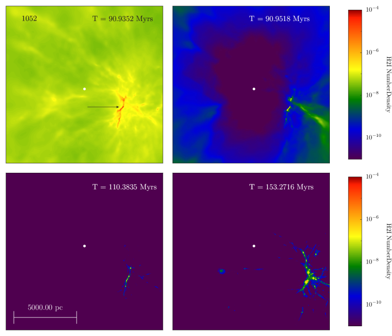
Figure 1.— The neutral H2I density evolution shown, in projection, for simulation 1052 for illustration. The source is switched on at z = 32, which corresponds to T = 90.9352 Myrs - top left panel.The source is represented by the filled white circle. The arrow in the top left panel points at the center of maximum density of the collapsing halo of interest. As the photons from the source travel outwards they dissociate $\rm{H_{2}}$. The top right hand panel shows the H2I number density approximately $10^{5}$ yrs later. At this stage the density of $\rm{H_{2}}$ has been reduced by several orders of magnitude. As the time evolution continues the flux from the source keeps the $\rm{H_{2}}$ levels strongly suppressed. However, as the simulation proceeds the gravitational collapse and subsequent increase in density of atomic hydrogen enables the formation rate of $\rm{H_{2}}$ in the collapsing structure to out-pace that of the dissociating background. The $\rm{H_{2}}$ formation rate is driven by the reaction H^- + H $\rightarrow$ $\rm{H_{2}}$ + e. In the bottom right panel the growth of the halo and the increased density of $\rm{H_{2}}$, in the face of a dissociating source, is clearly visible.

2.1. Halo Selection

Only a single halo is used in this study that has a mass $M\simeq 10^{6}M_{\odot}$ at $z=30$ and grows to $M\simeq 6\times 10^{7}M_{\odot}$ by $z=21$. The simulation is rerun multiple times with different radiation parameters, as detailed in Table 1 but the initial conditions are unchanged for each run. The halo was originally identified in a previous study (Regan et al., 2014). It corresponds to a very rare peak in the linearly extrapolated density field. In terms of the rms fluctuation amplitude, $\nu=4.2$, where $\nu$ is defined as

$$\nu={\delta_{c}\over\sigma(M)D(z)}$$ (1)

where $\delta_{c}\approx 1.686$ is the threshold over-density for a spherical collapse (Gunn & Gott, 1972), $D(z)$ is the growth factor and $\sigma(M)$ is the mass fluctuation inside a halo of mass M. The mass fluctuation is given by

$$\sigma^{2}(M)=\int{k^{2}\over{2\pi^{2}}}P(k)W(kR)dk$$ (2)

where the integral is over the wavenumber $k$, $P(k)$ is the power spectrum and $W(kR)$ is the top hat window function. In this context $\nu=4.2$ corresponds to a very rare halo. A $\nu=4.2$ peak corresponds to a host halo with a mass of $\rm{M}\approx 1\times 10^{12}$ $\rm{M_{\odot}}~{}$at $\rm{z\sim 6}$. It was convenient in this case to look for a halo collapsing early, and rapidly, to alleviate the computational demands set by the radiative transfer module. In addition, the very high redshift of the collapse $(z\sim 20-30)$ in this case strengthens our assumptions of a negligible global LW background as well as the absence of metals and dust. Furthermore, these rare density peaks are the most likely progenitors of the $z\gtrsim 6$ quasar hosts (e.g. Costa et al., 2014).

2.2. Radiative Particles

The simulations conducted in this paper used a massless radiation source particle. We added this feature to the stable version of the Enzo code. In order to complete the modification the new particle type was coupled together with the radiative transfer module so that the particle became a source particle capable of producing a LW flux of a given flux density. The active particle is not created on the fly as it does not result from the collapse of gas or any other physical mechanism. The code is stopped at a predefined point in time, the particle’s coordinates are supplied and the particle is inserted into the code using a simple input file. The particle data is read by the code and is recognised as a radiation source particle. We choose the current approach as it gives us maximum flexibility in terms of where we put the source particle relative to the halo of interest. We now describe the radiative transfer setup used in this work.

2.3. Radiative Transfer Setup

The $\rm{H_{2}}$ dissociating radiation emitted by the massless source particle is propagated with adaptive ray tracing (Abel & Wandelt, 2002; Wise & Abel, 2011) that is based on the HEALPix framework (Górski et al., 2005). The radiation field is evolved at every hydrodynamical timestep of the finest AMR level. The $\rm{H_{2}}$ dissociation that occurs at each timestep couples to the hydrodynamical component self-consistently. The photons travel at infinite speed through the simulation at each timestep with the photons halted when one of the following conditions is met:

1. The photon travels 0.7 times the simulation box length

2. The photon flux is almost fully absorbed ($>99.9\%$) in a single cell.

Photons are therefore traced, at each hydrodynamic timestep, through the entire region of interest. The instant light propagation is motivated by the fact that the dynamical time is long compared to the light propagation timescale.

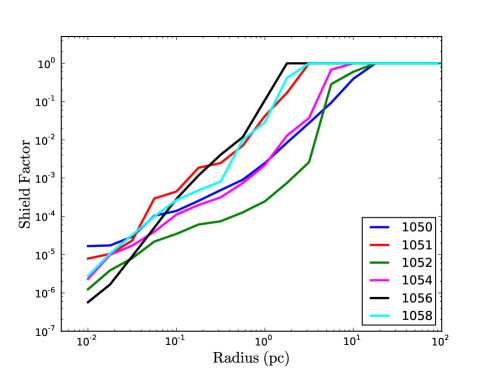
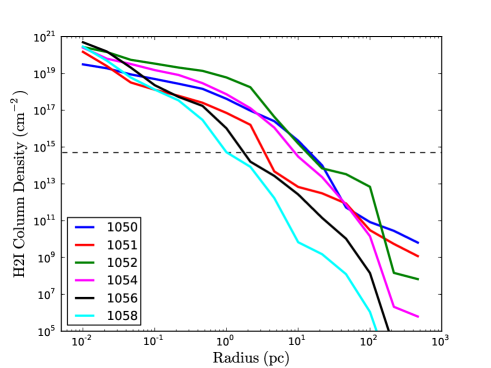
Figure 2.— The left panel shows the shielding factor calculated at the moment each simulation reaches the highest level of refinement (18). To calculate the shielding factor 500 sightlines are drawn from the source to an area surrounding the point of maximum density. The average over all sightlines is then used. The shielding factor is determined using the formula given in WG11 (and reproduced here as equation 3) which depends both on the column density of the gas and its temperature. The right hand panel shows the $\rm{H_{2}}$ column density found along the same sightlines as the shielding factor. The dashed line indicates the column density above which the $\rm{H_{2}}$ is assumed to be optically thick (see eqn 3). Note that the HI column densities would be a factor of approximately $\sim 10^{3}$ higher in the central regions than the $\rm{H_{2}}$ column densities shown here.

Photons dissociate $\rm{H_{2}}$ as they travel outwards (see Figure 1) from the source. We use an average cross-section for $\rm{H_{2}}$ dissociation of $3.71\times 10^{-18}$ cm² to calculate the dissociation rate as photons pass through the gas. The medium through which the photons travel is assumed to be optically thin below a $\rm{H_{2}}$ column density of $5\times\rm{10^{14}\ cm^{-2}}$. Above this limit the self-shielding approximation taken from Wolcott-Green et al. (2011), hereafter WG11, is used. The shielding approximation is based on earlier work by Draine & Bertoldi (1996). In the high column density regime $\rm{H_{2}}$ is assumed to be optically thick and the dissociation rate is calculated using a fitting function. The fitting function is given by

$$\begin{split}\rm{Shield\ (N_{H_{2}})}\ &={0.965\over(1+X/b_{5})^{\alpha}}\\ &+{0.035\over(1+X)^{0.5}}\times\rm{exp}[-8.5\times 10^{-4}(1+X)^{0.5}]\end{split}$$ (3)

where $\alpha$ is set to be 1.1 in this study, $X\equiv N_{H_{2}}/(5\times 10^{14}\ \rm{cm^{-2}})$, $\rm{b_{5}\equiv b/(10^{5}\ cm\ s^{-1})}$ and b is the usual Doppler parameter in this case. This fitting function is used to accurately account for the self-shielding of $\rm{H_{2}}$ from dissociating radiation which occurs at column densities above $5\times 10^{14}\ \rm{cm^{-2}}$; see WG11 for more details. The use of a self-shielding approximation is required in simulations using radiative transfer techniques at these scales so as to make the simulation computationally viable with the expected errors from using such fits expected to be small (Draine & Bertoldi, 1996).
The massless source particles used in our simulations are all monochromatic, emitting radiation at the center of the Lyman-Werner band only, the energy of the photons is set to be $12.8$ eV $(\lambda=96.9\ \rm{nm})$ in all cases. The details of each simulation is given in Table 1. The name of each simulation gives the source flux, for example simulation 1052 has a source flux of $10^{52}$ photons per second.

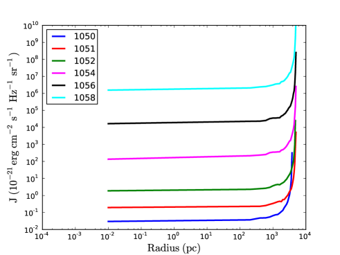
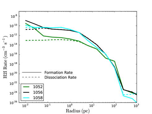
Figure 3.— The left hand panel shows the value of the flux, J, calculated along the same 500 lines of sight from the source to the center of maximum density as was done for the shielding factor calculation. The value of J varies from less than $1\times 10^{-1}\ J_{21}$ to greater than $1\times 10^{6}\ J_{21}$ within 10 parsecs of the center. J is calculated in this case at the point where the simulation reaches the maximum refinement level. The right hand panel shows both the $\rm{H_{2}}$ formation rate and the $\rm{H_{2}}$ dissociation rate computed using the same 500 sightlines and averaging over them. The solid lines are the formation rates while the dashed lines are the dissociation rates. The $\rm{H_{2}}$ formation rate overwhelms the $\rm{H_{2}}$ dissociation rate in the central regions. Only the results from simulations 1052, 1056 and 1058 are shown for clarity.

3. Flux to Background Intensity Relation

In all direct collapse simulations to date, in which a radiation module has been included, the authors have used a homogeneous and isotropic background UV flux to capture the effects of sources capable of dissociating $\rm{H_{2}}$. The radiation flux amplitude, $J$, is usually measured in units of $J_{21}=\$$\rm{10^{-21}\ erg\ cm^{-2}\ s^{-1}\ Hz^{-1}\ sr^{-1}}$. This represents the intrinsic brightness or intensity of a source which is assumed to be constant at all points in space. The spectral flux at each point in space is then easily recovered by integrating over all angles. For the case of a stellar source the result of the integration is $\pi$ (see e.g. Bradt, 2008, page 211) while for the case of an isotropic field the result of the integration is 4$\pi$.
In our simulations we neglect any contribution from background sources and calculate only the intensity from a single anisotropic close-by source of high intensity. In Table 2 we show the flux of the source in each of our simulations. The source is placed at the same point in each simulation. Thus calculating the observed flux at the point of maximum density, when the source is switched on, is straightforward. In this case $J$ is given by:

$$J={\mathrm{Photons\ emitted\ per\ second}\times h\over 4\pi^{2}r^{2}}$$ (4)

where h is Planck’s constant and $r$ is the distance from the radiation source to the point of maximum density under the assumption that the medium is optically thin at all points, the second factor of $\pi$ in the denominator accounts for the solid angle. Furthermore, we have used the frequency value at the center of the LW band only in the above conversion with the effect that the frequency, $\nu$, cancels out above and below the line. The value of $J$ is shown in column 4 of Table 2 in units of $J_{21}$. The values in Table 2 are calculated at the time at which the source turns on. An effective stellar temperature of $T_{\rm eff}\sim 50000$ K is required to produce a spectrum which peaks in the LW bands. This effective temperature is typical of massive stars with masses in excess of $M_{*}\gtrsim 50$ $\rm{M_{\odot}}$.

4. Results

Table 1 shows the values of a range of physical quantities when the refinement level reaches the maximum refinement level allowed in our simulation, which is 18 in this case. The maximum comoving spatial resolution reached in our simulations is $\sim 1.5\times 10^{-2}\ \rm{h^{-1}\ pc}$, while the maximum proper resolution reached near the end of each realization is $\sim 2.5\times 10^{-3}\ \rm{h^{-1}\ pc}$. The results show a variation in the time of collapse of the object due to the source flux amplitude. We begin by examining the quantities in each simulation that affect the ability of the gas to shield against the dissociating radiation, doing so allows us to determine what level of flux is required to first of all dissociate $\rm{H_{2}}$ and then to restrict its abundance. Throughout the following sections we refer to the core of the simulation as the region within 1 parsec of the point of maximum density and to the envelope as the region surrounding the core extending to approximately 30 parsecs.

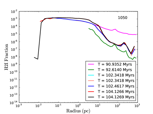
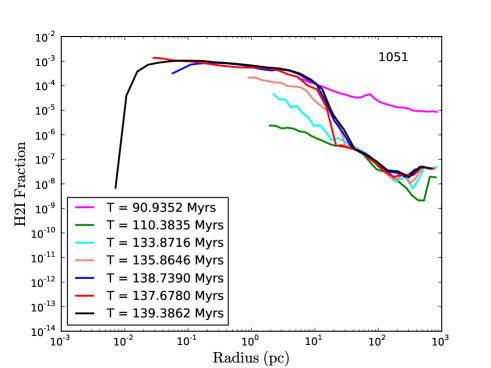
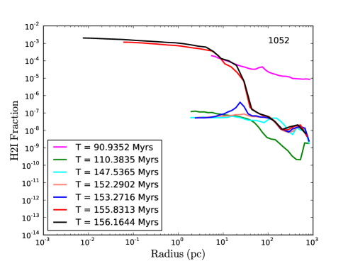
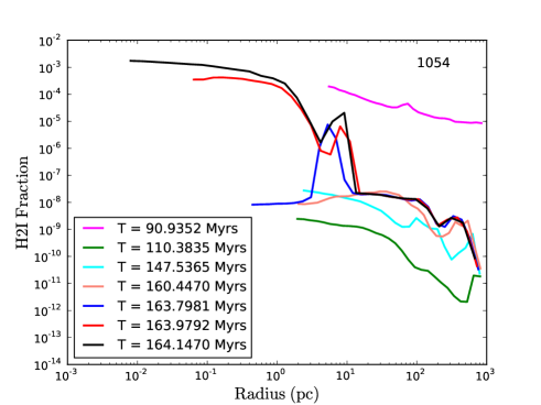
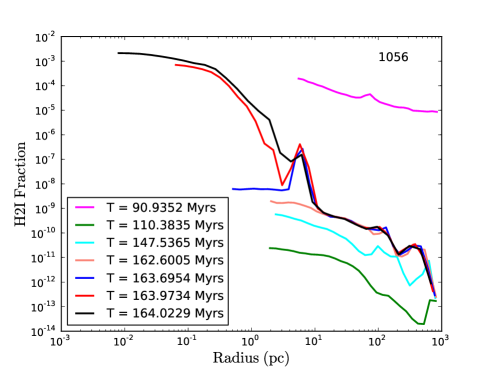
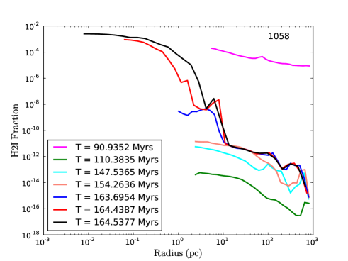
Figure 4.— Shown are the timeseries plots of the $\rm{H_{2}}$ fraction is each of the simulations listed in Table 1. The source is switched on at 90.9352 Myrs (z = 32), at that point the $\rm{H_{2}}$ Fraction in the halo of interest is between $10^{-3}$ and $10^{-4}$. The $\rm{H_{2}}$ molecules in the halo are quickly dissociated and their density reduced by several orders of magnitude. The $\rm{H_{2}}$ formation rate however increases as the density of HI builds up and eventually overcomes the dissociation rate. The halos in simulations 1050 and 1051 never reach atomic cooling status and they are always dominated by $\rm{H_{2}}$ cooling. In each of the other halos the fraction of $\rm{H_{2}}$ is suppressed sufficiently such that the halos cool predominantly via neutral hydrogen but note that $\rm{H_{2}}$ forms readily in the core.

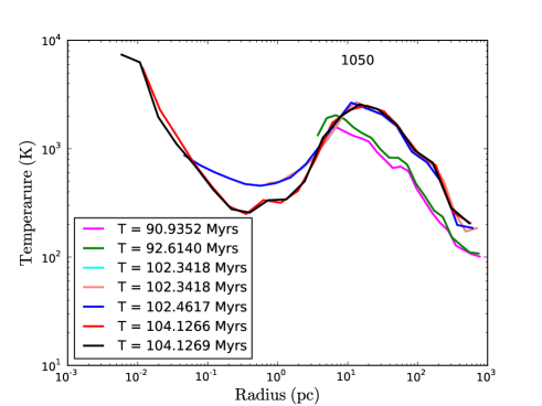
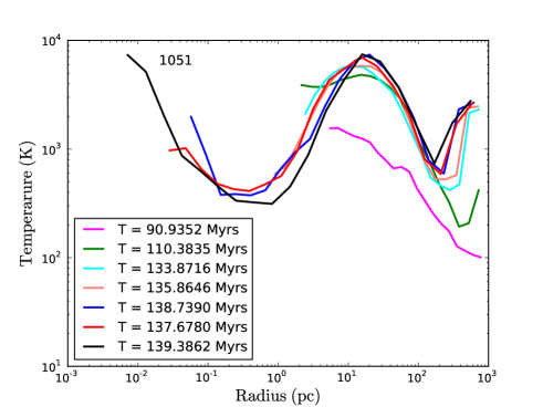
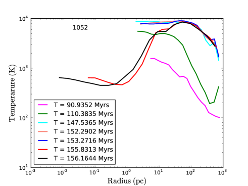
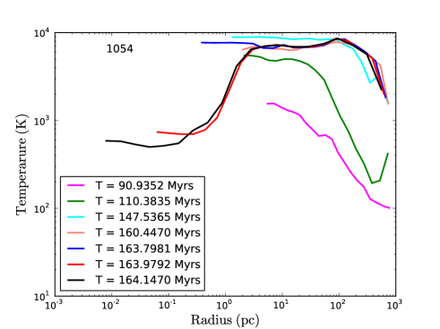
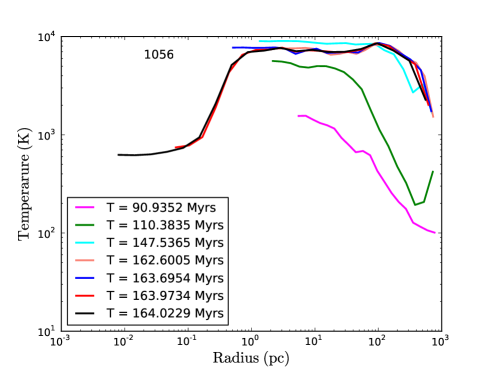
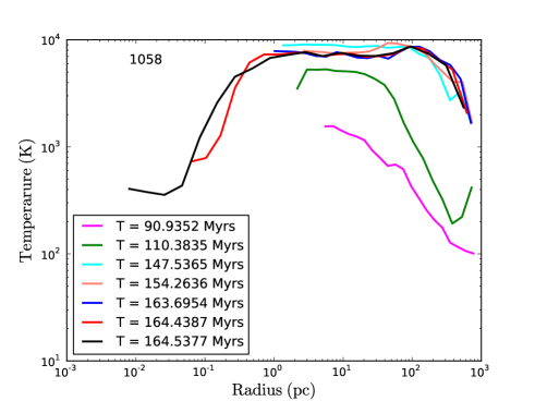
Figure 5.— The temperature timeseries for the same times and simulations as the $\rm{H_{2}}$ fraction timeseries plots (Figure 4). The temperature is initially close to $T\approx 10^{3}\ \rm K$ with cooling by $\rm{H_{2}}$ prominent. The halo in simulation 1050 is able to cool via $\rm{H_{2}}$ despite the dissociating source and quickly collapses, the halo in 1051 is more resistant and must initially cool via HI (although its virial temperature is $T_{\rm vir}\ll 10^{4}\ \rm K$). Nonetheless the halo in 1051 is able to form $\rm{H_{2}}$ in large quantities once the HI density increases. This then triggers a collapse via $\rm{H_{2}}$ cooling. The other four halos experience stronger dissociating fluxes and the temperature remains at $T\sim 10^{4}$K for a significant time. Ultimately $\rm{H_{2}}$ is formed in the core in each case causing a sudden drop in the central temperature.

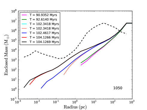
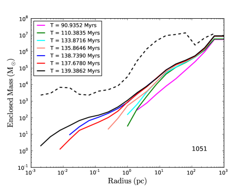
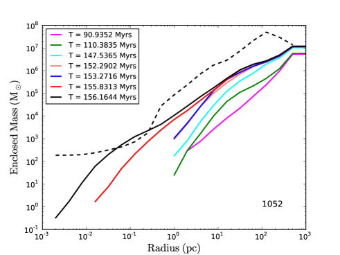
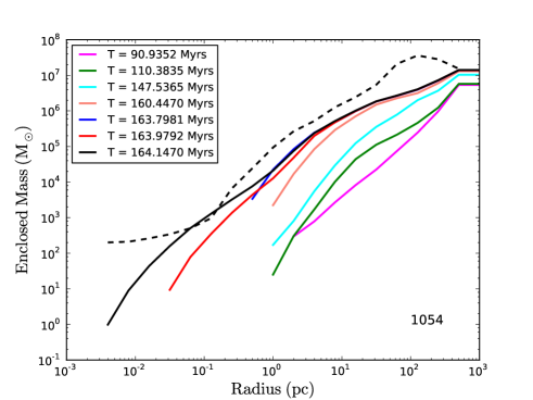
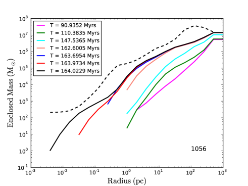
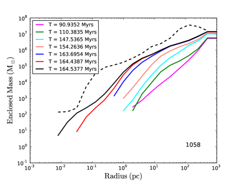
Figure 6.— The enclosed mass for each simulation with the same output times as Figure 4 and Figure 5. The solid curves are the enclosed cell mass values while the dashed lines give the Jeans mass at the final output time at the corresponding radius.

4.1. $\rm{H_{2}}$ Self-Shielding

The left panel of Figure 2 shows the shielding factor computed by averaging over 500 lines of sight between the source and the area surrounding the point of maximum density. All sight sightlines travel the same distance. In each simulation the shield factor outside of approximately 30 parsecs (outside the envelope) of the collapsing halo is 1.0, indicating that the medium is optically thin outside of this region. Within 30 parsecs the shielding factor quickly decreases to values between $10^{-5}$ and $10^{-6}$ approximately. There is also a trend for higher fluxes to enter the optically thick regime at distances closer to the center of the maximum density as expected, e.g. simulation 1058 only enters the optically thick regime at approximately a distance of 3 parsecs. The shielding factor also displays significant scatter between simulations, this is expected given the shielding factor (see equation 3) is a function of both the column density and the temperature along a given sightline.
The right hand panel of Figure 2 shows the $\rm{H_{2}}$ column density computed along the same 500 sightlines and also averaged. Similar to the shielding factor there is a trend towards higher fluxes showing a smaller $\rm{H_{2}}$ column density as expected. The horizontal dashed line in the figure at $\rm{5\times 10^{14}\ cm^{-2}}$ shows the point at which the medium is no longer assumed to be optically thin and where $\rm{H_{2}}$ self-shielding begins (Draine & Bertoldi, 1996; Wolcott-Green et al., 2011). The maximum molecular hydrogen column density reached at the very center of the collapsing halo is between $\rm{1\times 10^{19}\ cm^{-2}\ and\ 1\times 10^{21}\ cm^{-2}}$.
The left hand panel of Figure 3 shows the value of $J$ along the same 500 lines of sight connecting the source and the point of highest density. The values are computed at the end of the simulation - as the simulation reaches the point of maximum refinement. Within 100 parsecs the value of $J$ varies from $J\sim 10^{-2}\ J_{21}$ to $J\sim 10^{6}\ J_{21}$. For reference the global background at this redshift is expected to be $\rm{J_{LW\ Global}\lesssim 1.0\ \times\ }J_{21}$ (e.g. Dijkstra et al., 2008).
Finally, the right hand panel of Figure 3 shows the formation rate and the dissociation rate of $\rm{H_{2}}$ for three selected simulations (1052, 1056 & 1058) at the highest refinement level. The solid line is each plot represents the $\rm{H_{2}}$ formation rate while the dashed line of the same color represents the dissociation rate. The formation rate is calculated using the fitting formulae as used in the Enzo code (Abel et al., 1997) while the dissociation rate is calculated self-consistently by the radiative transfer module (see §2.3). For simulation 1052, we see up until approximately 100 parsecs from the center of maximum density that the dissociation rate matches perfectly the formation rate and no new $\rm{H_{2}}$ can be created (further from the halo the dissociation rate exceeds the formation rate). However, within 100 parsecs the formation rate for simulation 1052 overwhelms the dissociation rate and $\rm{H_{2}}$ can form. A similar characteristic is shown for both simulations 1056 and 1058. However, in the case of 1056 and 1058 the formation rate is only able to exceed the dissociation rate much closer to the center of the halo, at approximately 5 parsec and 2 parsec distances, respectively. In all cases this indicates that $\rm{H_{2}}$ is readily formed in the core of the halo, even in the presence of extremely strong fluxes, due to the increase in the $\rm{H_{2}}$ formation rate compared to the dissociation rate.

4.2. Physical Characteristics of the Illuminated Halo

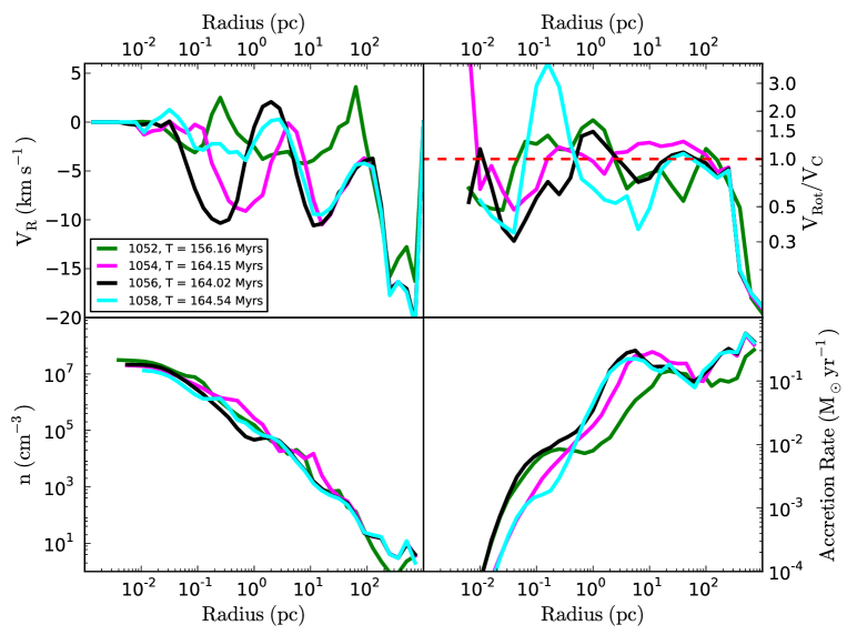
Figure 7.— All halos that reach atomic cooling status are shown. The plots are at the time each simulation reaches the maximum refinement level. The bottom left panel shows the gas number density, $n$, plotted as a function of radius. The top left panel shows the radial velocity, $V_{R}$, as a function of radius. The top right panel shows the ratio of the rotational velocity to the circular velocity, $V_{Rot}/V_{C}$, as a function of radius. The bottom right panel shows the mass accretion rate, $\dot{M}$, as a function of radius at the final output time.

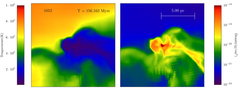
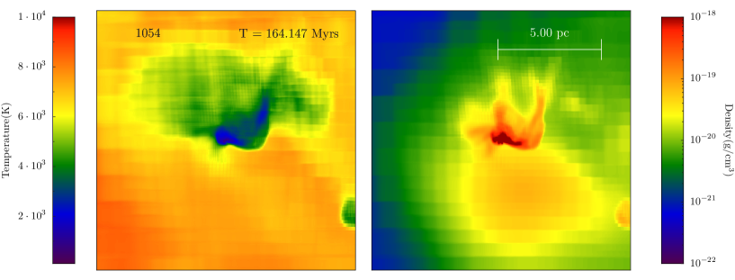
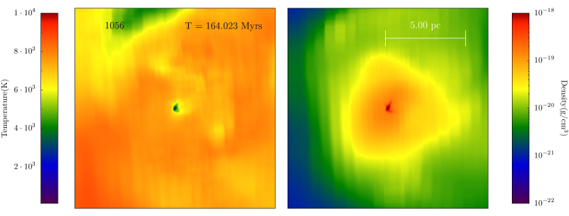
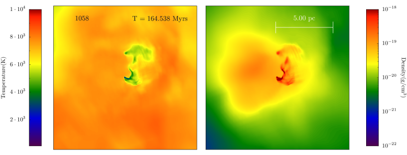
Figure 8.— Each halo is shown in projection as it reaches the highest refinement level. The projection in each case is made along the angular momentum vector. The left panel of each row shows the temperature across approximately 10 parsecs. The right panel in each row shows the density in the same region. The projections are shown only for the fours halos which reach the atomic cooling threshold. The spatial scales of all panels are identical.

4.2.1 Time Series Analysis

We begin by looking at a time series analysis of the collapsing halos when they are subjected to different $\rm{H_{2}}$ dissociating fluxes. In Figure 4 we show the $\rm{H_{2}}$ fraction for each of our simulations, where each panel is for a different source flux. We use radial profiling to examine the quantities. Radial profiling allows us to best determine the properties of the gas surrounding the core and envelope. While the radiation is anisotropic and thus comes from a preferred direction, the dominant gravitational forces acting during the collapse do not have a preferred direction and so in this case radial profiling best captures the state of the gas for all but the very earliest stages after the source is switched on.
In each case we start at the time at which the source was switched on (T = 90.9352 Myrs, corresponding to $z=32$). Each simulation was run until the maximum refinement level was reached. What is clearly noticeable from each simulation is that initially the $\rm{H_{2}}$ fraction decreases by a large factor, with larger drops for larger flux amplitudes as expected. For simulations 1050 and 1051 the decrease in the $\rm{H_{2}}$ fraction is quickly recovered. Simulation 1050 in particular reaches $\rm{H_{2}}$ values comparable to its initial value within 10 Myrs and subsequently collapses to form a minihalo - capable of forming population III stars (e.g. Abel et al., 2002). Similarly simulation 1051 displays a similar trend, albeit the collapse to a minihalo takes longer and is significantly delayed. Both halos also display a strong decrease in $\rm{H_{2}}$ at the very center of the halo, as has been seen before in simulations of population III star formation (e.g. Turk et al., 2012). This is caused by the collisional dissociation of $\rm{H_{2}}$ as gas rapidly flows to the center of the newly formed potential.
Simulations 1052, 1054, 1056 and 1058 all experience a strong dissociating flux. As a result the $\rm{H_{2}}$ fraction is strongly suppressed initially. For each of these fluxes the collapse takes place approximately 60 Myrs after the source switched on, equivalent to a delay of approximately 50 Myrs from the case it which no flux exists. Within the central 10 - 40 parsecs the fraction of $\rm{H_{2}}$ increases rapidly due to the formation rate of $\rm{H_{2}}$ exceeding its dissociation rate (see Figure 2 and Figure 3). By the end of each simulation the $\rm{H_{2}}$ fraction in the core of the halo (within $\sim 1$ parsec) has returned to its equilibrium value of $1\times 10^{-3}$.
In Figure 5 we plot the temperature profile for each of our simulations. Simulation 1050 is almost completely unaffected by the dissociating flux, the temperature remains close to $T=10^{3}\ \rm K$ for most of the simulation. As the HI density grows the formation of $\rm{H_{2}}$ is enhanced at around 10 parsec distances and the temperature decreases to $T\sim 500\ \rm K$. At the very end of the simulation and deep within the core ($\rm{R\lesssim 1}$ parsec) where $\rm{H_{2}}$ is collisionally dissociated we do see the temperature significantly exceeding $T=10^{3}\ \rm K$. Simulation 1051 behaves similarly, although the stronger flux, compared to simulation 1050, means that the temperature in the halo increases to closer to $T=10^{4}\ \rm K$, in fact reaching values around $T\sim 8000\ \rm K$ at approximately 10 parsecs. At this point however, the rapid formation of $\rm{H_{2}}$ drives the temperature back down to closer to $T\sim 500\ \rm K$ similar to the 1050 case.
The atomic halos (1052, 1054, 1056, 1058) instead show a rather different behavior. The initial strong suppression of $\rm{H_{2}}$ means that the temperature quickly rises. Within approximately 20 - 30 Myrs the temperature of the gas has reached $T\sim 10^{4}\ \rm K$. The main coolant is now HI and the virial temperature of the halo quickly exceeds $T\gtrsim 10^{4}\ \rm K$. The gas remains at $T_{\rm{Vir}}\sim 10^{4}\ \rm K$ as the halo begins its collapse. However, within $\sim$ 10 parsecs of the center, the $\rm{H_{2}}$ fraction (see Figure 4) is able to grow considerably. The presence of $\rm{H_{2}}$ has a dramatic effect on the gas temperature enabling cooling back down to $T\sim 1000\ \rm K$. This is the case in the centers of each of the atomic halo simulations.
Finally, in Figure 6 we show the enclosed gas mass as a function of radius from the point of maximum density. The solid line in each panel is the enclosed mass. For reference the Jeans Mass, at that radius, is plotted (dashed black line) for the final output time. Once the Jeans mass is exceeded the gas becomes gravitationally unstable to collapse. Both simulations 1050 and 1051 fail to exceed the Jeans threshold at any radius (although 1050 does show signs of instability as expected close to $M\sim 10^{3}$ $\rm{M_{\odot}}$). In both cases the gas is collapsing via $\rm{H_{2}}$ cooling and has yet to form a self-gravitating clump by the end of the simulation. However, both are expected to collapse within a short time as the clump accretes mass and the enclosed mass increases. The minimum of the Jeans mass is at $M\sim 10^{3}$ $\rm{M_{\odot}}~{}$in both cases and it is at this radius that we expect the first gravitational instability to appear and subsequently fragment and form Pop III stars (Turk et al., 2009; Clark et al., 2011; Greif et al., 2011, 2012). The atomic mass halos (1052, 1054, 1056, 1058) show qualitatively similar behavior but important differences exist. Simulations 1052 and 1054 both display gravitational instability at $M\sim 10^{3}$ $\rm{M_{\odot}}$, this is because the mass accretion rate onto these halos is higher than in both 1050 and 1051 and hence more mass has accumulated at each radius. The enclosed mass exceeds the Jeans value at approximately $\rm{M\sim 10^{3}}$ $\rm{M_{\odot}}$. The reason for this is because they are both able to rapidly form $\rm{H_{2}}$ within 10 parsecs (reaching fractions of approximately $1\times 10^{-5}$ at 10 parsecs), this increase in $\rm{H_{2}}$, and corresponding decrease in temperature, drive the Jeans value downward and the predominantly molecular hydrogen clump becomes self-gravitating. However, in both 1056 and 1058, the $\rm{H_{2}}$ fraction does not reach the level of $1\times 10^{-5}$ until closer to 1 parsec due to the higher dissociation rate. As a result the formation of a smaller clump is suppressed in simulations 1056 and 1058 although it is not completely negated as $\rm{H_{2}}$ still readily forms within the self-shielded core (see right hand panel of Figure 3).
It is also worth noting that in simulations 1054, 1056 and 1058 the enclosed mass profile displays a clear plateau at $M\gtrsim 10^{5}$ $\rm{M_{\odot}}$. The plateau becomes more pronounced as the source flux increases, with a clean example emerging in simulation 1058. The plateau is the signature of a disk-like structure forming similar to what has been seen in atomic only simulations (e.g. Regan & Haehnelt, 2009b; Regan et al., 2014). The collapse at the center of the halo and the subsequent decrease in the timestep means that the evolution of the envelope containing $M\sim 10^{5}$ $\rm{M_{\odot}}~{}$is effectively frozen out. Tracking the evolution of the envelope from this point onwards is therefore very difficult due to its relatively long dynamical time compared to the dynamical time of the mass at the center of the collapse. Nonetheless, it seems likely that this larger mass will collapse with a mass of close to $M\sim 10^{5}$ $\rm{M_{\odot}}~{}$in all three cases (1054, 1056, 1058) with the possible exception of simulation 1054 where a smaller mass star ($M\sim 10^{3}$ $\rm{M_{\odot}}~{}$) may initially form due to the larger $\rm{H_{2}}$ fraction in this case.

4.2.2 Comparison at Maximum Refinement

In Figure 7 we have over-plotted several physical characteristics from the atomic halo (1052, 1054, 1056 and 1058) outputs when the simulation reaches the maximum level of refinement, which is 18 in this case. In the bottom left panel we plot the gas number density (hereafter referred to simply as the number density, unless explicitly stated otherwise) as a function of radius. The maximum number density reached in each simulation is $n\sim 3\times 10^{7}\ \rm cm^{-3}$. As we see each simulation asymptotes towards a cored profile in the inner regions of the plot. This core is due to the formation of a small disk at the very center of the collapsing halo - due to the formation of $\rm{H_{2}}$ and its subsequent collapse.
In the top left panel we have plotted the radial velocity against the radius. The radial velocity shows a very strong inflow at a distance of a few hundred parsecs. This is where the gas is flowing rapidly into the halo and the point at which shock heating occurs (see Figure 5). Simulations 1054, 1056 and 1058 all show strong radial inflows at distances between a few parsecs and approximately 100 parsecs. In particular, there is a noticeable peak in the radial velocities of all four simulations at approximately 20 parsecs and another peak between 0.1 and 1.0 parsecs. In the case of simulations 1054 and 1056 this is due to the formation of an inner collapsing object with mass of $\rm{M}\sim 10^{3}$ $\rm{M_{\odot}}~{}$(the core) and an outer collapsing object (the envelope) with a of mass $\rm{M}\sim 10^{5}$ $\rm{M_{\odot}}$. In simulation 1058 the radial inflow is dominant at approximately 20 parsecs but with only a relatively weak radial inflow at the smaller collapsing radius. This is because of the relative lack of $\rm{H_{2}}$ in the core in this simulation and indicates that only the envelope will collapse with a mass of close to $M\sim 10^{5}$$\rm{M_{\odot}}$.
In the top right panel we plot the ratio of the rotational velocity against the Keplerian (circular) velocity. The rotational velocity is calculated by computing the inertia tensor and then using the angular momentum vector to find the rotational velocity around the principal axis. This approach is detailed in Regan & Haehnelt (2009b) to which we direct the reader for further information. A value of $\rm{V_{Rot}/V_{C}}>1$ indicates that the gas is rotationally supported (red dashed line). The rotational support ratio shows qualitatively the same behavior as the radial velocity plot. There is a peak in rotational support at a distance of approximately 20 parsecs in each case and rotational support is achieved in all cases at this point. Simulations 1052 and 1056 achieve a peak in rotational support again inside 1 parsec consistent with the formation of a $\rm{H_{2}}$ clump at that radius. Simulation 1054 maintains a more consistent, rotationally supported, profile into the core. Simulation 1058 displays rotational support between approximately 10 parsecs and 100 parsecs, the ratio then dips below 1.0 inside 10 parsecs and apart from a spike at 0.2 parsecs due to a spike in the $\rm{H_{2}}$ fraction and associated temperature decrease remains below 1.0 at all radii inside 10 parsecs. The inner core of simulation 1058 is therefore not rotationally supported. The bottom panel in Figure 8 shows the rather unrelaxed nature of the inner core in this simulation and provides an explanation for the anomalous behavior at small radii in this case.
Finally, in the bottom right panel we plot the mass accretion rate against the radius. The accretion rate is the instantaneous accretion rate calculated by taking the difference between two outputs at the end of the simulation. The accretion rate in all four cases shows a noticeable plateau between a radius of a few parsecs and about 30 parsecs, this is due to the collapsing $\rm{M\sim 10^{5}}$ $\rm{M_{\odot}}~{}$clump forming at this radius and accreting mass at a rate of $\sim 0.25$ $\rm{M_{\odot}}~{}$$\rm{yr^{-1}}$. This accretion rate is consistent with that predicted by Inayoshi et al. (2014) and Schleicher et al. (2013) for the formation of a supermassive star or possibly a quasi-star depending on the long term evolution of the acretion rate. Also worth noting is that simulation 1052 plateaus again at a radius between approximately 0.05 and 1 parsecs, this plateau is due to accretion onto the $\rm{M\sim 10^{3}}$ $\rm{M_{\odot}}~{}$clump collapsing due to $\rm{H_{2}}$ cooling. This plateau is not as well defined in simulations 1054, 1056 and 1058 due to the higher dissociation rate.
In Figure 8 we show density weighted projections of both the temperature and density for each of the atomic cooling halos (1052, 1054, 1056 and 1058) at the time the simulation first reaches the maximum refinement level. The projection is made along the angular momentum axis in each case and so is specific to each halo. This along with the fact that the time at which the simulation reaches the maximum refinement level is different in each case means that the morphology of each halo is significantly different in all cases. In each simulation the central object forms in the center of the cold, $\rm{H_{2}}$ cooled, gas. What is immediately clear is that the fraction of cold gas available in simulation 1052 is significantly greater than in the 1056 and 1058. In both 1056 and 1058 it is clear that only a very small fraction of the gas is collapsing due to the formation of $\rm{H_{2}}$. Furthermore, both 1056 and 1058 show the envelope (with a diameter of approximately 10 - 20 parsecs) surrounding the core. Simulation 1054 represents an intermediate case with a well defined envelope and a substantial fraction of $\rm{H_{2}}$ within the core. The radiation in the case of 1054 is not strong enough to penetrate all the way to the center meaning a larger fraction of $\rm{H_{2}}$ is able to form.

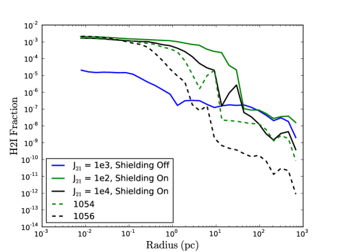
Figure 9.— This figure compares the $\rm{H_{2}}$ fraction when the simulation is run using different prescriptions for the radiation. In the first three cases (blue, green & black solid lines) the radiation is isotropic with different intensities. Furthermore, the blue line contains no self-shielding, the green and black solid lines do but the radiation intensities are different. The dashed green and dashed black lines are the lines from simulations 1054 and 1056 for comparison.

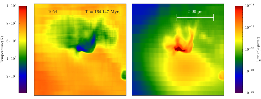
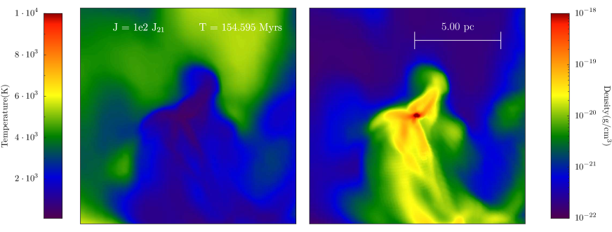
Figure 10.— The top row is the same as the second row in Figure 8, it is the projection of the 1054 simulation at the highest refinement level made along the angular momentum vector. The bottom row shows the projection for the $\rm{J=1\times 10^{2}\ J_{21}}$ isotropic radiation case with self shielding. The left panel of each row shows the temperature across approximately 10 parsecs. The right panel in each row shows the density in the same region. The spatial scales of both panels are identical.

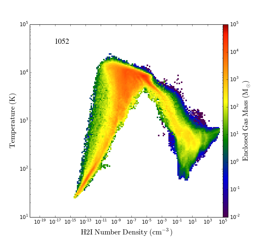
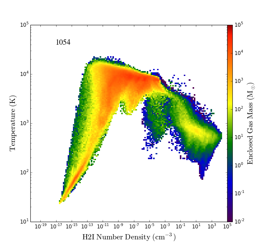
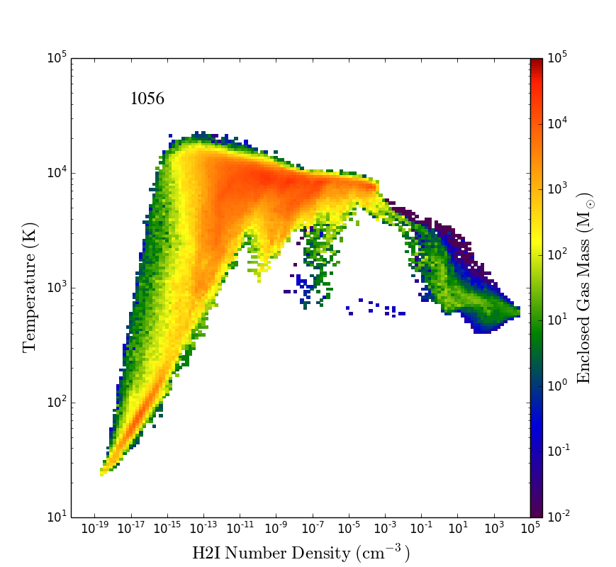
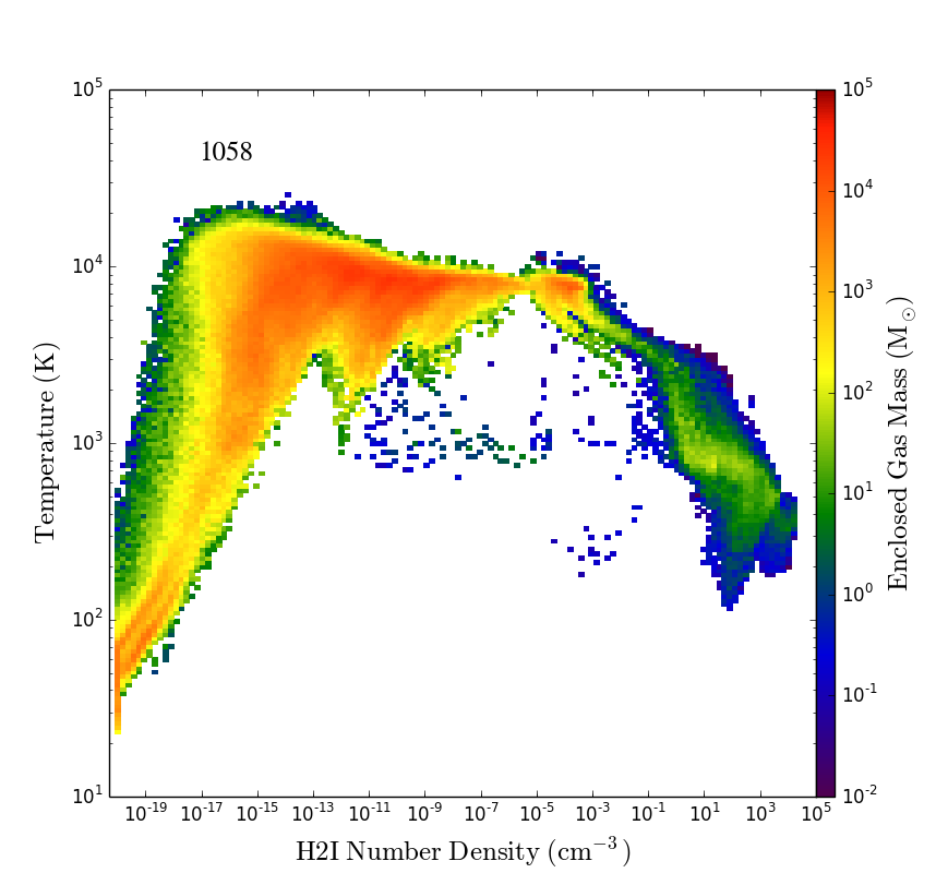
Figure 11.— A Phase Space plot for each of the atomic cooling halos with $\rm{H_{2}}$ Number Density (x-axis) plotted against Temperature (y-axis). The pixels are colour coded according to the enclosed gas mass. In the top left panel the halo reaches atomic cooling status at its outer regions but within a few tens of parsecs the $\rm{H_{2}}$ fraction increases rapidly and a significant fraction of the gas is able to cool to below $10^{3}$ K. As the flux increases in each panel the amount of gas than is able to stay at $\sim 10^{4}$ K increases rapidly. In the highest flux simulation (bottom right panel) only a small fraction of the gas cools to below $10^{3}$ K.

5. Comparison against isotropic radiation field

Finally, we wish to compare, as best as possible, the effect of an isotropic radiation field versus an anisotropic radiation field. We make the comparisons in Figure 9 and Figure 10. As done throughout this paper outputs are compared when the simulation reaches the highest refinement level. Fundamentally, the isotropic field means that each cell “feels” the same radiation whereas with the anisotropic source the intensity varies as $1/r^{2}$ in the optically thin regions and according to equation 3 in the optically thick regions. We ran a number of simulations, with an isotropic background and using the same halo as was used throughout this study in order to compare the results. Furthermore, we included a local approximation to calculate the $\rm{H_{2}}$ column density in each cell and used that value to estimate the self-shielding factor due to $\rm{H_{2}}$. In order to calculate the local estimate of the $\rm{H_{2}}$ column density we use the ’Sobolev-like’ method (Sobolev, 1957; Gnedin et al., 2009) to estimate the column density. In this case the characteristic length is obtained from

$$L_{\rm{Sob}}\equiv{\rho\over|\nabla\rho|}$$ (5)

where $\rho$ is the gas density. This particular method has been shown by WG11 to be particularly accurate in estimating the column density locally. The self-shielding approximation is then implemented in the same fashion as in the ray-tracing simulations, i.e. using equation 3.
The solid blue line in Figure 9 uses an isotropic background radiation field with $\rm{J=1\times 10^{3}~{}J_{21}}$ and no $\rm{H_{2}}$ self-shielding. The solid green line uses a lower intensity field with $\rm{J=1\times 10^{2}~{}J_{21}}$ but this time $\rm{H_{2}}$ self-shielding is included. The solid black line uses a higher intensity field with $\rm{J=1\times 10^{4}~{}J_{21}}$ and with $\rm{H_{2}}$ self-shielding included. For comparison the results from simulations 1054 (dashed green line) and 1056 (dashed black line) are also included. The dashed lines should therefore be compared with the solid lines of the same color. In all cases the radiation field is switched on at a redshift of $z=32$. We specifically picked isotropic backgrounds with intensities of $\rm{J=1\times 10^{2}~{}J_{21}}$ and $\rm{J=1\times 10^{4}~{}J_{21}}$ so as to match closely the values simulations 1054 and 1056 reach at the point of maximum density (i.e approximately 3 kpc from the radiation source) - see also left panel of Figure 3.
From Figure 9 it is clear that the case with an isotropic source and no self-shielding is clearly different, the $\rm{H_{2}}$ reaches a maximum value of $\sim 2\times 10^{-5}$ at the core of the halo, this differs from the self-shielded cases by approximately two orders of magnitude and reflects the dramatic effect of self-shielding in the core of the halo.
In comparison the self-shielded cases all reach the $\rm{H_{2}}$ equilibrium value of $1\times 10^{-3}$ within about 0.5 parsecs but their values at larger radii show significant scatter. For example, comparing simulation 1056 with the isotropic radiation field $\rm{J=1\times 10^{4}\ J_{21}}$ (which should be approximately equal at the center of the halo), we see that at radii greater than about 1 parsec the $\rm{H_{2}}$ fraction differs by about two orders of magnitude. Similar differences are seen when comparing the isotropic field of $\rm{J=1\times 10^{2}\ J_{21}}$ with the anisotropic simulation 1054.
For the two anisotropic cases shown in Figure 9 the anisotropic source causes a delay in the build up of the $\rm{H_{2}}$ towards the center compared to the isotropic case. The strength of the fluxes of the anisotropic and isotropic cases were chosen to match at the center of the halo, however the strength of the anisotropic flux increases as one moves towards the radiation source compared to the isotropic case. This is why in the anisotropic case the $\rm{H_{2}}$ fraction is significantly lower in the outer parts (even though this is a radial profile - the destruction of $\rm{H_{2}}$ along the line of sight is even more extreme). The isotropic case has no such gradient in the flux and as a result the $\rm{H_{2}}$ fraction is systematically higher at all radii outside the core. These differences in $\rm{H_{2}}$ will dramatically effect the cooling rates at radii all the way into the core, and most pertinently within the envelope, and hence the entire morphology and dynamics of the collapse.
In Figure 10 we compare in projection the central 10 pc region of the 1054 case with the comparable isotropic field strength $\rm{J=1\times 10^{2}\ J_{21}}$. The projections are quite clearly very different which should not be surprising given the very different radiation field attributes in each case.

6. Discussion

In this study we have looked at the effect that a single $\rm{H_{2}}$ dissociating source has on the collapse of a halo. In particular we are interested in whether a single source can keep a halo sufficiently $\rm{H_{2}}$ free so that a direct collapse black hole seed may form. Using a suite of simulations with varying source intensities we show that while $\rm{H_{2}}$ is rather easily dissociated in the outer regions, within approximately a 10 parsec distance of the forming halo the $\rm{H_{2}}$ formation rate greatly exceeds the $\rm{H_{2}}$ dissociation rate and $\rm{H_{2}}$ forms readily. The formation of $\rm{H_{2}}$ is caused by the strong increase in the HI density as the gas collapses, which combines with H^- to form $\rm{H_{2}}$ (H^- + H $\rightarrow$ $\rm{H_{2}}$ + e). However, as the source flux is increased the amount of $\rm{H_{2}}$ that can collapse is significantly reduced. In Figure 11 we show the $\rm{H_{2}}$ number density as a function of both the enclosed gas mass and the temperature. In simulation 1052, where the source flux is relatively small, the halo achieves atomic cooling status but the $\rm{H_{2}}$ at the center is nonetheless able to strongly self-shield and a large mass of $\rm{H_{2}}$ is able to form and collapse. This can be set in contrast to the situation in simulation 1058. In this case the LW flux is extremely strong, the halo is clearly able to collapse isothermally except for a small amount of gas at very high $\rm{H_{2}}$ density which is able to collapse and cool to below $T\sim 1000\ \rm K$. The mass of this cool gas $(T\sim 10^{3}\ \rm K)$ is of the order of 100 $\rm{M_{\odot}}~{}$- at least an order of magnitude below the mass of cool gas that is seen in simulation 1052.
It is clear from the preceding analysis that a very strong Lyman Werner flux is required to reduce significantly the ability of $\rm{H_{2}}$ to form. Moreover, even with a source flux of $1\times 10^{58}$ photons emitted per second in the LW band (equivalent to a J of $\sim 1\times 10^{7}~{}\rm{J_{21}}$) $\rm{H_{2}}$ is still able to form within the central parsec and a cold clump of gas with mass $\sim 10^{2}$ $\rm{M_{\odot}}~{}$is able to form. However, the envelope, with a radius of $\gtrsim 10$ parsecs is also close to gravitational instability and prone to collapse with a mass of about $1\times 10^{5}$ $\rm{M_{\odot}}~{}$resulting in the likely formation of a massive black hole seed.
The final fate of the central objects subject to an anisotropic LW flux of less than $1\times 10^{3}~{}\rm{J_{21}}$ would appear to be the formation of a massive star with a mass of between $1\times 10^{2}$ $\rm{M_{\odot}}~{}$and $1\times 10^{3}$ $\rm{M_{\odot}}~{}$- typical of Pop III star formation simulations (e.g. Hirano et al., 2014; Susa et al., 2014). As the flux, in the LW band, is increased to values greater than $1\times 10^{3}~{}\rm{J_{21}}$ the mass of the collapsing object will grow as the Jeans mass is increased due to the declining levels of $\rm{H_{2}}$ and an increase in the mass accretion rate (see bottom right panel of Figure 7). Our study suggests that while very strong LW fluxes from an anisotropic source cannot completely prevent the formation of $\rm{H_{2}}$ in the central regions it can reduce its impact, with the collapsing $\rm{H_{2}}$ core being very much smaller and the envelope becoming gravitationally unstable within a similar timescale. The collapsing total mass in this case having a mass of $\rm{M\sim 10^{5}}$ $\rm{M_{\odot}}$.
In should also be noted that the values of the fluxes shown here are likely to be upper limits as our simulations have not included the effect of photodetachment of the $\rm{H^{-}}$ ion due to the lower energy photons. The photodetachment of $\rm{H^{-}}$ will remove the pathway for $\rm{H_{2}}$ formation in the core and therefore reduce the $\rm{H_{2}}$ formation rate. This of course must also be set against the effect of X-Rays and Cosmic rays (Inayoshi & Omukai, 2011) which will enhance the $\rm{H_{2}}$ fraction. However, the detailed balance between these two feedback processes is unclear and will depend sensitively on an as yet undetermined Pop III initial mass function(e.g. Schneider et al., 2006; Safranek-Shrader et al., 2010; Hirano et al., 2014). Further work with a more comprehensive stellar spectrum and a greater sample of halos will help to further elucidate the issue (Regan et al. 2014c in prep).
Two further numerical limitations of our method concern the $\rm{H_{2}}$ collisional dissociation rates and our minimum dark matter particle mass. The $\rm{H_{2}}$ collisional dissociation rates used in this paper are those of Flower & Harris (2007). There is some uncertainty in literature regarding the most appropriate collisional dissociation rate to use with different dissociation rates differing by up to an order of magnitude (Turk et al., 2011a). Our minimum dark matter particle mass is $\rm{M_{DM}}=8.301\times 10^{2}$ $\rm{M_{\odot}}$. Enzo does not refine the dark matter particles during the collapse and so this exists as a numerical limitation of our method. We will investigate the limiting effects of both of these points in a future study.
In §3 we noted that an effective stellar temperature of $T_{\rm eff}\sim 50000$ K is required to produce a spectrum which peaks in the LW bands. We have since determined that the flux in the LW band required to effectively dissociate $\rm{H_{2}}$ is greater than $10^{54}$ photons per second. A star with an effective stellar temperature of $T_{\rm eff}\sim 50000$ K will produce approximately $1\times 10^{49}$ photons per second in the LW band. Therefore, a galaxy with a greater than $10^{5}$ massive stars will be required to produce such a spectrum. In the early Universe, where a tilt towards a top-heavy IMF is expected (e.g. Hirano et al., 2014; Susa et al., 2014) such a scenario is entirely plausible within biased regions with close halo pairs (Dijkstra et al., 2008, 2014).
The accretion rates found in this study are $\approx 0.25$ $\rm{M_{\odot}}~{}$$\rm{yr^{-1}}$, these rates are consistent with the accretion rates found by Latif et al. (2013b) and are furthermore consistent with the rates derived by Ferrara et al. (2014) in which they determine the properties of the hosting haloes and the mass distribution function of the forming seed black holes. They find that the initial mass function (IMF) of the seed black holes is bimodal extending over a broad range of masses, M $\approx 0.5-–20\times 10^{5}$ $\rm{M_{\odot}}$. This value for the IMF is consistent with the value we find for the final mass of the collapsing object.
Finally, at the high redshifts probed in this study ($z\gtrsim 20$) supersonic baryonic streaming velocities (Tseliakhovich & Hirata, 2010) are a further possible mechanism which can affect the formation of a direct collapse black hole. Recent work by Tanaka & Li (2014) has shown that relative baryonic streaming velocities may induce direct collapse black holes by minimizing metal enrichment and enhancing turbulent effects within a collapsing halo promoting the creation of cold accretion filaments. The cold filaments can drive accretion rates and lead to the formation of a direct collapse black hole. 3D hydrodynamical simulations presented by Latif et al. (2014b) also supports this scenario at very high redshifts. However, Visbal et al. (2014a) pointed out that in such a scenario the formation of $\rm{H_{2}}$ is very difficult to prevent in the absence of a strong, nearby, LW source. Their numerical simulations show that streaming velocities cannot result in densities high enough to allow the halo to reach the “zone of no return” and conclude that this pathway is not a viable mechanism for direct collapse black hole formation. We have not included the effect of relative streaming velocities in our calculations and based on the previous findings we do not expect this to have a significant impact on our conclusions.

7. Conclusions

We use the radiative transfer module in Enzo to track LW photons as they are emitted from a source approximately 3 kpc from a collapsing halo at very high redshift ($z\sim 30$). We include only the dissociating effects of this anisotropic source neglecting any effect from a global LW background. We run a number of simulations with the only difference between each run being the LW source flux intensity.
Our results show that as the dissociating flux is increased beyond the expected global average at high redshift ($\rm{J_{\rm{LW\ Global}}\approx 1\times J_{21}}$) the collapse of the halo is delayed significantly and the primary means of cooling the gas is due to HI. The LW flux initially easily dissociates the $\rm{H_{2}}$ around and within the nearby, collapsing, halo. However, in each of our simulations, even those utilizing a very strong LW flux, $\rm{H_{2}}$ is subsequently able to form in the center of the collapsing halo due to the rapid increase of HI (which combines with $\rm{H^{-}}$ to form $\rm{H_{2}}$ ). The collapse is initiated by HI cooling but as the density of HI increases driving the formation of $\rm{H_{2}}$ the fraction of $\rm{H_{2}}$ increases rapidly in the very central regions of the collapsing object. The amount of $\rm{H_{2}}$ which is able to form is inversely proportional to the source flux intensity.
With low source fluxes of $\sim 1\times 10^{52}\ (\sim 10^{1}\ \rm{J_{21}})$ photons per second a significant mass is able to become self-gravitating due to $\rm{H_{2}}$ cooling. However, as the source flux intensity is increased the $\rm{H_{2}}$ that is able to form at the center, due to self-shielding, decreases significantly but cannot be entirely prevented. The formation of $\rm{H_{2}}$ at the centers of the halos, even in the presence of a very strong dissociating LW source is therefore inevitable.
Our study also reveals that the envelope, with a mass of $\gtrsim 1\times 10^{5}$ $\rm{M_{\odot}}$, is showing strong signs of collapse over a similar timescale as the core of $\rm{H_{2}}$ cooled gas. In the halos subject to a flux of greater than $\sim 1\times 10^{54}\ (\sim 10^{3}\ \rm{J_{21}})$ photons per second, only the inner parsec contains significant amounts of $\rm{H_{2}}$ amounting to at most $\sim 100$ $\rm{M_{\odot}}~{}$of $\rm{H_{2}}$. This rather small mass is surrounded by a much larger collapsing mass at higher temperatures (due to HI cooling). This envelope is undergoing rapid collapse at the end of the simulation, with accretion rates of $\sim 0.25$ $\rm{M_{\odot}}~{}$$\rm{yr^{-1}}$, and is already forming a well defined disk with a mass of $\rm{M\sim 10^{5}}$ $\rm{M_{\odot}}~{}$which is rotationally supported with a strong radial inflow.
The formation of this rotationally supported disk is similar in appearance to previous work carried out where $\rm{H_{2}}$ cooling was either neglected (Regan & Haehnelt, 2009b; Regan et al., 2014) or where $\rm{H_{2}}$ formation was strongly suppressed (Latif et al., 2013a, b). Regan et al. (2014) showed, using very high resolution simulations, that the envelope may fragment into star-forming clumps surrounding a central black hole seed. This fragmentation could lead to a dense star cluster which may undergo core collapse to form a massive black hole seed (Davies et al., 2011) or the clumps may subsequently merge with the forming protostar to form a supermassive star (Inayoshi & Haiman, 2014).
Our goal was to investigate the effect of an anisotropic source flux on the formation of a possible black hole seed. Our simulations show that for an anisotropic source at high redshift a rather high source intensity is required when only LW photons are considered. Arising from our study we can draw the following conclusions:

• An anisotropic source, with a LW flux $\gtrsim 1\times 10^{54}\ (\sim 10^{3}\ \rm{J_{21}})$ photons per second is required to suppress $\rm{H_{2}}$ sufficiently and allow a larger mass, $\rm{M\sim 10^{5}}$ $\rm{M_{\odot}}$, to form.

• An anisotropic source, with a LW flux $\lesssim 1\times 10^{54}\ (\sim 10^{3}\ \rm{J_{21}})$ photons per second will form a clump of $\rm{M\sim 10^{3}}$ $\rm{M_{\odot}}~{}$which will collapse due to $\rm{H_{2}}$ cooling and form a more typical Pop III star.

• A flux of $\gtrsim 1\times 10^{52}(\sim 10\ \rm{J_{21}})$ photons per second delays the collapse by up to approximately 75 Myrs compared to the case where no LW source is present. Stronger fluxes have little further effect on the collapse time.

• Accretion rates of $\geq 0.2$ $\rm{M_{\odot}}~{}$$\rm{yr^{-1}}$ are found for halos experiencing strong fluxes ( $\gtrsim 1\times 10^{54}\ (\sim 10^{3}\rm{J_{21}})$) photons per second in the LW band. Accretion rates of this magnitude are ideal for the formation of either a supermassive star (Inayoshi et al., 2014), a quasi-star (Begelman et al., 2008; Schleicher et al., 2013) or a dense stellar cluster which subsequently undergoes core collapse (Lupi et al., 2014; Davies et al., 2011)
  

Given that we have not included the effect of photo-detachment of $\rm{H^{-}}$ due to photons in the infrared wavelength which would also suppress $\rm{H_{2}}$ formation our results should be taken as an upper limit; however at such high redshifts, massive stars most likely dominate the background and relatively little infrared will be present. It therefore seems likely that a single strong anisotropic source, peaking at LW frequencies, with a flux greater than $J=10^{3}~{}\rm{J_{21}}$ near the collapsing halo will be sufficient to enable to the formation of a massive black hole seed with a mass of approximately $1\times 10^{5}$ $\rm{M_{\odot}}$.

References

- Abel et al. (1997) Abel, T., Anninos, P., Zhang, Y., & Norman, M. L. 1997, New Astronomy, 2, 181
- Abel et al. (2002) Abel, T., Bryan, G. L., & Norman, M. L. 2002, Science, 295, 93
- Abel & Wandelt (2002) Abel, T. & Wandelt, B. D. 2002, MNRAS, 330, L53
- Agarwal et al. (2014a) Agarwal, B., Dalla Vecchia, C., Johnson, J. L., Khochfar, S., & Paardekooper, J.-P. 2014a, ArXiv e-prints:1403.5267
- Agarwal et al. (2013) Agarwal, B., Davis, A. J., Khochfar, S., Natarajan, P., & Dunlop, J. S. 2013, MNRAS, 432, 3438
- Agarwal et al. (2014b) Agarwal, B., Khochfar, S., Johnson, J. L., Neistein, E., Dalla Vecchia, C., & Livio, M. 2014b, MNRAS, 437, 3024
- Alvarez et al. (2009) Alvarez, M. A., Wise, J. H., & Abel, T. 2009, ApJ, 701, L133
- Ball et al. (2011) Ball, W. H., Tout, C. A., Żytkow, A. N., & Eldridge, J. J. 2011, MNRAS, 414, 2751
- Begelman et al. (2008) Begelman, M. C., Rossi, E. M., & Armitage, P. J. 2008, MNRAS, 387, 1649
- Begelman et al. (2006) Begelman, M. C., Volonteri, M., & Rees, M. J. 2006, MNRAS, 370, 289
- Berger & Colella (1989) Berger, M. J. & Colella, P. 1989, Journal of Computational Physics, 82, 64
- Berger & Oliger (1984) Berger, M. J. & Oliger, J. 1984, Journal of Computational Physics, 53, 484
- Bradt (2008) Bradt, H. 2008, Astrophysics Processes
- Bryan & Norman (1995) Bryan, G. L. & Norman, M. L. 1995, Bulletin of the American Astronomical Society, 27, 1421
- Bryan & Norman (1997) Bryan, G. L. & Norman, M. L. 1997, in ASP Conf. Ser. 123: Computational Astrophysics; 12th Kingston Meeting on Theoretical Astrophysics, 363–+
- Bryan et al. (2014) Bryan, G. L., Norman, M. L., O’Shea, B. W., Abel, T., Wise, J. H., Turk, M. J., & The Enzo Collaboration. 2014, ApJS, 211, 19
- Clark et al. (2011) Clark, P. C., Glover, S. C. O., Klessen, R. S., & Bromm, V. 2011, ApJ, 727, 110
- Costa et al. (2014) Costa, T., Sijacki, D., Trenti, M., & Haehnelt, M. G. 2014, MNRAS, 439, 2146
- Couchman (1991) Couchman, H. M. P. 1991, ApJ, 368, L23
- Davies et al. (2011) Davies, M. B., Miller, M. C., & Bellovary, J. M. 2011, ApJ, 740, L42
- Dijkstra et al. (2014) Dijkstra, M., Ferrara, A., & Mesinger, A. 2014, MNRAS, 442, 2036
- Dijkstra et al. (2008) Dijkstra, M., Haiman, Z., Mesinger, A., & Wyithe, J. S. B. 2008, MNRAS, 391, 1961
- Draine & Bertoldi (1996) Draine, B. T. & Bertoldi, F. 1996, ApJ, 468, 269
- Efstathiou et al. (1985) Efstathiou, G., Davis, M., White, S. D. M., & Frenk, C. S. 1985, ApJS, 57, 241
- Eisenstein & Loeb (1995) Eisenstein, D. J. & Loeb, A. 1995, ApJ, 443, 11
- Fan et al. (2006) Fan, X., Carilli, C. L., & Keating, B. 2006, ARA&A, 44, 415
- Fan (2004) Fan, X. e. a. 2004, AJ, 128, 515
- Federrath et al. (2011) Federrath, C., Sur, S., Schleicher, D. R. G., Banerjee, R., & Klessen, R. S. 2011, ApJ, 731, 62
- Ferrara et al. (2014) Ferrara, A., Salvadori, S., Yue, B., & Schleicher, D. 2014, MNRAS, 443, 2410
- Flower & Harris (2007) Flower, D. R. & Harris, G. J. 2007, MNRAS, 377, 705
- Gnedin et al. (2009) Gnedin, N. Y., Tassis, K., & Kravtsov, A. V. 2009, ApJ, 697, 55
- Górski et al. (2005) Górski, K. M., Hivon, E., Banday, A. J., Wandelt, B. D., Hansen, F. K., Reinecke, M., & Bartelmann, M. 2005, ApJ, 622, 759
- Greif et al. (2012) Greif, T. H., Bromm, V., Clark, P. C., Glover, S. C. O., Smith, R. J., Klessen, R. S., Yoshida, N., & Springel, V. 2012, MNRAS, 424, 399
- Greif et al. (2011) Greif, T. H., Springel, V., White, S. D. M., Glover, S. C. O., Clark, P. C., Smith, R. J., Klessen, R. S., & Bromm, V. 2011, ApJ, 737, 75
- Gunn & Gott (1972) Gunn, J. E. & Gott, III, J. R. 1972, ApJ, 176, 1
- Gürkan et al. (2006) Gürkan, M. A., Fregeau, J. M., & Rasio, F. A. 2006, ApJ, 640, L39
- Gürkan et al. (2004) Gürkan, M. A., Freitag, M., & Rasio, F. A. 2004, ApJ, 604, 632
- Hirano et al. (2014) Hirano, S., Hosokawa, T., Yoshida, N., Umeda, H., Omukai, K., Chiaki, G., & Yorke, H. W. 2014, ApJ, 781, 60
- Hockney & Eastwood (1988) Hockney, R. W. & Eastwood, J. W. 1988, Computer simulation using particles (Bristol: Hilger, 1988)
- Inayoshi & Haiman (2014) Inayoshi, K. & Haiman, Z. 2014, ArXiv e-prints:1406.5058
- Inayoshi & Omukai (2011) Inayoshi, K. & Omukai, K. 2011, MNRAS, 416, 2748
- Inayoshi et al. (2014) Inayoshi, K., Omukai, K., & Tasker, E. J. 2014, ArXiv e-prints:1404.4630
- Jeon et al. (2014) Jeon, M., Pawlik, A. H., Bromm, V., & Milosavljević, M. 2014, MNRAS, 440, 3778
- Johnson et al. (2011) Johnson, J. L., Khochfar, S., Greif, T. H., & Durier, F. 2011, MNRAS, 410, 919
- Johnson et al. (2014) Johnson, J. L., Whalen, D. J., Agarwal, B., Paardekooper, J.-P., & Khochfar, S. 2014, ArXiv e-prints:1405.2081
- Johnson et al. (2013) Johnson, J. L., Whalen, D. J., Li, H., & Holz, D. E. 2013, ApJ, 771, 116
- Latif et al. (2014a) Latif, M. A., Bovino, S., Van Borm, C., Grassi, T., Schleicher, D. R. G., & Spaans, M. 2014a, ArXiv e-prints:1404.5773
- Latif et al. (2014b) Latif, M. A., Niemeyer, J. C., & Schleicher, D. R. G. 2014b, MNRAS, 440, 2969
- Latif et al. (2014c) Latif, M. A., Schleicher, D. R. G., Bovino, S., Grassi, T., & Spaans, M. 2014c, ArXiv e-prints:1406.1465
- Latif et al. (2013a) Latif, M. A., Schleicher, D. R. G., Schmidt, W., & Niemeyer, J. 2013a, MNRAS, 433, 1607
- Latif et al. (2013b) —. 2013b, MNRAS, 430, 588
- Latif et al. (2013c) —. 2013c, ApJ, 772, L3
- Lodato & Natarajan (2006) Lodato, G. & Natarajan, P. 2006, MNRAS, 371, 1813
- Loeb & Rasio (1994) Loeb, A. & Rasio, F. A. 1994, ApJ, 432, 52
- Lupi et al. (2014) Lupi, A., Colpi, M., Devecchi, B., Galanti, G., & Volonteri, M. 2014, ArXiv e-prints
- Milosavljević et al. (2009) Milosavljević, M., Couch, S. M., & Bromm, V. 2009, ApJ, 696, L146
- Mortlock et al. (2011) Mortlock, D. J., Warren, S. J., Venemans, B. P., Patel, M., Hewett, P. C., McMahon, R. G., Simpson, C., Theuns, T., Gonzáles-Solares, E. A., Adamson, A., Dye, S., Hambly, N. C., Hirst, P., Irwin, M. J., Kuiper, E., Lawrence, A., & Röttgering, H. J. A. 2011, Nature, 474, 616
- Norman & Bryan (1999) Norman, M. L. & Bryan, G. L. 1999, in ASSL Vol. 240: Numerical Astrophysics, ed. S. M. Miyama, K. Tomisaka, & T. Hanawa, 19–+
- O’Shea et al. (2004) O’Shea, B. W., Bryan, G., Bordner, J., Norman, M. L., Abel, T., Harkness, R., & Kritsuk, A. 2004, ArXiv Astrophysics e-prints:0403.044
- O’Shea & Norman (2008) O’Shea, B. W. & Norman, M. L. 2008, ApJ, 673, 14
- Planck Collaboration et al. (2013) Planck Collaboration, Ade, P. A. R., Aghanim, N., Armitage-Caplan, C., Arnaud, M., Ashdown, M., Atrio-Barandela, F., Aumont, J., Baccigalupi, C., Banday, A. J., & et al. 2013, ArXiv e-prints 1303.5076
- Regan & Haehnelt (2009a) Regan, J. A. & Haehnelt, M. G. 2009a, MNRAS, 396, 343
- Regan & Haehnelt (2009b) —. 2009b, MNRAS, 393, 858
- Regan et al. (2014) Regan, J. A., Johansson, P. H., & Haehnelt, M. G. 2014, MNRAS, 439, 1160
- Safranek-Shrader et al. (2010) Safranek-Shrader, C., Bromm, V., & Milosavljević, M. 2010, ApJ, 723, 1568
- Schleicher et al. (2013) Schleicher, D. R. G., Palla, F., Ferrara, A., Galli, D., & Latif, M. 2013, A&A, 558, A59
- Schneider et al. (2006) Schneider, R., Salvaterra, R., Ferrara, A., & Ciardi, B. 2006, MNRAS, 369, 825
- Shang et al. (2010) Shang, C., Bryan, G. L., & Haiman, Z. 2010, MNRAS, 402, 1249
- Sobolev (1957) Sobolev, V. V. 1957, Soviet Ast., 1, 678
- Stacy et al. (2012) Stacy, A., Greif, T. H., & Bromm, V. 2012, MNRAS, 422, 290
- Susa et al. (2014) Susa, H., Hasegawa, K., & Tominaga, N. 2014, ArXiv e-prints
- Tanaka & Li (2014) Tanaka, T. L. & Li, M. 2014, MNRAS, 439, 1092
- Tseliakhovich & Hirata (2010) Tseliakhovich, D. & Hirata, C. 2010, Phys. Rev. D, 82, 083520
- Turk et al. (2009) Turk, M. J., Abel, T., & O’Shea, B. 2009, Science, 325, 601
- Turk et al. (2011a) Turk, M. J., Clark, P., Glover, S. C. O., Greif, T. H., Abel, T., Klessen, R., & Bromm, V. 2011a, ApJ, 726, 55
- Turk et al. (2012) Turk, M. J., Oishi, J. S., Abel, T., & Bryan, G. L. 2012, ApJ, 745, 154
- Turk et al. (2011b) Turk, M. J., Smith, B. D., Oishi, J. S., Skory, S., Skillman, S. W., Abel, T., & Norman, M. L. 2011b, ApJS, 192, 9
- Venemans et al. (2013) Venemans, B. P., Findlay, J. R., Sutherland, W. J., De Rosa, G., McMahon, R. G., Simcoe, R., González-Solares, E. A., Kuijken, K., & Lewis, J. R. 2013, ApJ, 779, 24
- Visbal et al. (2014a) Visbal, E., Haiman, Z., & Bryan, G. L. 2014a, MNRAS, 442, L100
- Visbal et al. (2014b) —. 2014b, ArXiv e-prints:1406.7020
- Volonteri & Begelman (2010) Volonteri, M. & Begelman, M. C. 2010, MNRAS, 409, 1022
- Volonteri et al. (2008) Volonteri, M., Lodato, G., & Natarajan, P. 2008, MNRAS, 383, 1079
- Volonteri & Rees (2005) Volonteri, M. & Rees, M. J. 2005, ApJ, 633, 624
- Wise & Abel (2011) Wise, J. H. & Abel, T. 2011, MNRAS, 414, 3458
- Wise et al. (2008) Wise, J. H., Turk, M. J., & Abel, T. 2008, ApJ, 682, 745
- Wolcott-Green et al. (2011) Wolcott-Green, J., Haiman, Z., & Bryan, G. L. 2011, MNRAS, 418, 838