On the Complexity of Best-Arm Identification in Multi-Armed Bandit Models

Abstract

The stochastic multi-armed bandit model is a simple abstraction that has proven useful in many different contexts in statistics and machine learning. Whereas the achievable limit in terms of regret minimization is now well known, our aim is to contribute to a better understanding of the performance in terms of identifying the $m$ best arms. We introduce generic notions of complexity for the two dominant frameworks considered in the literature: fixed-budget and fixed-confidence settings. In the fixed-confidence setting, we provide the first known distribution-dependent lower bound on the complexity that involves information-theoretic quantities and holds when $m\geq 1$ under general assumptions. In the specific case of two armed-bandits, we derive refined lower bounds in both the fixed-confidence and fixed-budget settings, along with matching algorithms for Gaussian and Bernoulli bandit models. These results show in particular that the complexity of the fixed-budget setting may be smaller than the complexity of the fixed-confidence setting, contradicting the familiar behavior observed when testing fully specified alternatives. In addition, we also provide improved sequential stopping rules that have guaranteed error probabilities and shorter average running times. The proofs rely on two technical results that are of independent interest : a deviation lemma for self-normalized sums (Lemma 7) and a novel change of measure inequality for bandit models (Lemma 1).

Keywords: multi-armed bandit, best-arm identification, pure exploration, information-theoretic divergences, sequential testing

1 Introduction

We investigate in this paper the complexity of finding the $m$ best arms in a stochastic multi-armed bandit model. A bandit model $\nu$ is a collection of $K$ arms, where each arm $\nu_{a}\;(1\leq a\leq K)$ is a probability distribution on $\mathbb{R}$ with expectation $\mu_{a}$. At each time $t=1,2,\dots$, an agent chooses an option $A_{t}\in\{1,\dots,K\}$ and receives an independent draw $Z_{t}$ from the corresponding arm $\nu_{A_{t}}$. We denote by $\mathbb{P}_{\nu}$ (resp. $\mathbb{E}_{\nu}$) the probability law (resp. expectation) of the process $(Z_{t})$. The agent’s goal is to identify the $m$ best arms, that is, the set $\mathcal{S}^{*}_{m}$ of indices of the $m$ arms with highest expectation. Letting $(\mu_{[1]},\dots,\mu_{[K]})$ be the K-tuple of expectations $(\mu_{1},\dots,\mu_{K})$ sorted in decreasing order, we assume that the bandit model $\nu$ belongs to a class $\mathcal{M}_{m}$ such that for every $\nu\in\mathcal{M}_{m}$, $\mu_{[m]}>\mu_{[m+1]}$, so that $\mathcal{S}^{*}_{m}$ is unambiguously defined.

In order to identify $\mathcal{S}^{*}_{m}$, the agent must use a strategy defining which arms to sample from, when to stop sampling, and which set $\hat{S}_{m}$ to choose. More precisely, its strategy consists in a triple $\mathcal{A}=((A_{t}),\tau,\hat{S}_{m})$ in which :

• the sampling rule determines, based on past observations, which arm $A_{t}$ is chosen at time $t$; in other words, $A_{t}$ is $\mathcal{F}_{t-1}$-measurable, with $\mathcal{F}_{t}=\sigma(A_{1},Z_{1},\dots,A_{t},Z_{t})$;

• the stopping rule $\tau$ controls the end of the data acquisition phase and is a stopping time with respect to $(\mathcal{F}_{t})_{t\in\mathbb{N}}$ satisfying $\mathbb{P}(\tau<+\infty)=1$;

• the recommendation rule provides the arm selection and is a $\mathcal{F}_{\tau}$-measurable random subset $\hat{S}_{m}$ of $\{1,\dots,K\}$ of size $m$.

In the bandit literature, two different settings have been considered. In the fixed-confidence setting, a risk parameter $\delta$ is fixed, and a strategy $\mathcal{A}(\delta)$ is called $\delta$-PAC if, for every choice of $\nu\in\mathcal{M}_{m}$, $\mathbb{P}_{\nu}(\hat{S}_{m}=\mathcal{S}^{*}_{m})\geq 1-\delta$. The goal is to obtain $\delta$-PAC strategies that require a number of draws $\tau_{\delta}$ that is as small as possible. More precisely, we focus on strategies minimizing the expected number of draws $\mathbb{E}_{\nu}[\tau_{\delta}]$, which is also called the sample complexity. The subscript $\delta$ in $\tau_{\delta}$ will be omitted when there is no ambiguity. We call a family of strategies $A=(\mathcal{A}(\delta))_{\delta\in(0,1)}$ $PAC$ if for every $\delta$, $\mathcal{A}(\delta)$ is $\delta$-PAC.

Alternatively, in the fixed-budget setting, the number of draws $\tau$ is fixed in advance to some value $t\in\mathbb{N}$ and for this budget $t$, the goal is to choose the sampling and recommendation rules of a strategy $\mathcal{A}(t)$ so as to minimize the failure probability $p_{t}(\nu):=\mathbb{P}_{\nu}(\hat{S}_{m}\neq S^{*}_{m})$. In the fixed-budget setting, a family of strategies A=$(\mathcal{A}(t))_{t\in\mathbb{N}^{*}}$ is called consistent if, for every choice of $\nu\in\mathcal{M}_{m}$, $p_{t}(\nu)$ tends to zero when $t$ increases to infinity.

In order to unify and compare these approaches, we define the complexity $\kappa_{C}(\nu)$ (resp. $\kappa_{B}(\nu)$) of best-arm identification in the fixed-confidence (resp. fixed-budget) setting as follows:

$$\kappa_{\text{C}}(\nu)=\inf_{\emph{A}\ \text{PAC}}\limsup_{\delta\rightarrow 0}\frac{\mathbb{E}_{\nu}[\tau_{\delta}]}{\log\frac{1}{\delta}},\hskip 28.45274pt\kappa_{\text{B}}(\nu)=\inf_{\emph{A}\ \text{consistent}}\left(\limsup_{t\rightarrow\infty}-\frac{1}{t}\log p_{t}(\nu)\right)^{-1}.$$ (1)

Heuristically, on the one hand for a given bandit model $\nu$, and a small value of $\delta$, a fixed-confidence optimal strategy needs an average number of samples of order $\kappa_{C}(\nu)\log\frac{1}{\delta}$ to identify the $m$ best arms with probability at least $1-\delta$. On the other hand, for large values of $t$ the probability of error of a fixed-budget optimal strategy is of order $\exp(-\kappa_{B}(\nu)t)$, which means that a budget of approximately $t=\kappa_{B}(\nu)\log\frac{1}{\delta}$ draws is required to ensure a probability of error of order $\delta$. Most of the existing performance bounds for the fixed confidence and fixed budget settings can indeed be expressed using these complexity measures.

In this paper, we aim at evaluating and comparing these two complexities. To achieve this, two ingredients are needed: a lower bound on the sample complexity of any $\delta$-PAC algorithm (resp. on the failure probability of any consistent algorithm) and a $\delta$-PAC (resp. consistent) strategy whose sample complexity (resp. failure probability) attains the lower bound (often referred to as a ’matching’ strategy). We present below new lower bounds on $\kappa_{C}(\nu)$ and $\kappa_{B}(\nu)$ that feature information-theoretic quantities as well as strategies that match these lower bounds in two-armed bandit models.

A particular class of algorithms will be considered in the following: those using a uniform sampling strategy, that sample the arms in a round-robin fashion. Whereas it is well known that when $K>2$ uniform sampling is not desirable, it will prove efficient in some examples of two-armed bandits. This specific setting, relevant in practical applications discussed in Section 3, is studied in greater details along the paper. In this case, an algorithm using uniform sampling can be regarded as a statistical test of the hypothesis $H_{0}:(\mu_{1}\leq\mu_{2})$ against $H_{1}:(\mu_{1}>\mu_{2})$ based on paired samples ($X_{s},Y_{s}$) of $\nu_{1},\nu_{2}$; namely a test based on a fixed number of samples in the fixed-budget setting, and, a sequential test in the fixed-confidence setting, in which a (random) stopping rule determines when the experiment is to be terminated.

Classical sequential testing theory provides a first element of comparison between the fixed-budget and fixed-confidence settings, in the simpler case of fully specified alternatives. Consider for instance the case where $\nu_{1}$ and $\nu_{2}$ are Gaussian laws with the same known variance $\sigma^{2}$, the means $\mu_{1}$ and $\mu_{2}$ being known up to a permutation. Denoting by $P$ the joint distribution of the paired samples $(X_{s},Y_{s})$, one must choose between the hypotheses $H_{0}:P=\mathcal{N}\left(\mu_{1},\sigma^{2}\right)\otimes\mathcal{N}\left(\mu_{2},\sigma^{2}\right)$ and $H_{1}:P=\mathcal{N}\left(\mu_{2},\sigma^{2}\right)\otimes\mathcal{N}\left(\mu_{1},\sigma^{2}\right)$. It is known since Wald (1945) that among the sequential tests such that type I and type II error probabilities are both smaller than $\delta$, the Sequential Probability Ratio Test (SPRT) minimizes the expected number of required samples, and is such that $\mathbb{E}_{\nu}[\tau]\simeq 2\sigma^{2}/(\mu_{1}-\mu_{2})^{2}\log(1/\delta)$. However, the batch test that minimizes both probabilities of error is the Likelihood Ratio test; it can be shown to require a sample size of order $8\sigma^{2}/(\mu_{1}-\mu_{2})^{2}\log(1/\delta)$ in order to ensure that both type I and type II error probabilities are smaller than $\delta$. Thus, when the sampling strategy is uniform and the parameters are known, there is a clear gain in using randomized stopping strategies. We will show below that this conclusion is not valid anymore when the values of $\mu_{1}$ and $\mu_{2}$ are not assumed to be known. Indeed, for two-armed Gaussian bandit models we show that $\kappa_{B}(\nu)=\kappa_{C}(\nu)$ and for two-armed Bernoulli bandit models we show that $\kappa_{C}(\nu)>\kappa_{B}(\nu)$.

1.1 Related Works

Bandit models have received a considerable interest since their introduction by Thompson (1933) in the context of medical trials. An important focus was set on a different perspective, in which each observation is considered as a reward: the agent aims at maximizing its cumulative rewards. Equivalently, his goal is to minimize the expected regret up to horizon $t\geq 1$ defined as $R_{t}(\nu)=t\mu_{[1]}-\mathbb{E}_{\nu}\left[\sum_{s=1}^{t}Z_{s}\right]\;.$ Regret minimization, which is paradigmatic of the so-called exploration versus exploitation dilemma, was introduced by Robbins (1952) and its complexity is well understood for simple families of parametric bandits. In generic one-parameter models, Lai and Robbins (1985) prove that, with a proper notion of consistency adapted to regret minimization,

$$\inf_{A\ \text{consistent}}\liminf_{t\rightarrow\infty}\frac{R_{t}(\nu)}{\log t}\geq\sum_{a:\mu_{a}<\mu_{[1]}}\frac{(\mu_{[1]}-\mu_{a})}{\text{KL}(\nu_{a},\nu_{[1]})}\;,$$

where $\text{KL}(\nu_{i},\nu_{j})$ denotes the Kullback-Leibler divergence between distributions $\nu_{i}$ and $\nu_{j}$. This bound was later generalized by Burnetas and Katehakis (1996) to distributions that depend on several parameters. Since then, non-asymptotic analyses of efficient algorithms matching this bound have been proposed. Optimal algorithms include the KL-UCB algorithm of Cappé et al. (2013)—a variant of UCB1 (Auer et al., 2002) using informational upper bounds, Thompson Sampling (Kaufmann et al., 2012b; Agrawal and Goyal, 2013), the DMED algorithm (Honda and Takemura, 2011) and Bayes-UCB (Kaufmann et al., 2012a). This paper is a contribution towards similarly characterizing the complexity of pure exploration, where the goal is to determine the best arms without trying to maximize the cumulative observations.

Bubeck et al. (2011) show that in the fixed-budget setting, when $m=1$, any sampling strategy designed to minimize regret performs poorly with respect to the simple regret $r_{t}:=\mu^{*}-\mu_{\hat{S}_{1}}$, which is closely related to the probability $p_{t}(\nu)$ of recommending the wrong arm. Therefore, good strategies for best-arm identification need to be quite different from regret-minimizing strategies. We will show below that the complexities $\kappa_{B}(\nu)$ and $\kappa_{C}(\nu)$ of best-arm identification also involve information terms, but these are different from the Kullback-Leibler divergence featured in Lai and Robbins’ lower bound on the regret.

The problem of best-arm identification has been studied since the 1950s under the name ‘ranking and identification problems’. The first advances on this topic are summarized in the monograph by Bechhofer et al. (1968) who consider the fixed-confidence setting and strategies based on uniform sampling. In the fixed confidence setting, Paulson (1964) first introduces a sampling strategy based on eliminations for single best arm identification: the arms are successively discarded, the remaining arms being sampled uniformly. This idea was later used for example by Jennison et al. (1982); Maron and Moore (1997) and by Even-Dar et al. (2006) in the context of bounded bandit models, in which each arm $\nu_{a}$ is a probability distribution on $[0,1]$. $m$ best arms identification with $m>1$ was considered for example by Heidrich-Meisner and Igel (2009), in the context of reinforcement learning. Kalyanakrishnan et al. (2012) later proposed an algorithm that is no longer based on eliminations, called LUCB (for Lower and Upper Confidence Bounds) and still designed for bounded bandit models. Bounded distributions are in fact particular examples of distributions with subgaussian tails, to which the proposed algorithms can be easily generalized. A relevant quantity introduced in the analysis of algorithms for bounded (or subgaussian) bandit models is the ‘complexity term’

$$H(\nu)=\sum_{a\in\{1,2,\dots K\}}\frac{1}{\Delta_{a}^{2}}\ \ \ \ \text{with}\ \ \Delta_{a}=\begin{cases}\mu_{a}-\mu_{[m+1]}&\text{for}\ a\in\mathcal{S}^{*}_{m},\\ \mu_{[m]}-\mu_{a}&\text{for}\ a\in(\mathcal{S}^{*}_{m})^{c}.\end{cases}$$ (2)

The upper bound on the sample complexity of the LUCB algorithm of Kalyanakrishnan et al. (2012) implies in particular that $\kappa_{C}(\nu)\leq 292H(\nu)$. Some of the existing works on the fixed-confidence setting do not bound $\tau$ in expectation but rather show that $\mathbb{P}_{\nu}(\hat{\mathcal{S}}_{m}=\mathcal{S}_{m}^{*},\tau=O\left(H(\nu)\right))\geq 1-\delta$. These results are not directly comparable with the complexity $\kappa_{C}(\nu)$, although no significant gap is to be observed yet.

Recent works have focused on obtaining upper bounds on the number of samples whose dependency in terms of the squared-gaps $\Delta_{a}$ (for subgaussian arms) is optimal when the $\Delta_{a}$’s go to zero, and $\delta$ remains fixed. Karnin et al. (2013) and Jamieson et al. (2014) exhibit $\delta$-PAC algorithms for which there exists a constant $C$ such that, with high probability, the number of samples used satisfies

$$\tau\leq C_{0}\sum_{a\neq a^{*}}\frac{1}{\Delta_{a}^{2}}\log\left(\frac{1}{\delta}\log\frac{1}{\Delta_{a}}\right),$$

and Jamieson et al. (2014) show that the dependency in $\Delta_{a}^{-2}\log(\log(\Delta_{a}^{-1}))$ is optimal when $\Delta_{a}$ goes to zero. However, the constant $C_{0}$ is large and does not lead to improved upper bounds on the complexity term $\kappa_{C}(\nu)$.

For $m=1$, the work of Mannor and Tsitsiklis (2004) provides a lower bound on $\kappa_{C}(\nu)$ in the case of Bernoulli bandit models, under the following $\epsilon$-relaxation sometimes considered in the literature. For some tolerance parameter $\epsilon\geq 0$ the agent has to ensure that $\hat{S}_{m}$ is included in the set of $(\epsilon,m)$ optimal arms $\mathcal{S}^{*}_{m,\epsilon}=\{a:\mu_{a}\geq\mu_{[m]}-\epsilon\}$ with probability at least $1-\delta$. This relaxation has to be considered, for example, when $\mu_{[m]}=\mu_{[m+1]}$, but has never been considered in the literature for the fixed-budget setting. In this paper, we focus on the case $\epsilon=0$ that allows for a comparison between the fixed-confidence and fixed-budget settings. Mannor and Tsitsiklis (2004) show that if an algorithm is $\delta$-PAC, then in the bandit model $\nu=(\mathcal{B}(\mu_{1}),\dots,\mathcal{B}(\mu_{K}))$ such that $\forall a$, $\mu_{a}\in[0,\alpha]$ for some $\alpha\in(0,1)$, there exists two sets $\mathcal{G}_{\alpha}(\nu)\subset\mathcal{S}_{1}^{*}$ and $\mathcal{H}_{\alpha}(\nu)\subset\{1,\dots,K\}\backslash\mathcal{S}_{1}^{*}$ and a positive constant $C_{\alpha}$ such that

$$\mathbb{E}_{\nu}[\tau]\geq C_{\alpha}\left(\sum_{a\in\mathcal{G}_{\alpha}(\nu)}\frac{1}{\epsilon^{2}}+\sum_{a\in\mathcal{H}_{\alpha}(\nu)}\frac{1}{(\mu_{[1]}-\mu_{a})^{2}}\right)\log\left(\frac{1}{8\delta}\right).$$

This bound is non asymptotic (as emphasized by the authors), although not completely explicit. In particular, the subset $\mathcal{G}_{\alpha}$ and $\mathcal{H}_{\alpha}$ do not always form a partition of the arms (it can happen that $\mathcal{G}_{\alpha}\cup\mathcal{H}_{\alpha}\neq\{1,\dots,K\}$), hence the complexity term does not involve a sum over all the arms. For $m>1$, the only lower bound available in the literature is the worst-case result of Kalyanakrishnan et al. (2012). It states that for every $\delta$-PAC algorithm there exists a bandit model $\nu$ such that $\mathbb{E}_{\nu}[\tau]\geq{K}/{(18375\epsilon^{2})}\log\left({m}/{8\delta}\right)$. This result, however, does not provide a lower bound on the complexity $\kappa_{C}(\nu)$.

The fixed-budget setting has been studied by Audibert et al. (2010); Bubeck et al. (2011) for single best-arm identification in bounded bandit models. For multiple arm identification ($m>1$), still in bounded bandit models, Bubeck et al. (2013b) introduce the SAR (for Successive Accepts and Rejects) algorithm. An upper bound on the failure probability of the SAR algorithm yields $\kappa_{B}(\nu)\leq 8\log(K)H\left(\nu\right)$.

For $m=1$, Audibert et al. (2010) prove an asymptotic lower bound on the probability of error for Bernoulli bandit models. They state that for every algorithm and every bandit problem $\nu$ such that $\forall a$, $\mu_{1}\in[\alpha,1-\alpha]$, there exists a permutation of the arms $\nu^{\prime}$ such that

$$p_{t}(\nu^{\prime})\geq\exp(-{t}/{C_{\alpha}H_{2}(\nu^{\prime}))}),\ \ \text{with}\ \ \ H_{2}(\nu)=\max_{i:\mu_{[i]}<\mu_{[1]}}\frac{i}{\left(\mu_{[1]}-\mu_{[i]}\right)^{2}}\ \ \text{and}\ \ C_{\alpha}=\frac{\alpha(1-\alpha)}{5+o(1)}.$$

Gabillon et al. (2012) propose the UGapE algorithm for $m$ best-arm identification for $m>1$. By changing only one parameter in some confidence regions, this algorithm can be adapted either to the fixed-budget or to the fixed-confidence setting. However, a careful inspection shows that UGapE cannot be used in the fixed-budget setting without the knowledge of the complexity term $H(\nu)$. This drawback is shared by other algorithms designed for the fixed-budget setting, like the UCB-E algorithm of Audibert et al. (2010) or the KL-LUCB-E algorithm of Kaufmann and Kalyanakrishnan (2013).

1.2 Content of the Paper

The gap between lower and upper bounds known so far does not permit to identify exactly the complexity terms $\kappa_{B}(\nu)$ and $\kappa_{C}(\nu)$ defined in (1). Not only do they involve imprecise multiplicative constants but by analogy with the Lai and Robbins’ bound for the expected regret, the quantities $H(\nu),H_{2}(\nu)$ presented above are only expected to be relevant in the Gaussian case.

The improvements of this paper mainly concern the fixed-confidence setting, which will be considered in the next three Sections. We first propose in Section 2 a distribution-dependent lower bound on $\kappa_{C}(\nu)$ that holds for $m>1$ and for general classes of bandit models (Theorem 4). This information-theoretic lower bound permits to interpret the quantity $H(\nu)$ defined in (2) as a subgaussian approximation.

Theorem 6 in Section 3 proposes a tighter lower bound on $\kappa_{C}(\nu)$ for general classes of two-armed bandit models, as well as a lower bound on the sample complexity of $\delta$-PAC algorithms using uniform sampling. In Section 4 we propose, for Gaussian bandits with known—but possibly different—variances, an algorithm exactly matching this bound. We also consider the case of Bernoulli distributed arms, for which we show that uniform sampling is nearly optimal in most cases. We propose a new algorithm using uniform sampling and a non-trivial stopping strategy that is close to matching the lower bound.

Section 5 gathers our contributions to the fixed-budget setting. For two-armed bandits, Theorem 12 provides a lower bound on $\kappa_{B}(\nu)$ that is in general different from the lower bound obtained for $\kappa_{C}(\nu)$ in the fixed-confidence setting. Then we propose matching algorithms for the fixed-budget setting that allow for a comparison between the two settings. For Gaussian bandits, we show that $\kappa_{C}(\nu)=\kappa_{B}(\nu)$, whereas for Bernoulli bandits $\kappa_{C}(\nu)>\kappa_{B}(\nu)$, proving that the two complexities are not necessarily equal. As a first step towards a lower bound on $\kappa_{B}(\nu)$ when $m>1$, we also give in Section 5 new lower bounds on the probability of error $p_{t}(\nu)$ of any consistent algorithm, for Gaussian bandit models.

Section 6 contains numerical experiments that illustrate the performance of matching algorithms for Gaussian and Bernoulli two-armed bandits, comparing the fixed-confidence and fixed-budget settings.

Our contributions follow from two main mathematical results of more general interest. Lemma 1 provides a general relation between the expected number of draws and Kullback-Leibler divergences of the arms’ distributions, which is the key element to derive the lower bounds (it also permits, for example, to derive Lai and Robbin’s lower bound on the regret in a few lines). Lemma 7 is a tight deviation inequality for martingales with sub-Gaussian increments, in the spirit of the Law of Iterated Logarithm, that permits here to derive efficient matching algorithms for two-armed bandits.

2 Generic Lower Bound in the Fixed-Confidence Setting

Introducing the Kullback-Leibler divergence of any two probability distributions $p$ and $q$:

$$\mathrm{KL}(p,q)=\left\{\begin{array}[]{l}\int\log\left[\frac{dp}{dq}(x)\right]dp(x)\ \text{if}\ q\ll p,\\ +\infty\ \text{otherwise},\end{array}\right.$$

we make the assumption that there exists a set $\mathcal{P}$ of probability measures such that for all $\nu=(\nu_{1},\dots,\nu_{K})\in\mathcal{M}_{m}$, for $a\in\{1,\dots,K\},\nu_{a}\in\mathcal{P}$ and that $\mathcal{P}$ satisfies

$$\forall p,q\in\mathcal{P},\ p\neq q\ \Rightarrow\ 0<\mathrm{KL}(p,q)<+\infty.$$

A class $\mathcal{M}_{m}$ of bandit models satisfying this property is called identifiable.

All the distribution-dependent lower bounds derived in the bandit literature (e.g., Lai and Robbins, 1985; Mannor and Tsitsiklis, 2004; Audibert et al., 2010) rely on changes of distribution, and so do ours. A change of distribution relates the probabilities of the same event under two different bandit models $\nu$ and $\nu^{\prime}$. The following lemma provides a new, synthetic, inequality from which lower bounds are directly derived. This result, proved in Appendix A, encapsulates the technical aspects of the change of distribution. The main ingredient in its proof is a lower bound on the expected log-likelihood ratio of the observations under two different bandit models which is of interest on its own and is stated as Lemma 19 in Appendix A. To illustrate the interest of Lemma 1 even beyond the pure exploration framework, we give in Appendix B a new, simple proof of Burnetas and Katehakis (1996)’s generalization of Lai and Robbins’ lower bound in the regret minimization framework based on Lemma 1.

Let $N_{a}(t)=\sum_{s=1}^{t}\mathds{1}_{\{A_{s}=a\}}$ be the number of draws of arm $a$ between the instants 1 and $t$ and $N_{a}=N_{a}(\tau)$ be the total number of draws of arm $a$ by some algorithm $\mathcal{A}=((A_{t}),\tau,\hat{S}_{m})$.

Lemma 1

Let $\nu$ and $\nu^{\prime}$ be two bandit models with $K$ arms such that for all $a$, the distributions $\nu_{a}$ and $\nu_{a}^{\prime}$ are mutually absolutely continuous. For any almost-surely finite stopping time $\sigma$ with respect to $(\mathcal{F}_{t})$,

$$\sum_{a=1}^{K}\mathbb{E}_{\nu}[N_{a}(\sigma)]\mathrm{KL}(\nu_{a},\nu^{\prime}_{a})\geq\sup_{\mathcal{E}\in\mathcal{F}_{\sigma}}\ d(\mathbb{P}_{\nu}(\mathcal{E}),\mathbb{P}_{\nu^{\prime}}(\mathcal{E})),$$

where $d(x,y):=x\log(x/y)+(1-x)\log((1-x)/(1-y))$ is the binary relative entropy, with the convention that $d(0,0)=d(1,1)=0$.

Remark 2

This result can be considered as a generalization of Pinsker’s inequality to bandit models: in combination with the inequality $d(p,q)\geq 2(p-q)^{2}$, it yields:

$$\sup_{\mathcal{E}\in\mathcal{F}_{\sigma}}\left|\mathbb{P}_{\nu}(\mathcal{E})-\mathbb{P}_{\nu^{\prime}}(\mathcal{E})\right|\leq\sqrt{\frac{\sum_{a=1}^{K}\mathbb{E}_{\nu}[N_{a}(\sigma)]\mathrm{KL}(\nu_{a},\nu^{\prime}_{a})}{2}}\;.$$

However, it is important in this paper not to use this weaker form of the statement, as we will consider events $\mathcal{E}$ of probability very close to $0$ or $1$. In this regime, we will make use of the following inequality:

$$\forall\ x\in[0,1],\ \ \ \ d(x,1-x)\geq\log\frac{1}{2.4x}\;,$$ (3)

which can be checked easily.

2.1 Lower Bound on the Sample Complexity of a $\delta$-PAC Algorithm

We now propose a non-asymptotic lower bound on the expected number of samples needed to identify the $m$ best arms in the fixed confidence setting, which straightforwardly yields a lower bound on $\kappa_{C}(\nu)$.

Theorem 4 holds for an identifiable class of bandit models of the form:

$$\mathcal{M}_{m}=\{\nu=(\nu_{1},\dots,\nu_{K}):\nu_{i}\in\mathcal{P},\mu_{[m]}>\mu_{[m+1]}\}$$ (4)

such that the set of probability measures $\mathcal{P}$ satisfies Assumption 3 below.

Assumption 3

For all $p,q\in\mathcal{P}^{2}$ such that $p\neq q$, for all $\alpha>0$,

there exists $q_{1}\in\mathcal{P}$: $\mathrm{KL}(p,q)<\mathrm{KL}(p,q_{1})<\mathrm{KL}(p,q)+\alpha$ and $\mathbb{E}_{X\sim q_{1}}[X]>\mathbb{E}_{X\sim q}[X]$,

there exists $q_{2}\in\mathcal{P}$: $\mathrm{KL}(p,q)<\mathrm{KL}(p,q_{2})<\mathrm{KL}(p,q)+\alpha$ and $\mathbb{E}_{X\sim q_{2}}[X]<\mathbb{E}_{X\sim q}[X]$.

These continuity conditions are reminiscent of the assumptions of Lai and Robbins (1985); they include families of parametric bandits continuously parameterized by their means (e.g., Bernoulli, Poisson, exponential distributions).

Theorem 4

Let $\nu\in\mathcal{M}_{m}$, where $\mathcal{M}_{m}$ is defined by (4), and assume that $\mathcal{P}$ satisfies Assumption 3; any algorithm that is $\delta$-PAC on $\mathcal{M}_{m}$ satisfies, for $\delta\leq 0.15$,

$$\mathbb{E}_{\nu}[\tau]\geq\left[\sum_{a\in\mathcal{S}^{*}_{m}}\frac{1}{\mathrm{KL}(\nu_{a},\nu_{[m+1]})}+\sum_{a\notin\mathcal{S}^{*}_{m}}\frac{1}{\mathrm{KL}(\nu_{a},\nu_{[m]})}\right]\log\left(\frac{1}{2.4\delta}\right).$$

Proof. Without loss of generality, one may assume that the arms are ordered such that $\mu_{1}\geq\dots\geq\mu_{K}$. Thus $\mathcal{S}^{*}_{m}=\{1,...,m\}$. Let $\mathcal{A}=((A_{t}),\tau,\hat{S}_{m})$ be a $\delta$-PAC algorithm and fix $\alpha>0$. For all $a\in\{1,\dots,K\}$, from Assumption 3 there exists an alternative model

$$\nu^{\prime}=(\nu_{1},\dots,\nu_{a-1},\nu_{a}^{\prime},\nu_{a+1},\dots,\nu_{K})$$

in which the only arm modified is arm $a$, and $\nu_{a}^{\prime}$ is such that:

• $\mathrm{KL}(\nu_{a},\nu_{m+1})<\mathrm{KL}(\nu_{a},\nu_{a}^{\prime})<\mathrm{KL}(\nu_{a},\nu_{m+1})+\alpha$ and $\mu_{a}^{\prime}<\mu_{m+1}$ if $a\in\{1,\dots,m\}$,

• $\mathrm{KL}(\nu_{a},\nu_{m})<\mathrm{KL}(\nu_{a},\nu_{a}^{\prime})<\mathrm{KL}(\nu_{a},\nu_{m})+\alpha$ and $\mu_{a}^{\prime}>\mu_{m}$ if $a\in\{m+1,\dots,K\}$.

In particular, on the bandit model $\nu^{\prime}$ the set of optimal arms is no longer $\{1,\dots,m\}$. Thus, introducing the event $\mathcal{E}=(\hat{\mathcal{S}}_{m}=\{1,\dots,m\})\in\mathcal{F}_{\tau}$, any $\delta$-PAC algorithm satisfies $\mathbb{P}_{\nu}(\mathcal{E})\geq 1-\delta$ and $\mathbb{P}_{\nu^{\prime}}(\mathcal{E})\leq\delta$. Lemma 1 applied to the stopping time $\tau$ (such that $N_{a}(\tau)=N_{a}$ is the total number of draws of arm $a$) and the monotonicity properties of $d(x,y)$ ($x\mapsto d(x,y)$ is increasing when $x>y$ and decreasing when $x<y$) yield

$$\mathrm{KL}(\nu_{a},\nu^{\prime}_{a})\mathbb{E}_{\nu}[N_{a}]\geq d(1-\delta,\delta)\geq\log(1/2.4\delta),$$

where the last inequality follows from (3). From the definition of the alternative model, one obtains for $a\in\{1,\dots,m\}$ or $b\in\{m+1,\dots,K\}$ respectively, for every $\alpha>0$,

$$\mathbb{E}_{\nu}[N_{a}]\geq\frac{\log(1/2.4\delta)}{\mathrm{KL}(\nu_{a},\nu_{m+1})+\alpha}\ \ \ \ \text{and}\ \ \ \ \mathbb{E}_{\nu}[N_{b}]\geq\frac{\log(1/2.4\delta)}{\mathrm{KL}(\nu_{b},\nu_{m})+\alpha}.$$

Letting $\alpha$ tend to zero and summing over the arms yields the bound on $\mathbb{E}_{\nu}[\tau]=\sum_{a=1}^{K}\mathbb{E}_{\nu}[N_{a}]$.

Remark 5

This inequality can be made tighter for values of $\delta$ that are sufficiently close to zero, for which the right-hand-side can then be made arbitrarily close to $\log(1/\delta)$.

Lemma 1 can also be used to improve the result of Mannor and Tsitsiklis (2004) that holds for $m=1$ under the $\epsilon$-relaxation described before. Combining the changes of distribution of this paper with Lemma 1 yields, for every $\epsilon>0$ and $\delta\leq 0.15$,

$$\mathbb{E}_{\nu}[\tau]\geq\left(\frac{|\{a:\mu_{a}\geq\mu_{[1]}-\epsilon\}|-1}{\mathrm{KL}\left(\mathcal{B}({\mu_{[1]}}),\mathcal{B}({\mu_{[1]}-\epsilon})\right)}+\sum_{a:\mu_{a}\leq\mu_{[1]}-\epsilon}\frac{1}{\mathrm{KL}\left(\mathcal{B}({\mu_{a}}),\mathcal{B}({\mu_{[1]}+\epsilon})\right)}\right)\log\frac{1}{2.4\delta},$$

where $|\mathcal{X}|$ denotes the cardinal of the set $\mathcal{X}$ and $\mathcal{B}(\mu)$ the Bernoulli distribution of mean $\mu$.

2.2 Bounds on the Complexity for Exponential Bandit Models

Theorem 4 yields the following lower bound on the complexity term:

$$\kappa_{C}(\nu)\geq\sum_{a\in\mathcal{S}^{*}_{m}}\frac{1}{\mathrm{KL}(\nu_{a},\nu_{[m+1]})}+\sum_{a\notin\mathcal{S}^{*}_{m}}\frac{1}{\mathrm{KL}(\nu_{a},\nu_{[m]})}.$$

Thus, one may want to obtain strategies whose sample complexity can be proved to be of the same magnitude. The only algorithm that has been analyzed so far with an information-theoretic perspective is the KL-LUCB algorithm of Kaufmann and Kalyanakrishnan (2013), designed for exponential bandit models: that is

$$\mathcal{M}_{m}=\left\{\nu=(\nu_{\theta_{1}},\dots,\nu_{\theta_{K}}):(\theta_{1},\dots,\theta_{K})\in\Theta^{K},\theta_{[m]}>\theta_{[m+1]}\right\},$$

where $\nu_{\theta}$ belongs to a canonical one-parameter exponential family. This means that there exists a twice differentiable strictly convex function $b$ such that $\nu_{\theta}$ has a density with respect to some reference measure given by

$$f_{\theta}(x)=\exp(\theta x-b(\theta)),\ \ \text{for}\ \theta\in\Theta\subset\mathbb{R}.$$ (5)

Distributions from a canonical one-parameter exponential family can be parameterized either by their natural parameter $\theta$ or by their mean. Indeed $\dot{b}(\theta)=\mu(\theta)$, the mean of the distribution $\nu_{\theta}$ and $\ddot{b}(\theta)=\text{Var}[\nu_{\theta}]>0$. The mapping $\theta\mapsto\mu(\theta)$ is strictly increasing, and the means are ordered in the same way as the natural parameters. Exponential families include in particular Bernoulli distributions, or Gaussian distributions with common variances (see Cappé et al. (2013) for more details about exponential families).

We introduce the following shorthand to denote the Kullback-Leibler divergence in exponential families: $\mathrm{K}(\theta,\theta^{\prime})=\mathrm{KL}(\nu_{\theta},\nu_{\theta^{\prime}})$ for $(\theta,\theta^{\prime})\in\Theta^{2}$. Combining the upper bound on the sample complexity of the KL-LUCB algorithm obtained by Kaufmann and Kalyanakrishnan (2013) and the lower bound of Theorem 4, the complexity $\kappa_{C}(\nu)$ can be bounded as

$$\sum_{a\in\mathcal{S}_{m}^{*}}\frac{1}{\mathrm{K}(\theta_{a},\theta_{[m+1]})}+\sum_{a\notin\mathcal{S}_{m}^{*}}\frac{1}{\mathrm{K}(\theta_{a},\theta_{[m]})}\leq\kappa_{C}(\nu)\leq 24\min_{\theta\in\left[\theta_{[m+1]},\theta_{[m]}\right]}\sum_{a=1}^{K}\frac{1}{\mathrm{K}^{*}(\theta_{a},\theta)},$$ (6)

where $\mathrm{K}^{*}(\theta,\theta^{\prime})$ is the Chernoff information between the distributions $\nu_{\theta}$ and $\nu_{\theta^{\prime}}$ (see Cover and Thomas (2006) and Kaufmann and Kalyanakrishnan (2013) for earlier notice of the relevance of this quantity in the best-arm selection problem). Chernoff information is defined as follows and illustrated in Figure 1:

$$\mathrm{K}^{*}(\theta,\theta^{\prime})=\mathrm{K}(\theta^{*},\theta),\ \text{where}\ \theta^{*}\ \text{is such that}\ \ \mathrm{K}(\theta^{*},\theta)=\mathrm{K}(\theta^{*},\theta^{\prime}).$$

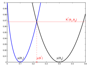
Figure 1: For Bernoulli distributions, the blue and black curves represent respectively $\text{KL}(\mathcal{B}(\mu),\mathcal{B}(\mu_{1}))$ and $\text{KL}(\mathcal{B}(\mu),\mathcal{B}(\mu_{2}))$ as a function of $\mu$. Their intersection gives the value of the Chernoff information between $\mathcal{B}(\mu_{1})$ and $\mathcal{B}(\mu_{2})$, two distributions alternatively parameterized by their natural parameter $\theta_{1}$ and $\theta_{2}$.

3 Improved Lower Bounds for Two-Armed Bandits

Two armed-bandits are of particular interest as they offer a theoretical framework for sequential A/B Testing. A/B Testing is a popular procedure used, for instance, for website optimization: two versions of a web page, say A and B, are empirically compared by being presented to users. Each user is shown only one version $A_{t}\in\{1,2\}$ and provides a real-valued index of the quality of the page, $Z_{t}$, which is modeled as a sample of a probability distribution $\nu_{1}$ or $\nu_{2}$. For example, a standard objective is to determine which web page has the highest conversion rate (probability that a user actually becomes a customer) by receiving binary feedback from the users. In standard A/B Testing algorithms, the two versions are presented equally often. It is thus of particular interest to investigate whether uniform sampling is optimal or not.

Even for two-armed bandits, the upper and lower bounds on the complexity $\kappa_{C}(\nu)$ given in (6) do not match. We propose in this section a refined lower bound on $\kappa_{C}(\nu)$ based on a different change of distribution. This lower bound features a quantity reminiscent of Chernoff information, and we will exhibit algorithms matching (or approximately matching) this new bound in Section 4. Theorem 6 provides a non-asymptotic lower bound on the sample complexity $\mathbb{E}_{\nu}[\tau]$ of any $\delta$-PAC algorithm. It also provides a lower bound on the performance of algorithms using a uniform sampling strategy, which will turn out to be efficient in some cases.

Theorem 6

Let $\mathcal{M}$ be an identifiable class of two-armed bandit models and let $\mathbf{\nu}=(\nu_{1},\nu_{2})\in\mathcal{M}$ be such that $\mu_{1}>\mu_{2}$. Any algorithm that is $\delta$-PAC on $\mathcal{M}$ satisfies, for all $\delta\in)0,1]$,

$$\mathbb{E}_{\nu}[\tau]\geq\frac{1}{c_{*}(\nu)}\log\left(\frac{1}{2.4\delta}\right),\ \ \text{where}\ \ \ c_{*}(\nu):=\inf_{(\nu_{1}^{\prime},\nu_{2}^{\prime})\in\mathcal{M}:\mu_{1}^{\prime}<\mu_{2}^{\prime}}\max\left\{\mathrm{KL}(\nu_{1},\nu_{1}^{\prime}),\mathrm{KL}(\nu_{2},\nu_{2}^{\prime})\right\}.$$

Moreover, any $\delta$-PAC algorithm using a uniform sampling strategy satisfies,

$$\mathbb{E}_{\nu}[\tau]\geq\frac{1}{I_{*}(\nu)}\log\left(\frac{1}{2.4\delta}\right),\ \text{where}\ \ I_{*}(\nu):=\!\inf_{(\nu_{1}^{\prime},\nu_{2}^{\prime})\in\mathcal{M}:\mu^{\prime}_{1}<\mu^{\prime}_{2}}\!\frac{\mathrm{KL}\left(\nu_{1},\nu_{1}^{\prime}\right)+\mathrm{KL}\left(\nu_{2},\nu_{2}^{\prime}\right)}{2}.\hskip 14.22636pt$$ (7)

Obviously, one has $I_{*}(\nu)\leq c_{*}(\nu)$. Theorem 6 implies in particular that $\kappa_{C}(\nu)\geq 1/{c_{*}(\nu)}$. It is possible to give explicit expressions for the quantities $c_{*}(\nu)$ and $I_{*}(\nu)$ for important classes of parametric bandit models that will be considered in the next section.

The class of Gaussian bandits with known variances $\sigma_{1}^{2}$ and $\sigma_{2}^{2}$, further considered in Section 4.1, is

$$\mathcal{M}=\{\nu=\left(\mathcal{N}\left(\mu_{1},\sigma_{1}^{2}\right),\mathcal{N}\left(\mu_{2},\sigma_{2}^{2}\right)\right):(\mu_{1},\mu_{2})\in\mathbb{R}^{2},\mu_{1}\neq\mu_{2}\}.$$ (8)

For this class,

$$\mathrm{KL}(\mathcal{N}\left(\mu_{1},\sigma_{1}\right),\mathcal{N}\left(\mu_{2},\sigma_{2}\right))=\frac{(\mu_{1}-\mu_{2})^{2}}{2\sigma_{2}^{2}}+\frac{1}{2}\left[\frac{\sigma_{1}^{2}}{\sigma_{2}^{2}}-1-\log\frac{\sigma_{1}^{2}}{\sigma_{2}^{2}}\right]$$ (9)

and direct computations yield

$$c_{*}(\nu)=\frac{(\mu_{1}-\mu_{2})^{2}}{2(\sigma_{1}+\sigma_{2})^{2}}\ \ \ \text{and}\ \ \ I_{*}(\nu)=\frac{(\mu_{1}-\mu_{2})^{2}}{4(\sigma_{1}^{2}+\sigma_{2}^{2})}.$$

The observation that, when the variances are different $c_{*}(\nu)>I_{*}(\nu)$, will be shown to imply that strategies based on uniform sampling are sub-optimal (by a factor $1\leq 2(\sigma_{1}^{2}+\sigma_{2}^{2})/(\sigma_{1}+\sigma_{2})^{2}\leq 2$).

The more general class of two-armed exponential bandit models, further considered in Section 4.2, is

$$\mathcal{M}=\{\nu=(\nu_{\theta_{1}},\nu_{\theta_{2}}):(\theta_{1},\theta_{2})\in\Theta^{2},\theta_{1}\neq\theta_{2}\}$$

where $\nu_{\theta_{a}}$ has density $f_{\theta_{a}}$ given by (5). There

$$c_{*}(\nu)=\inf_{\theta\in\Theta}\max\left(\mathrm{K}(\theta_{1},\theta),\mathrm{K}(\theta_{2},\theta)\right)=\mathrm{K}_{*}(\theta_{1},\theta_{2}),$$

where $\mathrm{K}_{*}(\theta_{1},\theta_{2})=\mathrm{K}(\theta_{1},\theta_{*})$, with $\theta_{*}$ is defined by $\mathrm{K}(\theta_{1},\theta_{*})=\mathrm{K}(\theta_{2},\theta_{*})$. This quantity is analogous to the Chernoff information $\mathrm{K}^{*}(\theta_{1},\theta_{2})$ introduced in Section 2 but with ‘reversed’ roles for the arguments. $I_{*}(\nu)$ may also be expressed more explicitly as

$$I_{*}(\nu)=\frac{\mathrm{K}\left(\theta_{1},\overline{\theta}\right)+\mathrm{K}\left(\theta_{2},\overline{\theta}\right)}{2},\ \ \text{where}\ \ \mu(\overline{\theta})=\frac{\mu_{1}+\mu_{2}}{2}.$$

Appendix C provides further useful properties of these quantities and in particular Figure 7 illustrates the property that for two-armed exponential bandit models, the lower bound on $\kappa_{C}(\nu)$ provided by Theorem 6,

$$\kappa_{C}(\nu)\geq\left(\frac{1}{\mathrm{K}_{*}(\theta_{1},\theta_{2})}\right),$$ (10)

is indeed always tighter than the lower bound of Theorem 4,

$$\hskip 56.9055pt\kappa_{C}(\nu)\geq\left(\frac{1}{\mathrm{K}(\theta_{1},\theta_{2})}+\frac{1}{\mathrm{K}(\theta_{2},\theta_{1})}\right).$$ (11)

Interestingly, the changes of distribution used to derive the two results are not the same. On the one hand, for inequality (11), the changes of distribution involved modify a single arm at a time: one of the arms is moved just below (or just above) the other (see Figure 2, left). This is the idea also used, for example, to obtain the lower bound of Lai and Robbins (1985) on the cumulative regret. On the other hand, for inequality (10), both arms are modified at the same time: they are moved close to the common intermediate value $\theta_{*}$ but with a reversed ordering (see Figure 2, right).

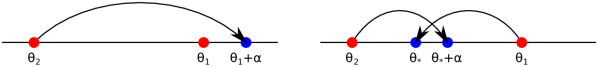
Figure 2: Alternative bandit models considered to obtain the lower bounds of Theorem 4 (left) and Theorem 6 (right).

We now give the proof of Theorem 6, in order to show how easily it follows from Lemma 1.

Proof of Theorem 6. Without loss of generality, one may assume that the bandit model $\nu=(\nu_{1},\nu_{2})$ is such that the best arm is $a^{*}=1$. Consider any alternative bandit model $\nu^{\prime}=(\nu_{1}^{\prime},\nu_{2}^{\prime})$ in which $a^{*}=2$. Let $\mathcal{E}$ be the event $\mathcal{E}=(\hat{\mathcal{S}}_{1}=1)$, which belongs to $\mathcal{F}_{\tau}.$

Let $\mathcal{A}=((A_{t}),\tau,\hat{S}_{1})$ be a $\delta$-PAC algorithm: by assumptions, $\mathbb{P}_{\nu}(\mathcal{E})\geq 1-\delta$ and $\mathbb{P}_{\nu^{\prime}}(\mathcal{E})\leq\delta$. Applying Lemma 1 (with the stopping time $\tau$) and using again the monotonicity properties of $d(x,y)$ and inequality (3)

$$\mathbb{E}_{\nu}[N_{1}]\mathrm{KL}(\nu_{1},\nu_{1}^{\prime})+\mathbb{E}_{\nu}[N_{2}]\mathrm{KL}(\nu_{2},\nu_{2}^{\prime})\geq\log(1/(2.4\delta)).$$ (12)

Using moreover that $\tau=N_{1}+N_{2}$, one has

$$\mathbb{E}_{\nu}[\tau]\geq\frac{\log\left(\frac{1}{2.4\delta}\right)}{\max_{a=1,2}\mathrm{KL}(\nu_{a},\nu_{a}^{\prime})}.$$ (13)

The result follows by optimizing over the possible model $\nu^{\prime}$ satisfying $\mu_{1}^{\prime}<\mu_{2}^{\prime}$ to make the right hand side of the inequality as large as possible. More precisely, for every $\alpha>0$, from the definition of $c_{*}(\nu)$, there exists $\nu^{\prime}_{\alpha}=(\nu_{1}^{\prime},\nu_{2}^{\prime})$ for which

$$\max_{a=1,2}\mathrm{KL}(\nu_{a},\nu_{a}^{\prime})<c_{*}(\nu)+\alpha.$$

Inequality (13) for the particular choice $\nu^{\prime}=\nu^{\prime}_{\alpha}$ yields $\mathbb{E}_{\nu}[\tau]\geq(c_{*}(\nu)+\alpha)^{-1}\log(1/(2.4\delta))$, and the first statement of Theorem 6 follows by letting $\alpha$ go to zero. In the particular case of exponential bandit models, the alternative model consists in choosing $\nu_{1}^{\prime}=\nu_{\theta_{*}}$ and $\nu_{2}^{\prime}=\nu_{\theta_{*}+\epsilon}$ for some $\epsilon$, as illustrated on Figure 2, so that $\max_{a=1,2}\mathrm{KL}(\nu_{a},\nu_{a}^{\prime})$ is of order $\mathrm{K}_{*}(\theta_{1},\theta_{2}).$

When $\mathcal{A}$ uses uniform sampling, using the fact that $\mathbb{E}_{\nu}[N_{1}]=\mathbb{E}[N_{2}]=\mathbb{E}[\tau]/2$ in Equation (12) similarly gives the second statement of Theorem 6.

4 Matching Algorithms for Two-Armed Bandits

For specific instances of two-armed bandit models, we now present algorithms with performance guarantees that closely match the lower bounds of Theorem 6. For Gaussian bandits with known (and possibly different) variances, we describe in Section 4.1 an algorithm termed $\alpha$-Elimination that is optimal and thus makes it possible to determine the complexity $\kappa_{C}(\nu)$. For Bernoulli bandit models, we present in Section 4.2 the SGLRT algorithm that uses uniform sampling and is close to optimal.

4.1 Gaussian Bandit Models

We focus here on the class of two-armed Gaussian bandit models with known variances presented in (8), where $\sigma_{1}$ and $\sigma_{2}$ are fixed. We prove that

$$\kappa_{C}(\nu)=\frac{2(\sigma_{1}+\sigma_{2})^{2}}{(\mu_{1}-\mu_{2})^{2}}$$

by exhibiting a strategy that reaches the performance bound of Theorem 6. This strategy uses non-uniform sampling in case where $\sigma_{1}$ and $\sigma_{2}$ differ. When $\sigma_{1}=\sigma_{2}$, we provide in Theorem 8 an improved stopping rule that is $\delta$-PAC and results in a significant reduction of the expected number of samples used.

The $\alpha$-Elimination algorithm introduced in this Section can also be used in more general two-armed bandit models, where the distribution $\nu_{a}$ is $\sigma_{a}^{2}$-subgaussian. This means that the probability distribution $\nu_{a}$ satisfies

$$\forall\lambda\in\mathbb{R},\ \ \mathbb{E}_{X\sim\nu_{a}}\left[e^{\lambda X}\right]\leq\frac{\lambda^{2}\sigma_{a}^{2}}{2}.$$

This covers in particular the cases of bounded distributions with support in $[0,1]$ (that are $1/4$-subgaussian). In these more general cases, the algorithm enjoys the same theoretical properties: it is $\delta$-PAC and its sample complexity is bounded as in Theorem 9 below.

4.1.1 Equal Variances

We start with the simpler case $\sigma_{1}=\sigma_{2}=\sigma$. Thus, the quantity $I_{*}(\nu)$ introduced in Theorem 6 coincides with $c_{*}(\nu)$, which suggests that uniform sampling could be optimal. A uniform sampling strategy equivalently collects paired samples $(X_{s},Y_{s})$ from both arms. The difference $X_{s}-Y_{s}$ is normally distributed with mean $\mu=\mu_{1}-\mu_{2}$ and a $\delta$-PAC algorithm is equivalent to a sequential test of $H_{0}:(\mu<0)$ versus $H_{1}:(\mu>0)$ such that both type I and type II error probabilities are bounded by $\delta$. Robbins (1970) proposes the stopping rule

$$\tau=\inf\Bigg{\{}t\in 2\mathbb{N}^{*}:\Big{|}\sum_{s=1}^{t/2}(X_{s}-Y_{s})\Big{|}>\sqrt{2\sigma^{2}t\beta(t,\delta)}\Bigg{\}},\text{with}\ \beta(t,\delta)=\frac{t+1}{t}\log\left(\frac{t+1}{2\delta}\right).$$ (14)

The recommendation rule chooses the empirically best arm at time $\tau$. This procedure can be seen as an elimination strategy, in the sense of Jennison et al. (1982). The authors of this paper derive a lower bound on the sample complexity of any $\delta$-PAC elimination strategy (whereas our lower bound applies to any $\delta$-PAC algorithm) which is matched by Robbins’ algorithm: the above stopping rule $\tau$ satisfies

$$\lim_{\delta\rightarrow 0}\frac{\mathbb{E}_{\nu}[\tau]}{\log({1}/{\delta})}=\frac{8\sigma^{2}}{(\mu_{1}-\mu_{2})^{2}}.$$

This value coincide with the lower bound on $\kappa_{C}(\nu)$ of Theorem 6 in the case of two-armed Gaussian distributions with similar known variance $\sigma^{2}$. This proves that in this case, Robbins’ rule (14) is not only optimal among the class of elimination strategies, but also among the class of $\delta$-PAC algorithm.

Any $\delta$-PAC elimination strategy that uses a threshold function (or exploration rate) $\beta(t,\delta)$ smaller than Robbins’ also matches our asymptotic lower bound, while stopping earlier than the latter. From a practical point of view, it is therefore interesting to exhibit smaller exploration rates that preserve the $\delta$-PAC property. The failure probability of such an algorithm is upper bounded, for example when $\mu_{1}<\mu_{2}$, by

$$\mathbb{P}_{\nu}\left(\exists k\in\mathbb{N}:\sum_{s=1}^{k}\frac{X_{s}-Y_{s}-(\mu_{1}-\mu_{2})}{\sqrt{2\sigma^{2}}}>\sqrt{2k\beta(2k,\delta)}\right)=\mathbb{P}\left(\exists k\in\mathbb{N}:S_{k}>\sqrt{2k\beta(2k,\delta)}\right)$$ (15)

where $S_{k}$ is a sum of $k$ i.i.d. variables of distribution $\mathcal{N}\left(0,1\right)$. Robbins (1970) obtains a non-explicit confidence region of risk at most $\delta$ by choosing $\beta(2k,\delta)=\log\left({\log(k)}/{\delta}\right)+o(\log\log(k))$. The dependency in $k$ is in some sense optimal, because the Law of Iterated Logarithm (LIL) states that $\limsup_{k\rightarrow\infty}{S_{k}}/\sqrt{2k\log\log(k)}=1$ almost surely. In this paper, we propose a new deviation inequality for a martingale with sub-Gaussian increments, stated as Lemma 7, that permits to build an explicit confidence region reminiscent of the LIL. A related result was recently derived independently by Jamieson et al. (2014).

Lemma 7

Let $\zeta(u)=\sum_{k\geq 1}k^{-u}$. Let $X_{1},X_{2},\dots$ be independent random variables such that, for all $\lambda\in\mathbb{R}$, $\phi(\lambda):=\log\mathbb{E}[\exp(\lambda X_{1})]\leq\lambda^{2}\sigma^{2}/2$. For every positive integer $t$ let $S_{t}=X_{1}+\dots+X_{t}$. Then, for all $\eta>1$ and $x\geq\frac{8}{(e-1)^{2}}$,

$$\mathbb{P}\left(\exists t\in\mathbb{N}^{*}:{S_{t}}>\sqrt{2\sigma^{2}t(x+\eta\log\log(et))}\right)\leq\sqrt{e}\,\zeta\left(\eta\left(1-\frac{1}{2x}\right)\right)\left(\frac{\sqrt{x}}{2\sqrt{2}}+1\right)^{\eta}\exp(-x).$$

Lemma 7 allows to prove Theorem 8 below, as detailed in Appendix E, where we also provide a proof of Lemma 7.

Theorem 8

For $\delta\leq 0.1$, with

$$\beta(t,\delta)=\log({1}/{\delta})+3\log\log({1}/{\delta})+(3/2)\log(\log(et/2)),$$ (16)

the elimination strategy is $\delta$-PAC.

We refer to Section 6 for numerical simulations that illustrate the significant savings (in the average number of samples needed to reach a decision) resulting from the use of the less conservative exploration rate allowed by Theorem 8.

4.1.2 Mismatched Variances

In the case where $\sigma_{1}\neq\sigma_{2}$, we rely on the $\alpha$-Elimination strategy, described in Algorithm 1 below. For $a=1,2$, $\hat{\mu}_{a}(t)$ denotes the empirical mean of the samples gathered from arm $a$ up to time $t$. The algorithm is based on a non-uniform sampling strategy governed by the parameter $\alpha\in(0,1)$, that maintains the proportion of draws of arm 1 close to $\alpha$. At the end of every round $t$, $N_{1}(t)=\lceil\alpha t\rceil$, $N_{2}(t)=t-\lceil\alpha t\rceil$ and $\hat{\mu}_{1}(t)-\hat{\mu}_{2}(t)\sim\mathcal{N}\left(\mu_{1}-\mu_{2},\sigma_{t}^{2}(\alpha)\right)$ (where $\sigma_{t}^{2}(\alpha)$ is defined at line 6 of Algorithm 1). The sampling schedule used here is thus deterministic.

Algorithm 1 $\alpha$-Elimination

0:  Exploration function $\beta(t,\delta)$, parameter $\alpha$.

1:  Initialization: $\hat{\mu}_{1}(0)=\hat{\mu}_{2}(0)=0$, $\sigma^{2}_{0}(\alpha)=1$, $t=0$

2:  while $|\hat{\mu}_{1}(t)-\hat{\mu}_{2}(t)|\leq\sqrt{2\sigma^{2}_{t}(\alpha)\beta(t,\delta)}$ do

3:     $t\leftarrow t+1$.

4:     If $\lceil\alpha t\rceil=\lceil\alpha(t-1)\rceil$, $A_{t}\leftarrow 2$, else $A_{t}\leftarrow 1$

5:     Observe $Z_{t}\sim\nu_{A_{t}}$ and compute the empirical means $\hat{\mu}_{1}(t)$ and $\hat{\mu}_{2}(t)$

6:     Compute $\sigma_{t}^{2}(\alpha)=\sigma_{1}^{2}/\lceil\alpha t\rceil+\sigma_{2}^{2}/(t-\lceil\alpha t\rceil)$

7:  end while

8:  return  $\underset{a=1,2}{\text{argmax}}\ \hat{\mu}_{a}(t)$

Theorem 9 shows that an optimal allocation of samples between the two arms consists in maintaining the proportion of draws of arm 1 close to $\sigma_{1}/(\sigma_{1}+\sigma_{2})$ (which is also the case in the fixed-budget setting, see Section 5.1). Indeed, for $\alpha=\sigma_{1}/(\sigma_{1}+\sigma_{2})$, the $\alpha$-elimination algorithm is $\delta$-PAC with a suitable exploration rate and (almost) matches the lower bound on $\mathbb{E}_{\nu}[\tau]$, at least asymptotically when $\delta\rightarrow 0$. Its proof can be found in Appendix D.

Theorem 9

If $\alpha=\sigma_{1}/(\sigma_{1}+\sigma_{2})$, the $\alpha$-elimination strategy using the exploration rate $\beta(t,\delta)=\log\frac{t}{\delta}+2\log\log(6t)$ is $\delta$-PAC on $\mathcal{M}$ and satisfies, for every $\nu\in\mathcal{M}$, for every $\epsilon>0$,

$$\mathbb{E}_{\nu}[\tau]\leq(1+\epsilon)\frac{2(\sigma_{1}+\sigma_{2})^{2}}{(\mu_{1}-\mu_{2})^{2}}\log\left(\frac{1}{\delta}\right)+\underset{\delta\rightarrow 0}{o_{\epsilon}}\left(\log\left(\frac{1}{\delta}\right)\right).$$

Remark 10

When $\sigma_{1}=\sigma_{2}$, $1/2$-elimination reduces, up to rounding effects, to the elimination procedure described in Section 4.1.1, for which Theorem 8 suggests an exploration rate of order $\log(\log(t)/\delta)$. As the feasibility of this exploration rate when $\sigma_{1}\neq\sigma_{2}$ is yet to be established, we focus on Gaussian bandits with equal variances in the numerical experiments of Section 6.

4.2 Bernoulli Bandit Models

We consider in this section the class of Bernoulli bandit models

$$\mathcal{M}=\{\nu=\left(\mathcal{B}(\mu_{1}),\mathcal{B}(\mu_{2})\right):(\mu_{1},\mu_{2})\in(0;1)^{2},\mu_{1}\neq\mu_{2}\},$$

where each arm can be alternatively parameterized by the natural parameter of the exponential family, $\theta_{a}=\log({\mu_{a}}/{(1-\mu_{a})})$. Observing that in this particular case little can be gained by departing from uniform sampling, we consider the SGLRT algorithm (to be defined below) that uses uniform sampling together with a stopping rule that is not based on the mere difference of the empirical means.

For Bernoulli bandit models, the quantities $I_{*}(\nu)$ and $c_{*}(\nu)$ introduced in Theorem 6 happen to be practically very close (see Figure 3 in Section 5 below). There is thus a strong incentive to use uniform sampling and in the rest of this section we consider algorithms that aim at matching the bound (7) of Theorem 6—that is, $\mathbb{E}_{\nu}[\tau]\leq\log(1/\delta)/I_{*}(\nu)$, at least for small values of $\delta$—, which provides an upper bound on $\kappa_{C}(\nu)$ that is very close to $1/c_{*}(\nu)$. For simplicity, as $I_{*}(\nu)$ is here a function of the means of the arms only, we will denote $I_{*}(\nu)$ by $I_{*}(\mu_{1},\mu_{2})$.

When the arms are sampled uniformly, finding an algorithm that matches the bound of (7) boils down to determining a proper stopping rule. In all the algorithms studied so far, the stopping rule was based on the difference of the empirical means of the arms. For Bernoulli arms the 1/2-Elimination procedure described in Algorithm 1 can be used, as each distribution $\nu_{a}$ is bounded and therefore 1/4-subgaussian. More precisely, with $\beta(t,\delta)$ as in Theorem 8, the algorithm stopping at the first time $t$ such that

$$\hat{\mu}_{1}(t)-\hat{\mu}_{2}(t)>\sqrt{{2\beta(t,\delta)}/{t}}$$

has its sample complexity bounded by ${2}/{(\mu_{1}-\mu_{2})^{2}}\log({1}/{\delta})+o\left(\log({1}/{\delta})\right)$. Yet, Pinsker’s inequality implies that $I_{*}(\mu_{1},\mu_{2})>(\mu_{1}-\mu_{2})^{2}/2$ and this algorithm is thus not optimal with respect to the bound (7) of Theorem 6. The approximation $I_{*}(\mu_{1},\mu_{2})=(\mu_{1}-\mu_{2})^{2}/(8\mu_{1}(1-\mu_{1}))+o\left((\mu_{1}-\mu_{2})^{2}\right)$ suggests that the loss with respect to the optimal error exponent is particularly significant when both means are close to 0 or 1.

Algorithm 2 Sequential Generalized Likelihood Ratio Test (SGLRT)

0:  Exploration function $\beta(t,\delta)$.

1:  Initialization: $\hat{\mu}_{1}(0)=\hat{\mu}_{2}(0)=0$. $t=0$.

2:  while ($tI_{*}(\hat{\mu}_{1}(t),\hat{\mu}_{2}(t))\leq\beta(t,\delta))\bigcup(t=1\ (mod.\ 2))$ do

3:     $t=t+1$. $A_{t}=t\ (mod.\ 2)$.

4:     Observe $Z_{t}\sim\nu_{A_{t}}$ and compute the empirical means $\hat{\mu}_{1}(t)$ and $\hat{\mu}_{2}(t)$.

5:  end while

6:  return  $a=\underset{a=1,2}{\text{argmax}}\ \hat{\mu}_{a}(t)$.

To circumvent this drawback, we propose the SGLRT (for Sequential Generalized Likelihood Ratio Test) stopping rule, described in Algorithm 2. The appearance of $I_{*}$ in the stopping criterion of Algorithm 2 is a consequence of the observation that it is related to the generalized likelihood ratio statistic for testing the equality of two Bernoulli proportions. To test $H_{0}:(\mu_{1}=\mu_{2})$ against $H_{1}:(\mu_{1}\neq\mu_{2})$ based on $t/2$ paired samples of the arms $W_{s}=(X_{s},Y_{s})$, the Generalized Likelihood Ratio Test (GLRT) rejects $H_{0}$ when

$$\frac{\max_{\mu_{1},\mu_{2}:\mu_{1}=\mu_{2}}L(W_{1},\dots,W_{t/2};\mu_{1},\mu_{2})}{\max_{\mu_{1},\mu_{2}}L(W_{1},\dots,W_{t/2};\mu_{1},\mu_{2})}<z_{\delta},$$

where $L(W_{1},\dots,W_{t/2};\mu_{1},\mu_{2})$ denotes the likelihood of the observations given parameters $\mu_{1}$ and $\mu_{2}$. It can be checked that the ratio that appears in the last display is equal to $\exp(-tI_{*}(\hat{\mu}_{1,t/2},\hat{\mu}_{2,t/2}))$. This equality is a consequence of the rewriting

$$I_{*}(x,y) = H\left(\frac{x+y}{2}\right)-\frac{1}{2}\left[H\left({x}\right)+H\left({y}\right)\right],$$

where $H(x)=-x\log(x)-(1-x)\log(1-x)$ denotes the binary entropy function. Hence, Algorithm (2) can be interpreted as a sequential version of the GLRT with (varying) threshold $z_{t,\delta}=\exp(-\beta(t,\delta))$.

Elements of analysis of the SGLRT. The SGLRT algorithm is also related to the KL-LUCB algorithm of Kaufmann and Kalyanakrishnan (2013). A closer examination of the KL-LUCB stopping criterion reveals that, in the specific case of two-armed bandits, it is equivalent to stopping when $t\mathrm{KL}_{*}(\mathcal{B}(\hat{\mu}_{1}(t)),\mathcal{B}(\hat{\mu}_{2}(t)))$ gets larger than some threshold. We also mentioned the fact that $\mathrm{KL}_{*}(\mathcal{B}(x),\mathcal{B}(y))$ and $I_{*}(x,y)$ are very close (see Figure 3). Using results from Kaufmann and Kalyanakrishnan (2013), one can thus prove (see Appendix F) the following lemma.

Lemma 11

With the exploration rate

$$\beta(t,\delta)=2\log\left(\frac{t(\log(3t))^{2}}{\delta}\right)$$

the SGLRT algorithm is $\delta$-PAC.

For this exploration rate, we were able to obtain the following asymptotic guarantee on the stopping time $\tau$ of Algorithm 2:

$$\forall\epsilon>0,\ \ \limsup_{\delta\rightarrow 0}\frac{\tau}{\log(1/\delta)}\leq\frac{2(1+\epsilon)}{I_{*}(\mu_{1},\mu_{2})}\ \ a.s.$$

(see Lemma 26 in Appendix F for the proof of this result). By analogy with the result of Theorem 8 we conjecture that the analysis of Kaufmann and Kalyanakrishnan (2013)—on which the result of Lemma 11 is based—is too conservative and that the use of an exploration rate of order $\log(\log(t)/\delta)$ should also lead to a $\delta$-PAC algorithm. This conjecture is supported by the numerical experiments reported in Section 6 below. Besides, for this choice of exploration rate, Lemma 26 also shows that

$$\forall\epsilon>0,\ \ \limsup_{\delta\rightarrow 0}\frac{\tau}{\log(1/\delta)}\leq\frac{(1+\epsilon)}{I_{*}(\mu_{1},\mu_{2})}\ \ a.s..$$

5 The Fixed-Budget Setting

In this section, we focus on the fixed-budget setting and we provide new upper and lower bounds on the complexity term $\kappa_{B}(\nu)$.

For two-armed bandits, we obtain in Theorem 12 lower bounds analogous to those of Theorem 6 in the fixed-confidence setting. We present matching algorithms for Gaussian and Bernoulli bandits. This allows for a comparison between the fixed-budget and fixed-confidence setting in these specific cases. More specifically, we show that $\kappa_{B}(\nu)=\kappa_{C}(\nu)$ for Gaussian bandit models, whereas $\kappa_{C}(\nu)>\kappa_{B}(\nu)$ for Bernoulli bandit models.

When $K>2$ and $m\geq 1$, we present a first step towards obtaining more general results, by providing lower bounds on the probability of error $p_{t}(\nu)$ for Gaussian bandits with equal variances.

5.1 Comparison of the Complexities for Two-Armed Bandits

We present here an asymptotic lower bound on $p_{t}(\nu)$ that directly yields a lower bound on $\kappa_{B}(\nu)$. Moreover, we provide a lower bound on the failure probability of consistent algorithms using uniform sampling. The proof of Theorem 12 bears similarities with that of Theorem 6, and we provide it in Appendix G.1. However, it is important to note that the informational quantities $c^{*}(\nu)$ and $I^{*}(\nu)$ defined in Theorem 12 are in general different from the quantities $c_{*}(\nu)$ and $I_{*}(\nu)$ previously defined for the fixed-confidence setting (see Theorem 6). Appendix C contains a few additional elements of comparison between these quantities in the case of one-parameter exponential families of distributions.

Theorem 12

Let $\mathbf{\nu}=(\nu_{1},\nu_{2})$ be a two-armed bandit model such that $\mu_{1}>\mu_{2}$. In the fixed-budget setting, any consistent algorithm satisfies

$$\limsup_{t\rightarrow\infty}-\frac{1}{t}\log p_{t}(\nu)\leq c^{*}(\nu),\ \ \ \text{where}\ \ \ c^{*}(\nu):=\inf_{(\nu_{1}^{\prime},\nu_{2}^{\prime})\in\mathcal{M}:\mu^{\prime}_{1}<\mu^{\prime}_{2}}\max\left\{\mathrm{KL}(\nu_{1}^{\prime},\nu_{1}),\mathrm{KL}(\nu_{2}^{\prime},\nu_{2})\right\}.$$

Moreover, any consistent algorithm using a uniform sampling strategy satisfies

$$\limsup_{t\rightarrow\infty}-\frac{1}{t}\log p_{t}(\nu)\leq I^{*}(\nu),\ \ \ \text{where}\ \ \ I^{*}(\nu):=\inf_{(\nu_{1}^{\prime},\nu_{2}^{\prime})\in\mathcal{M}:\mu^{\prime}_{1}<\mu^{\prime}_{2}}\frac{\mathrm{KL}\left(\nu_{1}^{\prime},\nu_{1}\right)+\mathrm{KL}\left(\nu_{2}^{\prime},\nu_{2}\right)}{2}.\hskip 14.22636pt$$ (17)

Gaussian distributions. As   the   Kullback-Leibler   divergence   between two   Gaussian distributions—(9)—is symmetric with respect to the means when the variances are held fixed, it holds that $c^{*}(\nu)=c_{*}(\nu)$. To find a matching algorithm, we introduce the simple family of static strategies that draw $n_{1}$ samples from arm 1 followed by $n_{2}=t-n_{1}$ samples of arm 2, and then choose arm 1 if $\hat{\mu}_{1,n_{1}}>\hat{\mu}_{2,n_{2}}$, where $\hat{\mu}_{i,n_{i}}$ denotes the empirical mean of the $n_{i}$ samples from arm $i$. Assume for instance that $\mu_{1}>\mu_{2}$. Since $\hat{\mu}_{1,n_{1}}-\hat{\mu}_{2,n_{2}}-\mu_{1}+\mu_{2}\sim\mathcal{N}\left(0,{\sigma_{1}^{2}}/{n_{1}}+{\sigma_{2}^{2}}/{n_{2}}\right)$, the probability of error of such a strategy is upper bounded by

$$\mathbb{P}\left(\hat{\mu}_{1,n_{1}}<\hat{\mu}_{2,n_{2}}\right) \leq \exp\left(-\left(\frac{\sigma_{1}^{2}}{n_{1}}+\frac{\sigma_{2}^{2}}{n_{2}}\right)^{-1}\frac{(\mu_{1}-\mu_{2})^{2}}{2}\right).$$

The right hand side is minimized when $n_{1}/(n_{1}+n_{2})={\sigma_{1}}/{(\sigma_{1}+\sigma_{2})}$, and the static strategy drawing $n_{1}=\left\lceil\sigma_{1}t/(\sigma_{1}+\sigma_{2})\right\rceil$ times arm 1 is such that

$$\liminf_{t\rightarrow\infty}-\frac{1}{t}\log p_{t}(\nu)\geq\frac{(\mu_{1}-\mu_{2})^{2}}{2(\sigma_{1}+\sigma_{2})^{2}}=c^{*}(\nu)\;.$$

This shows in particular that for Gaussian distributions the two complexities are equal:

$$\kappa_{B}(\nu)=\kappa_{C}(\nu)=\frac{2(\sigma_{1}+\sigma_{2})^{2}}{(\mu_{1}-\mu_{2})^{2}}.$$

Exponential families. For exponential family bandit models, it can be observed that

$$c^{*}(\nu)=\inf_{\theta\in\Theta}\max\left(\mathrm{K}(\theta,\theta_{1}),\mathrm{K}(\theta,\theta_{2})\right)=\mathrm{K}^{*}(\theta_{1},\theta_{2}),$$

where $\mathrm{K}^{*}(\theta_{1},\theta_{2})$ is the Chernoff information between the distributions $\nu_{\theta_{1}}$ and $\nu_{\theta_{2}}$. We recall that $\mathrm{K}^{*}(\theta_{1},\theta_{2})=\mathrm{K}(\theta^{*},\theta_{1})$, where $\theta^{*}$ is defined by $\mathrm{K}(\theta^{*},\theta_{1})=\mathrm{K}(\theta^{*},\theta_{2})$. Moreover, one has

$$I^{*}(\nu)=\frac{\mathrm{K}\left(\frac{\theta_{1}+\theta_{2}}{2},\theta_{1}\right)+\mathrm{K}\left(\frac{\theta_{1}+\theta_{2}}{2},\theta_{2}\right)}{2}.$$

In particular, the quantity $c^{*}(\nu)=\mathrm{K}^{*}(\theta_{1},\theta_{2})$ does not always coincide with the quantity $c_{*}(\nu)=\mathrm{K}_{*}(\theta_{1},\theta_{2})$ defined in Theorem 6. More precisely, $c_{*}(\nu)$ and $c^{*}(\nu)$ are equal when the log-partition function $b(\theta)$ is (Fenchel) self-conjugate, which is the case for Gaussian and exponential variables (see Appendix C). However, for Bernoulli distributions, it can be checked that $c^{*}(\nu)>c_{*}(\nu)$. By exhibiting a matching strategy in the fixed-budget setting (Theorem 13), we show that this implies that $\kappa_{C}(\nu)>\kappa_{B}(\nu)$ in the Bernoulli case (Theorem 14). We also show that in this case, only little can be gained by departing from uniform sampling.

Theorem 13

Consider a two-armed exponential bandit model and $\alpha(\theta_{1},\theta_{2})$ be defined by

$$\alpha(\theta_{1},\theta_{2})=\frac{\theta^{*}-\theta_{1}}{\theta_{2}-\theta_{1}}\ \ \ \text{where}\ \ \mathrm{K}(\theta^{*},\theta_{1})=\mathrm{K}(\theta^{*},\theta_{2}).$$

For all $t$, the static strategy that allocates $\left\lceil\alpha(\theta_{1},\theta_{2})t\right\rceil$ samples to arm 1, and recommends the empirical best arm, satisfies $p_{t}(\nu)\leq\exp(-tK^{*}(\theta_{1},\theta_{2}))$.

Theorem 13, whose proof can be found in Appendix G.2, shows in particular that for every exponential family bandit model there exists a consistent static strategy such that

$$\liminf_{t\rightarrow\infty}-\frac{1}{t}\log p_{t}\geq\mathrm{K}^{*}(\theta_{1},\theta_{2}),\ \ \ \text{and hence that}\ \ \kappa_{B}(\nu)=\frac{1}{\mathrm{K}^{*}(\theta_{1},\theta_{2})}.$$

By combining this observation with Theorem 6 and the fact that, $\mathrm{K}_{*}(\theta_{1},\theta_{2})<\mathrm{K}^{*}(\theta_{1},\theta_{2})$ for Bernoulli distributions, one obtains the following inequality.

Theorem 14

For two-armed Bernoulli bandit models, $\kappa_{C}(\nu)>\kappa_{B}(\nu)$.

Note that we have determined the complexity of the fixed-budget setting by exhibiting an algorithm (leading to an upper bound on $\kappa_{B}$) that is of limited practical interest for Bernoulli bandit models. Indeed, the optimal static strategy defined in Theorem 13 requires the knowledge of the quantity $\alpha(\theta_{1},\theta_{2})$, that depends on the unknown means of the arms. So far, it is not known whether there exists a universal strategy, that would satisfy $p_{t}(\nu)\leq\exp(-\mathrm{K}^{*}(\theta_{1},\theta_{2})t)$ on every Bernoulli bandit model.

However, Lemma 27 shows that the strategy that uses uniform sampling and recommends the empirical best-arm satisfies $p_{t}(\nu)\leq\exp(-I^{*}(\nu)t)$, and matches the bound (17) of Theorem 12 (see Remark 28 in Appendix G.2). The fact that, just as in the fixed-confidence setting $I^{*}(\nu)$ is very close to $c^{*}(\nu)$ shows that the problem-dependent optimal strategy described above can be approximated by a very simple, universal algorithm that samples the arms uniformly. Figure 3 represents the different informational functions $c_{*},I_{*},c^{*}$ and $I^{*}$ when the mean $\mu_{1}$ varies, for two fixed values of $\mu_{2}$. It can be observed that $c^{*}(\nu)$ and $c_{*}(\nu)$ are almost indistinguishable from $I^{*}(\nu)$ and $I_{*}(\nu)$, respectively, while there is a gap between $c^{*}(\nu)$ and $c_{*}(\nu)$.

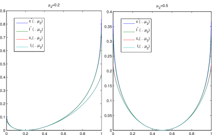
Figure 3: Comparison of different informational quantities for Bernoulli bandit models.

5.2 Lower Bound on $p_{t}(\nu)$ in More General Cases

Theorem 12 provides a direct counterpart to Theorem 6, allowing for a complete comparison between the fixed confidence and fixed budget settings in the case of two-armed bandits. However, we were not able to obtain a general lower bound for $K$-armed bandit that would be directly comparable to that of Theorem 4 in the fixed budget setting. Using Lemma 15 stated below (a variant of Lemma 1 proved in Appendix A.2), we were nonetheless able to derive tighter, non-asymptotic, lower bounds on $p_{t}(\nu)$ in the particular case of Gaussian bandit models with equal known variance, $\mathcal{M}_{m}=\{\nu=(\nu_{1},\dots,\nu_{K}):\nu_{a}=\mathcal{N}\left(\mu_{a},\sigma^{2}\right),\mu_{a}\in\mathbb{R},\mu_{[m]}\neq\mu_{[m+1]}\}$.

Lemma 15

Let $\nu$ and $\nu^{\prime}$ be two bandit models such that $\mathcal{S}_{m}^{*}(\nu)\neq\mathcal{S}_{m}^{*}(\nu^{\prime})$. Then

$$\max\left(\mathbb{P}_{\nu}(\mathcal{S}\neq\mathcal{S}_{m}^{*}(\nu)),\mathbb{P}_{\nu^{\prime}}(\mathcal{S}\neq\mathcal{S}_{m}^{*}(\nu^{\prime}))\right)\geq\frac{1}{4}\exp\left(-\sum_{a=1}^{K}\mathbb{E}_{\nu}[N_{a}]\mathrm{KL}(\nu_{a},\nu^{\prime}_{a})\right).$$

Theorem 16

Let $\nu$ be a Gaussian bandit model such that $\mu_{1}>\mu_{2}\geq\dots\geq\mu_{K}$ and let

$$H^{\prime}(\nu)=\sum_{a=2}^{K}\frac{2\sigma^{2}}{(\mu_{1}-\mu_{a})^{2}}.$$

There exists a bandit model $\nu^{[a]}$, $a\in\{2,\dots,K\}$, (see Figure 4) which satisfies $H^{\prime}(\nu^{[a]})\leq H^{\prime}(\nu)$ and is such that

$$\max\left(p_{t}(\nu),p_{t}(\nu^{[a]})\right)\geq\exp\left(-\frac{4t}{H^{\prime}(\nu)}\right).$$

This result is to be compared to the lower bound of Audibert et al. (2010). While Theorem 16 does not really provide a lower bound on $\kappa_{B}(\nu)$, the complexity term $H(\nu)$ is close to the quantity that appears in Theorem 4 for the fixed-confidence setting (in the Gaussian case), which improves over the term $H_{2}(\nu)=\max_{i:\mu_{[i]}<\mu_{[1]}}{i}{(\mu_{[1]}-\mu_{[i]})^{-2}}$ featured in Theorem 4 of Audibert et al. (2010).

For $m>1$, building on the same ideas, Theorem 17 provides a first lower bound, which we believe leaves room for improvement.

Theorem 17

Let $\nu$ be such that $\mu_{1}>\dots\mu_{m}>\mu_{m+1}>\dots>\mu_{K}$ and let

$$H^{+}(\nu)=\sum_{a=1}^{m}\frac{2\sigma^{2}}{(\mu_{a}-\mu_{m+1})^{2}},\ \ \ H^{-}(\nu)=\sum_{a=m+1}^{K}\frac{2\sigma^{2}}{(\mu_{m}-\mu_{a})^{2}},\ \ \ \text{and}\ \ \ H(\nu)=H^{+}(\nu)+H^{-}(\nu).$$

There exists $a\in\{1,\dots,m\}$ and $b\in\{m+1,\dots K\}$ such that the bandit model $\nu^{[a,b]}$ described on Figure 4 satisfies $H(\nu^{[a,b]})<H(\nu)$ and is such that

$$\max\left(p_{t}(\nu),p_{t}(\nu^{[a,b]})\right)\geq\frac{1}{4}\exp\left(-\frac{4t}{\tilde{H}(\nu)}\right),\ \ \text{where}\ \ \tilde{H}(\nu)=\frac{H(\nu)\min(H^{+}(\nu),H^{-}(\nu))}{H(\nu)+\min(H^{+}(\nu),H^{-}(\nu))}.$$

         

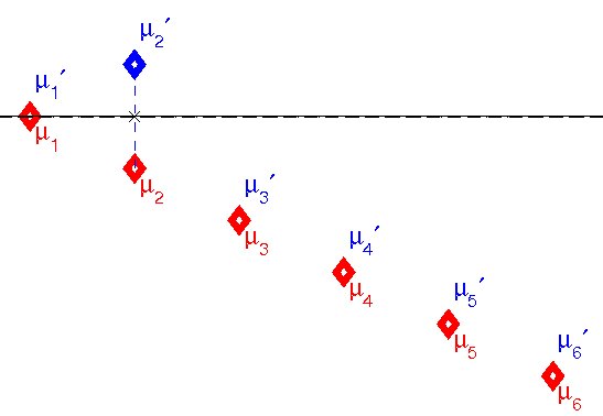
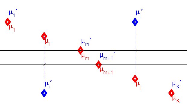
Figure 4: Left: bandit models $\nu$, in red, and $\nu^{[2]}$, in blue (Theorem 16). Right: bandit models $\nu$, in red, and $\nu^{[i,j]}$, in blue (Theorem 17).

The proofs of Theorem 16 and Theorem 17 are very similar. For this reason, we provide in Appendix G.3 only the latter. Introducing the gaps $\Delta_{a}$ defined in (2), the precise definition of the modified problems $\nu^{[a]}$ and $\nu^{[a,b]}$ in the statement of the two results is:

$$\nu^{[a]}:\ \left\{\begin{array}[]{ccl}\mu_{k}^{\prime}&=&\mu_{k}\ \text{for all}\ k\neq a\\ \mu_{a}^{\prime}&=&\mu_{a}+2\Delta_{a}\end{array}\right.\ \ \text{and}\ \ \ \ \nu^{[a,b]}:\ \left\{\begin{array}[]{ccl}\mu_{k}^{\prime}&=&\mu_{k}\ \text{for all}\ k\notin\{a,b\}\\ \mu_{a}^{\prime}&=&\mu_{a}-2\Delta_{b}\\ \mu^{\prime}_{b}&=&\mu_{b}+2\Delta_{a}\end{array}\right..$$

6 Numerical Experiments

In this section, we focus on two-armed models and provide experimental experiments designed to compare the fixed-budget and fixed-confidence settings (in the Gaussian and Bernoulli cases) and to illustrate the improvement resulting from the adoption of the reduced exploration rate of Theorem 8.

In Figure 5, we consider two Gaussian bandit models with known common variance: the ‘easy’ one is $\{\mathcal{N}\left(0.5,0.25\right),\mathcal{N}\left(0,0.25\right)\}$, corresponding to $\kappa_{C}=\kappa_{B}=\kappa=8$, on the left; and the ‘difficult’ one is $\{\mathcal{N}\left(0.01,0.25\right),\mathcal{N}\left(0,0.25\right)\}$, that is $\kappa=2\times 10^{4}$, on the right. In the fixed-budget setting, stars (’*’) report the probability of error $p_{n}(\nu)$ as a function of $n$. In the fixed-confidence setting, we plot both the empirical probability of error by circles (’O’) and the specified maximal error probability $\delta$ by crosses (’X’) as a function of the empirical average of the running times. Note the logarithmic scale used for the probabilities on the y-axis. All results are averaged over $N=10^{6}$ independent Monte Carlo replications. For comparison purposes, a plain line represents the theoretical rate $t\mapsto\exp(-t(1/\kappa))$ which is a straight line on the log scale.

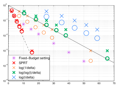
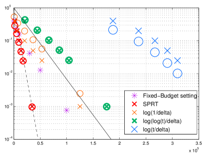
Figure 5: Experimental results for Gaussian bandit models

In the fixed-confidence setting, we report results for elimination algorithms of the form (14) for three different exploration rates $\beta(t,\delta)$. The exploration rate we consider are: the provably-PAC rate of Robbins’ algorithm $\log({t}/{\delta})$ (large blue symbols), the conjectured optimal exploration rate $\log({(\log(t)+1)}/{\delta})$, almost provably $\delta$-PAC according to Theorem 8 (bold green symbols), and the rate $\log({1}/{\delta})$, which would be appropriate if we were to perform the stopping test only at a single pre-specified time (orange symbols). For each algorithm, the log probability of error is approximately a linear function of the number of samples, with a slope close to $-1/\kappa$, where $\kappa$ is the complexity. A first observation is that the ’traditional’ rate of $\log({t}/{\delta})$ is much too conservative, with running times for the difficult problem (right plot) which are about three times longer than those of other methods for comparable error rates. As expected, the rate $\log((\log(t)+1)/\delta)$ significantly reduces the running times while maintaining proper control of the probability of failure, with empirical error rates (’O’ symbols) below the corresponding confidence parameters $\delta$ (represented by ’X’ symbols). Conversely, the use of the non-sequential testing threshold $\log(1/\delta)$ seems too risky, as one can observe that the empirical probability of error may be larger than $\delta$ on difficult problems. To illustrate the gain in sample complexity resulting from the knowledge of the means, we also represented in red the performance of the SPRT algorithm mentioned in the introduction of Section 5 along with the theoretical relation between the probability of error and the expected number of samples, materialized as a dashed line. The SPRT stops for $t$ such that $|(\mu_{1}-\mu_{2})(S_{1,t/2}-S_{2,t/2})|>\log(1/\delta)$.

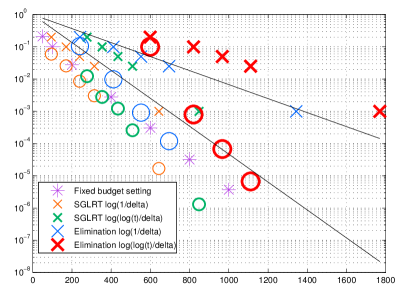
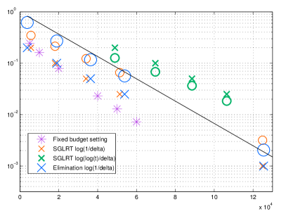
Figure 6: Results for Bernoulli bandit models: $0.2-0.1$ (left) and $0.51-0.5$ (right).

Robbins’ algorithm is $\delta$-PAC and matches the complexity (which is illustrated by the slope of the measures), though in practice the use of the exploration rate $\log((\log(t)+1)/\delta)$ leads to huge gain in terms of number of samples used. It is important to keep in mind that running times play the same role as error exponents and hence the threefold increase of average running times observed on the rightmost plot of Figure 5 when using $\beta(t,\delta)=\log({t}/{\delta})$ is really prohibitive.

On Figure 6, we compare on two Bernoulli bandit models the performance of the SGLRT algorithm described in Section 4.2 (Algorithm 2) using two different exploration rates, $\log(1/\delta)$ and $\log((\log(t)+1)/\delta)$, to the 1/2-elimination stopping rule (Algorithm 1) that stops when the difference of empirical means exceeds the threshold $\sqrt{2\beta(t,\delta)/t}$ (for the same exploration rates). Plain lines also materialize the theoretical optimal rate $t\mapsto\exp(-t/\kappa_{C}(\nu))$ and the rate attained by the 1/2-Elimination algorithm $t\mapsto\exp(-t/\kappa^{\prime})$, where $\kappa^{\prime}=2/(\mu_{1}-\mu_{2})^{2}$. On the bandit model $0.51-0.5$ (right) these two rates are very close and SGLRT mostly coincides with Elimination, but on the bandit model $0.2-0.1$ (left) the practical gain of the use of a more sophisticated stopping strategy is well illustrated. Besides, our experiments show that SGLRT using $\log((\log(t)+1)/\delta)$ is $\delta$-PAC on both the (relatively) easy and difficult problems we consider, unlike the other algorithms considered.

If one compares the results for the fixed-budget setting (in purple) to those for the best $\delta$-PAC algorithm (or conjectured $\delta$-PAC for SGLRT in the Bernoulli case), in green, one can observe that to obtain the same probability of error, the fixed-confidence algorithm usually needs an average number of samples that is about twice larger than the deterministic number of samples required by the fixed-budget setting algorithm. This remark should be related to the fact that a $\delta$-PAC algorithm is designed to be uniformly good across all problems, whereas consistency is a weak requirement in the fixed-budget setting: any strategy that draws both arm infinitely often and recommends the empirical best is consistent. Figure 5 also shows that when the values of $\mu_{1}$ and $\mu_{2}$ are unknown, the sequential version of the test is no more preferable to its batch counterpart and can even become much worse if the exploration rate $\beta(t,\delta)$ is chosen too conservatively. This observation should be mitigated by the fact that the sequential (or fixed-confidence) approach is adaptive with respect to the difficulty of the problem whereas it is impossible to predict the efficiency of a batch (or fixed-budget) experiment without some prior knowledge regarding the difficulty of the problem under consideration.

7 Conclusion

Our aim with this paper has been to provide a framework for evaluating, in a principled way, the performance of fixed-confidence and fixed-budget algorithms designed to identify the best arm(s) in stochastic environments.

For two-armed bandits, we obtained rather complete results, identifying the complexity of both settings in important parametric families of distributions. In doing so, we observed that standard testing strategies based on uniform sampling are optimal or close to optimal for Gaussian distributions with matched variance or Bernoulli distributions but can be improved (by non-uniform sampling) for Gaussian distributions with distinct variances. This latter observation can certainly be generalized to other models, starting with the case of Gaussian distributions whose variances are a priori unknown. In the case of Bernoulli distributions, we have also shown that fixed-confidence algorithms that use the difference of the empirical means as a stopping criterion are bound to be sub-optimal. Finally, we have shown, through the comparison of the complexities $\kappa_{C}(\nu)$ and $\kappa_{B}(\nu)$, that the behavior observed when testing fully specified alternatives where fixed confidence (or sequential) algorithms may be ‘faster on average’ than the fixed budget (or batch) ones is not true anymore when the parameters of the models are unknown.

For models with more than two arms, we obtained the first generic (i.e. not based on the sub-Gaussian tail assumption) distribution-dependent lower bound on the complexity of $m$ best-arms identification in the fixed-confidence setting (Theorem 4). Currently available performance bounds for algorithms performing $m$ best-arms identification—those of Kaufmann and Kalyanakrishnan (2013) notably—show a small gap with this result and it is certainly of interest to investigate whether those analyses and/or the bound of Theorem 4 may be improved to bridge the gap. For the fixed-budget setting we made only a small step towards the understanding of the complexity of $m$ best-arms identification and our results can certainly be greatly improved.

Acknowledgments

We thank Sébastien Bubeck for fruitful discussions during the visit of the first author at Princeton University. This work has been supported by the ANR-2010-COSI-002 and ANR-13-BS01-0005 grants of the French National Research Agency.

A Changes of Distributions

Let $\nu$ and $\nu^{\prime}$ be two bandit models such that for all $a\in\{1,K\}$ the distributions $\nu_{a}$ and $\nu_{a}^{\prime}$ are mutually absolutely continuous. For each $a$, there exists a measure $\lambda_{a}$ such that $\nu_{a}$ and $\nu^{\prime}_{a}$ have a density $f_{a}$ and $f^{\prime}_{a}$ respectively with respect to $\lambda_{a}$. One can introduce the log-likelihood ratio of the observations up to time $t$ under an algorithm $\mathcal{A}$:

$$L_{t}=L_{t}(A_{1},\dots,A_{t},Z_{1},\dots,Z_{t}):=\sum_{a=1}^{K}\sum_{s=1}^{t}\mathds{1}_{(A_{s}=a)}\log\left(\frac{f_{a}(Z_{s})}{f^{\prime}_{a}(Z_{s})}\right).$$

The key element in a change of distribution is the following classical lemma that relates the probabilities of an event under $\mathbb{P}_{\nu}$ and $\mathbb{P}_{\nu^{\prime}}$ through the log-likelihood ratio of the observations. Such a result has often been used in the bandit literature for $\nu$ and $\nu^{\prime}$ that differ just from one arm, for which the expression of the log-likelihood ratio is simpler. In this paper, we consider more general changes of distributions, and we therefore provide a full proof of Lemma 18 in Appendix A.3.

Lemma 18

Let $\sigma$ be any stopping time with respect to $\mathcal{F}_{t}$. For every event $\mathcal{E}\in\mathcal{F}_{\sigma}$ (i.e., $\mathcal{E}$ such that $\mathcal{E}\cap(\sigma=t)\in\mathcal{F}_{t}$),

$$\mathbb{P}_{\nu^{\prime}}(\mathcal{E})=\mathbb{E}_{\nu}[\mathds{1}_{\mathcal{E}}\exp(-L_{\sigma})]$$

A.1 Proof of Lemma 1

To prove Lemma 1, we state a first inequality on the expected log-likelihood ratio in Lemma 19, which is of independent interest.

Lemma 19

Let $\sigma$ be any almost surely finite stopping time with respect to $\mathcal{F}_{t}$. For every event $\mathcal{E}\in\mathcal{F}_{\sigma}$,

$$\mathbb{E}_{\nu}[L_{\sigma}]\geq d(\mathbb{P}_{\nu}(\mathcal{E}),\mathbb{P}_{\nu^{\prime}}(\mathcal{E})).$$

Lemma 1 easily follows: introducing $(Y_{a,s})$, the sequence of i.i.d. samples successively observed from arm $a$, the log-likelihood ratio $L_{t}$ can be rewritten

$$L_{t}=\sum_{a=1}^{K}\sum_{s=1}^{N_{a}(t)}\log\left(\frac{f_{a}(Y_{a,s})}{f^{\prime}_{a}(Y_{a,s})}\right);\ \ \ \text{and}\ \ \ \mathbb{E}_{\nu}\left[\log\left(\frac{f_{a}(Y_{a,s})}{f^{\prime}_{a}(Y_{a,s})}\right)\right]=\mathrm{KL}(\nu_{a},\nu^{\prime}_{a}).$$

Wald’s Lemma (see e.g., Siegmund (1985)) applied to $L_{\sigma}=\sum_{a=1}^{K}\sum_{s=1}^{N_{a}(\sigma)}\log\left(\frac{f_{a}(Y_{a,s})}{f^{\prime}_{a}(Y_{a,s})}\right)$ yields

$$\mathbb{E}_{\nu}[L_{\sigma}]=\sum_{a=1}^{K}\mathbb{E}_{\nu}[N_{a}(\sigma)]\mathrm{KL}(\nu_{a},\nu^{\prime}_{a}).$$ (18)

Combining this equality with the inequality in Lemma 19 completes the proof.

Proof of Lemma 19. Let $\sigma$ be a stopping time with respect to $(\mathcal{F}_{t})$.

We start by showing that for all $\mathcal{E}\in\mathcal{F}_{\sigma}$, $\mathbb{P}_{\nu}(\mathcal{E})=0\Leftrightarrow\mathbb{P}_{\nu^{\prime}}(\mathcal{E})=0$. This proves Lemma 19 for events $\mathcal{E}$ such that $\mathbb{P}_{\nu}(\mathcal{E})=0$ or $1$, for which the quantity $d(\mathbb{P}_{\nu}(\mathcal{E}),\mathbb{P}_{\nu^{\prime}}(\mathcal{E}))=d(0,0)$ or $d(1,1)$ is equal to zero by convention, and the inequality thus holds since the left-hand side is non-negative (which is clear from the rewriting (18)). Let $\mathcal{E}\in\mathcal{F}_{\sigma}$. Lemma 18 yields $\mathbb{P}_{\nu^{\prime}}(\mathcal{E})=\mathbb{E}_{\nu}[\mathds{1}_{\mathcal{E}}\exp(-L_{\sigma})]$. Thus $\mathbb{P}_{\nu^{\prime}}(\mathcal{E})=0$ implies $\mathds{1}_{\mathcal{E}}\exp(-L_{\sigma})=0\ \mathbb{P}_{\nu}-a.s$. As $\mathbb{P}_{\nu}(\sigma<+\infty)=1$, $\mathbb{P}_{\nu}(\exp(L_{\sigma})>0)=1$ and $\mathbb{P}_{\nu^{\prime}}(\mathcal{E})=0\Rightarrow\mathbb{P}_{\nu}(\mathcal{E})=0$. A similar reasoning yields $\mathbb{P}_{\nu}(\mathcal{E})=0\Rightarrow\mathbb{P}_{\nu^{\prime}}(\mathcal{E})=0$.

Let $\mathcal{E}\in\mathcal{F}_{\sigma}$ be such that $0<\mathbb{P}_{\nu}(\mathcal{E})<1$ (then $0<\mathbb{P}_{\nu^{\prime}}(\mathcal{E})<1$). Lemma 18 and the conditional Jensen inequality lead to

$$\mathbb{P}_{\nu^{\prime}}(\mathcal{E}) =\mathbb{E}_{\nu}[\exp(-L_{\sigma})\mathds{1}_{\mathcal{E}}]=\mathbb{E}_{\nu}[\mathbb{E}_{\nu}[\exp(-L_{\sigma})|\mathds{1}_{\mathcal{E}}]\mathds{1}_{\mathcal{E}}]$$

$$\geq\mathbb{E}_{\nu}[\exp\left(-\mathbb{E}_{\nu}[L_{\sigma}|\mathds{1}_{\mathcal{E}}]\right)\mathds{1}_{\mathcal{E}}]=\mathbb{E}_{\nu}[\exp\left(-\mathbb{E}_{\nu}[L_{\sigma}|\mathds{1}_{\mathcal{E}}]\mathds{1}_{\mathcal{E}}\right)\mathds{1}_{\mathcal{E}}]$$

$$=\mathbb{E}_{\nu}[\exp\left(-\mathbb{E}_{\nu}[L_{\sigma}|\mathcal{E}]\mathds{1}_{\mathcal{E}}\right)\mathds{1}_{\mathcal{E}}]=\mathbb{E}_{\nu}[\exp\left(-\mathbb{E}_{\nu}[L_{\sigma}|\mathcal{E}]\right)\mathds{1}_{\mathcal{E}}]$$

$$=\exp\left(-\mathbb{E}_{\nu}[L_{\sigma}|\mathcal{E}]\right)\mathbb{P}_{\nu}(\mathcal{E}).$$

Writing the same for the event $\overline{\mathcal{E}}$ yields $\mathbb{P}_{\nu^{\prime}}(\overline{\mathcal{E}})\geq\exp\left(-\mathbb{E}_{\nu}[L_{\sigma}|\overline{\mathcal{E}}]\right)\mathbb{P}_{\nu}(\overline{\mathcal{E}})$, hence

$$\mathbb{E}_{\nu}[L_{\sigma}|\mathcal{E}]\geq\log\frac{\mathbb{P}_{\nu}(\mathcal{E})}{\mathbb{P}_{\nu^{\prime}}(\mathcal{E})}\ \ \ \text{and}\ \ \ \mathbb{E}_{\nu}[L_{\sigma}|\overline{\mathcal{E}}]\geq\log\frac{\mathbb{P}_{\nu}(\overline{\mathcal{E}})}{\mathbb{P}_{\nu^{\prime}}(\overline{\mathcal{E}})}.$$ (19)

Therefore one can write

$$\mathbb{E}_{\nu}[L_{\sigma}] = \mathbb{E}_{\nu}[L_{\sigma}|\mathcal{E}]\mathbb{P}_{\nu}(\mathcal{E})+\mathbb{E}_{\nu}[L_{\sigma}|\overline{\mathcal{E}}]\mathbb{P}_{\nu}(\overline{\mathcal{E}})$$

$$\geq \mathbb{P}_{\nu}(\mathcal{E})\log\frac{\mathbb{P}_{\nu}(\mathcal{E})}{\mathbb{P}_{\nu^{\prime}}(\mathcal{E})}+\mathbb{P}_{\nu}(\overline{\mathcal{E}})\log\frac{\mathbb{P}_{\nu}(\overline{\mathcal{E}})}{\mathbb{P}_{\nu^{\prime}}(\overline{\mathcal{E}})}=d(\mathbb{P}_{\nu}(\mathcal{E}),\mathbb{P}_{\nu^{\prime}}(\mathcal{E})),$$

which concludes the proof.

A.2 Proof of Lemma 15

The proof bears strong similarities with that of Lemma 1, but an extra ingredient is needed: Lemma 4 of Bubeck et al. (2013a), that provides a lower bound on the sum of type I and type II probabilities of error in a statistical test.

Lemma 20

Let $\rho_{0}$,$\rho_{1}$ be two probability distributions supported on some set $\mathcal{X}$, with $\rho_{1}$ absolutely continuous with respect to $\rho_{0}$. Then for any measurable function $\phi:\mathcal{X}\rightarrow\{0,1\}$, one has

$$\mathbb{P}_{X\sim\rho_{0}}(\phi(X)=1)+\mathbb{P}_{X\sim\rho_{1}}(\phi(X)=0)\geq\frac{1}{2}\exp(-\mathrm{KL}(\rho_{0},\rho_{1})).$$

Let $\nu$ and $\nu^{\prime}$ be two bandit models that do not have the same set of optimal arms. We denote by $\mathcal{S}_{1},\dots,\mathcal{S}_{M}$ the $M={K\choose m}$ subsets of $m$, ordered so that $\mathcal{S}_{1}$ (resp. $\mathcal{S}_{2}$) is the set of $m$ best arms in problem $\nu$ (resp. $\nu^{\prime}$). One has

$$\max\left(\mathbb{P}_{\nu}(\hat{\mathcal{S}}_{m}\neq\mathcal{S}_{1}),\mathbb{P}_{\nu^{\prime}}(\hat{\mathcal{S}}_{m}\neq\mathcal{S}_{2})\right) \geq \frac{1}{2}\left(\mathbb{P}_{\nu}(\hat{\mathcal{S}}_{m}\neq\mathcal{S}_{1})+\mathbb{P}_{\nu^{\prime}}(\hat{\mathcal{S}}_{m}\neq\mathcal{S}_{2})\right)$$

$$\geq \frac{1}{2}\left(\mathbb{P}_{\nu}(\hat{\mathcal{S}}_{m}\neq\mathcal{S}_{1})+\mathbb{P}_{\nu^{\prime}}(\hat{\mathcal{S}}_{m}=\mathcal{S}_{1})\right).$$

Let $\rho_{0}=\mathcal{L}(\hat{\mathcal{S}}_{m})$ and $\rho_{1}=\mathcal{L}^{\prime}(\hat{\mathcal{S}}_{m})$ be the distribution of $\hat{\mathcal{S}}_{m}$ for algorithm $\mathcal{A}$ under problems $\nu$ and $\nu^{\prime}$ respectively. $\rho_{1}$ is absolutely continuous with respect to $\rho_{0}$, since as mentioned above, for any event in $\mathcal{F}_{t}$, $\mathbb{P}_{\nu}(A)=0\Leftrightarrow\mathbb{P}_{\nu^{\prime}}(A)=0$. Therefore one can apply Lemma 20 with $\rho_{0}$,$\rho_{1}$ and $\phi(x)=\mathds{1}_{(x\neq\mathcal{S}_{1})}$ and write

$$\max\left(\mathbb{P}_{\nu}(\hat{\mathcal{S}}_{m}\neq\mathcal{S}_{1}),\mathbb{P}_{\nu^{\prime}}(\hat{\mathcal{S}}_{m}\neq\mathcal{S}_{2})\right)\geq\frac{1}{4}\exp\left(-\mathrm{KL}(\mathcal{L}(\hat{\mathcal{S}}_{m}),\mathcal{L}^{\prime}(\hat{\mathcal{S}}_{m}))\right).$$

To conclude the proof, it remains to show that $\mathrm{KL}(\mathcal{L}(\hat{\mathcal{S}}_{m}),\mathcal{L}^{\prime}(\hat{\mathcal{S}}_{m}))$ is upper bounded by $\sum_{a=1}^{K}\mathbb{E}_{\nu}[N_{a}(t)]\mathrm{KL}(\nu_{a},\nu^{\prime}_{a})$, which is equal to $\mathbb{E}_{\nu}[L_{t}]$, as shown above (equation (18)).

The rest of the proof boils down to prove a lower bound on $\mathbb{E}_{\nu}[L_{t}]$ slightly different from the one used to obtain Lemma 1. For $k\in\{1,\dots,M\}$, applying inequality (19) to $(\hat{\mathcal{S}}_{m}=\mathcal{S}_{k})\in\mathcal{F}_{\tau}$ yields

$$\mathbb{E}_{\nu}[L_{t}|\hat{\mathcal{S}}_{m}=\mathcal{S}_{k}]\geq\log\left(\frac{\mathbb{P}_{\nu}(\hat{\mathcal{S}}_{m}=\mathcal{S}_{k})}{\mathbb{P}_{\nu^{\prime}}(\hat{\mathcal{S}}_{m}=\mathcal{S}_{k})}\right).$$

Thus one can write, letting $\mathcal{I}=\{k\in\{1,\dots,M\}:\mathbb{P}_{\nu}(\hat{\mathcal{S}}_{m}=\mathcal{S}_{k})\neq 0\}$,

$$\mathbb{E}_{\nu}[L_{t}] = \sum_{k\in\mathcal{I}}\mathbb{E}_{\nu}[L_{t}|\hat{\mathcal{S}}_{m}=\mathcal{S}_{k}]\mathbb{P}(\hat{\mathcal{S}}_{m}=\mathcal{S}_{k})$$

$$\geq \sum_{k\in\mathcal{I}}\log\left(\frac{\mathbb{P}_{\nu}(\hat{\mathcal{S}}_{m}=\mathcal{S}_{k})}{\mathbb{P}_{\nu^{\prime}}(\hat{\mathcal{S}}_{m}=\mathcal{S}_{k})}\right)\mathbb{P}_{\nu}(\hat{\mathcal{S}}_{m}=\mathcal{S}_{k})=\mathrm{KL}(\mathcal{L}(\hat{\mathcal{S}}_{m}),\mathcal{L}^{\prime}(\hat{\mathcal{S}}_{m})),$$

which concludes the proof.

A.3 Proof of Lemma 18

Recall that for all $a\in\{1,\dots,K\}$ there exists a measure $\lambda_{a}$ such that $\nu_{a}$ (resp. $\nu_{a}^{\prime}$) has density $f_{a}$ (resp. $f^{\prime}_{a}$) with respect to $\lambda_{a}$. For all $a\in\{1,\dots,K\}$, let $(Y_{a,t})_{t\in\mathbb{N}}$ be an i.i.d. sequence such that if $A_{t}=a$, $Z_{t}=Y_{a,t}$.

We start by showing by induction that for all $n\in\mathbb{N}$ the following statement is true: for every function $g:\mathbb{R}^{n}\rightarrow\mathbb{R}$ measurable,

$$\mathbb{E}_{\nu^{\prime}}[g(Z_{1},\dots,Z_{n})]=\mathbb{E}_{\nu}\left[g(Z_{1},\dots,Z_{n})\exp(-L_{n}(Z_{1},\dots,Z_{n}))\right].$$

The result for $n=1$ follows from the following calculation:

$$\mathbb{E}_{\nu^{\prime}}[g(Z_{1})] = \mathbb{E}_{\nu^{\prime}}\left[\sum_{a=1}^{K}\mathds{1}_{(A_{1}=a)}g(Y_{a,1})\right]=\sum_{a=1}^{K}\mathbb{E}_{\nu^{\prime}}\left[\mathds{1}_{(A_{1}=a)}\mathbb{E}_{\nu^{\prime}}[g(Y_{a,1})|\mathcal{F}_{0}]\right]$$

$$= \sum_{a=1}^{K}\mathbb{P}_{\nu^{\prime}}(A_{1}=a)\mathbb{E}_{\nu^{\prime}}[g(Y_{a,1})]=\sum_{a=1}^{K}\mathbb{P}_{\nu}(A_{1}=a)\mathbb{E}_{\nu}\left[g(Y_{a,1})\frac{f^{\prime}_{a}(Y_{a,1})}{f_{a}(Y_{a,1})}\right]$$

$$= \mathbb{E}_{\nu}\left[\sum_{a=1}^{K}\mathds{1}_{(A_{1}=a)}g(Y_{a,1})\frac{f^{\prime}_{a}(Y_{a,1})}{f_{a}(Y_{a,1})}\right]$$

$$= \mathbb{E}_{\nu}\left[g(Z_{1})\sum_{a=1}^{K}\mathds{1}_{(A_{1}=a)}\exp\left(-\log\frac{f^{\prime}_{a}(Z_{1})}{f_{a}(Z_{1})}\right)\right]$$

$$= \mathbb{E}_{\nu}\left[g(Z_{1})\exp\left(-\sum_{a=1}^{K}\mathds{1}_{(A_{1}=a)}\log\frac{f^{\prime}_{a}(Z_{1})}{f_{a}(Z_{1})}\right)\right]$$

$$= \mathbb{E}_{\nu}\left[g(Z_{1})\exp(-L_{1}(Z_{1}))\right].$$

We use that the initial choice of action satisfies $\mathbb{P}_{\nu}(A_{1}=a)=\mathbb{P}_{\nu^{\prime}}(A_{1}=a)$.

We now assume that the statement holds for some integer $n$, and show it holds for $n+1$. Let $g:\mathbb{R}^{n+1}\rightarrow\mathbb{R}$ be a measurable function.

$$\mathbb{E}_{\nu^{\prime}}[g(Z_{1},\dots,Z_{n},Z_{n+1})]=\mathbb{E}_{\nu^{\prime}}[\mathbb{E}_{\nu^{\prime}}[g(Z_{1},\dots,Z_{n},Z_{n+1})|\mathcal{F}_{n}]]$$

$$\hskip 42.67912pt\overset{(*)}{=}\mathbb{E}_{\nu}\left[\mathbb{E}_{\nu^{\prime}}[g(Z_{1},\dots,Z_{n},Z_{n+1})|\mathcal{F}_{n}]\exp\left(-L_{n}(Z_{1},\dots,Z_{n})\right)\right]$$

$$\hskip 42.67912pt=\mathbb{E}_{\nu}\left[\sum_{a=1}^{K}\mathds{1}_{A_{n+1}=a}\mathbb{E}_{\nu^{\prime}}[g(Z_{1},\dots,Z_{n},Y_{a,n+1})|\mathcal{F}_{n}]\exp\left(-L_{n}(Z_{1},\dots,Z_{n})\right)\right]$$

$$\hskip 42.67912pt=\mathbb{E}_{\nu}\left[\sum_{a=1}^{K}\mathds{1}_{A_{n+1}=a}\int g(Z_{1},\dots,Z_{n},z)\frac{f^{\prime}_{a}(z)}{f_{a}(z)}f_{a}(z)d\lambda_{a}(z)\exp\left(-L_{n}(Z_{1},\dots,Z_{n})\right)\right].$$

Observing that on the event $(A_{n+1}=a)$, $L_{n+1}(Z_{1},\dots,Z_{n},z)=L_{n}(Z_{1},\dots,Z_{n})+\log\frac{f_{a}(z)}{f^{\prime}_{a}(z)}$ leads to:

$$\mathbb{E}_{\nu^{\prime}}[g(Z_{1},\dots,Z_{n},Z_{n+1})]$$

$$\hskip 42.67912pt=\mathbb{E}_{\nu}\left[\sum_{a=1}^{K}\mathds{1}_{A_{n+1}=a}\int g(Z_{1},\dots,Z_{n},z)\exp(-L_{n+1}(Z_{1},\dots,Z_{n},z))f_{a}(z)d\lambda_{a}(z)\right]$$

$$\hskip 42.67912pt=\mathbb{E}_{\nu}\left[\sum_{a=1}^{K}\mathds{1}_{A_{n+1}=a}\mathbb{E}_{\nu}\left[g(Z_{1},\dots,Z_{n},Y_{a,n+1})\exp(-L_{n+1}(Z_{1},\dots,Z_{n},Y_{a,n+1}))|\mathcal{F}_{n}\right]\right]$$

$$\hskip 42.67912pt=\mathbb{E}_{\nu}\left[\mathbb{E}_{\nu}\left[g(Z_{1},\dots,Z_{n},Z_{n+1})\exp(-L_{n+1}(Z_{1},\dots,Z_{n},Z_{n+1}))|\mathcal{F}_{n}\right]\right]$$

$$\hskip 42.67912pt=\mathbb{E}_{\nu}\left[g(Z_{1},\dots,Z_{n},Z_{n+1})\exp(-L_{n+1}(Z_{1},\dots,Z_{n},Z_{n+1})\right].$$

Hence, the statement is true for all $n$, and we have shown that for every $\mathcal{E}\in\mathcal{F}_{n}$,

$$\mathbb{P}_{\nu^{\prime}}(\mathcal{E})=\mathbb{E}_{\nu}[\mathds{1}_{\mathcal{E}}\exp(-L_{n})].$$

Let $\sigma$ be a stopping time w.r.t. $(\mathcal{F}_{n})$ and $\mathcal{E}\in\mathcal{F}_{\sigma}$.

$$\mathbb{P}_{\nu^{\prime}}(\mathcal{E}) = \mathbb{E}_{\nu^{\prime}}[\mathds{1}_{\mathcal{E}}]=\sum_{n=0}^{\infty}\mathbb{E}_{\nu^{\prime}}[\underbrace{\mathds{1}_{\mathcal{E}}\mathds{1}_{(\sigma=n)}}_{\in\mathcal{F}_{n}}]=\sum_{n=0}^{\infty}\mathbb{E}_{\nu}[\mathds{1}_{\mathcal{E}}\mathds{1}_{(\sigma=n)}\exp(-L_{n})]=\mathbb{E}_{\nu}[\mathds{1}_{\mathcal{E}}\exp(-L_{\sigma})].$$

B A Short Proof of Burnetas and Katehakis’ Lower Bound on the Regret

In the regret minimization framework, briefly described in the Introduction, a bandit algorithm only consists in a sampling rule (there is no stopping rule nor recommendation rule). The arms must be chosen sequentially so as to minimize the regret, that is strongly related to the number of draws of the sub-optimal arms (using the notation $\mu^{*}=\mu_{[1]}$):

$$R_{T}(\nu) = \mu^{*}T-\mathbb{E}_{\nu}\,\left[\sum_{t=1}^{T}Z_{t}\right]=\sum_{a:\mu_{a}<\mu^{*}}(\mu^{*}-\mu_{a})\,\mathbb{E}_{\nu}\big{[}N_{a}(T)\big{]}$$ (20)

The lower bound given by Lai and Robbins (1985) on the regret holds for families of distributions parameterized by a (single) real parameter. Their result has been generalized by Burnetas and Katehakis (1996) to larger classes of parametric distributions. The version we give here deals with identifiable classes of the form $\mathcal{M}=(\mathcal{P})^{K}$, where $\mathcal{P}$ is a set of probability measures satisfying

$$\forall\nu_{a},\nu_{b}\in\mathcal{P},\ \nu_{a}\neq\nu_{b}\ \Rightarrow\ 0<\mathrm{KL}(\nu_{a},\nu_{b})<+\infty.$$

Theorem 21

Let $\mathcal{M}$ be an identifiable class of bandit models. Consider a bandit algorithm such that for all $\nu\in\mathcal{M}$ having a unique optimal arm, for all $\alpha\in(0,1]$, $R_{T}(\nu)=o(T^{\alpha})$. Then, for all $\nu\in\mathcal{M}$,

$$\mu_{a}<\mu^{*}\ \Rightarrow\ \liminf_{T\rightarrow\infty}\frac{\mathbb{E}_{\nu}[N_{a}(T)]}{\log(T)}\geq\frac{1}{\mathcal{K}_{\text{inf}}\,(\nu_{a};\mu^{*})},$$ (21)

where $\mathcal{K}_{\text{inf}}\,(p;\mu)=\inf\left\{\mathrm{KL}(p,q):q\in\mathcal{P}\ \text{and}\ \mathbb{E}_{X\sim q}[X]>\mu\right\}.$

Proof. Let $\nu=(\nu_{1},\dots,\nu_{K})$ be a bandit model such that arm $1$ is the unique optimal arm. Without loss of generality, we show that inequality (21) holds for the sub-optimal arm $a=2$. Consider the alternative bandit model $\nu^{\prime}$ such that $\nu^{\prime}_{a}=\nu_{a}$ for all $a\neq 2$ and $\nu^{\prime}_{2}\in\mathcal{P}$ is such that $\mathbb{E}_{X\sim\nu^{\prime}_{2}}[X]>\mu_{1}$. Arm 1 is thus the unique optimal arm under the model $\nu$, whereas arm 2 is the unique optimal arm under the model $\nu^{\prime}$. For every integer $T$, let $\mathcal{E}_{T}$ be the event defined by

$$\mathcal{E}_{T}=\left(N_{1}(T)\leq T-\sqrt{T}\right).$$

Clearly, $\mathcal{E}_{T}\in\mathcal{F}_{T}$. From Lemma 1, applied to the stopping time $\sigma=T$ a.s.,

$$\mathbb{E}_{\nu}[N_{2}(T)]\mathrm{KL}(\nu_{2},\nu^{\prime}_{2})\geq d(\mathbb{P}_{\nu}(\mathcal{E}_{T}),\mathbb{P}_{\nu^{\prime}}(\mathcal{E}_{T})).$$ (22)

The event $\mathcal{E}_{T}$ is not very likely to hold under the model $\nu$, in which the optimal arm should be drawn of order $T-C\log(T)$ times, whereas it is very likely to happen under $\nu^{\prime}$, in which arm 1 is sub-optimal and thus only drawn little. More precisely, Markov inequality yields

$$\mathbb{P}_{\nu}(\mathcal{E}_{T}) = \mathbb{P}_{\nu}(T-N_{1}(T)\geq\sqrt{T})\leq\frac{\sum_{a\neq 1}\mathbb{E}_{\nu}[N_{a}(T)]}{\sqrt{T}}$$

$$\mathbb{P}_{\nu^{\prime}}(\mathcal{E}_{T}^{c}) = \mathbb{P}_{\nu^{\prime}}(N_{1}(T)\geq T-\sqrt{T})\leq\frac{\mathbb{E}_{\nu^{\prime}}[N_{1}(T)]}{T-\sqrt{T}}\leq\frac{\sum_{a\neq 2}\mathbb{E}_{\nu^{\prime}}[N_{a}(T)]}{T-\sqrt{T}}$$

From the formulation (20), every algorithm that is uniformly efficient in the above sense satisfies

$$\sum_{a\neq 1}\mathbb{E}_{\nu}[N_{a}(T)]=o(T^{\alpha})\ \ \text{and}\ \ \sum_{a\neq 2}\mathbb{E}_{\nu^{\prime}}[N_{a}(T)]=o(T^{\alpha})$$

for all $\alpha\in(0,1]$. Hence $\mathbb{P}_{\nu}(\mathcal{E}_{T})\underset{n\rightarrow\infty}{\rightarrow}0\ \ \ \text{and}\ \ \ \mathbb{P}_{\nu^{\prime}}(\mathcal{E}_{T})\underset{n\rightarrow\infty}{\rightarrow}1.$ Therefore, we get

$$\frac{d(\mathbb{P}_{\nu}(\mathcal{E}_{T}),\mathbb{P}_{\nu^{\prime}}(\mathcal{E}_{T}))}{\log(T)}\underset{T\rightarrow\infty}{\sim}\frac{1}{\log(T)}\log\left(\frac{1}{\mathbb{P}_{\nu^{\prime}}(\mathcal{E}_{T}^{c})}\right)\geq\frac{1}{\log(T)}\log\left(\frac{T-\sqrt{T}}{\sum_{a\neq 2}\mathbb{E}_{\nu^{\prime}}[N_{a}(T)]}\right).$$

The right hand side rewrites

$$1+\frac{\log\left(1-\frac{1}{\sqrt{T}}\right)}{\log(T)}-\frac{\log\left(\sum_{a\neq 2}\mathbb{E}_{\nu^{\prime}}[N_{a}(T)]\right)}{\log(T)}\underset{T\rightarrow\infty}{\rightarrow}1$$

using the fact that $\sum_{a\neq 2}\mathbb{E}_{\nu^{\prime}}[N_{a}(T)]=o(T^{\alpha})$ for all $\alpha\in(0,1]$. Finally, for every $\nu^{\prime}_{2}\in\mathcal{P}$ such that $\mathbb{E}_{X\sim\nu^{\prime}_{2}}[X]>\mu_{1}$ on obtains, using inequality (22)

$$\liminf_{T\rightarrow\infty}\frac{\mathbb{E}[N_{2}(T)]}{\log(T)}\geq\frac{1}{\mathrm{KL}(\nu_{2},\nu^{\prime}_{2})}.$$

For all $\epsilon\in(0,1)$, $\nu^{\prime}_{2}$ can then be chosen such that $\mathrm{KL}(\nu_{2},\nu^{\prime}_{2})\leq\mathcal{K}_{\text{inf}}(\nu_{2},\mu_{1})/(1-\epsilon)$, and the conclusion follows when $\epsilon$ goes to zero.

C Properties of $\mathrm{K}_{*}$ and $\mathrm{K}^{*}$ in Exponential Families

In this section, we review properties of $\mathrm{K}_{*}$ defined in Section 3 as well as those of $\mathrm{K}^{*}$ defined in Section 5 in the case of one-parameter exponential family distributions. We recall that $\mathrm{K}_{*}(\theta_{1},\theta_{2})=\mathrm{K}(\theta_{1},\theta_{*})$ where $\theta_{*}$ is defined by $\mathrm{K}(\theta_{1},\theta_{*})=\mathrm{K}(\theta_{2},\theta_{*})$ and that $\mathrm{K}^{*}(\theta_{1},\theta_{2})=\mathrm{K}(\theta^{*},\theta_{1})$ where $\theta^{*}$ is defined by $\mathrm{K}(\theta^{*},\theta_{1})=\mathrm{K}(\theta^{*},\theta_{2}).$

Figure 7 displays the geometric constructions corresponding to the complexity terms of Theorems 4 and 6, respectively. As seen on the picture, the convexity of the function $\theta\mapsto K(\theta_{i},\theta)$, for any value of $\theta_{i}$, implies that

$$\frac{1}{\mathrm{K}_{*}(\theta_{1},\theta_{2})}\geq\frac{1}{\mathrm{K}(\theta_{1},\theta_{2})}+\frac{1}{\mathrm{K}(\theta_{2},\theta_{1})}.$$

Figure 7: Comparison of the complexity terms featured in Theorems 4 and 6.

It is well known that in exponential families, the Kullback-Leibler divergence between distributions parameterized by their natural parameter, $\theta$, may be related to the Bregman divergence associated with the log-partition function $b$:

$$\mathrm{K}(\theta_{1},\theta_{2})=b(\theta_{2})-b(\theta_{1})-\dot{b}(\theta_{1})(\theta_{2}-\theta_{1})=\operatorname{Bregman}_{b}(\theta_{2},\theta_{1}).$$

From this representation, its is straightforward to show that

• $\mathrm{K}(\theta_{1},\theta_{2})$ is a twice differentiable strictly convex function of its second argument,

• $\theta^{*}$ corresponds to the dual parameter $\mu^{*}:=\dot{b}(\theta^{*})=(b(\theta_{2})-b(\theta_{1}))/(\theta_{2}-\theta_{1})$,

• $\mathrm{K}^{*}(\theta_{1},\theta_{2})$ admits the following variational representation

  $$\mathrm{K}^{*}(\theta_{1},\theta_{2})=\max_{\theta\in(\theta_{1},\theta_{2})}\left\{b(\theta_{1})+\frac{b(\theta_{2})-b(\theta_{1})}{\theta_{2}-\theta_{1}}(\theta-\theta_{1})-b(\theta),\right\},$$

  corresponding to the maximal gap shown on Figure 8 (achieved in $\theta^{*}$ for which $\dot{b}(\theta^{*})=\mu^{*}$). The quantity $I^{*}(\theta_{1},\theta_{2})$ related to the use of uniform sampling, is equal to the value of the gap in $\theta=(\theta_{1}+\theta_{2})/2$, which confirms that it is indeed smaller than $\mathrm{K}^{*}(\theta_{1},\theta_{2})$.

Figure 8: Interpretation of $\mathrm{K}^{*}(\theta_{1},\theta_{2})$.

Indexing the distributions in the exponential family by their mean $\mu=\dot{b}(\theta)$ rather than their natural parameter $\theta$ and using the dual representation

$$\mathrm{K}(\mu_{1},\mu_{2})=b^{\star}(\mu_{1})-b^{\star}(\mu_{2})-\dot{b}^{\star}(\mu_{2})(\mu_{1}-\mu_{2})=\operatorname{Bregman}_{b^{\star}}(\mu_{1},\mu_{2}),$$

where $b^{\star}(\mu):=\sup_{\theta}(\theta\mu-b(\theta))$ is the Fenchel conjugate of $b$, similarly yields

• $\mathrm{K}(\mu_{1},\mu_{2})$ is a twice differentiable strictly convex function of its first argument,

• $\theta_{*}=\dot{b}^{\star}(\mu_{*})=(b^{\star}(\mu_{2})-b^{\star}(\mu_{1}))/(\mu_{2}-\mu_{1})$;

• $\mathrm{K}_{*}(\theta_{1},\theta_{2})$ is defined by

  $$\mathrm{K}_{*}(\theta_{1},\theta_{2})=\max_{\mu\in(\mu_{1},\mu_{2})}\left\{b^{\star}(\mu_{1})+\frac{b^{\star}(\mu_{2})-b^{\star}(\mu_{1})}{\mu_{2}-\mu_{1}}(\mu-\mu_{1})-b^{\star}(\mu),\right\}.$$

From what precedes, equality between $\mathrm{K}_{*}$ and $\mathrm{K}^{*}$ for all values of the parameters is only achievable when the log-partition function $b$ is self-conjugate.

D Proof of Theorem 9

Let $\alpha={\sigma_{1}}/{(\sigma_{1}+\sigma_{2})}$. We first prove that with the exploration rate $\beta(t,\delta)=\log(t/\delta)+2\log\log(6t)$ the algorithm is $\delta$-PAC. Assume that $\mu_{1}>\mu_{2}$ and recall $\tau=\inf\{t\in\mathbb{N}:|d_{t}|>\sqrt{2\sigma^{2}_{t}(\alpha)\beta(t,\delta)}\}$, where $d_{t}:=\hat{\mu}_{1}(t)-\hat{\mu}_{2}(t)$. The probability of error of the $\alpha$-elimination strategy is upper bounded by

$$\mathbb{P}_{\nu}\left(d_{\tau}\leq-\sqrt{{2\sigma_{\tau}^{2}(\alpha)\beta(\tau,\delta)}}\right) \leq \mathbb{P}_{\nu}\left(d_{\tau}-(\mu_{1}-\mu_{2})\leq-\sqrt{{2\sigma_{\tau}^{2}(\alpha)\beta(\tau,\delta)}}\right)$$

$$\leq \mathbb{P}_{\nu}\left(\exists t\in\mathbb{N}^{*}:d_{t}-(\mu_{1}-\mu_{2})<-\sqrt{{2\sigma_{t}^{2}(\alpha)\beta(t,\delta)}}\right)$$

$$\leq \sum_{t=1}^{\infty}\exp\left(-\beta(t,\delta)\right),$$

by an union bound and Chernoff bound applied to $d_{t}-(\mu_{1}-\mu_{2})\sim\mathcal{N}\left(0,\sigma^{2}_{t}(\alpha)\right)$. The choice of $\beta(t,\delta)$ mentioned above ensures that the series in the right hand side is upper bounded by $\delta$, which shows the algorithm is $\delta$-PAC:

$$\sum_{t=1}^{\infty}e^{-\beta(t,\delta)} \leq \delta\sum_{t=1}^{\infty}\frac{1}{t(\log(6t))^{2}}\leq{\delta}\left(\frac{1}{(\log 6)^{2}}+\int_{1}^{\infty}\frac{dt}{t(\log(6t))^{2}}\right)$$

$$= {\delta}\left(\frac{1}{(\log 6)^{2}}+\frac{1}{\log(6)}\right)\leq\delta.$$

To upper bound the expected sample complexity, we start by upper bounding the probability that $\tau$ exceeds some deterministic time $T$:

$$\mathbb{P}_{\nu}(\tau\geq T) \leq \mathbb{P}_{\nu}\left(\forall t=1\dots T,\ d_{t}\leq\sqrt{{2\sigma_{t}^{2}(\alpha)\beta(t,\delta)}}\right)\leq\mathbb{P}_{\nu}\left(d_{T}\leq\sqrt{{2\sigma_{T}^{2}(\alpha)\beta(T,\delta)}}\right)$$

$$= \mathbb{P}_{\nu}\left(d_{T}-(\mu_{1}-\mu_{2})\leq-\left[(\mu_{1}-\mu_{2})-\sqrt{{2\sigma_{T}^{2}(\alpha)\beta(T,\delta)}}\right]\right)$$

$$\leq \exp\left(-\frac{1}{2\sigma_{T}^{2}(\alpha)}\left[(\mu_{1}-\mu_{2})-\sqrt{{2\sigma_{T}^{2}(\alpha)\beta(T,\delta)}}\right]^{2}\right).$$

The last inequality follows from Chernoff bound and holds for $T$ such that $(\mu_{1}-\mu_{2})>\sqrt{2\sigma^{2}_{T}(\alpha)\beta(T,\delta)}.$ Now, for $\gamma\in(0,1)$ we introduce

$$T^{*}_{\gamma} := \inf\left\{t_{0}\in\mathbb{N}:\forall t\geq t_{0},(\mu_{1}-\mu_{2})-\sqrt{2\sigma^{2}_{t}(\alpha)\beta(t,\delta)}>\gamma(\mu_{1}-\mu_{2})\right\}.$$

This quantity is well defined as $\sigma^{2}_{t}(\alpha)\beta(t,\delta)$ goes to zero when $t$ goes to infinity. Then,

$$\mathbb{E}_{\nu}[\tau] \leq T_{\gamma}^{*}+\!\sum_{T=T_{\gamma}^{*}+1}\mathbb{P}\left(\tau\geq T\right)$$

$$\leq T_{\gamma}^{*}+\!\sum_{T=T_{\gamma}^{*}+1}\exp\left(-\frac{1}{2\sigma_{T}^{2}(\alpha)}\left[(\mu_{1}-\mu_{2})-\sqrt{{2\sigma_{T}^{2}(\alpha)\beta(T,\delta)}}\right]^{2}\right)$$

$$\leq T_{\gamma}^{*}+\!\sum_{T=T_{\gamma}^{*}+1}^{\infty}\exp\left(-\frac{1}{2\sigma_{T}^{2}(\alpha)}\gamma^{2}(\mu_{1}-\mu_{2})^{2}\right).$$

For all $t\in\mathbb{N}^{*}$, it is easy to show that the following upper bound on $\sigma_{t}^{2}(\alpha)$ holds:

$$\forall t\in\mathbb{N},\ \sigma_{t}^{2}(\alpha)\leq\frac{(\sigma_{1}+\sigma_{2})^{2}}{t}\times\frac{t-\frac{\sigma_{1}}{\sigma_{2}}}{t-\frac{\sigma_{1}}{\sigma_{2}}-1}.$$ (23)

Using the bound (23), one has

$$\mathbb{E}_{\nu}[\tau] \leq T_{\gamma}^{*}+\int_{0}^{\infty}\exp\left(-\frac{t}{2(\sigma_{1}+\sigma_{2})^{2}}\frac{t-\frac{\sigma_{1}}{\sigma_{2}}-1}{t-\frac{\sigma_{1}}{\sigma_{2}}}\gamma^{2}(\mu_{1}-\mu_{2})^{2}\right)dt$$

$$\leq T_{\gamma}^{*}+\frac{2(\sigma_{1}+\sigma_{2})^{2}}{\gamma^{2}(\mu_{1}-\mu_{2})^{2}}\exp\left(\frac{\gamma^{2}(\mu_{1}-\mu_{2})^{2}}{2(\sigma_{1}+\sigma_{2})^{2}}\right).$$

We now give an upper bound on $T_{\gamma}^{*}$. Let $r\in[0,e/2-1]$. There exists $N_{0}(r)$ such that for $t\geq N_{0}(r)$, $\beta(t,\delta)\leq\log({t^{1+r}}/{\delta})$. Using also (23), one gets $T_{\gamma}^{*}=\max(N_{0}(t),\tilde{T}_{\gamma})$, where

$$\tilde{T}_{\gamma}=\inf\left\{t_{0}\in\mathbb{N}:\forall t\geq t_{0},\frac{(\mu_{1}-\mu_{2})^{2}}{2(\sigma_{1}+\sigma_{2})^{2}}(1-\gamma)^{2}t>\frac{t-\frac{\sigma_{1}}{\sigma_{2}}-1}{t-\frac{\sigma_{1}}{\sigma_{2}}}\log\frac{t^{1+r}}{\delta}\right\}.$$

If $t>(1+\gamma\frac{\sigma_{1}}{\sigma_{2}})/{\gamma}$ one has $(t-\frac{\sigma_{1}}{\sigma_{2}}-1)/(t-\frac{\sigma_{1}}{\sigma_{2}})\leq{(1-\gamma)^{-1}}$. Thus $\tilde{T}_{\gamma}=\max((1+\gamma\frac{\sigma_{1}}{\sigma_{2}})/{\gamma},T_{\gamma}^{\prime})$, with

$$T_{\gamma}^{\prime}=\inf\left\{t_{0}\in\mathbb{N}:\forall t\geq t_{0},\exp\left(\frac{(\mu_{1}-\mu_{2})^{2}}{2(\sigma_{1}+\sigma_{2})^{2}}(1-\gamma)^{3}t\right)\geq\frac{t^{1+r}}{\delta}\right\}.$$

The following Lemma, whose proof can be found below, helps us bound this last quantity.

Lemma 22

For every $\beta,\eta>0$ and $s\in[1,e/2]$, the following implication is true:

$$x_{0}=\frac{s}{\beta}\log\left(\frac{e\log\left({1}/{(\beta^{s}\eta)}\right)}{\beta^{s}\eta}\right)\ \ \ \Rightarrow\ \ \ \forall x\geq x_{0},\ \ e^{\beta x}\geq\frac{x^{s}}{\eta}.$$

Applying Lemma 22 with $\eta=\delta$, $s=1+r$ and $\beta={(1-{\gamma})^{3}(\mu_{1}-\mu_{2})^{2}}/{(2(\sigma_{1}+\sigma_{2})^{2})}$ leads to

$$T_{\gamma}^{\prime}\leq\frac{(1+r)}{(1-\gamma)^{3}}\times\frac{2(\sigma_{1}+\sigma_{2})^{2}}{(\mu_{1}-\mu_{2})^{2}}\left[\log\frac{1}{\delta}+\log\log\frac{1}{\delta}\right]+R(\mu_{1},\mu_{2},\sigma_{1},\sigma_{2},\gamma,r),$$

with

$$R(\mu_{1},\mu_{2},\sigma_{1},\sigma_{2},\gamma,r)=\frac{1+r}{(1-\gamma)^{3}}\frac{2(\sigma_{1}+\sigma_{2})^{2}}{(\mu_{1}-\mu_{2})^{2}}\left[1+(1+r)\log\left(\frac{2(\sigma_{1}+\sigma_{2})^{2}}{(1-\gamma)^{3}(\mu_{1}-\mu_{2})^{2}}\right)\right].$$

Now for $\epsilon>0$ fixed, choosing $r$ and $\gamma$ small enough leads to

$$\mathbb{E}_{\nu}[\tau]\leq(1+\epsilon)\frac{2(\sigma_{1}+\sigma_{2})^{2}}{(\mu_{1}-\mu_{2})^{2}}\left[\log\frac{1}{\delta}+\log\log\frac{1}{\delta}\right]+\mathcal{C}(\mu_{1},\mu_{2},\sigma_{1},\sigma_{2},\epsilon),$$

where $\mathcal{C}$ is a constant independent of $\delta$. It can be noted that $\mathcal{C}(\mu_{1},\mu_{2},\sigma_{1},\sigma_{2},\epsilon)$ goes to infinity when $\epsilon$ goes to zero, but for a fixed $\epsilon>0$,

$$(1+\epsilon)\frac{2(\sigma_{1}+\sigma_{2})^{2}}{(\mu_{1}-\mu_{2})^{2}}\log\log\frac{1}{\delta}+\mathcal{C}(\mu_{1},\mu_{2},\sigma_{1},\sigma_{2},\epsilon)=\underset{\delta\rightarrow 0}{o_{\epsilon}}\left(\log\frac{1}{\delta}\right),$$

which concludes the proof.

Proof of Lemma 22. Lemma 22 easily follows from the fact that for $\eta>0$ and $s\in[1,e/2]$,

$$x_{0}=s\log\left(\frac{e\log\left(\frac{1}{\eta}\right)}{\eta}\right)\ \ \Rightarrow\ \ \ \forall x\geq x_{0},\ \ e^{x}\geq\frac{x^{s}}{\eta}$$

Indeed, it suffices to apply this statement to $x=x\beta$ and $\eta=\eta\beta^{s}$. The mapping $x\mapsto e^{x}-x^{s}/\eta$ is increasing when $x\geq s$. As $x_{0}\geq s$, it suffices to prove that $x_{0}$ defined above satisfies $e^{x_{0}}\geq x_{0}^{s}/\eta$.

$$\log\left(\frac{x_{0}^{s}}{\eta}\right) = s\log\left(s\log\left(\frac{e\log\frac{1}{\eta}}{\eta}\right)\right)+\log\frac{1}{\eta}$$

$$= s\left(\log(s)+\log\left[\log\frac{1}{\eta}+\log\left(e\log\frac{1}{\eta}\right)\right]\right)+\log\frac{1}{\eta}$$

$$\leq s\left(\log(s)+\log\left[2\log\frac{1}{\eta}\right]\right)+\log\frac{1}{\eta}$$

where we use that for all $y$, $\log(y)\leq\frac{1}{e}y$. Then, using that $s\geq 1$,

$$\log\left(\frac{x_{0}^{s}}{\eta}\right) \leq s\left(\log(s)+\log(2)+\log\log\frac{1}{\eta}+\log\frac{1}{\eta}\right).$$

For $s\leq\frac{e}{2}$, $\log(s)+\log(2)\leq 1$, hence

$$\log\left(\frac{x_{0}^{s}}{\eta}\right) \leq s\left(1+\log\log\frac{1}{\eta}+\log\frac{1}{\eta}\right)=s\log\left(\frac{e\log\left(\frac{1}{\eta}\right)}{\eta}\right)=x_{0},$$

which is equivalent to $e^{x_{0}}\geq\frac{x_{0}^{s}}{\eta}$ and concludes the proof.

E A Refined Exploration Rate for $\alpha$-Elimination

E.1 Proof of Theorem 8

According to (15), to prove Theorem 8 it is enough to show that for

$$\beta(t,\delta)=\log(1/\delta)+3\log\log(1/\delta)+(3/2)\log\log(et),$$

if $S_{t}=\sum_{s=1}^{t}X_{s}$ is a sum of i.i.d $\mathcal{N}\left(0,1\right)$ random variables, one has

$$\mathbb{P}(\exists t\in\mathbb{N}^{*}:S_{t}>\sqrt{2t\beta(t,\delta)})\leq\delta.$$ (24)

Let $z=\log(1/\delta)$. Using Lemma 7, one can write, choosing $x=z+3\log z$ and $\beta=3/2$,

$$\mathbb{P}\Bigl{(}\exists t\in\mathbb{N}:S_{t}>\sqrt{2t\beta(t,\delta)}\Bigr{)}\leq\frac{\sqrt{e}}{8}\zeta\Bigl{(}\frac{3}{2}-\frac{3}{4(z+3\log z)}\Bigr{)}\frac{(\sqrt{z+3\log z}+\sqrt{8})^{3/2}}{z^{3}}\delta.$$

It can be shown numerically that for $z\geq 2.03$,

$$\frac{\sqrt{e}}{8}\zeta\Bigl{(}\frac{3}{2}-\frac{3}{4(z+3\log z)}\Bigr{)}\frac{(\sqrt{z+3\log z}+\sqrt{8})^{3/2}}{z^{3}}\leq 1.$$

Thus for $\delta\leq\exp(-2.03)\leq 0.1$, inequality (24) holds.

E.2 Proof of Lemma 7.

We start by stating three technical lemmas, whose proofs are partly omitted.

Lemma 23

For every $\eta>0$, every positive integer $k$, and every integer $t$ such that $(1+\eta)^{k-1}\leq t\leq(1+\eta)^{k}$,

$$\sqrt{\frac{(1+\eta)^{k-1/2}}{t}}+\sqrt{\frac{t}{(1+\eta)^{k-1/2}}}\leq(1+\eta)^{1/4}+(1+\eta)^{-1/4}\;.$$

Lemma 24

For every $\eta>0$,

$$A(\eta):=\frac{4}{\left((1+\eta)^{1/4}+(1+\eta)^{-1/4}\right)^{2}}\geq 1-\frac{\eta^{2}}{16}.$$

Lemma 25

Let $t$ be such that $(1+\eta)^{k-1}\leq t\leq(1+\eta)^{k}$. Then,

$$\sigma\sqrt{2z}\geq\frac{A(\eta)z}{\lambda\sqrt{t}}+\frac{\lambda\sigma^{2}\sqrt{t}}{2},\ \ \ \text{with}\ \ \ \lambda=\sigma^{-1}\sqrt{2zA(\eta)/(1+\eta)^{k-1/2}}.$$

Proof of Lemma 25.

$$\frac{A(\eta)z}{\lambda\sqrt{t}}+\frac{\lambda\sigma^{2}\sqrt{t}}{2}=\frac{\sigma\sqrt{2zA(\eta)}}{2}\left(\sqrt{\frac{(1+\eta)^{k-1/2}}{t}}+\sqrt{\frac{t}{(1+\eta)^{k-1/2}}}\right)\\ \leq\sigma\sqrt{2z}$$

according to Lemma 23.

$\qquad\Box$

An important fact is that for every $\lambda\in\mathbb{R}$, because the $X_{i}$ are $\sigma$-subgaussian, $W_{t}=\exp(\lambda S_{t}-t\frac{\lambda^{2}\sigma^{2}}{2}))$ is a super-martingale, and thus, for every positive $u$,

$$\mathbb{P}\left(\bigcup_{t\geq 1}\left\{\lambda S_{t}-t\frac{\lambda^{2}\sigma^{2}}{2}>u\right\}\right)\leq\exp(-u).$$ (25)

Let $\eta\in(0,e-1]$ to be defined later, and let $T_{k}=\mathbb{N}\cap\left[(1+\eta)^{k-1},(1+\eta)^{k}\right[$.

$$\mathbb{P}\left(\bigcup_{t\geq 1}\left\{\frac{S_{t}}{\sigma\sqrt{2t}}>\sqrt{x+\beta\log\log(et)}\right\}\right)\leq\sum_{k=1}^{\infty}\mathbb{P}\left(\bigcup_{t\in T_{k}}\left\{\frac{S_{t}}{\sigma\sqrt{2t}}>\sqrt{x+\beta\log\log(et)}\right\}\right)$$

$$\hskip 113.81102pt\leq\sum_{k=1}^{\infty}\mathbb{P}\left(\bigcup_{t\in T_{k}}\left\{\frac{S_{t}}{\sigma\sqrt{2t}}>\sqrt{x+\beta\log\left(k\log(1+\eta)\right)}\right\}\right)\;.$$

We use that $\eta\leq e-1$ to obtain the last inequality since this condition implies

$$\log(\log(e(1+\eta)^{k-1})\geq\log(k\log(1+\eta)).$$

For $k\geq 1$, let $z_{k}=x+\beta\log\left(k\log(1+\eta)\right)$ and $\lambda_{k}=\sigma^{-1}\sqrt{2z_{k}A(\eta)/(1+\eta)^{k-1/2}}$.

Lemma 25 shows that for every $t\in T_{k}$,

$$\left\{\frac{S_{t}}{\sigma\sqrt{2t}}>\sqrt{z_{k}}\right\}\subset\left\{\frac{S_{t}}{\sqrt{t}}>\frac{A(\eta)z_{k}}{\lambda_{k}\sqrt{t}}+\frac{\sigma^{2}\lambda_{k}\sqrt{t}}{2}\right\}\;.$$

Thus, by inequality (25),

$$\mathbb{P}\left(\bigcup_{t\in T_{k}}\left\{\frac{S_{t}}{\sigma\sqrt{2t}}>\sqrt{z_{k}}\right\}\right) \leq\mathbb{P}\left(\bigcup_{t\in T_{k}}\left\{\frac{S_{t}}{\sqrt{t}}>\frac{A(\eta)z_{k}}{\lambda_{k}\sqrt{t}}+\frac{\sigma^{2}\lambda_{k}\sqrt{t}}{2}\right\}\right)$$

$$=\mathbb{P}\left(\bigcup_{t\in T_{k}}\left\{\lambda_{k}S_{t}-\frac{\sigma^{2}\lambda_{k}^{2}t}{2}>A(\eta)z_{k}\right\}\right)$$

$$\leq\exp\left(-A(\eta)z_{k}\right)=\frac{\exp(-A(\eta)x)}{(k\log(1+\eta))^{\beta A(\eta)}}\;.$$

One chooses $\eta^{2}=8/x$ for $x$ such that $x\geq\frac{8}{(e-1)^{2}}$ (which ensures $\eta\leq e-1$). Using Lemma 24, one obtains that $\exp(-A(\eta)x)\leq\sqrt{e}\exp(-x)$. Moreover,

$$\frac{1}{\log(1+\eta)}\leq\frac{1+\eta}{\eta}=\frac{\sqrt{x}}{2\sqrt{2}}+1\;.$$

Thus,

$$\mathbb{P}\left(\bigcup_{t\in T_{k}}\left\{\frac{S_{t}}{\sigma\sqrt{2t}}>\sqrt{z_{k}}\right\}\right) \leq \frac{\sqrt{e}}{k^{\beta A(\eta)}}\left(\frac{\sqrt{x}}{2\sqrt{2}}+1\right)^{\beta A(\eta)}\exp(-x)$$

$$\leq \frac{\sqrt{e}}{k^{\beta A(\eta)}}\left(\frac{\sqrt{x}}{2\sqrt{2}}+1\right)^{\beta}\exp(-x).$$

Hence,

$$\mathbb{P}\left(\bigcup_{t\geq 1}\left\{\frac{S_{t}}{\sigma\sqrt{2t}}>\sqrt{x+\beta\log\log(et)}\right\}\right) \leq\sqrt{e}\zeta\left(\beta A(\eta)\right)\left(\frac{\sqrt{x}}{2\sqrt{2}}+1\right)^{\beta A(\eta)}\exp\left(-x\right)$$

$$\leq\sqrt{e}\zeta\left(\beta\left(1-\frac{1}{2x}\right)\right)\left(\frac{\sqrt{x}}{2\sqrt{2}}+1\right)^{\beta}\exp\left(-x\right),$$

using the lower bound on $A(\eta)$ given in Lemma 24 and the fact that $A(\eta)$ is upper bounded by 1.

F Bernoulli Bandit Models

F.1 Proof of Lemma 11

Assume that $\mu_{1}<\mu_{2}$. Recall the KL-LUCB algorithm of Kaufmann and Kalyanakrishnan (2013). For two-armed bandit models, this algorithm samples the arms uniformly and builds for both arms a confidence interval based on KL-divergence $\mathcal{I}_{a}(t)=[l_{a,t/2},u_{a,t/2}]$, with

$$u_{a,s} = \sup\{q>\hat{\mu}_{a,s}:sd(\hat{\mu}_{a,s},q)\leq\tilde{\beta}(s,\delta)\},\ \ \text{where}\ \ d(x,y)=\mathrm{KL}(\mathcal{B}(x),\mathcal{B}(y))$$

$$l_{a,s} = \inf\ \{q<\hat{\mu}_{a,s}:sd(\hat{\mu}_{a,s},q)\leq\tilde{\beta}(s,\delta)\},$$

for some exploration rate that we denote by $\tilde{\beta}(t,\delta)$. The algorithm stops when the confidence intervals are separated; that is either $l_{1,t/2}>u_{2,t/2}$ or $l_{2,t/2}>u_{1,t/2}$, and recommends the empirical best arm. A picture helps to convince oneself that

$$(l_{1,s}>u_{2,s})\ \Leftrightarrow\ (\hat{\mu}_{1,s}>\hat{\mu}_{2,s})\cap(sd_{*}(\hat{\mu}_{1,s},\hat{\mu}_{2,s})>\beta(s,\delta))$$ (26)

Additionally, as mentioned before, $I_{*}(x,y)$ is very close to the quantity $d_{*}(x,y)$ and one has more precisely $I_{*}(x,y)<d_{*}(x,y)$. Using all this, we can upper bound the probability of error of Algorithm 2 in the following way.

$$\mathbb{P}_{\nu}\left(\exists t\in 2\mathbb{N}^{*}:\hat{\mu}_{1,t/2}>\hat{\mu}_{2,t/2},tI_{*}(\hat{\mu}_{1,t/2},\hat{\mu}_{2,t/2})>\beta(t,\delta)\right)$$

$$\hskip 56.9055pt\leq\mathbb{P}_{\nu}\left(\exists t\in 2\mathbb{N}^{*}:\hat{\mu}_{1,t/2}>\hat{\mu}_{2,t/2},(t/2)d_{*}(\hat{\mu}_{1,t/2},\hat{\mu}_{2,t/2})>(\beta(t,\delta)/2)\right)$$

$$\hskip 56.9055pt=\mathbb{P}_{\nu}\left(\exists s\in\mathbb{N}^{*}:\hat{\mu}_{1,s}>\hat{\mu}_{2,s},sd_{*}(\hat{\mu}_{1,s},\hat{\mu}_{2,s})>(\beta(2s,\delta)/2)\right)$$

$$\hskip 56.9055pt=\mathbb{P}_{\nu}(\exists s\in\mathbb{N}^{*}:l_{1,s}>u_{2,s})\leq\mathbb{P}_{\nu}(\exists s\in\mathbb{N}^{*}:(\mu_{1}<l_{1,s})\cup(\mu_{2}>u_{2,s}))$$

$$\hskip 56.9055pt\leq 2\sum_{s=1}^{\infty}\exp(-\beta(2s,\delta)/2)$$

where the last inequality follows from an union bound and for example Lemma 4 of Kaufmann and Kalyanakrishnan (2013). Note that the indices $l_{1,s}$ and $u_{2,s}$ involved here use the exploration rate $\tilde{\beta}(s,\delta)=\beta(2s,\delta)/2$. The choice $\beta(t,\delta)$ in the statement of the Lemma shows the last series is upper bounded by $\delta$, which concludes the proofs.

F.2 An Asymptotic Bound for the Stopping Time

Lemma 26

Consider a strategy that uses uniform sampling and a stopping rule of the form

$$\tau=\inf\left\{t\in 2\mathbb{N}^{*}:tf(\hat{\mu}_{1,t/2},\hat{\mu}_{2,t/2})\geq\log\left(\frac{g(t)}{\delta}\right)\right\}$$

where $f$ is a continuous function such that $f(\mu_{1},\mu_{2})\neq 0$ and $g(t)=o(t^{r})$ for all $r>0$. Then for all $\epsilon>0$,

$$\mathbb{P}_{\nu}\left(\limsup_{\delta\rightarrow 0}\frac{\tau}{\log(1/\delta)}\leq\frac{1+\epsilon}{f(\mu_{1},\mu_{2})}\right)=1.$$

Proof. We fix $\epsilon>0$ and introduce

$$\sigma=\max\left\{t\in 2\mathbb{N}^{*}:f(\hat{\mu}_{1,t/2},\hat{\mu}_{2,t/2})\leq\frac{f(\mu_{1},\mu_{2})}{1+\epsilon/2}\right\}.$$

By the law of large numbers, $\mathbb{P}(\sigma<+\infty)=1$. Hence, $\lim_{n\rightarrow\infty}\mathbb{P}(\sigma\leq n)=1$ and for every $\alpha\in(0,1)$ there exists $N(\epsilon,\alpha,\mu_{1},\mu_{2})$ such that $\mathbb{P}(\sigma\leq N(\epsilon,\alpha,\mu_{1},\mu_{2}))\geq 1-\alpha$. Therefore, introducing the event

$$E_{\alpha} = \left(\forall t\geq N(\epsilon,\alpha,\mu_{1},\mu_{2}),f(\hat{\mu}_{1,t/2},\hat{\mu}_{2,t/2})>\frac{f(\mu_{1},\mu_{2})}{1+\epsilon/2}\right),\ \ \text{one has}\ \ \mathbb{P}(E_{\alpha})\geq 1-\alpha.$$

On the event $E_{\alpha}$,

$$\tau \leq \max\left(N(\epsilon,\alpha,\mu_{1},\mu_{2});\inf\left\{t\in\mathbb{N}:t\frac{f(\mu_{1},\mu_{2})}{1+\epsilon/2}\geq\log\left(\frac{g(t)}{\delta}\right)\right\}\right)$$

$$\tau \leq N(\epsilon,\alpha,\mu_{1},\mu_{2})+\inf\left\{t\in\mathbb{N}:t\frac{f(\mu_{1},\mu_{2})}{1+\epsilon/2}\geq\log\left(\frac{g(t)}{\delta}\right)\right\}$$

We can use Lemma 22 to bound the right term in the right hand side, which shows that there exists a constant $C(\epsilon,\mu_{1},\mu_{2})$ independent of $\delta$ such that

$$\tau\leq N(\epsilon,\alpha,\mu_{1},\mu_{2})+\frac{1+\epsilon}{f(\mu_{1},\mu_{2})}\left[\log\frac{1}{\delta}+\log\log\frac{1}{\delta}\right]+C(\epsilon,\mu_{1},\mu_{2})$$

Thus we proved that for all $\alpha>0$,

$$\mathbb{P}\left(\limsup_{\delta\rightarrow 0}\frac{\tau}{\log(1/\delta)}\leq\frac{1+\epsilon}{f(\mu_{1},\mu_{2})}\right)\geq 1-\alpha.$$

This concludes the proof.

G Upper and Lower Bounds in the Fixed-Budget Setting

G.1 Proof of Theorem 12

Without loss of generality, assume that the bandit model $\nu=(\nu_{1},\nu_{2})$ is such that $a^{*}=1$. Consider any alternative bandit model $\nu^{\prime}=(\nu_{1}^{\prime},\nu_{2}^{\prime})$ in which $a^{*}=2$. Let $\mathcal{A}$ be a consistent algorithm such that $\tau=t$ and consider the event $A=(\hat{\mathcal{S}}_{1}=1)$. Clearly $A\in\mathcal{F}_{t}=\mathcal{F}_{\tau}.$

Lemma 1 applied to the stopping time $\sigma=t$ a.s. and the event $A$ gives

$$\mathbb{E}_{\nu^{\prime}}[N_{1}(t)]\mathrm{KL}(\nu^{\prime}_{1},\nu_{1})+\mathbb{E}_{\nu^{\prime}}[N_{2}(t)]\mathrm{KL}(\nu^{\prime}_{2},\nu_{2})\geq d(\mathbb{P}_{\nu^{\prime}}(A),\mathbb{P}_{\nu}(A)).$$

Note that $p_{t}(\nu)=1-\mathbb{P}_{\nu}(A)$ and $p_{t}(\nu^{\prime})=\mathbb{P}_{\nu^{\prime}}(A)$. As algorithm $\mathcal{A}$ is correct on both $\nu$ and $\nu^{\prime}$, for every $\epsilon>0$ there exists $t_{0}(\epsilon)$ such that for all $t\geq t_{0}(\epsilon)$, $\mathbb{P}_{\nu^{\prime}}(A)\leq\epsilon\leq\mathbb{P}_{\nu}(A)$. For $t\geq t_{0}(\epsilon)$,

$$\mathbb{E}_{\nu^{\prime}}[N_{1}(t)]\mathrm{KL}(\nu^{\prime}_{1},\nu_{1})+\mathbb{E}_{\nu^{\prime}}[N_{2}(t)]\mathrm{KL}(\nu^{\prime}_{2},\nu_{2})\geq d(\epsilon,1-p_{t}(\nu))\geq(1-\epsilon)\log\frac{1-\epsilon}{p_{t}(\nu)}+\epsilon\log{\epsilon}.$$

Taking the limsup and letting $\epsilon$ go to zero, one can show that

$$\limsup_{t\rightarrow\infty}-\frac{1}{t}\log p_{t}(\nu)\leq\limsup_{t\rightarrow\infty}\sum_{a=1}^{2}\frac{\mathbb{E}_{\nu^{\prime}}[N_{a}(t)]}{t}\mathrm{KL}(\nu^{\prime}_{a},\nu_{a})\leq\max_{a=1,2}\mathrm{KL}(\nu_{a}^{\prime},\nu_{a}).$$

Optimizing over the possible model $\nu^{\prime}$ satisfying $\mu_{1}^{\prime}<\mu_{2}^{\prime}$ to make the right hand side of the inequality as small as possible gives the result.

For algorithms using uniform sampling, $\limsup-\frac{1}{t}\log p_{t}(\nu)$ is upper bounded by the quantity $(\mathrm{KL}(\nu^{\prime}_{1},\nu_{1})+\mathrm{KL}(\nu^{\prime}_{2},\nu_{2}))/2$, which yields the second statement of the Theorem.

G.2 An Optimal Static Strategy for Exponential Families

Bounding the probability of error of a static strategy using $n_{1}$ samples from arm 1 and $n_{2}$ samples from arm 2 relies on the following lemma.

Lemma 27

Let $(X_{1,t})_{t\in\mathbb{N}}$ and $(X_{2,t})_{t\in\mathbb{N}}$ be two independent i.i.d sequences, such that $X_{1,1}\sim\nu_{\theta_{1}}$ and $X_{2,1}\sim\nu_{\theta_{2}}$ belong to an exponential family. Assume that $\mu(\theta_{1})>\mu(\theta_{2})$. Then

$$\mathbb{P}\left(\frac{1}{n_{1}}\sum_{t=1}^{n_{1}}X_{1,t}<\frac{1}{n_{2}}\sum_{t=1}^{n_{2}}X_{2,t}\right)\leq\exp(-(n_{1}+n_{2})g_{\alpha}(\theta_{1},\theta_{2})),$$ (27)

where $\alpha=\frac{n_{1}}{n_{1}+n_{2}}$ and $g_{\alpha}(\theta_{1},\theta_{2}):=\alpha\mathrm{K}(\alpha\theta_{1}+(1-\alpha)\theta_{2},\theta_{1})+(1-\alpha)\mathrm{K}(\alpha\theta_{1}+(1-\alpha)\theta_{2},\theta_{2}).$

The function $\alpha\mapsto g_{\alpha}(\theta_{1},\theta_{2})$, can be maximized analytically, and the value $\alpha^{*}$ that realizes the maximum is given by

$$\mathrm{K}(\alpha^{*}\theta_{1}+(1-\alpha^{*})\theta_{2},\theta_{1}) = \mathrm{K}(\alpha^{*}\theta_{1}+(1-\alpha^{*})\theta_{2},\theta_{2})$$

$$\alpha^{*}\theta_{1}+(1-\alpha^{*})\theta_{1} = \theta^{*}$$

$$\alpha^{*} = \frac{\theta^{*}-\theta_{2}}{\theta_{1}-\theta_{2}}$$

where $\theta^{*}$ is defined by $\mathrm{K}(\theta^{*},\theta_{1})=\mathrm{K}(\theta^{*},\theta_{2})=\mathrm{K}^{*}(\theta_{1},\theta_{2})$. More interestingly, the associated rate is such that

$$g_{\alpha^{*}}(\theta_{1},\theta_{2})=\alpha^{*}\mathrm{K}(\theta^{*},\theta_{1})+(1-\alpha^{*})\mathrm{K}(\theta^{*},\theta_{2})=\mathrm{K}^{*}(\theta_{1},\theta_{2}),$$

which leads to Theorem 13.

Remark 28

When $\mu_{1}>\mu_{2}$, applying Lemma 27 with $n_{1}=n_{2}=t/2$ yields

$$\mathbb{P}\left(\hat{\mu}_{1,t/2}<\mu_{2,t/2}\right)\leq\exp\left(-\frac{\mathrm{K}\left(\theta_{1},\frac{\theta_{1}+\theta_{2}}{2}\right)+\mathrm{K}\left(\theta_{2},\frac{\theta_{1}+\theta_{2}}{2}\right)}{2}\,t\right)=\exp\big{(}-I_{*}(\nu)t\big{)},$$

which shows that the strategy using uniform sampling and recommending the empirical best arm matches the lower bound (17) in Theorem 12.

Proof of Lemma 27. The i.i.d. sequences $(X_{1,t})_{t\in\mathbb{N}}$ and $(X_{2,t})_{t\in\mathbb{N}}$ have respective densities $f_{\theta_{1}}$ and $f_{\theta_{2}}$ where $f_{\theta}(x)=\exp(\theta x-b(\theta))$ and $\mu(\theta_{1})=\mu_{1},\mu(\theta_{2})=\mu_{2}$. $\alpha$ is such that $n_{1}=\alpha n$ and $n_{2}=(1-\alpha)n$. One can write

$$\mathbb{P}\left(\frac{1}{n_{1}}\sum_{t=1}^{n_{1}}X_{1,t}-\frac{1}{n_{2}}\sum_{t=1}^{n_{2}}X_{2,t}<0\right)=\mathbb{P}\left(\alpha\sum_{t=1}^{n_{2}}X_{2,t}-(1-\alpha)\sum_{t=1}^{n_{1}}X_{1,t}\geq 0\right).$$

For every $\lambda>0$, multiplying by $\lambda$, taking the exponential of the two sides and using Markov’s inequality (this technique is often referred to as Chernoff’s method), one gets

$$\mathbb{P}\left(\frac{1}{n_{1}}\sum_{t=1}^{n_{1}}X_{1,t}-\frac{1}{n_{2}}\sum_{t=1}^{n_{2}}X_{2,t}<0\right)\leq\left(\mathbb{E}_{\nu}[e^{\lambda\alpha X_{2,1}}]\right)^{(1-\alpha)n}\left(\mathbb{E}_{\nu}[e^{\lambda(1-\alpha)X_{1,1}}]\right)^{\alpha n}\\ =\exp\biggl{(}n\underbrace{\left[(1-\alpha)\phi_{X_{2,1}}(\lambda\alpha)+\alpha\phi_{X_{1,1}}(-(1-\alpha)\lambda)\right]}_{G_{\alpha}(\lambda)}\biggr{)}$$

with $\phi_{X}(\lambda)=\log\mathbb{E}_{\nu}[e^{\lambda X}]$ for any random variable $X$. If $X\sim f_{\theta}$ a direct computation gives $\phi_{X}(\lambda)=b(\lambda+\theta)-b(\theta)$. Therefore the function $G_{\alpha}(\lambda)$ introduced above rewrites

$$G_{\alpha}(\lambda)=(1-\alpha)(b(\lambda\alpha+\theta_{2})-b(\theta_{2}))+\alpha(b(\theta_{1}-(1-\alpha)\lambda)-b(\theta_{1})).$$

Using that $b^{\prime}(x)=\mu(x)$, we can compute the derivative of $G$ and see that this function as a unique minimum in $\lambda^{*}$ given by

$$\mu(\theta_{1}-(1-\alpha)\lambda^{*})=\mu(\theta_{2}+\alpha\lambda^{*})\ \ \Leftrightarrow\ \ \theta_{1}-(1-\alpha)\lambda^{*}=\theta_{2}+\alpha\lambda^{*}\ \ \Leftrightarrow\ \ \lambda^{*}=\theta_{1}-\theta_{2},$$

using that $\theta\mapsto\mu(\theta)$ is one-to-one. One can also show that

$$G(\lambda^{*}) = (1-\alpha)[b(\alpha\theta_{1}+(1-\alpha)\theta_{2})-b(\theta_{2})]+\alpha[b(\alpha\theta_{1}+(1-\alpha)\theta_{2})-b(\theta_{1})].$$

Using the expression of the KL-divergence between $\nu_{\theta_{1}}$ and $\nu_{\theta_{2}}$ as a function of the natural parameters: $\mathrm{K}(\theta_{1},\theta_{2})=\mu(\theta_{1})(\theta_{1}-\theta_{2})-b(\theta_{1})+b(\theta_{2})$, one can also show that

$$\alpha\mathrm{K}(\alpha\theta_{1}+(1-\alpha)\theta_{2},\theta_{1})$$

$$\hskip 56.9055pt=-\alpha(1-\alpha)\mu(\alpha\theta_{1}+(1-\alpha)\theta_{2})(\theta_{1}-\theta_{2})+\alpha[-b(\alpha\theta_{1}+(1-\alpha)\theta_{2})+b(\theta_{1})]$$

$$(1-\alpha)\mathrm{K}(\alpha\theta_{1}+(1-\alpha)\theta_{2},\theta_{2})$$

$$\hskip 56.9055pt=\alpha(1-\alpha)\mu(\alpha\theta_{1}+(1-\alpha)\theta_{2})(\theta_{1}-\theta_{2})+(1-\alpha)[-b(\alpha\theta_{1}+(1-\alpha)\theta_{2})+b(\theta_{2})]$$

Summing these two equalities leads to

$$G(\lambda^{*})=-\left[\alpha\mathrm{K}(\alpha\theta_{1}+(1-\alpha)\theta_{2},\theta_{1})+(1-\alpha)\mathrm{K}(\alpha\theta_{1}+(1-\alpha)\theta_{2},\theta_{2})\right]=-g_{\alpha}(\theta_{1},\theta_{2}).$$

Hence the inequality $\mathbb{P}\left(\frac{1}{n_{1}}\sum_{t=1}^{n_{1}}X_{1,t}<\frac{1}{n_{2}}\sum_{t=1}^{n_{2}}X_{2,t}\right)\leq\exp(nG(\lambda^{*}))$ concludes the proof.

G.3 Proof of Theorem 17

First, with $\Delta_{a}$ as defined in the introduction, there exists one arm $a\in\{1,\dots,K\}$ such that $\mathbb{E}_{\nu}[N_{a}(t)]\leq{2\sigma^{2}t}/{(H(\nu)\Delta_{a}^{2})}.$ Otherwise, a contradiction is easily obtained.

Case 1 If $a\in\{1,\dots m\}$ there exists $b\in\{m+1,\dots K\}$ such that $\mathbb{E}_{\nu}[N_{b}(t)]\leq\frac{2\sigma^{2}t}{H^{-}(\nu)\Delta_{b}^{2}}$.

Case 2 If $a\in\{m+1,\dots K\}$ there exists $b\in\{1,\dots,m\}$ such that $\mathbb{E}_{\nu}[N_{b}(t)]\leq\frac{2\sigma^{2}t}{H^{+}(\nu)\Delta_{b}^{2}}$.

These two cases are very similar, and the idea is to propose an easier alternative model in which we change only arm $a$ and $b$, the arms that are less drawn among the set of good and the set of bad arms. Assume that we are in Case 1. We introduce $\nu^{[a,b]}$ a Gaussian bandit model such that:

$$\left\{\begin{array}[]{ccl}\mu_{k}^{\prime}&=&\mu_{k}\ \text{for all}\ k\notin\{a,b\}\\ \mu_{a}^{\prime}&=&\mu_{a}-2\Delta_{b}\\ \mu^{\prime}_{b}&=&\mu_{b}+2\Delta_{a}\end{array}\right.$$

In $\nu^{[a,b]}$ good arm $a$ becomes a bad arm and bad arm $b$ becomes a good arm. One can easily check (or convince oneself with Figure 4) that $H(\nu^{[a,b]})\leq H(\nu)$ and as already explained, $\nu$ and $\nu^{[a,b]}$ do not share their optimal arms. Thus Lemma 15 yields

$$\max\left(p_{t}(\nu),p_{t}(\nu^{[a,b]})\right) \geq \frac{1}{4}\exp\left(-\left[\mathbb{E}_{\nu}[N_{a}(t)]\mathrm{KL}(\nu_{a},\nu^{\prime}_{a}))+\mathbb{E}_{\nu}[N_{b}(t)]\mathrm{KL}(\nu_{b},\nu^{\prime}_{b})\right]\right)$$

$$= \frac{1}{4}\exp\left(-\left[\mathbb{E}_{\nu}[N_{a}(t)]\frac{(2\Delta_{a})^{2}}{2\sigma^{2}}+\mathbb{E}_{\nu}[N_{b}(t)]\frac{(2\Delta_{b})^{2}}{2\sigma^{2}}\right]\right),$$

thus

$$\max\left(p_{t}(\nu),p_{t}(\nu^{[a,b]})\right) \geq \frac{1}{4}\exp\left(-\left[\frac{2\sigma^{2}t}{H\Delta_{a}^{2}}\frac{4\Delta_{a}^{2}}{2\sigma^{2}}+\frac{2\sigma^{2}t}{H^{-}\Delta_{b}^{2}}\frac{4\Delta_{b}^{2}}{2\sigma^{2}}\right]\right)$$

$$= \frac{1}{4}\exp\left(-\frac{4t}{\tilde{H}}\right)\ \ \text{with}\ \ \tilde{H}=\frac{HH^{-}}{H+H^{-}}.$$

References

- Agrawal and Goyal (2013) S. Agrawal and N. Goyal. Further optimal regret bounds for Thompson Sampling. In Conference on Artificial Intelligence and Statistics (AISTATS), 2013.
- Audibert et al. (2010) J-Y. Audibert, S. Bubeck, and R. Munos. Best arm identification in multi-armed bandits. In Conference on Learning Theory (COLT), 2010.
- Auer et al. (2002) P. Auer, N. Cesa-Bianchi, and P. Fischer. Finite-time analysis of the multiarmed bandit problem. Machine Learning, 47(2):235–256, 2002.
- Bechhofer et al. (1968) Robert Bechhofer, Jack Kiefer, and Milton Sobel. Sequential identification and ranking procedures. The university of Chicago Press, 1968.
- Bubeck et al. (2011) S. Bubeck, R. Munos, and G. Stoltz. Pure exploration in finitely armed and continuous armed bandits. Theoretical Computer Science, 412:1832–1852, 2011.
- Bubeck et al. (2013a) S. Bubeck, V. Perchet, and P. Rigollet. Bounded regret in stochastic multi-armed bandits. In Conference On Learning Theory (COLT), 2013a.
- Bubeck et al. (2013b) S. Bubeck, T. Wang, and N. Viswanathan. Multiple identifications in multi-armed bandits. In International Conference on Machine Learning (ICML), 2013b.
- Burnetas and Katehakis (1996) A.N Burnetas and M. Katehakis. Optimal adaptive policies for sequential allocation problems. Advances in Applied Mathematics, 17(2):122–142, 1996.
- Cappé et al. (2013) O. Cappé, A. Garivier, O-A. Maillard, R. Munos, and G. Stoltz. Kullback-Leibler upper confidence bounds for optimal sequential allocation. Annals of Statistics, 41(3):1516–1541, 2013.
- Cover and Thomas (2006) T. Cover and J. Thomas. Elements of information theory (2nd Edition). Wiley, 2006.
- Even-Dar et al. (2006) E. Even-Dar, S. Mannor, and Y. Mansour. Action elimination and stopping conditions for the multi-armed bandit and reinforcement learning problems. Journal of Machine Learning Research, 7:1079–1105, 2006.
- Gabillon et al. (2012) V. Gabillon, M. Ghavamzadeh, and A. Lazaric. Best arm identification: a unified approach to fixed budget and fixed confidence. In Advances in Neural Information Processing Systems (NIPS), 2012.
- Heidrich-Meisner and Igel (2009) V. Heidrich-Meisner and C. Igel. Hoeffding and Bernstein races for selecting policies in evolutionary direct policy search. In International Conference on Machine Learning (ICML), 2009.
- Honda and Takemura (2011) J. Honda and A. Takemura. An asymptotically optimal policy for finite support models in the multiarmed bandit problem. Machine Learning, 85(3):361–391, 2011.
- Jamieson et al. (2014) K. Jamieson, M. Malloy, R. Nowak, and S. Bubeck. lil’UCB: an optimal exploration algorithm for multi-armed bandits. In Conference on Learning Theory (COLT), 2014.
- Jennison et al. (1982) C. Jennison, I.M. Johnstone, and B.W. Turnbull. Asymptotically optimal procedures for sequential adaptive selection of the best of several normal means. Statistical Decision Theory and Related Topics III, 2:55–86, 1982.
- Kalyanakrishnan et al. (2012) S. Kalyanakrishnan, A. Tewari, P. Auer, and P. Stone. PAC subset selection in stochastic multi-armed bandits. In International Conference on Machine Learning (ICML), 2012.
- Karnin et al. (2013) Z. Karnin, T. Koren, and O. Somekh. Almost optimal exploration in multi-armed bandits. In International Conference on Machine Learning (ICML), 2013.
- Kaufmann and Kalyanakrishnan (2013) E. Kaufmann and S. Kalyanakrishnan. Information complexity in bandit subset selection. In Conference On Learning Theory (COLT), 2013.
- Kaufmann et al. (2012a) E. Kaufmann, A. Garivier, and O. Cappé. On Bayesian upper-confidence bounds for bandit problems. In Conference on Artificial Intelligence and Statistics (AISTATS), 2012a.
- Kaufmann et al. (2012b) E. Kaufmann, N. Korda, and R. Munos. Thompson Sampling : an asymptotically optimal finite-time analysis. In Algorithmic Learning Theory (ALT), 2012b.
- Lai and Robbins (1985) T.L. Lai and H. Robbins. Asymptotically efficient adaptive allocation rules. Advances in Applied Mathematics, 6(1):4–22, 1985.
- Mannor and Tsitsiklis (2004) S. Mannor and J. Tsitsiklis. The sample complexity of exploration in the multi-armed bandit problem. Journal of Machine Learning Research, pages 623–648, 2004.
- Maron and Moore (1997) O. Maron and A. Moore. The Racing algorithm: Model selection for lazy learners. Artificial Intelligence Review, 11(1-5):113–131, 1997.
- Paulson (1964) E. Paulson. A sequential procedure for selecting the population with the largest mean from k normal populations. Annals of Mathematical Statistics, 35:174–180, 1964.
- Robbins (1952) H. Robbins. Some aspects of the sequential design of experiments. Bulletin of the American Mathematical Society, 58(5):527–535, 1952.
- Robbins (1970) H. Robbins. Statistical methods related to the law of the iterated logarithm. Annals of Mathematical Statistics, 41(5):1397–1409, 1970.
- Siegmund (1985) D. Siegmund. Sequential analysis. Springer-Verlag, 1985.
- Thompson (1933) W.R. Thompson. On the likelihood that one unknown probability exceeds another in view of the evidence of two samples. Biometrika, 25:285–294, 1933.
- Wald (1945) A. Wald. Sequential tests of statistical hypotheses. Annals of Mathematical Statistics, 16(2):117–186, 1945.