Subspace Restricted Boltzmann Machine

Abstract

The subspace Restricted Boltzmann Machine (subspaceRBM) is a third-order Boltzmann machine where multiplicative interactions are between one visible and two hidden units. There are two kinds of hidden units, namely, gate units and subspace units. The subspace units reflect variations of a pattern in data and the gate unit is responsible for activating the subspace units. Additionally, the gate unit can be seen as a pooling feature. We evaluate the behavior of subspaceRBM through experiments with MNIST digit recognition task, measuring reconstruction error and classification error.

1 Introduction

The success of machine learning methods stems from appropriate data representation. Clearly this requires applying feature engineering, i.e., handcrafted proposition of a set of features potentially useful in the considered problem. However, it would be beneficial to propose an automatic features extraction to avoid any awkward preprocessing pipelines for hand-tuning of the data representation. Deep learning turns out to be a suitable fashion of automatic representation learning in many domains such as object recognition, speech recognition, natural language processing, or domain adaptation (Bengio et al., 2013).

Fairly simple but still one of the most popular deep models for unsupervised feature learning is the Restricted Boltzmann Machine (RBM). The bipartie structure of the RBM enables block Gibbs sampling which allows formulating efficient learning algorithms such as contrastive divergence (Hinton, 2002). However, lately it has been argued that the RBM fails to properly reflect statistical dependencies (Ranzato et al., 2010). One possible solution is to apply higher-order Boltzmann machine (Sejnowski, 1986) to model sophisticated patterns in data.

In this work we follow this line of thinking and develop a more refined model than the RBM to learn features from data. Our model introduces two kinds of hidden units, i.e., subspace units and gate units (see Figure 1). The subspace units are hidden variables which reflect variations of a feature and thus they are more robust to invariances. The gate units are responsible for activating the subspace units and they can be seen as pooling features composed of the subspace features. The proposed model is based on an energy function with third-order interactions and maintains the conditional independence structure that can be readily used in simple and efficient learning.

2 The model

The RBM is a second-order Boltzmann machine with restriction on within-layer connections. This model can be extended in a straightforward way to third-order multiplicative interactions of one visible $x_{i}$ and two types of hidden binary units, a gate unit $h_{j}$ and a subspace unit $s_{jk}$. Each gate unit is associated with a group of subspace hidden units. The energy function of a joint configuration is then as follows:^,

$$E(\mathbf{x},\mathbf{h},\mathbf{S}|\boldsymbol{\theta})=-\sum_{i=1}^{D}\sum_{j=1}^{M}\sum_{k=1}^{K}W_{ijk}x_{i}h_{j}s_{jk}-\sum_{i=1}^{D}b_{i}x_{i}-\sum_{j=1}^{M}c_{j}h_{j}-\sum_{j=1}^{M}h_{j}\sum_{k=1}^{K}D_{jk}s_{jk}.$$ (1)

We refer the Gibbs distribution with the energy function in (1) to as the subspace Restricted Boltzmann Machine (subspaceRBM). For the subspaceRBM the following conditional dependencies hold true:^,

$$p(x_{i}=1|\mathbf{h},\mathbf{S}) =\mathrm{sigm}\big{(}\sum_{j}\sum_{k}W_{ijk}h_{j}s_{jk}+b_{i}\big{)},$$ (2)

$$p(s_{jk}=1|\mathbf{x},h_{j}) =\mathrm{sigm}\big{(}\sum_{i}W_{ijk}x_{i}h_{j}+h_{j}D_{jk}\big{)},$$ (3)

$$p(h_{j}=1|\mathbf{x}) =\mathrm{sigm}\Big{(}-K\mathrm{log}2+c_{j}+\sum_{k=1}^{K}\mathrm{softplus}\big{(}\sum_{i}W_{ijk}x_{i}+D_{jk}\big{)}\Big{)},$$ (4)

which can be straightforwardly used in formulating a contrastive divergence-like learning algorithm. Notice that in (4) a term $-K\mathrm{log}2$ imposes a natural penalty of the hidden unit activation which is linear to the number of subspace hidden variables. Therefore, the gate unit is inactive unless the sum of softplus of total input exceeds the penalty term and the bias term.

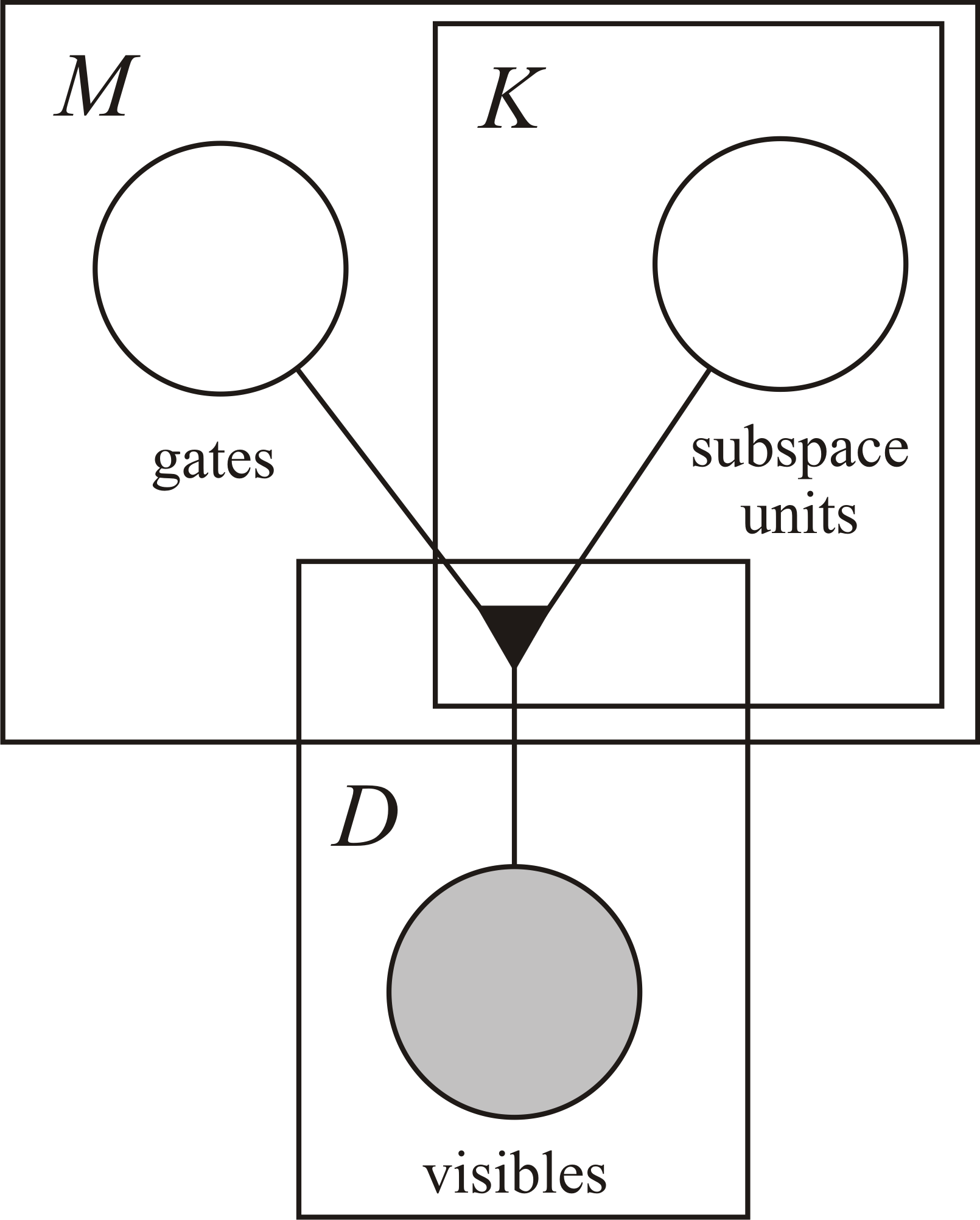
Figure 1: A graphical representation of the subspaceRBM. The triangular symbol represents a third-order multiplicative interaction.

We can get some insight into the role of the subspace hidden variables by considering the conditional distribution over $\mathbf{x}$ with $\mathbf{S}$ marginalized out:

$$p(\mathbf{x}|\mathbf{h})\propto\mathrm{exp}(\sum_{i}b_{i}x_{i}+\sum_{j}c_{j}h_{j})\prod_{j}\prod_{k}\Big{(}1+\mathrm{exp}\big{(}h_{j}(\sum_{i}W_{ijk}x_{i}+d_{jk})\big{)}\Big{)}.$$ (5)

It turns out that marginalizing out $\mathbf{S}$ entails the visible variables being conditionally dependent. Hence the subspace hidden variables model the covariance of the visible variables.

3 Learning

In training, we take advantage of the equations (2), (3), and (4) to formulate an efficient three-phase block-Gibbs sampling from the subspaceRBM. First, for given data, we sample gate units from $p(\mathbf{h}|\mathbf{x})$ with $\mathbf{S}$ marginalized out. Then, given both $\mathbf{x}$ and $\mathbf{h}$, we can sample subspace variables from $p(\mathbf{S}|\mathbf{x},\mathbf{h})$. Eventually, the data can be sampled from $p(\mathbf{x}|\mathbf{h},\mathbf{S})$.

We update the parameters of the subspaceRBM using contrastive divergence-like learning procedure. For this purpose we need to calculate the gradient of the log-likelihood function. The log-likelihood gradient takes the form of a difference between two expectations, namely, over the probability distribution with clamped data, and over the joint probability distribution of visible and hidden variables. Analogously to the standard RBM, both the expectations are approximated by samples drawn from the three-phase block-Gibbs sampling procedure.

4 Related works

The standard RBM can reflect only the second-order multiplicative interactions. However, in many real-life situations, higher-order interactions must be included if we want our model to be effective enough. Moreover, often the second-order interactions themselves might represent little or no useful information. In the literature there were several propositions of how to extend the RBM to the higher-order Boltzmann machines. One such proposal is a third-order multiplicative interaction of two visible binary units $x_{i}$, $x_{i^{\prime}}$ and one hidden binary unit $h_{j}$ (Hinton, 2010; Ranzato et al., 2010), which can be used to learn a representation robust to spatial transformations (Memisevic and Hinton, 2010). Along this line of thinking, our model is the third-order Boltzmann machine but with different multiplicative interactions of one visible unit and two kinds of hidden units.

The proposed model is closely related to the subspace spike-and-slab RBM (subspace-ssRBM) (Courville et al., 2013) where there are two kinds of hidden variables, namely, spike is a binary variable and slab is a real-valued variable. However, in our approach both the spike and slab variables are discrete. Additionally, in the subspaceRBM the hidden units $\mathbf{h}$ behave as gates to subspace variables rather than spikes as in ssRBM.

Similarly to our approach, gating units were proposed in the Point-wise Gated Boltzmann Machine (PGBM) (Sohn et al., 2013) where chosen units were responsible for switching on subsets of hidden units. The subspaceRBM is based on an analogous idea but it uses sigmoid units only whereas PGBM utilizes both sigmoid and softmax units.

Our model can be also related to RBM forests (Larochelle et al., 2010). The RBM forests assume each hidden unit to be encoded by a complete binary tree. In our approach each gate unit is encoded by subspace units. Therefore, the subspaceRBM can be seen as a RBM forest but with flatter hierarchy of hidden units and hence easier learning and inference.

Lastly, the subspaceRBM but with the softmax hidden units $\mathbf{h}$ turns to be the implicit mixture of RBMs (imRBM) (Nair and Hinton, 2008). However, in our model the gate units can be seen as pooling features while in the imRBM they determine only one subset of subspace features to be activated. The subspaceRBM brings an important benefit over the imRBM because it allows the subspaceRBM to relfect multiple factors in data.

5 Experiment

We performed the experiment using MNIST image corpora with different number of training images (10, 100, and 1000 per digit, i.e., $N\in\{100,1000,10000\}$). Additionally, the validation set of 10,000 and test set of 10,000 images were used. We compared the subspaceRBM with the RBM for the number of gate units equal $M=500$ and different number of subspace units $K\in\{3,5,7\}$, measuring reconstruction error, classification error, and mean number of active gate units. For classification the logistic regression was fed up with the probabilities of gate units, $p(h_{j}=1|\mathbf{x})$, as inputs. The learning rate was set to $0.01$ and minibatch of size $10$ was used. The number of iterations over the training set was determined using early stopping according to the validation set reconstruction error, with a look ahead of 10 iterations.

Results and Discussion.

In Table 1 test reconstruction error is presented, and in Table 3 – test classification error. A random subset of subspace features is shown in Figure 2. We notice that application of subspace units is beneficial for better reconstruction capabilities (see Table 1). In the case of classification it is advantageous to use subspaceRBM in the case of small sample size regime (for $N$ equal 100 and 1000) with smaller number of subspace units. However, this result is rather not surprising because for over-complete representations simpler classifiers work better. On the other hand, for the small sample size there is a big threat of overfitting. Introducing subspace units to the hidden layer restricts the variability of the representation and thus preventing from learning noise in data. In the case of classification for larger number of observations, the best results were obtained for $K$ equal $5$ and $7$. This result suggests that indeed the subspace units lead to more robust features.

Table 1: Test reconstruction error for different settings of the RBM and the subspaceRBM evaluated on subsets of MNIST. The best results are in bold.

	Reconstruction error
Model	N=100	N=1000	N=10000
RBM $M=500$	4.80	3.27	2.68
subspaceRBM $M=500$, $K=3$	4.56	3.01	2.57
subspaceRBM $M=500$, $K=5$	4.52	3.02	2.58
subspaceRBM $M=500$, $K=7$	4.68	3.05	2.50

Table 2: Test classification error for the RBM and different settings of the subspaceRBM evaluated on subsets of MNIST. The best results are in bold.

	Classification error [$\%$]
Model	N=100	N=1000	N=10000
RBM $M=500$	23.37	8.56	3.75
subspaceRBM $M=500$, $K=3$	23.25	8.45	3.83
subspaceRBM $M=500$, $K=5$	24.04	8.24	3.67
subspaceRBM $M=500$, $K=7$	25.64	8.78	3.64

Table 3: Number of active units for the RBM and different settings of the subspaceRBM evaluated on subsets of MNIST. The best results are in bold.

	Number of active units
Model	N=100	N=1000	N=10000
RBM $M=500$	78	68	54
subspaceRBM $M=500$, $K=3$	82	112	49
subspaceRBM $M=500$, $K=5$	74	88	78
subspaceRBM $M=500$, $K=7$	46	72	64

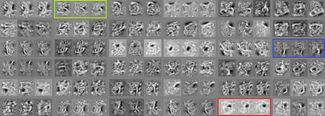
Figure 2: Random subset of subspace features for $N=10000$ and the subspaceRBM with $M=500$ and $K=3$. Exemplary three groups of filters are outlined in red, blue and green which evidently tend to learn similar pattern with offsets in position, curvature or rotation.

6 Conclusion

In this paper, we have proposed an extension of the RBM by introducing subspace hidden units. The formulated model can be seen as the third-order Boltzmann machine with third-order multiplicative interactions. We have showed that the subspaceRBM does not reduce to a vanilla version of the RBM, see equation (5), and the subspace units incorporate a manner of modelling covariance of input variables. The carried-out experiments have revealed the supremacy of the proposed model over the RBM in terms of reconstruction error; in the case of classification error – only for small sample size.

References

- Bengio et al. (2013) Yoshua Bengio, Aaron Courville, and Pascal Vincent. Representation Learning: A Review and New Perspectives. Pattern Analysis and Machine Intelligence, IEEE Transactions on, 35(8):1798–1828, Aug 2013. ISSN 0162-8828. 10.1109/TPAMI.2013.50.
- Courville et al. (2013) Aaron Courville, Guillaume Desjardins, James Bergstra, and Yoshua Bengio. The Spike-and-Slab RBM and Extensions to Discrete and Sparse Data Distributions. IEEE Transactions on Pattern Analysis and Machine Intelligence, 2013. 10.1109/TPAMI.2013.238.
- Hinton (2002) Geoffrey E Hinton. Training products of experts by minimizing contrastive divergence. Neural computation, 14(8):1771–1800, 2002.
- Hinton (2010) Geoffrey E Hinton. Learning to represent visual input. Philosophical Transactions of the Royal Society B: Biological Sciences, 365(1537):177–184, 2010.
- Larochelle et al. (2010) Hugo Larochelle, Yoshua Bengio, and Joseph Turian. Tractable multivariate binary density estimation and the restricted Boltzmann forest. Neural computation, 22(9):2285–2307, 2010.
- Memisevic and Hinton (2010) Roland Memisevic and Geoffrey E Hinton. Learning to represent spatial transformations with factored higher-order Boltzmann machines. Neural Computation, 22(6):1473–1492, 2010.
- Nair and Hinton (2008) Vinod Nair and Geoffrey E Hinton. Implicit Mixtures of Restricted Boltzmann Machines. In NIPS, volume 21, pages 1145–1152, 2008.
- Ranzato et al. (2010) Marc’Aurelio Ranzato, Alex Krizhevsky, Geoffrey E Hinton, et al. Factored 3-way restricted boltzmann machines for modeling natural images. In International Conference on Artificial Intelligence and Statistics, pages 621–628, 2010.
- Sejnowski (1986) Terrence J Sejnowski. Higher-order Boltzmann machines. In AIP Conference Proceedings, volume 151, pages 398–403, 1986.
- Sohn et al. (2013) Kihyuk Sohn, Guanyu Zhou, Chansoo Lee, and Honglak Lee. Learning and Selecting Features Jointly with Point-wise Gated Boltzmann Machines. In Proceedings of The 30th International Conference on Machine Learning, pages 217–225, 2013.