Data Assimilation by Artificial Neural Networks for an Atmospheric General Circulation Model: Conventional Observation

Abstract

This paper presents an approach for employing an artificial neural network (NN) to emulate an ensemble Kalman filter (EnKF) as a method of data assimilation. The assimilation methods are tested in the Simplified Parameterizations PrimitivE-Equation Dynamics (SPEEDY) model, an atmospheric general circulation model (AGCM), using synthetic observational data simulating localization of balloon soundings. For the data assimilation scheme, a supervised NN, the multilayer perceptron (MLP-NN), is applied. The MLP-NN is able to emulate the analysis from the local ensemble transform Kalman filter (LETKF). After the training process, the method using the MLP-NN is seen as a function of data assimilation. The NN was trained with data from first three months of 1982, 1983, and 1984. A hind-casting experiment for the 1985 data assimilation cycle using MLP-NN was performed with synthetic observations for January 1985. The numerical results demonstrate the effectiveness of the NN technique for atmospheric data assimilation. The results of the NN analyses are very close to the results from the LETKF analyses, the differences of the monthly average of absolute temperature analyses is of order $10^{-2}$. The simulations show that the major advantage of using the MLP-NN is better computational performance, since the analyses have similar quality. The CPU-time cycle assimilation with MLP-NN is $90$ times faster than cycle assimilation with LETKF for the numerical experiment.

1 Introduction

For operating systems in weather forecasting, one of the challenges is to obtain the most appropriate initial conditions to ensure the best prediction from a physical-mathematical model that represents the evolution of a physical system. Performing a smooth melding of data from observations and model predictions carries out a set of procedures to determine the best initial condition. Atmospheric observed data are used to create meteorological fields over some spatial and/or temporal domain. Data assimilation occurs when the observations and the dynamic model are combined.

The analysis for the time evolution of the atmospheric flow is based on observational data and a model of the physical system, with some background information on initial condition. The analysis is useful in itself as a description of the physical system, but it can be used as an initial state for the further time evolution of the system [Hólm (2008)].

Several techniques have been developed to identify the initial condition for numerical weather prediction (NWP). These techniques are applied in models of atmospheric and oceanic dynamics, environmental and hydrological prediction, and ionosphere dynamics. The Kalman filter (KF) [Kalman (1960)] is one strategy to estimate an appropriate initial condition. Another strategy is to find a probability density function associated with the initial condition, characterizing the Bayesian approaches [Daley (1991), Lorenc (1986)]. The ensemble Kalman filter (EnKF) [Evensen (1994), Houtekamer and Mitchell (1998)] and particle filter (PF) [Doucet et al. (2002), Andrieu and Doucet (2002)], are Bayesian techniques.

These modern techniques represent a computational challenge, even with the use of parallel computing with thousands of processors. Indeed, the challenge is the computational cost because we are moving to higher resolution models and an exponential growth in the amount of observational data. The algorithms are constantly updated to improve their performance. One example is the version of the EnKF restricted to small areas (local): the local ensemble Kalman filter (LEKF) [Ott, et al. (2004)]. The computational challenge to the techniques of data assimilation, lies in the size of matrices involved in operational NWP models, currently running under order of millions of equations (equivalent to full matrix elements of the order of $10^{12}$).

The application of Artificial Neural Networks (NN) was suggested as a possible technique for data assimilation by [Hsieh and Tang (1998)], [Liaqat et al. (2003)], and [Tang et al. (2001)]. However, [Nowosad et al. (2000)] (see also [Vijaykumar et al. (2002), Campos Velho et al. (2002)]) employed the first implementation of an NN as an approach for data assimilation, with independent development from the cited authors; they used an NN over all spatial domain. Later, this approach was improved by [Harter and Campos Velho (2005)] and [Harter and Campos Velho (2008)], they analyzed the performance of two feed-forward NN (multilayer perceptron and radial basis function), and two recurrent NN (Elman and Jordan) (see [Haykin (2001), Haykin (2007)]). [Harter and Campos Velho (2008)] introduced a modification on the NN application, in which the analysis was obtained at each grid point, instead of at all points of the domain. The modification greatly reduced the dimension of the the computational processing. Continuing the investigations, [Furtado (2008)] evaluated the performance of an NN to emulate the particle filter and the variational method for data assimilation applied to Lorenz chaotic system. The NN technique was successful for all experiments.

The use of the NN in data assimilation approach does not address error estimation. In these experiments, the NN were applied to mimic other data assimilation methods. The main advantage to using NN is the speed-up of the data assimilation process. Methods using NN have shown consistent results with implementation in the simple and low-order models.

This paper presents the approach based on using NN to emulate an EnKF version as a method of data assimilation. The NN are applied to a nonlinear dynamical system, an atmospheric general circulation model (AGCM). The AGCM used, is the Simplified Parameterizations PrimitivE-Equation Dynamics (SPEEDY) model. The method is tested with synthetic conventional data, simulating measurements from surface stations (data at each 6 hours on a day) and upper-air soundings (data at each 12 hours on a day). The application of NN produces a significant reduction for the computational effort compared to LETKF. The goal to use the NN approach is to achieve a better computational performance with similar quality for the prediction, i.e., an computational efficient process of atmospheric data assimilation (the analysis).

The technique uses NN to implement the function:

$$x^{a}=F_{NN}(y^{o},x^{f})$$ (1)

where $F_{NN}$ is the data assimilation process, $y^{o}$ are the observations, $x^{f}$ is a model forecast (simulated), often called the first guess, and $x^{a}$ is the analysis field with innovation that represents the correction to the model.

Generally, the observational data used in operational data assimilation are conventional data and satellite data. The conventional data include surface observations and upper-air observations, such as balloon soundings. Global operational satellite data are taken and processed in real time to all Earth surface. Though small in number, the conventional data are very important in the meteorological data assimilation. Then, we apply that synthetic data type in our experiment.

The experiment was conducted using the SPEEDY model [Bourke (1974), Held and Suarez (1994)], which is a 3D global atmospheric model, with simplified physics parameterization by [Molteni (2003)]. The spatial resolution considered is T30L7 for the spectral method. The grid of synthetic observations seeks to reproduce the stations of World Meteorological Organization (WMO) of rawinsonde observations. This spatial grid points are employed in this numerical experiment. Here, a set of NN multilayer perceptron (MLP) [see [Haykin (2001)]] is employed to emulate the LETKF. The LETKF technique was used as the reference analysis. More information about LETKF can be obtained from [Bishop et al.(2001), Hunt et al. (2007)] and [Miyoshi and Yamane (2007)].

Our paper shows that the analysis computed by the NN has the same quality as the analysis produced by LETKF, which was analyzed by expert meteorologists, see [Miyoshi (2005)] and [Kalnay (2003)].

2 Methodology

2.1 Artificial Neural Network (NN)

An NN is a computational system with parallel and distributed processing that has the ability to learn and store experimental knowledge. An NN is composed of simple processing units that compute certain mathematical functions (usually nonlinear). An NN consists of interconnected artificial neurons or nodes, which are inspired by biological neurons and their behaviour. The neurons are connected to others to form a NN, which is used to model relationships between artificial neurons.

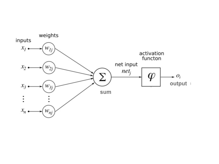
Figure 1: Artificial Neural Neuron components.

Each artificial neuron is constituted by one or more inputs and one output. The neuron process is nonlinear, parallel, local, and adaptable. Each neuron has a function to define outputs, associated with a learning rule. The neuron connection stores a nonlinear weighted sum, called a weight. In NN processing, the inputs are multiplied by weights; these results summarized then go through the activation function. This function activates or inhibits the next neuron. Mathematically, we can describe the $i^{th}$ input with the following form:

$$\begin{array}[]{ll}\mbox{input summation:}&u_{i}=\sum^{p}_{j=1}{w_{ij}x_{j}}\\ \mbox{neuron output:}&y_{i}=\varphi(u_{i})\end{array}$$ (2)

where $x_{1},x_{1},.\cdots,x_{p}$ are the inputs; $w_{i1},\cdots,w_{ip}$ are the synaptic weights; $u_{i}$ is the output of linear combination; $\varphi(\cdot)$ is the activation function, and $y_{i}$ is the $ith$ neuron output, $p$ is number of neurons (Fig. 1).

A feed-forward network, which processes in one direction from input to output, it has a layered structure. The first layer of an NN is called the input layer, the intermediary layers are called hidden layers, and the last layer is called the output layer. The number of layers and the quantity of neurons in each is determined by the nature of the problem. In most applications, a feed-forward NN with a single layer of hidden units is used with a sigmoid activation function, such as the hyperbolic tangent function for the units

$$\mbox{hyperbolic tangent function}:$$

$$\varphi(v)=\frac{1-\exp(-av)}{1+\exp(-av)}\leavevmode\nobreak\ .$$ (3)

There is two distinct phases in using an NN: the training phase (learning process) and the run phase (activation or generalization). The training phase of the NN consists of an iterative process for adjusting the weights for the best performance of the NN in establishing the mapping of input and target vector pairs. The learning algorithm is the set of procedures for adjusting the weights. The single pass through the entire training set in one process in called an epoch. Testing of the verification set follows each epoch, the iterative process continues or stops after verification of defined criteria, which can be minimum error of mapping or number of epochs. Once the NN is trained (the process is stopped) , the weights are fixed, and the NN is ready to receive new inputs (different from training inputs) for which it calculates the corresponding outputs. This phase is called the generalization. Each connection (after training) has an associated weight value that stores the knowledge represented in the experimental problem and considers the input received by each neuron of that NN.

Neural network designs or architectures are dependent upon the learning strategy adopted [see Haykin [Haykin (2001)]]. The multilayer perceptron (MLP) is the NN architecture used in this study; which the interconnections between the inputs and the output layer have at least one intermediate layer of neurons, a hidden layer [[Gardner and Dorling (1998)], [Haykin (2007)]].

Neural Networks can solve nonlinear problems if nonlinear activation functions are used for the hidden and/or the output layers. The use of units with nonlinear activation functions generalizes the delta rule. Developed by [Widrow and Hoff (1960)], the delta rule is a version of the least mean square (LMS) method. For a given input vector $x$, the output vector $x^{a}_{NN}$ is compared to the target answer $x^{a}_{ref}$. If the difference is near zero, no learning takes place; if the difference is not near zero, the weights are adjusted to reduce this difference. The purpose is to minimize the output errors by adjusting the NN weights, $w_{ij}$, using the delta rule algorithm, summarized as follows:

1. Compute the error function $E(w_{ij})$, defining the distance between the target and the result: $E(w_{ij})\equiv[x^{a}_{ref}-x^{a}_{NN}]^{2}$

2. Compute the gradient of the error function $\partial{E(w_{ij})}/\partial{w_{ij}}=\delta_{j}y_{i}$, defining which direction should move in weight space to reduce the error, and $\delta_{j}\equiv(x^{a}_{ref}-x^{a}_{NN})\varphi^{\prime}(v)$.

3. Select the learning rate $\eta$ which specifies the step size taken in the weight space of update equation;

4. Update the weight for the epoch $k$: $w_{ij}^{k}=w_{ij}^{k-1}+\Delta w_{ij}$, where $\Delta w_{ij}=-\eta{E(w_{ij})}/\partial{w_{ij}}$. One epoch or training step is a set of update weights for all training patterns.

5. Repeat step[4] until the NN error function, reach the required precision. This precision is a defined parameter that stops the iterative process.

The overall idea is to treat the NN as a function of the weights $w_{ij}$ (Eq. 2), instead of the inputs. The goal is to minimize the error between the actual output $y_{i}$ (or $x^{a}_{NN}$) and the target output ($d_{i}$) (or $x^{a}_{ref}$) of the training data. For each (input/output) training pair, the delta rule determines the direction you need to be adjusted to reduce the error. By taking short steps, we can find the best direction for the entire training. To consider a set of (input and target) pairs of vectors $\{(x_{0},d_{0}),\ (x_{1},d_{2}),\cdots,(x_{N},d_{N})\}^{T}$, where $N$ is the number of patterns (input elements), and one output vector $y=[y_{0},y_{1},y_{2},\cdots,y_{N}]^{T}$, a MLP performs a complex mapping $y=\varphi(w,x)$ parameterized by the synaptic weights $w$, and the functions $\varphi(\cdot)$ that provide the activation for the neuron.

The set of procedures to adjust the weights is the learning algorithm. back-propagation, a well-known learning scheme, is generally used for the MLP training (it performs the delta rule (the algorithm above). Back-propagation training is a supervised learning., e.g. the adjustments to the weights are conducted by back propagating, or considering the difference between the NN calculated output and the target output (considered the supervisor).

[Hsieh (2009)], and [Haupt et al. (2009)] reviewed applications of NN in environmental science including in atmospheric sciences. They reviewed some NN concepts and some applications, they presented others estimation methods and its applications. The NN applications, generally, are on function approximation of modeling of nonlinear transfer functions, and pattern classifications. [Gardner and Dorling (1998)] included brief introductions of MLP and the back-propagation algorithm; they showed a review for applications in the atmospheric sciences, looking at prediction of air-quality, surface ozone concentration, dioxide concentrations, severe weather, etc., and pattern classifications applications in remote sensing data to obtain distinction between clouds and ice or snow. Applications on classification of atmospheric circulation patterns, land cover and convergence lines from radar imagery, and classification of remote sensing data using NN, were also presented in Hsieh (2009) and Haupt et al. (2009).

2.2 The SPEEDY Model

The SPEEDY computer code is an AGCM developed to study global-scale dynamics and to test new approaches for NWP. The dynamic variables for the primitive meteorological equations are integrated by the spectral method in the horizontal at each vertical level (see [Bourke (1974), Held and Suarez (1994)]).

The model has a simplified set of physical parameterization schemes that are similar to realistic weather forecasting numerical models. The goal of this model is to obtain computational efficiency while maintaining characteristics similar to the state-of-the-art AGCM with complex physics parameterization [Miyoshi (2005)].

According to [Molteni (2003)], the SPEEDY model simulates the general structure of global atmospheric circulation fairly well, and some aspects of the systematic errors are similar to many errors in the operational AGCMs. The package is based on the physical parameterizations adopted in more complex schemes of the AGCM, such as convection (simplified diagram of mass flow), large-scale condensation, clouds, short-wave radiation (two spectral bands), long–wave radiation (four spectral waves), surface fluxes of momentum, energy (aerodynamic formula), and vertical diffusion. Details of the simplified physical parameterization scheme can be found in [Molteni (2003)].

The boundary conditions of the SPEEDY model includes topographic height and land-sea mask, which are constant. Sea surface temperature (SST), sea ice fraction, surface temperature in the top soil layer, moisture in the top soil layer, the root-zone layer, snow depth, all of which are specified by monthly means. Bare-surface albedo, and fraction of land-surface covered by vegetation, are specified by annual-mean fields. The lower boundary conditions such as SST are obtained from the ECMWF’s reanalysis in the period 1981-90. The incoming solar radiation flux and the boundary conditions (SST, etc.), are updated daily. The SPEEDY model is a hydrostatic model in sigma coordinates, [Bourke (1974)] also describes the vorticity-divergence transformation scheme.

The SPEEDY model is global with spectral resolution T30L7 (horizontal truncation of 30 numbers of waves and seven levels), corresponding to a regular grid with 96 zonal points (longitude), 48 meridian points (latitude), and 7 vertical pressures levels (100, 200, 300, 500, 700, 850, and 925 hPa). The prognostic variables for the model input and output are the absolute temperature ($T$), surface pressure ($p_{s}$), zonal wind component ($u$), meridional wind component ($v$), and an additional variable and specific humidity ($q$).

2.3 Brief Description on Local Ensemble Transform Kalman Filter

The analysis is the best estimate of the state of the system based on the optimizing criteria and error estimates. The probabilistic state space formulation and the requirement for updating information when new observations are encountered are ideally suited to the Bayesian approach. The Bayesian approach is a set of efficient and flexible Monte Carlo methods for solving the optimal filtering problem. Here, one attempts to construct the posterior probability density function (pdf) of the state using all available information, including the set of received observations. Since this pdf embodies all available statistical information, it may be considered as a complete solution to the estimation problem.

In the field of data assimilation, there are only few contributions in sequential estimation (EnKF or PF filters). The EnKF was first proposed by [Evensen (1994)] and was developed by [Burgers et al.(1998)] and [Evensen (2003)]. It is related to particle filters in the context that a particle is identified as an ensemble member. EnKF is a sequential method, which means that the model is integrated forward in time and whenever observations are available; these EnKF results are used to reinitialise the model before the integration continues. The EnKF originated as a version of the Extended Kalman Filter (EKF) [[Kalman and Bucy (1961)]]. The classical KF method by [Kalman (1960)] is optimal in the sense of minimizing the variance only for linear systems and Gaussian statistics. Analysis perturbations are added to run the ensemble forecasts. [Miyoshi and Yamane (2007)] added Gaussian white noise to run the same forecast for each member of the ensemble in LETKF. The EnKF is a Monte Carlo integration that governs the evolution of the pdf, which describes the a priori state, the forecast and error statistics. In the analysis step, each ensemble member is updated according to the KF scheme and replaces the covariance matrix by the sampled covariance computed from the ensemble forecasts.

[Houtekamer and Mitchell (1998)] first applied the EnKF to an atmospheric system. They applied an ensemble of model states to represent the statistical model error. The scheme of analysis acts directly on the ensemble of model states when observations are assimilated. The ensemble of analysis is obtained by assimilation for each member of the reference model. Several methods have been developed to represent the modeling error covariance matrix for the analysis applying the EnKF approach; the local ensemble transform Kalman filter (LETKF) is one of them. [Hunt et al. (2007)] proposed the LETKF scheme as an efficient upgrade of the local ensemble Kalman filter (LEKF). The LEKF algorithm creates a close relationship between local dimensionality, error growth, and skill of the ensemble to capture the space of forecast uncertainties, formulated with the EnKF scheme (e.g., [Whitaker and Hamill (2002)]). In addition, [Kalnay (2003)] describes the theoretical foundation of the operational practice of using small ensembles, for predicting the evolution of uncertainties in high-dimension operational NWP models.

The LETKF scheme is a model-independent algorithm to estimate the state of a large spatial temporal chaotic system [Ott, et al. (2004)]. The term ”local” refers to an important feature of the scheme: it solves the Kalman filter equations locally in model grid space. a kind of ensemble square root filtering [Miyoshi (2005)],[Whitaker and Hamill (2002)], in which the analysis ensemble members are constructed by a linear combination of the forecast ensemble members. The ensemble transform matrix, composed of the weights of the linear combination, is computed for each local subset of the state vector independently, which allows essentially parallel computations. The local subset depends on the error covariance localization [Miyoshi and Kunii (2012)]. Typically a local subset of the state vector contains all variables at a grid point. The LETKF scheme first separates a global grid vector into local patch vectors with observations.

The basic idea of LETKF is to perform analysis at each grid point simultaneously using the state variables and all observations in the region centred at given grid point.The local strategy separates groups of neighbouring observations around a central point for a given region of the grid model. Each grid point has a local patch; the number of local vectors is the same as the number of global grid points [Miyoshi and Yamane (2007)].

The algorithm of EnKF follows the sequential assimilation steps of classical Kalman filter, but it calculates the error covariance matrices as described bellow:

Each member of the ensemble gets its forecast

$$\{x^{f}_{n-1}\}^{(i)}\ :\ i=1,2,3,\cdots,k,$$

where $k$ is the total members at time $t_{n}$, to estimate the state vector $\bar{x}^{f}$ of the reference model. The ensemble is used to calculate the mean of forecasting $(\bar{x}^{f})$

$$\bar{x}^{f}\equiv k^{-1}\sum^{k}_{i=1}\{x^{f}\}^{(i)}\leavevmode\nobreak\ .$$ (4)

Therefore, the model error covariance matrix is:

$$P^{f}=(k-1)^{-1}\sum^{k}_{i=1}{(\{x^{f}\}^{(i)}-\bar{x}^{f})(\{x^{f}\}^{(i)}-\bar{x}^{f})^{T}}.$$ (5)

The analysis must determine a state estimate and the covariance error matrix $P^{a}$, but also an ensemble with the appropriate sample analyses mean $\{x^{a}_{n-1}\}^{(i)}\ :\ i=1,2,3,\cdots,k,$

$$\bar{x}^{a}\equiv k^{-1}\sum^{k}_{i=1}\{x^{a}\}^{(i)}\leavevmode\nobreak\$$ (6)

$$P^{a}=(k-1)^{-1}\sum^{k}_{i=1}{(\{x^{a}\}^{(i)}-\bar{x}^{a})(\{x^{a}\}^{(i)}-\bar{x}^{a})^{T}}.$$ (7)

Important properties of the LETKF include the following:

• Solve the estimation problem independently at each local region;

• Update the estimate of the current state and also its uncertainty;

• Assimilate all data at once;

• Can deal with observations from the nonlinear functions of the state vector;

• Interpolate observations in time as well as in space (full 4D assimilation scheme);

• Set local region size and ensemble size (free parameters only);

• Be model independent (no adjoints!);

• Can estimate model parameters errors as well as initial conditions.

The LETKF code has been applied to a low-dimensional AGCM SPEEDY model [Miyoshi (2005)], a realistic model according [Szunyogh et al. (2007)]. The LETKF scheme was also applied in: the AGCM for the Earth Simulator by [Miyoshi and Yamane (2007)] and the Japan Meteorological Agency operational global and mesoscale models by[Miyoshi et al. (2010)]; The Regional Ocean modeling System by [Shchepetkin and McWilliams (2005)]; the global ocean model known as the Geophysical Fluid Dynamics Laboratory (GFDL) by [Penny (2011)]; and GFDL Mars AGCM by [Greybush (2005)].

3 MLP-NN in assimilation for SPEEDY model

The NN configuration for this experiment is a set of multilayer perceptrons, hereafter referred to as MLP-NN, with the following characteristics:

• Two input nodes, one node for the meteorological observation vector and the other for the 6-hours forecast model vector. The vectors values represent individual grid points for a single variable with a correspondent observation value.

• One output node for the analysis vector results. In the training algorithm, the MLP-NN computes the output and compared it with the analysis vector of LETKF results (the target data, but not a node for the NN). The vectors represent individual analysis values for one grid point.

• One hidden layer with eleven neurons.

• The hyperbolic tangent (Eq. 2.1) as the activation function (to guarantee the nonlinearity for results).

• Learning rate $\eta$ is $0.001$

• Training stops when the error reaches $10^{-5}$ or after 5000 epochs, which criterion first occurs.

On the present paper, the NN configuration (number of layers, nodes per layer, activation function, and learning rate parameter) was defined by empirical tests. Care must be taken in specifying the number of neurons. Too many can lead the NN to memorize the training data (over fitting), instead of extracting the general features that allow the generalization. Too few neurons may force the NN to spend too much time trying to find an optimal representation and thus wasting valuable computation time. The automatic configuration of NN is a recent topic of a discussion by [Sambattit et al. (2012)].

One strategy used to collect data and to accelerate the processing of the MLP-NN training was to divide the entire globe into six regions: for the Northern Hemisphere, $90^{o}$ N and three longitudinal regions of $120^{o}$ each; for the Southern Hemisphere, $90^{o}$ S and three longitudinal regions of $120^{o}$ each. This division is based on the size of the regions, but the number of observations is distinct, as illustrated by Fig. 2. This regional division is applied only for the MLP-NN; the LETKF procedures are not modified.

The MLP-NN were developed with a set of thirty NN (six regions with five prognostic variables ($p_{s},$ u, v, T, and q). One MLP-NN with characteristics described above, was designed for each meteorological variable of the SPEEDY model and each region. Each MLP has two inputs (model and observation vectors), one output neuron which is the analysis vector, and eleven neurons in a hidden layer. The activation function used to ensure nonlinearity of the problem is the hyperbolic tangent (Eq. 3), and learning rate parameter is defined to each variable set of networks, and the training scheme is the back-propagation algorithm.

The MLP-NN is designed to emulate the LETKF. Fortran90 codes for SPEEDY and LETKF [originally developed by [Miyoshi (2005)]] were adapted to create the training dataset. The upper levels and the surface covariance error matrices to run the LETKF system, as well as the SPEEDY model boundary conditions data and physical parametrizations, are the same as those used for Miyoshi’s experiments.

The initial process to run the implementation of the model assumes that it is perfect (initialization=0); and the SPEEDY model T30L7 integrated for one year of spin-up, i.e. the period required for a model to reach steady state and obtains the simulated atmosphere. The integration run for 01 January 1981 until 31 December 1981 and the result was the initial condition for SPEEDY to 01 January 1982, the date to initiate the experiment.

The output model fields, so-called ”true" model, were generated without assimilation (each 6-hours forecast of one execution is the initial condition for the next execution). The ”true" (or control) model forecasts collected for model executions without observations, considered four times per day (0000, 0600, 1200, 1800 UTC), from 01 January 1982 through 31 December 1984.

The synthetic observations were generated, reading the true SPEEDY model fields, and adding a random noise of standard deviation error from meteorological variables: surface pressure ($p_{s}$), zonal wind component ($u$), vertical wind component ($v$), absolute temperature ($T$), and specific humidity ($q$) at each grid point where is located an observations. The variables were located at all grid points of the model. An observation mask was designed, adding a positive flag at grid points where the observation should be considered, the locations chosen simulate the WMO data stations observations from radiosonde (see Fig. 2). Except for $p_{s}$ observations, the other observations are upper level with seven levels. Both assimilation schemes, LETKF and MLP-NN, use the same number of observations at the same grid point localization.

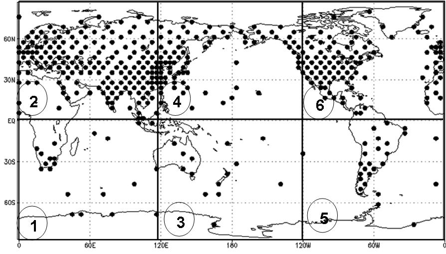
Figure 2: Observations localization in global area. The dot points represent radiosonde stations (about 415) divided in six regions.

3.1 Training Process

The training process for the experiment is conducted with forecasts obtained from the SPEEDY model and LETKF analyses for the input/target vectors. The LETKF analyses are executed with synthetic observations: upper-levels wind, temperature and humidity, and surface pressure at 0000 and 1200 UTC (at 12,035 points), and only surface observations at 0600 and 1800 UTC (at 2,075 points). These LETKF processes generated the observations and analysis vectors, and forecasts vectors for NN inputs. The analysis vector is the target for training the MPL-NN with back-propagation algorithm. The analyses and forecasts are the average of the ensemble fields.

Executions of the model with the LETKF data assimilation were made for the same period mentioned for the ”true” model: from 01 January 1982 through 31 December 1984. The ensemble forecasts of LETKF has 30 members. The ensemble average of the forecast and analyses fields, to this training process, are obtained by running SPEEDY model with the LETKF scheme.

These data are collected, initially, by dividing the globe into two regions (northern and southern hemispheres), but the computational cost was high because the training process took one day for the performance to converge. Next, the two regions were divided each into three regions, for a total of six regions. When we divided the globe into six regions, the training, for a set of NN, took about minutes. The training time is important because if the NN lose knowledge of the system, the re-training is necessary. Then, we use this division strategy to collect the thirty input vectors (observations, mean forecasts, and mean analyses) at chosen grid points by the observation mask (see above), during LETKF process. The NN training process begin after collecting the input vectors for whole period (three years).

The MLP-NN data assimilation scheme has no error covariance matrices to inform the spread of different observations. Therefore, to capture the influence of observations from the neighbouring region around a grid point, it is necessary to consider these observations. This calculation was based on the distance from the grid point related to observations inside a determined neighbourhood (initially:$\gamma=0$)

$$\hat{y}^{o}_{i\pm m,j\pm m,k\pm m}=\frac{y^{o}_{ijk}}{(6-\gamma)\,r^{2}_{ijk}}+\sum_{l=1}^{6}\alpha_{l}\frac{y^{o}_{i\pm m,j\pm m,k\pm m}}{r^{2}_{ijk}}$$ (8)

$$(m=1,2,\ldots,M)$$

$$\alpha_{l}=\left\{\begin{array}[]{ll}0&\mbox{(if there is no observation)}\\ 1&\mbox{(if there is observation, and:}\gamma_{\rm new}=\gamma_{\rm old}+1)\\ \end{array}\right.$$

where $\hat{y}^{o}$ is the weighted observation, $M$ is the number of discrete layers considered around observation, $r_{ijk}^{2}=(x_{p}-y^{o}_{i})^{2}+(y_{p}-y^{o}_{j})^{2}+(z_{p}-y^{o}_{k})^{2}$, where $(x_{p},y_{p},z_{p})$ is coordinate of the grid point, and the $(y^{o}_{i},y^{o}_{j},y^{o}_{k})$ is the coordinate of the observation, and $\gamma$ is a counter of grid points with observations around that grid point $(y^{o}_{i},y^{o}_{j},y^{o}_{k})$. If $\gamma=6$ there is no influence to be considered.

Each influence observation is a new grid observation location, hereafter referred to as pseudo-observation, which adds values to the three input vectors to NN training process. Then, the grid points to be considered in MPL-NN analysis is greater than grid points considered to LETKF analysis, although these calculations are made without interference on LETKF system.

The back-propagation algorithm stops the training process using the criteria cited at item 6 in this section, after obtaining the best set of weights; it is a function of smallest error between the MPL-NN analysis and the target analysis, (e. g. when the root mean square error between the calculated output and the input desired vector is less than $10^{-5}$) for all NN. The training process was carried out for one or two epochs for each NN. The training for a set of 30 NN took about fifteen minutes to get the fixes weights before the MLP-NN data assimilation cycle or generalization process of MLP-NN.

3.2 Generalization Process

The training was performed with combined data from January, February, and March of 1982, 1983, and 1984 and MLP-NN is able to perform an analysis similar to the LETKF analysis in generalization process.

The generalization process is indeed, the data assimilation process. The MLP-NN results a analysis field. The MLP-NN activation was entering by input values at each grid point once, with no data used in the training process. The input vectors are done at grid point where is marked with observation or pseudo-observation (Eq. 8). The procedure was the same for all NN, but one NN for each region and each prognostic variable, has different connection weights. The set of NN has one hidden layer, with the same number of neurons for all regions. The grid points are put in the global domain to make the analysis field after generalization process of MLP-NN, e.g. the activation of the set of 30 NN results a global analysis. The regional division is only for inputting each NN activation.

The MLP-NN data assimilation was performed for one-month cycle. It started at 0000 UTC 01 January 1985, generating the initial condition to SPEEDY model and running the model to get 6-hours forecast for the next execution, i.e., the 0000 UTC cycle runs MLP-NN with observations for 0000 UTC of 01 January 1985 and the 6-hours forecast from 1800 UTC of 31 December 1984l, the result of MLP-NN is the initial condition of 0000 UTC to run the SPEEDY model and its result is the forecast to 0006 UTC, which is used to the 0006 UTC cycle, and so on.

In this experiment the MLP-NN begins the activation in 01 January 1985 and generates analyses and 6 hours forecasts up through 31 January 1985.

4 Results

The input and output values of prognostic variables ($p_{s}$, u, v, T, and q) are processed on grid points for time integrations to an intermittent forecasting and analysis cycle. Two discrete layers $M=2$ around a given observation are considered: in Eq. 8.

The results show the comparison of analyses fields, generated by the MLP-NN and the LETKF data assimilation schemes, and the true model field. The global surface pressure fields (at 11 January 1985 at 1800 UTC) and differences between the analyses are shown in Fig. 3. The analyses fields and the differences between both, for 11 January 1985 at 1800 UTC at 950 hPa and 500 hPa, are also shown, for T, u, v and q meteorological global fields, in Figs. 4 - 11. These results show that the application of MLP-NN, as an assimilation system, generates analyses similar to the analyses calculated by the LETKF system. Sub-figure (d) of Figs. 4 - 11 shows that the differences between the MLP-NN and LETKF analyses are very small, we can verify the difference field of absolute temperature at 500 hPa, the differences are about $3^{o}$ degrees; or the differences field of humidity at 950 hPa, are about $0.002$.

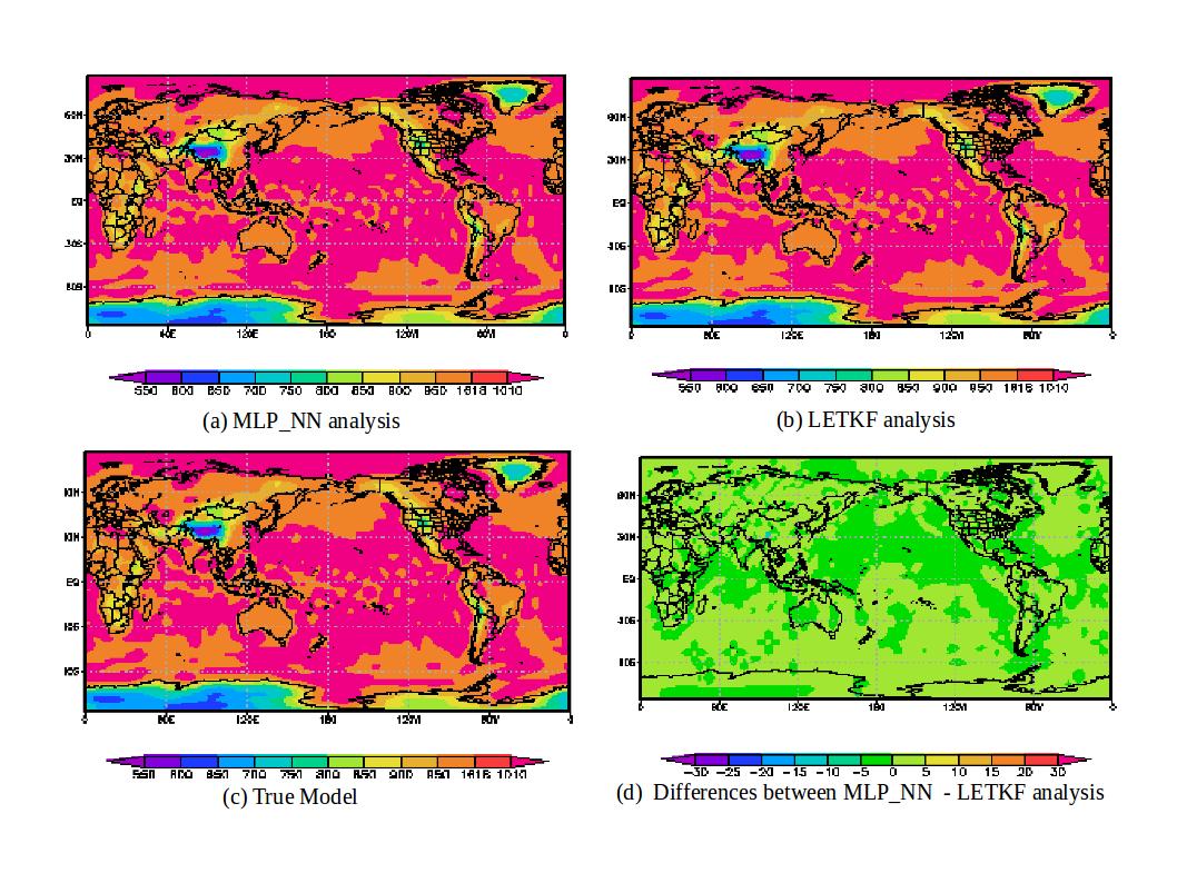
Figure 3: Surface Pressure (PS) [Pa] Fields - Jan/11/1985 at 18 UTC

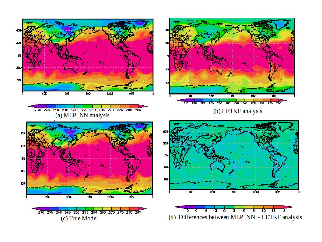
Figure 4: Absolute Temperature (T) [K] Fields at 950 hPa - Jan/11/1985 at 18 UTC

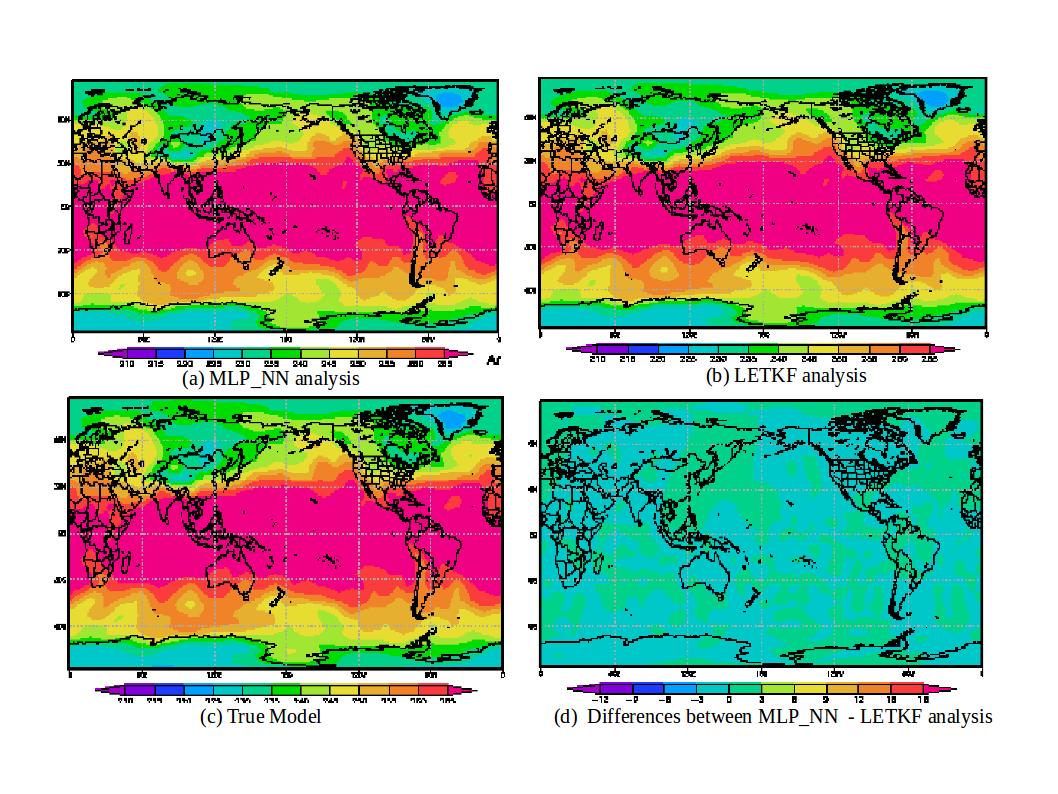
Figure 5: Absolute Temperature (T) [K] Fields at 500 hPa - Jan/11/1985 at 18 UTC

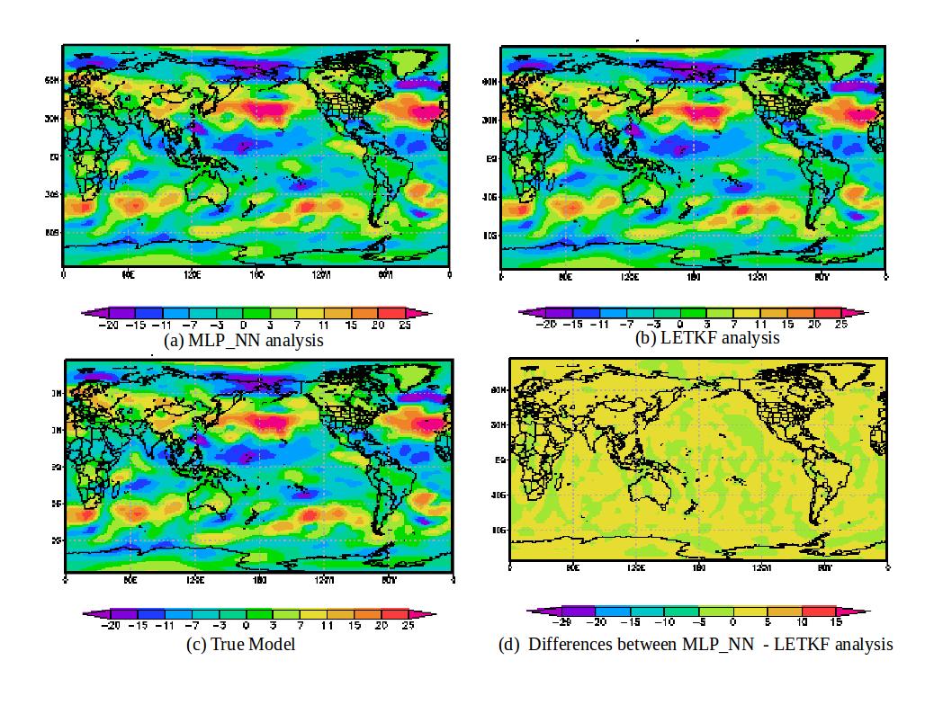
Figure 6: Zonal Wind Component (u) [m/s] Fields at 950 hPa - Jan/11/1985 at 18 UTC

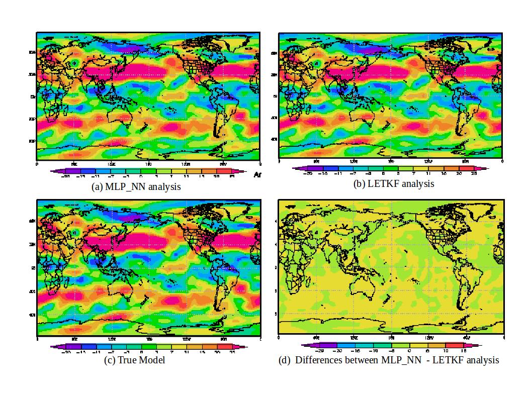
Figure 7: Zonal Wind Component (u) [m/s] Fields at 500 hPa - Jan/11/1985 at 18 UTC

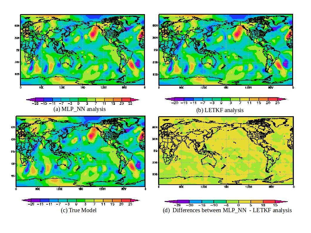
Figure 8: Meridional Wind Component (v) [m/s] Fields at 950 hPa - Jan/11/1985 at 18 UTC

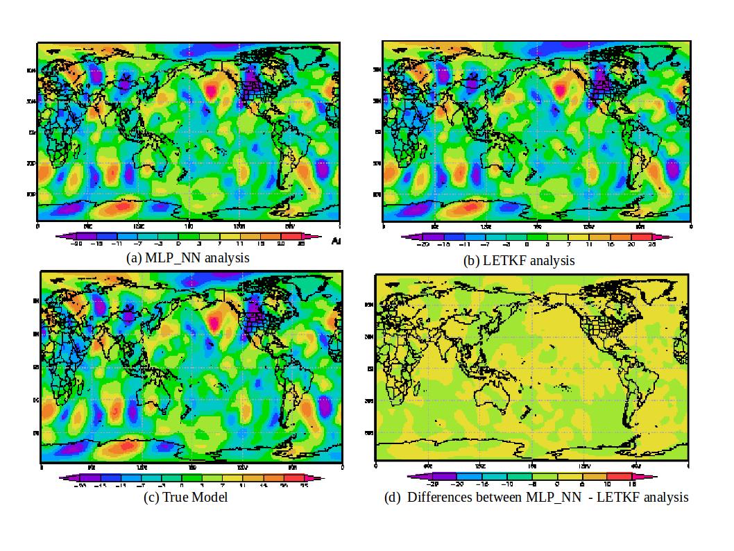
Figure 9: Meridional Wind Component (v) [m/s] Fields at 500 hPa - Jan/11/1985 at 18 UTC

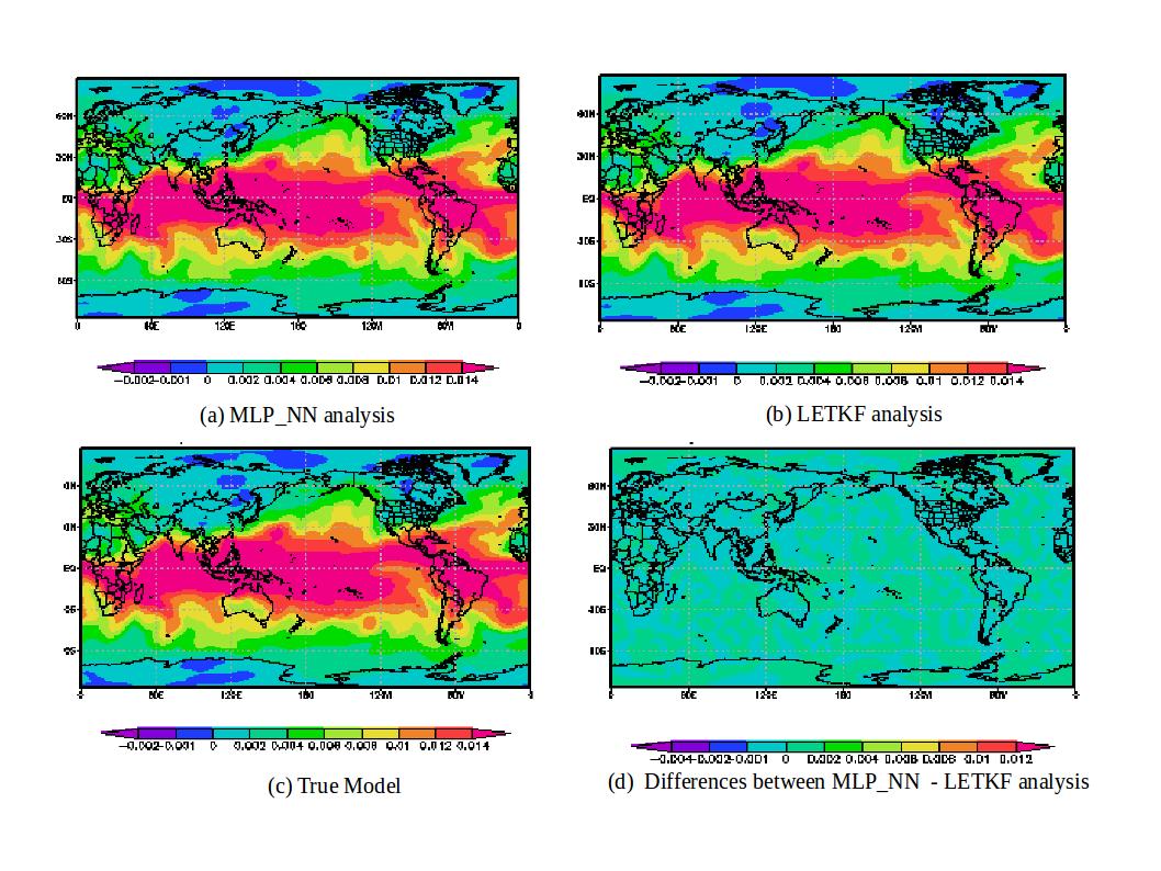
Figure 10: Specific Humidity (q) [kg/kg] Fields at 950 hPa - Jan/11/1985 at 18 UTC

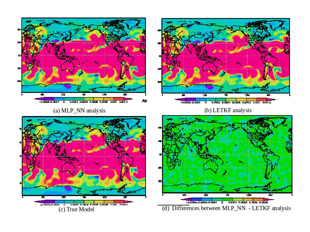
Figure 11: Specific Humidity (q) [kg/kg] Fields at 500 hPa - Jan/11/1985 at 18 UTC

Monthly mean of absolute temperature analyses fields were obtained; the differences field between the analyses (LETKF and MLP-NN) for data assimilation cycles is shown in Fig. 12. The differences are slightly larger in some regions, such as the northeast regions of North America and South America.

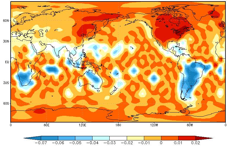
Figure 12: Differences field of the average of absolute temperature MLP-NN analysis and LETKF analysis for the assimilation cycle.

The root mean square error (RMSE) of the absolute temperature analyses to true model, are calculated by fixing a point in longitude ($87^{o}$W) for all latitude points. Fig. 13 shows the temperature RMSEs for the entire period of the assimilation cycle (January 1985). Subfigure (a) for Fig. 13 shows the RMSE of the LETKF analysis by line, and the RMSE of the MLP-NN analysis by circles; and subfigure (b) for Fig. 13 shows the differences between LETKF and MLP-NN analyses RMSE. The differences are less than $10^{-3}$.

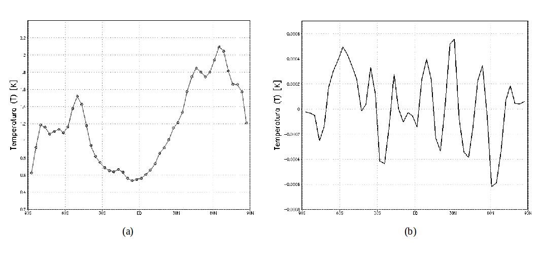
Figure 13: Meridional Root Mean Square Error for entire period of the assimilation cycles. RMSE analyses to the ”true” state, (a) the errors of the LETKF analysis (line) and the errors of MLP-NN analysis (circles) to the absolute temperature at 500 hPa, (b) the differences of RMSE analyses.

4.1 Computer Performance

Several aspects of modeling stress computational systems and push capability requirements. These aspects include increased resolution, the inclusion of improved physics processes and concurrent execution of Earth-system components - that is, coupled models (ocean circulation, and environmental prediction, for example). Often, real-time necessities define capability requirements. In data assimilation, the computational requirements become much more challenging. Observations from Earth-orbiting satellites in operational numerical prediction models are used to improve weather forecasts. However, using this amount of data increases the computational effort. As a result, there is a need for an assimilation method able to compute the initial field for the numerical model in the operational window-time to make a prediction. At present, most of the NWP centers find it difficult to assimilate all the available data because of computational costs and the cost of transferring huge amounts of data from the storage system to the main computer memory.

The data assimilation cycle has a recent forecast and the observations as the inputs for assimilation system. The latter MLP-NN system produced a analysis to initiate the actual cycle, Fig. 14 shows 112 cycles of data assimilation runs. This time simulation experiment is for (28 days) January 1985. There were 2,075 observations inserted at runs of 0600 and 1800 UTC for surface variables and 12,035 observations inserted at runs of 0000 and 1200 UTC for all upper layer variables.

The LETKF data assimilation cycle initiates, running the ensemble forecasts with the SPEEDY model and each analysis produced to each member at the latter LETKF cycle to result thirty 6-hours forecasts; the second step is to compute the average of those forecasts. After, with a set of observations and the mean forecast, the LETKF system is performed. The LETKF cycle results one analysis to each member for the ensemble, and one average field of the ensemble analyses. The MLP-NN data assimilation cycle is composed by the reading of 6-hours. forecast of SPEEDY model from latter cycle and reading the set of observations to the cycle time, the division of input vectors, the activation of MLP-NN and the assembly of output vectors to a global analysis field.

The MLP-NN runtime measurement is magenta point of Fig. 14; it initiates after reading the 6-hours. forecast of SPEEDY model from latter cycle; and the set of observations, it is the time of generalization MLP-NN with dividing forecasting/observations and with gathering global analysis. The LETKF runtime measurement is the blue point of Fig. 14; it initiates after reading the mean 6-hours forecast of SPEEDY model and the set of observations. The LETKF time include the results of 30 analyses and one mean ensemble analysis.

The comparison in Table 1 is the data assimilation cycles for the same observations points and the same model resolution to the same time simulations. LETKF and MLP-NN executions are performed independently.

Considering the total execution time of those 112 cycles simulated, the computational performance of the MLP-NN data assimilation, is better than that obtained with the LETKF approach. These results show that the computational efficiency of the NN for data assimilation to the SPEEDY model, for the adopted resolution, is 90 times faster and produces analyses of the same quality (see Table 1). Considering only the analyses execution time of those 112 data assimilation processes simulated, the computational efficiency of MLP-NN is 421 times faster than LETKF process. The Table LABEL:tab:tempos2 shows the mean execution time of each element to one cycle of: the LETKF data assimilation method (ensemble forecast and analysis) and the MLP-NN method (model forecast and analysis). The computational efficiency of one MLP-NN execution, keeps the relationship about speed-up, comparing with one LETKF execution. (421 times faster). Details for this experiment can be found in [Cintra, R. (2010)].

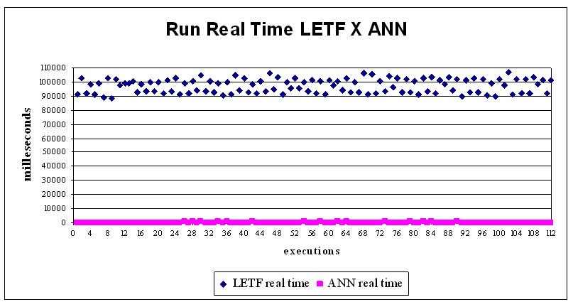
Figure 14: CPU-time for assimilation experiment: MLP-NN (magenta color), and LETKF (blue color) methods.

Table 1: Total running time of 112 cycles of complete data assimilation (analysis and forecasting)

Execution of 112 cycles	MLP-NN (hour:min:sec)	LETKF (hour:min:sec)
Analisys time	00:00:25	03:14:55
Ensemble time	00:00:00	01:05:44
Single model time	00:02:28	00:00:00
Total time	00:02:53	04:20:39

5 Conclusions

In this study, we evaluated the efficiency of the MLP-NN in an atmospheric data assimilation context. The MLP-NN is able to emulate systems for data assimilation. For the present investigation, the MLP-NN approach is used to emulate the LETKF approach, which is designed to improve the computational performance of the standard EnKF. The another experiments with the same methodology can be found in [Cintra, R. and Campos Velho, H. (2012), Cintra, R. et al. (2013)].

The NN learned the whole process of the mathematical scheme of data assimilation through training with the LETKF. The results for the MLP-NN analysis are very close to the results obtained from the LETKF data assimilation for initializing the SPEEDY model forecast, i.e., the analyses obtained with MLP-NN for the analysis field are similar to analyses computed by the LETKF, the differences between MLP-NN and LETKF analyses to surface pressure fields in hPa, for example, is about (-5 to 5) hPa. However, the computational performance of the set of thirty NN is better. The MLP-NN assimilation speed-up the LETKF scheme.

The application of the present NN data assimilation methodology is proposed at the Center for Weather Prediction and Climate Studies (Centro de Previsão de Tempo e Estudos Climáticos - CPTEC/INPE) with operational numerical global model and observations using nowadays.

6 Acknowledgements

The authors thank Dr. Takemasa Miyoshi and Prof. Dr. Eugênia Kalnay for providing computer routines for the SPEEDY model and the LETKF system. This paper is a contribution of the Brazilian National Institute of Science and Technology (INCT) for Climate Change funded by CNPq Grant Number 573797/2008-0 e FAPESP Grant Number 2008/57719-9. Author HFCV also thanks to the CNPq (Grant number 311147/2010-0).

References

- [Andrieu and Doucet (2002)] Andrieu, C. and Doucet, A.: Particle filtering for partially observed Gaussian state space models. Journal of the Roy. Statistical Society, 64(4), 827-836, 2002.
- [Bishop et al.(2001)] Bishop, H. C., Etherton, B. J. and Majumdar, S. J.: Adaptive sampling with the ensemble transform Kalman filter. part I: Theoretical aspects. Monthly Weather Review, 129, 420-436, 2001.
- [Bourke (1974)] Bourke,W.: A multilevel spectral model: I. formulation and hemispheric integrations. Monthly Weather Review, 102, 687-701, 1974.
- [Burgers et al.(1998)] Burgers, G., van Leeuwen, P. and Evensen, G.: Analysis scheme in the ensemble Kalman filter. Monthly Weather Review, 126, 1719-1724, 1998.
- [Campos Velho et al. (2002)] Campos Velho, H. F., Vijaykumar, N. L., Stephany, S., Preto, A. J. and Nowosad, A. G.: A neural network implementation for data assimilation using MPI. Application of high performance computing in engineering. C. A. Brebia, P. Melli, and A. Zanasi, Eds., WIT Press, Southampton, Section 5, 211-220, 2002.
- [Cintra, R. (2010)] Cintra, R. S.: Assimilação de dados por redes neurais artificiais em um modelo global de circulação atmosférica. D.Sc. dissertation on Applied Computing, National Institute for Space Research, São José dos Campos - Brazil, 2010.
- [Cintra, R. and Campos Velho, H. (2012)] Cintra, R. S. and Campos Velho, H. F.: Data assimilation for satellite temperature by artificial neural network in an atmospheric general circulation model. XVII Congresso Brasileiro de Meteorologia, Gramado, RGS, Brasil, September 23rd-28th,2012.
- [Cintra, R. et al. (2013)] Cintra, R. S., Campos Velho, H. F. and Furtado, H.C.: Neural network for performance improvement in atmospheric prediction systems: data assimilation. 1st BRICS Countries & 11th CBIC Brazilian Congress on Computational Intelligence. Location: Recife, Brasil. ”Porto de Galinhas” Beach, September 8th-11th,2013.
- [Daley (1991)] Daley, R. : Atmospheric Data analysis. Cambridge University Press, New York, USA, 471 pp., 1991.
- [Doucet et al. (2002)] Doucet, A., Godsill, S. and Andrieu, C. : On sequential monte carlo sampling methods for Bayesian filtering. Statistics and Computing, 10(3), 197-208, 2002.
- [Evensen (1994)] Evensen, G.: Sequential data assimilation with a nonlinear quasi–geostrophic model using monte carlo methods to forecast error statistics. Journal of Geophysics Research, 99, 10 143-162, 1994.
- [Evensen (2003)] Evensen, G.: The ensemble Kalman filter: theoretical formulation and practical implementation. Ocean Dynamics, 53, 343-367, 2003.
- [Furtado (2008)] Furtado, H. C. : Redes neurais e diferentes m ’etodos de assimilação de dados em dinâmica não linear. Brazilian National Institute for Space Research - master thesis in Applied Computation program, São José dos Campos - Brazil, 2008
- [Gardner and Dorling (1998)] Gardner, M. and Dorling, S.: Artificial neural networks, the multilayer perceptron. Atmospheric Environment, 32 114/15, 2627-2636, 1998.
- [Greybush (2005)] Greybush, S.: Mars weather and predictability: Modeling and ensemble data assimilation of spacecraft observations. Ph.D. thesis, University of Maryland, College Park, Maryland, USA, 2005.
- [Harter and Campos Velho (2005)] Hrter, F. and Campos Velho, H. F. : Recurrent and feedforward neural networks trained with cross correlation applied to the data assimilation in chaotic dynamic. Revista Brasileira de Meteorologia, 20, 411-420, 2005.
- [Harter and Campos Velho (2008)] Harter, F. P. and. Campos Velho, H. F: New approach to applying neural network in nonlinear dynamic model. Applied Mathematical modeling, 32 (12), 2621-2633, DOI:10.1016/j.apm.2007.09.006. 2008.
- [Haupt et al. (2009)] Haupt, S. E.,. Pasini, A and Marzban, C. : Artificial Intelligence Methods in the Environmental Sciences. Springer., 424 pp., 2009.
- [Haykin (2001)] Haykin, S.: Redes neurais princípios prática. Vol. 2. Editora Bookman, Porto Alegre, 2001.
- [Haykin (2007)] Haykin, S. : Adaptive filter theory. Dorling Kinderley, New Delhi–India. 2007
- [Held and Suarez (1994)] Held, I. and Suarez, M. : A proposal for the intercomparison of dynamical cores of atmospheric general circulation models. Bullettim of American Meteorological Society, 75, 1825-1830. 1994.
- [Hólm (2008)] Hólm , E. V.: Lecture notes on assimilation algorithms. Reading, UK., European Centre for Medium-Range Weather Forecasts, 30 pp., 2008