A theory for the zeros of Riemann $\zeta$ and other $L$-functions

Abstract

In these lectures we first review all of the important properties of the Riemann $\zeta$-function, necessary to understand the importance and nature of the Riemann hypothesis. In particular this first part describes the analytic continuation, the functional equation, trivial zeros, the Euler product formula, Riemann’s main result relating the zeros on the critical strip to the distribution of primes, the exact counting formula for the number of zeros on the strip $N(T)$ and the GUE statistics of the zeros on the critical line. We then turn to presenting some new results obtained in the past year and describe several strategies towards proving the RH. First we describe an electro-static analogy and argue that if the electric potential along the line $\Re(z)=1$ is a regular alternating function, the RH would follow. The main new result is that the zeros on the critical line are in one-to-one correspondence with the zeros of the cosine function, and this leads to a transcendental equation for the $n$-th zero on the critical line that depends only on $n$. If there is a unique solution to this equation for every $n$, then if $N_{0}(T)$ is the number of zeros on the critical line, then $N_{0}(T)=N(T)$, i.e. all zeros are on the critical line. These results are generalized to two infinite classes of functions, Dirichlet $L$-functions and $L$-functions based on modular forms. We present extensive numerical analysis of the solutions of these equations. We apply these methods to the Davenport-Heilbronn $L$-function, which is known to have zeros off of the line, and explain why the RH fails in this case. We also present a new approximation to the $\zeta$-function that is analogous to the Stirling approximation to the $\Gamma$-function.

Lectures delivered by A. LeClair at the Riemann Center, Hanover, Germany, June 10-14, 2014

I Introduction

Riemann’s zeta function $\zeta(z)$ plays a central role in many areas of mathematics and physics. It was present at the birth of Quantum Mechanics where the energy density of photons at finite temperature is proportional to $\zeta(4)$ Planck . In mathematics, it is at the foundations of analytic number theory.

Riemann’s major contribution to number theory was an explicit formula for the arithmetic function $\pi(x)$, which counts the number of primes less than $x$, in terms of an infinite sum over the non-trivial zeros of the $\zeta(z)$ function, i.e. roots $\rho$ of the equation $\zeta(z)=0$ on the critical strip $0\leq\Re(z)\leq 1$ Edwards . It was later proven by Hadamard and de la Vallée Poussin that there are no zeros on the line $\Re(z)=1$, which in turn proved the prime number theorem $\pi(x)\sim{\rm Li}(x)$. (See section XV for a review.) Hardy proved that there are an infinite number of zeros on the critical line $\Re(z)=\tfrac{1}{2}$. The Riemann hypothesis (RH) was his statement, in 1859, that all zeros on the critical strip have $\Re(\rho)=\tfrac{1}{2}$. Despite strong numerical evidence of its validity, it remains unproven to this day. Some excellent introductions to the RH are Conrey ; Sarnak ; Bombieri . In this context the common convention is that the argument of $\zeta$ is $s=\sigma+it$. Throughout these lectures the argument of $\zeta$ will be $z=x+iy$, zeros will be denoted as $\rho$, and zeros on the positive critical line will be $\rho_{n}=\tfrac{1}{2}+iy_{n}$ for $n=1,2,\dotsc$.

The aim of these lectures is clear from the Table of Contents. Not all the material was actually lectured on, since the topics in the first sections were covered by other lecturers in the school. There are two main components. Section II reviews the most important applications of $\zeta$ to quantum statistical mechanics, but is not necessary for understanding the rest of the lectures. The following 3 sections review the most important properties of Riemann’s zeta function. This introduction to $\zeta$ is self-contained and describes all the ingredients necessary to understand the importance of the Riemann zeros and the nature of the Riemann hypothesis. The remaining sections present new work carried out over the past year. Sections VI–IX are based on the published works RHLeclair ; FL1 ; FL2 . The main new result is a transcendental equation satisfied by individual zeros of $\zeta$ and other $L$-functions. These equations provide a novel characterization of the zeros, hence the title “A theory for the zeros of Riemann $\zeta$ and other $L$-functions”. Sections VIII, XIX and XX contain additional results that have not been previously published.

Let us summarize some of the main points of the material presented in t he second half of these lectures. It is difficult to visualize a complex function since it is a hypersurface in a $4$ dimensional space. We present one way to visualize the RH based on an electro-static analogy. From the real and imaginary parts of the function $\xi(z)$ defined in (94) we construct a two dimensional vector field $\vec{E}$ in section VI. By virtue of the Cauchy-Riemann equations, this field satisfies the conditions of an electro-static field with no sources. It can be written as the gradient of an electric potential $\Phi(x,y)$, and visualization is reduced to one real function over the $2$ dimensional complex plane. We argue that if the real potential $\Phi$ along the line $\Re(z)=1$ alternates between positive and negative in the most regular manner possible, then the RH would appear to be true. Asymptotically one can analytically understand this regular alternating behavior, however the asymptotic expansion is not controlled enough to rule out zeros off the critical line.

The primary new result is described in section VII. There we present the equation (138) which is a transcendental equation for the ordinate of the $n$-th zero on the critical line. These zeros are in one-to-one correspondence with the zeros of the cosine function. This equation involves two terms, a smooth one from $\log\Gamma$ and a small fluctuating term involving $\arg\zeta\left(\tfrac{1}{2}+iy\right)$, i.e. the function commonly referred to as $S(y)$ (125). If the small term $S(y)$ is neglected, then there is a solution to the equation for every $n$ which can be expressed explicitly in terms of the Lambert $W$-function (see Section XII). The equation with the $S(y)$ term can be solved numerically to calculate zeros to very high accuracy, $1000$ digits or more. It is thus a new algorithm for computing zeros.

More importantly, there is a clear strategy for proving the RH based on this equation. It is easily stated: if there is a unique solution to (138) for each $n$, then the zeros can be counted along the critical line since they are enumerated by the integer $n$. Specifically one can determine $N_{0}(T)$ which is the number of zeros on the critical line with $0<y<T$, (140). On the other hand, there is a known expression for $N(T)$ which counts the zeros in the entire critical strip due to Backlund. The asymptotic expansion of $N(T)$ was known to Riemann. We find that $N_{0}(T)=N(T)$, which indicates that all zeros are on the critical line. The proof is not complete mainly because we cannot establish that there is a unique solution to (138) for every positive integer $n$ due to the fluctuating behavior of the function $S(y)$. Nevertheless, we argue that the $\delta\to 0^{+}$ prescription smooths out the discontinuities of $S(y)$ sufficiently such that there are unique solutions for every $n$. There is extensive numerical evidence that this is indeed the case, presented in sections XIII, XIV, and XVI.

Understanding the properties of $S(y)$ are crucial to our construction, and section VIII is devoted to it. There we present arguments, although we do not prove, that $S(y)$ is nearly always on the principal branch, i.e. $-1<S(y)<1$, which implies $S(y)=O(1)$. We also present a conjecture on the average of the absolute value of $S(y)$ on a zero, namely that it is between $0$ and $1/2$. Numerically we find that the average is just above $1/4$, (170).

$L$-functions are generalizations of the Riemann $\zeta$-function, the latter being the trivial case Apostol . It is straightforward to extend the results on $\zeta$ to two infinite classes of important $L$-functions, the Dirichlet $L$-functions and $L$-functions associated with modular forms. The former have applications primarily in multiplicative number theory, whereas the latter in additive number theory. These functions can be analytically continued to the entire (upper half) complex plane. The generalized Riemann hypothesis is the conjecture that all non-trivial zeros of $L$-functions lie on the critical line. It also would follow if there were a unique solution for each $n$ of the appropriate transcendental equation.

There is a well-known counterexample to the RH which is based on the Davenport-Heilbronn function. It is an $L$-series that is a linear combination of two Dirichlet $L$-series, that also satisfies a functional equation. It has an infinite number of zeros on the critical line, but also zeros off of it, thus violating the RH. It is therefore interesting to apply our construction to this function. One finds that the zeros on the line do satisfy a transcendental equation where again the solutions are enumerated by an integer $n$. However for some $n$ there is no solution, and this happens precisely where there are zeros off of the line. This can be traced to the behavior of the analog of $S(y)$, which changes branch at these points. Nevertheless the zeros off the line continue to satisfy our general equation (148).

The final topic concerns a new approximation for $\zeta$. Stirling’s approximation to $n!$ is extremely useful; much of statistical mechanics would be impossible without it. Stirling’s approximation to $\Gamma(n)=(n-1)!$ is a saddle point approximation, or steepest decent approximation, to the integral representation for $\Gamma$ when $n$ is real and positive. However since $\Gamma(z)$ is an analytic function of the complex variable $z$, Stirling’s approximation extends to the entire complex plane for $z$ large. We describe essentially the same kind of analysis for the $\zeta$ function. Solutions to the saddle point equation are explicit in terms of the Lambert $W$-function. The main complication compared to $\Gamma$ is that one must sum over more than one branch of the $W$-function, however the approximation is quite good.

II Riemann $\zeta$ in quantum statistical mechanics

In this section we describe some significant occurrences of Riemann’s zeta function in the quantum statistical mechanics of free gases. For other interesting connections of the RH to physics see Connes2 ; Schumayer (and references therein). One prominent idea goes back to Hilbert and Polya, where they suggested that for zeros expressed in the form $\rho_{n}=\tfrac{1}{2}+iy_{n}$, the $y_{n}$ are the real eigenvalues of a hermitian operator, perhaps an unknown quantum mechanical hamiltonian. In and of itself this idea is nearly empty, unless such a hamiltonian can intrinsically explain why the real part of $\rho_{n}$ is $1/2$; if so, then the reality of the $y_{n}$ would establish the RH. Unfortunately, there is no known physical model where the $\zeta$ function on the critical strip plays a central role.

II.1 The quantum theory of light

Perhaps the most important application of Riemann’s zeta function in physics occurs in quantum statistical mechanics. One may argue that Quantum Mechanics was born in Planck’s seminal paper on black body radiation Planck , and $\zeta$ was present at this birth; in fact his study led to the first determination of the fundamental Planck constant $h$, or more commonly $\hbar=h/2\pi$.

In order to explain discrepancies between the spectrum of radiation in a cavity at temperature $T$ and the prediction of classical statistical mechanics, Planck proposed that the energy of radiation was “quantized”, i.e. took on only the discrete values $\hbar\,\omega_{\bf{k}}$, where ${\bf{k}}$ is the wave-vector, or momentum, and $\omega_{\bf{k}}=|{\bf{k}}|$. It is now well understood that these quantized energies are those of real light particles called photons. The following integral, related to the energy density of photons, appears in Planck’s paper:

$$\dfrac{8\pi h}{c^{3}}\int_{0}^{\infty}\dfrac{\nu^{3}d\nu}{e^{h\nu/k}-1}=\dfrac{8\pi h}{c^{3}}\int_{0}^{\infty}\nu^{3}\left(e^{-h\nu/k}+e^{-2h\nu/k}+e^{-3h\nu/k}+\dotsm\right)d\nu.$$ (1)

He then proceeds to evaluate this expression by termwise integration and writes

$$\dfrac{8\pi h}{c^{3}}\int_{0}^{\infty}\dfrac{\nu^{3}d\nu}{e^{h\nu/k}-1}=\dfrac{8\pi h}{c^{3}}\cdot 6\left(\dfrac{k}{h}\right)^{4}\left(1+\dfrac{1}{2^{4}}+\dfrac{1}{3^{4}}+\dfrac{1}{4^{4}}\ldots\right).$$ (2)

It is not clear whether Planck knew that the above sum was $\zeta(4)$, since he simply writes that it is approximately $1.0823$ since it converges rapidly. Due to Euler, it was already known at the time that $\zeta(4)=\pi^{4}/90$.

The quantum statistical mechanics of photons leads to a physical demonstration of the most important functional equation satisfied by $\zeta(z)$ AL . Consider a free quantum field theory of massless bosonic particles in $d+1$ spacetime dimensions with euclidean action $S=\int d^{d+1}x~{}(\partial\Phi)^{2}$. The geometry of euclidean spacetime is taken to be $S^{1}\times\mathbb{R}^{d}$ where the circumference of the circle $S^{1}$ is $\beta$. We will refer to the $S^{1}$ direction as $\widehat{x}$. Endow the flat space $\mathbb{R}^{d}$ with a large but finite volume as follows. Let us refer to one of the directions perpendicular to $\widehat{x}$ as $\widehat{y}$ with length $L$ and let the remaining $d-1$ directions have volume $A$.

Let us first view the $\widehat{x}$ direction as compactified euclidean time, so that we are dealing with finite temperature $T=1/\beta$ (see Figure 1).

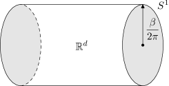
Figure 1: Spacetime geometry for the partition function in (3).

As a quantum statistical mechanical system, the partition function in the limit $L,\,A\to\infty$ is

$$Z=e^{-\beta V\,{\cal F}(\beta)}$$ (3)

where $V=L\cdot A$ and ${\cal F}$ is the free energy density. Standard results give:

$${\cal F}(\beta)=\dfrac{1}{\beta}\int\dfrac{d^{d}{\bf{k}}}{(2\pi)^{d}}\,\log\left(1-e^{-\beta k}\right).$$ (4)

The euclidean rotational symmetry allows one to view the above system with time now along the $\widehat{y}$ direction. In $1d$, interchanging the role of $\widehat{x}$ and $\widehat{y}$ is a special case of a modular transformation of the torus. In this version, the problem is a zero temperature quantum mechanical system with a finite size $\beta$ in one direction, and the total volume of the system is $V^{\prime}=\beta\cdot A$. The quantum mechanical path integral leads to

$$Z=e^{-LE_{0}(A,\beta)}$$ (5)

where $E_{0}$ is the ground state energy. Let ${\cal E}_{0}=E_{0}/V^{\prime}$ denote the ground state energy per volume. Comparing the two “channels”, their equivalence requires ${\cal E}_{0}(\beta)={\cal F}(\beta)$. In this finite-size channel, the modes of the field in the $\widehat{x}$ direction are quantized with wave-vector $k_{x}=2\pi n/\beta$, and the calculation of ${\cal E}_{0}$ is as in the Casimir effect (see below):

$${\cal E}_{0}=\dfrac{1}{2\beta}\sum_{n\in\mathbb{Z}}\int\dfrac{d^{d-1}{\bf{k}}}{(2\pi)^{d-1}}\left({\bf{k}}^{2}+\left(2\pi n/\beta\right)^{2}\right)^{1/2}.$$ (6)

The free energy density ${\cal F}$ can be calculated using

$$\int d^{d}{\bf{k}}=\dfrac{2\pi^{d/2}}{\Gamma(d/2)}\int d|{\bf{k}}|\,|{\bf{k}}|^{d-1}.$$ (7)

For $d>0$ the integral is convergent and one finds

$${\cal F}=-\dfrac{1}{\beta^{d+1}}\,\dfrac{\Gamma(d+1)\,\zeta(d+1)}{2^{d-1}\pi^{d/2}d\,\Gamma(d/2)}.$$ (8)

For the Casimir energy, after performing the ${\bf{k}}$ integral, ${\cal E}_{0}$ involves $\sum_{n\in\mathbb{Z}}|n|^{d}$ which must be regularized. As is usually done, let us regularize this as $2\,\zeta(-d)$. Then

$${\cal E}_{0}=-\dfrac{1}{\beta^{d+1}}~{}\pi^{d/2}\Gamma(-d/2)\zeta(-d).$$ (9)

Let us analytically continue in $d$ and define the function

$$\chi(z)\equiv\pi^{-z/2}\Gamma(z/2)\zeta(z).$$ (10)

Then the equality ${\cal E}_{0}={\cal F}$ requires the identity

$$\chi(z)=\chi(1-z).$$ (11)

The above relation is a known functional identity that was proven by Riemann using complex analysis. It will play an essential role in the rest of these lectures.

The above calculations show that $\zeta$-function regularization of the ground state energy ${\cal E}_{0}$ is consistent with a modular transformation to the finite-temperature channel. Our calculations can thus be viewed as a proof of the identity (11) based on physical consistency.

For spatial dimension $d=3$, the ground state energy ${\cal E}_{0}$ is closely related to the measurable Casimir effect, the difference only being in the boundary conditions. In the Casimir effect one measures the ground state energy of the electromagnetic field between two plates by measuring the force as one varies their separation, as illustrated in Figure 2.

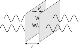
Figure 2: Geometry of the Casimir effect.

There is a simple relation between the vacuum energy densities $\rho$ in the cylindrical geometry above, and that of the usual Casimir effect:

$$\rho_{\rm vac}^{\rm casimir}(\ell)=2\rho_{\rm vac}^{\rm cylinder}(\beta=2\ell)=-\dfrac{\pi^{2}}{720\ell^{4}}.$$ (12)

It is remarkable that since the Casimir effect has been measured in the laboratory, such a measurement verifies

$$\zeta(-3)=1+2^{3}+3^{3}+4^{3}+\dotsm=\dfrac{1}{120}.$$ (13)

Of course the above equation is non-sense on its own. It only makes sense after analytically continuing $\zeta(z)$ from $\Re(z)>1$ to the rest of the complex plane.

II.2 Bose-Einstein condensation and the pole of $\zeta$

It is known that $\zeta(z)$ has only one pole, a simple one at $z=1$. This property is also related to some basic physics. In the phenomenon of Bose-Einstein condensation, below a critical temperature $T$ most of the bosonic particles occupy the lowest energy single particle state. This critical temperature depends on the density $n$. In $d$ spatial dimensions the formula reads

$$n=\int\dfrac{d^{d}{\bf{k}}}{(2\pi)^{d}}\dfrac{1}{e^{\omega_{\bf{k}}/T}-1}=\left(\dfrac{mT}{2\pi}\right)^{d/2}\zeta(d/2).$$ (14)

The Coleman-Mermin-Wagner theorem in statistical physics says that Bose-Einstein condensation is impossible in $d=2$ spatial dimensions. This is manifest in the above formula since $\zeta(1)=\infty$.

III Important properties of $\zeta$

After having discussed some applications of $\zeta$ in physics, let us now focus on its most basic mathematical properties as a complex analytic function.

III.1 Series representation

The $\zeta$-function is defined for $\Re(z)>1$ through the series

$$\zeta(z)=\sum_{n=1}^{\infty}\dfrac{1}{n^{z}}.$$ (15)

The first appearance of $\zeta(z)$ was in the so called “Basel problem” posed by Pietro Mengoli in $1644$. This problem consists in finding the precise sum of the infinite series of squares of natural numbers:

$$\zeta(2)=\sum_{n=1}^{\infty}\dfrac{1}{n^{2}}=\dfrac{1}{1^{2}}+\dfrac{1}{2^{2}}+\dfrac{1}{3^{2}}+\dotsb=\,?$$ (16)

The leading mathematicians of that time, like the Bernoulli family, attempted the problem unsuccessfully. It was only in $1735$ that Euler, with $28$ years old, solved the problem claiming that such sum is equal to $\pi^{2}/6$, and was brought to fame. Nevertheless, his arguments were not fully justified, as he manipulated infinite series with abandon, and only in $1741$ that Euler could built a formal proof. Even such a proof had to wait $100$ years until all the steps could be rigorously justified by the Weierstrass factorization theorem. Just as a curiosity let us reproduce Euler’s steps. From the Taylor series of $\sin z$ we have

$$\dfrac{\sin\pi z}{\pi z}=1-\dfrac{\left(\pi z\right)^{2}}{3!}+\dfrac{(\pi z)^{4}}{5!}+\dotsb.$$ (17)

From the Weierstrass product formula for the $\Gamma(z)$ function it is possible to obtain the product formula for $\sin z$ which reads

$$\dfrac{\sin\pi z}{\pi z}=\prod_{n=1}^{\infty}\left(1-\left(\dfrac{z}{n}\right)^{2}\right).$$ (18)

Now collecting terms of powers of $z$ in (18) one finds

$$\dfrac{\sin\pi z}{\pi z}=1-z^{2}\sum_{n=1}^{\infty}\dfrac{1}{n^{2}}+z^{4}\sum_{\begin{subarray}{c}n,m=1\\ m>n\end{subarray}}^{\infty}\dfrac{1}{n^{2}m^{2}}+\dotsb.$$ (19)

Comparing the $z^{2}$ coefficient of (19) and (17) we immediately obtain Euler’s result,

$$\zeta(2)=\sum_{n=1}^{\infty}\dfrac{1}{n^{2}}=\dfrac{\pi^{2}}{6}.$$ (20)

Comparing the $z^{4}$ coefficients we have

$$\sum_{\begin{subarray}{c}n,m=1\\ m>n\end{subarray}}^{\infty}\dfrac{1}{n^{2}m^{2}}=\dfrac{\pi^{4}}{5!}.$$ (21)

Now consider the full range sum

$$\sum_{n,m=1}^{\infty}\dfrac{1}{n^{2}m^{2}}=\sum_{n=1}^{\infty}\dfrac{1}{n^{4}}+\sum_{\begin{subarray}{c}n,m=1\\ m>n\end{subarray}}^{\infty}\dfrac{1}{n^{2}m^{2}}+\sum_{\begin{subarray}{c}n,m=1\\ m<n\end{subarray}}^{\infty}\dfrac{1}{n^{2}m^{2}}.$$ (22)

The LHS is nothing but $\zeta^{2}(2)$. The first term in the RHS is $\zeta(4)$ and the two other terms are both equal to (21). Therefore we have

$$\zeta(4)=\sum_{n=1}^{\infty}\dfrac{1}{n^{4}}=\dfrac{\pi^{4}}{90}.$$ (23)

Considering the other powers $z^{2n}$ we can obtain $\zeta(2n)$ for even integers. We will see later a better approach to compute these values through an interesting relation with the Bernoulli numbers.

III.2 Convergence

Let us now analyze the domain of convergence of the series (15). Absolute convergence implies convergence, therefore it is enough to consider

$$\sum_{n=1}^{\infty}\dfrac{1}{|n^{z}|}=\sum_{n=1}^{\infty}\dfrac{1}{n^{x}},$$ (24)

where $z=x+iy$. Let $x=1+\delta$ with $\delta>0$. By the integral test we have

$$\int_{1}^{\infty}\dfrac{1}{u^{1+\delta}}\,du=-\dfrac{1}{\delta u^{\delta}}\bigg{|}_{1}^{\infty}=\dfrac{1}{\delta}.$$ (25)

If $\delta>0$ the above integral is finite, therefore the series is absolutely convergent for $\Re(z)>1$ and $\zeta(z)$ is an analytic function on this region. Note that if $\delta=0$ the above integral diverges as $\log(\infty)$. If $\delta\leq-1$ the integral also diverges. Therefore, the series representation given by (15) is defined only for $\Re(z)>1$.

III.3 The golden key: Euler product formula

The importance of the $\zeta$-function in number theory is mainly because of its relation to prime numbers. The first one to realize this connection was again Euler. To see this, let us consider the following product

$$\prod_{i=1}^{\infty}\left(1-\dfrac{1}{p_{i}^{z}}\right)^{-1}$$ (26)

where $p_{i}$ denotes a prime number, i.e. $p_{1}=2$, $p_{2}=3$ and so on. We know that $\left(1-z\right)^{-1}=\sum_{n=0}^{\infty}z^{n}$ for $|z|<1$, thus (26) is equal to

$$\prod_{i=1}^{\infty}\sum_{n=0}^{\infty}\dfrac{1}{p_{i}^{nz}}=\left(1+\dfrac{1}{p_{1}^{z}}+\dfrac{1}{p_{1}^{2z}}+\dotsb\right)\times\left(1+\dfrac{1}{p_{2}^{z}}+\dfrac{1}{p_{2}^{2z}}+\dotsb\right)\times\dotsb.$$ (27)

If we open the product in (27) we have an infinite sum of terms, each one having the form

$$\left(p_{1}^{\alpha_{1}}p_{2}^{\alpha_{2}}\dotsc p_{j}^{\alpha_{j}}\right)^{-z}\quad\mbox{where}\ j=1,2,\dotsc\ \mbox{and}\ \alpha_{j}=0,1,2,\dotsc,$$ (28)

i.e. we have a finite product of primes raised to every possible power. From the fundamental theorem of arithmetic, also known as the unique prime factorization theorem, we know that every natural number can be expressed in exactly one way through a product of powers of primes; $n=p_{1}^{\alpha_{1}}p_{2}^{\alpha_{2}}\dotsc p_{j}^{\alpha_{j}}$ where $p_{1}<p_{2}<\dotsb<p_{j}$. Therefore (27) involves a sum of all natural numbers, which is exactly the definition (15). Thus we have the very important result known as the Euler product formula

$$\zeta(z)=\sum_{n=1}^{\infty}\dfrac{1}{n^{z}}=\prod_{i=1}^{\infty}\left(1-\dfrac{1}{p_{i}^{z}}\right)^{-1}.$$ (29)

This result is of course only valid for $\Re(z)>1$. A simpler derivation of it is also given in Section IV. From this formula we can easily see that there are no zeros in this region,

$$\zeta(z)\neq 0\qquad\mbox{for $\Re(z)>1$,}$$ (30)

since each factor $\left(1-p_{i}^{-z}\right)$ never diverges.

III.4 The Dirichlet $\eta$-function

Instead of the $\zeta$-function defined in (15), let us consider its alternating version

$$\eta(z)=\sum_{n=1}^{\infty}\dfrac{(-1)^{n-1}}{n^{z}}.$$ (31)

This series is known as the Dirichlet $\eta$-function. For an alternating series $\sum(-1)^{n-1}a_{n}$, if $\lim_{n\to\infty}a_{n}=0$ and $a_{n}>a_{n+1}$ then the series converges. We can see that both conditions are satisfied for (31) provided that $\Re(z)>0$.

The $\eta$-function (31) has a negative sign at even naturals:

$$\eta(z)=1-\dfrac{1}{2^{z}}+\dfrac{1}{3^{z}}-\dfrac{1}{4^{z}}+\dotsb.$$ (32)

On the other hand the $\zeta$-function (15) has only positive signs, thus if we multiply it by $2/2^{z}$ we double all the even naturals appearing in (32) but with a positive sign

$$\dfrac{2}{2^{z}}\zeta(z)=\dfrac{2}{2^{z}}+\dfrac{2}{4^{z}}+\dfrac{2}{6^{z}}+\dotsb.$$ (33)

Summing (32) and (33) we obtain $\zeta(z)$ again, therefore

$$\zeta(z)=\dfrac{1}{1-2^{1-z}}\,\eta(z).$$ (34)

In obtaining this equality we had to assume $\Re(z)>1$, nevertheless (31) is defined for $\Re(z)>0$, thus (34) yields the analytic continuation of $\zeta(z)$ in the region $\Re(z)>0$.

III.5 Analytic continuation

One of Riemann’s main contributions is the analytic continuation of the $\zeta$-function to the entire complex plane (except for a simple pole at $z=1$). Actually, Riemann was the first one to consider the function (15) over a complex field. Following his steps, let us start from the integral definition of the $\Gamma$-function

$$\Gamma(z)=\int_{0}^{\infty}u^{z-1}e^{-u}du.$$ (35)

Replacing $u\to nu$ and summing over $n$ we have

$$\Gamma(z)\sum_{n=1}^{\infty}\dfrac{1}{n^{z}}=\sum_{n=1}^{\infty}\int_{0}^{\infty}u^{z-1}e^{-nu}du.$$ (36)

If we are allowed to interchange the order of the sum with the integral, and noting that $\sum_{n=1}^{\infty}e^{-nz}=\left(e^{z}-1\right)^{-1}$, then formally we have

$$\Gamma(z)\zeta(z)=\int_{0}^{\infty}\dfrac{u^{z-1}}{e^{u}-1}du.$$ (37)

The integral in (36) converges for $\Re(z)>1$. Under this condition it is possible to show that the integral (37) also converges. Thus the step in going from (36) to (37) is justified as long as we assume $\Re(z)>1$.

Since the integrand in (37) diverges at $u=0$, let us promote $u$ to a complex variable and consider the following integral

$${\cal J}(z)=\dfrac{1}{2\pi i}\int_{{\cal C}}\dfrac{u^{z}}{e^{-u}-1}\dfrac{du}{u}$$ (38)

over the path ${\cal C}$ illustrated in Figure 3, which excludes the origin through a circle of radius $\delta<2\pi$, avoiding the pole of the integrand in (38).

Figure 3: Contour ${\cal C}={\cal C}_{1}+{\cal C}_{2}+{\cal C}_{3}$ excluding the origin. ${\cal C}_{2}$ has radius $\delta<2\pi$.

On ${\cal C}_{1}$ we choose $u=re^{-i\pi}$ then

$$\dfrac{1}{2\pi i}\int_{{\cal C}_{1}}\dfrac{u^{z}}{e^{-u}-1}\dfrac{du}{u}=-\dfrac{e^{-i\pi z}}{2\pi i}\int_{\delta}^{\infty}\dfrac{r^{z-1}}{e^{r}-1}dr.$$ (39)

Analogously, on ${\cal C}_{3}$ we choose $w=re^{i\pi}$, then we have

$$\lim_{\delta\to 0}\dfrac{1}{2\pi i}\left(\int_{{\cal C}_{1}}+\int_{{\cal C}_{3}}\right)\dfrac{u^{z}}{e^{-u}-1}\dfrac{du}{u}=\dfrac{\sin\pi z}{\pi}\int_{0}^{\infty}\dfrac{r^{z-1}}{e^{r}-1}dr.$$ (40)

For the integral over ${\cal C}_{2}$ we have $u=\delta e^{i\theta}$, and since we are interested in $\delta\to 0$ we obtain

$$\dfrac{1}{2\pi i}\int_{{\cal C}_{2}}\dfrac{u^{z}}{e^{-u}-1}\dfrac{du}{u}=\dfrac{\delta^{z}}{2\pi}\int_{-\pi}^{\pi}\dfrac{e^{i\theta z}}{e^{-\delta e^{i\theta}}-1}d\theta\approx-\dfrac{\delta^{z-1}}{2\pi}\int_{-\pi}^{\pi}e^{i\theta(z-1)}d\theta.$$ (41)

Thus we have

$$\left|\dfrac{1}{2\pi i}\int_{{\cal C}_{2}}\dfrac{u^{z}}{e^{-u}-1}\dfrac{du}{u}\right|\leq\dfrac{\delta^{x-1}}{2\pi}\int_{-\pi}^{\pi}e^{-y\theta}d\theta=\delta^{x-1}\dfrac{\sinh\pi y}{\pi y}.$$ (42)

Since we are assuming $x>1$, the above result vanishes when $\delta\to 0$. Therefore from (37) and (40) we conclude that

$$\zeta(z)=\dfrac{\pi\,{\cal J}(z)}{\Gamma(z)\sin\left(\pi z\right)}.$$ (43)

Using the well known identity

$$\Gamma(z)\Gamma(1-z)=\dfrac{\pi}{\sin\left(\pi z\right)}$$ (44)

we can further simplify (43) obtaining

$$\zeta(z)=\Gamma(1-z)\,{\cal J}(z).$$ (45)

Although in obtaining (45) we assumed $\Re(z)>1$, the function $\Gamma(z)$ and the integral (38) remains valid for every complex $z$. Thus we can define $\zeta(z)$ through (45) on the whole complex plane (except at $z=1$ as will be shown below). Since (45) and (15) are the same on the half plane $\Re(z)>1$, then (45) yields the analytic continuation of the $\zeta$-function to the entire complex plane. The function defined by (45) is known as the Riemann $\zeta$-function.

The integral (38) is an entire function of $z$, and $\Gamma(1-z)$ has simple poles at $z=1,2,\dots$. Since $\zeta(z)$ does not have zeros for $\Re(z)>1$ then ${\cal J}(z)$ must vanish at $z=2,3,\dots$. In fact it is easy to see this explicitly. Note that for $z=n\in\mathbb{Z}$ the integral (38) over ${\cal C}_{1}$ and ${\cal C}_{3}$ cancel each other, thus it remains the integral over ${\cal C}_{2}$ only. From Cauchy’s integral formula we have

$${\cal J}(n)=\lim_{u\to 0}\dfrac{u^{n}}{e^{-u}-1}=0\qquad(n=2,3,\dotsc).$$ (46)

Moreover, since ${\cal J}(n)=0$ for $n\geq 2$, cancelling the poles of $\Gamma(1-n)$, the only possible pole of $\zeta(z)$ occurs at $z=1$. From (46) we have ${\cal J}(1)=-1$, showing that $\zeta(z)$ indeed has a simple pole inherited from the simple pole of $\Gamma(0)$. Since this pole is simple, we can compute the residue of $\zeta(1)$ through

$$\mbox{Res}\,\zeta(1)=\lim_{z\to 1}\left(z-1\right)\zeta(z)=\lim_{z\to 1}\left(z-1\right)\Gamma(1-z){\cal J}(z)=-\Gamma(1){\cal J}(1)=1,$$ (47)

where we have used (45) and the well known property $\Gamma(z+1)=z\,\Gamma(z)$.

III.6 Functional equation

The functional equation was already motivated by physical arguments in (11). Now we proceed to derive it mathematically. There are at least $7$ different ways to do this Titchmarsh . We are going to present only one way, which we think is the simplest.

Let us now consider the following integral

$${\cal J}_{N}(z)=\dfrac{1}{2\pi i}\oint_{{\cal C}_{N}}\dfrac{u^{z-1}}{e^{-u}-1}du$$ (48)

with the path of integration ${\cal C}_{N}$ as shown in Figure 4. Note that the integrand has the poles $u_{n}=2\pi ni$ ($n\in\mathbb{Z}$) along the imaginary axis. On this contour $r<2\pi$ and $2\pi Ni<R<(2N+2)\pi i$, thus the annular region encloses $2N$ poles corresponding to $n=\pm 1,\pm 2,\dotsc,\pm N$.

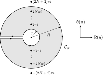
Figure 4: Contour ${\cal C}_{N}$ where $r<2\pi$ and $2N\pi<R<(2N+2)\pi$. This contour encloses $2N$ poles.

Let us first consider the integral (48) over the outer circle with radius $R$, i.e. $u=Re^{i\theta}$. Let $g(u)=\left(e^{-u}-1\right)^{-1}$. The function $g(u)$ is meromorphic, i.e. has only isolated singularities at $u_{n}=2\pi ni$. Around the circle of radius $R$ there are no singularities thus $g(u)$ is bounded in this region, i.e. $|g(u)|\leq M$. We also have $\left|u^{z-1}\right|=R^{x-1}e^{-\theta y}\leq R^{x-1}e^{|y|\pi}$. Therefore

$$\left|\int_{R}\dfrac{u^{z-1}}{e^{-u}-1}du\right|\leq\int_{-\pi}^{\pi}MR^{x-1}e^{|y|\pi}Rd\theta=2\pi MR^{x}e^{|y|\pi}.$$ (49)

Now if $N\to\infty$ then $R\to\infty$ and the above result goes to zero if $x<0$. In this way the only contribution from the integral (48) is due to the smaller circle $r$ and this is equal to the integral (38). Thus we conclude that

$$\lim_{N\to\infty}{\cal J}_{N}(z)={\cal J}(z)\qquad(\Re(z)<0).$$ (50)

We can now evaluate the integral (48) through the residue theorem. The integrand is $f(u)=u^{z-1}/\left(e^{-u}-1\right)$, then we have

$${\cal J}_{N}(z)=-\sum_{n=1}^{N+1}\left(\mbox{Res}f\left(u_{n}\right)+\mbox{Res}f\left(u_{-n}\right)\right),$$ (51)

where the minus sign is because the contour is traversed in the clockwise direction. The residue can be computed as follows:

$$\mbox{Res}f\left(u_{n}\right)=\lim_{u\to u_{n}}\left(u-u_{n}\right)f\left(u\right)=u_{n}^{z-1}\lim_{u\to u_{n}}\dfrac{u-u_{n}}{e^{-u}-1}=-(2\pi ni)^{z-1}.$$ (52)

Therefore,

$${\cal J}_{N}(z)=\sum_{n=1}^{N+1}(2\pi n)^{z-1}\left(i^{z-1}+(-i)^{z-1}\right)=2(2\pi)^{z-1}\cos\left(\pi(z-1)/2\right)\sum_{n=1}^{N+1}n^{z-1}.$$ (53)

Now the sum in (53) becomes particularly interesting if we replace $z\to 1-z$, yielding the same term $n^{-z}$ that appears in the series of the $\zeta$-function. In view of (50), now valid for $\Re(z)>1$, we thus have

$$\lim_{N\to\infty}{\cal J}_{N}(1-z)={\cal J}(1-z)=2(2\pi)^{-z}\cos\left(\pi z/2\right)\zeta(z).$$ (54)

Using (45) we obtain

$$\zeta(1-z)=2(2\pi)^{-z}\cos\left(\pi z/2\right)\Gamma(z)\zeta(z),$$ (55)

which relates $\zeta(z)$ to $\zeta(1-z)$. This equality can be written in a much more symmetric form using the following two well known properties of the $\Gamma$-function:

$$\Gamma(z)\Gamma(1-z) =\dfrac{\pi}{\sin(\pi z)},$$ (56)

$$\Gamma(z)\Gamma(z+1/2) =2^{1-2z}\sqrt{\pi}\,\Gamma(2z).$$ (57)

Replacing $z\to(z+1)/2$ in (56) and substituting into (55) we have

$$\zeta(1-z)=\dfrac{2(2\pi)^{-z}\pi\,\Gamma(z)\,\zeta(z)}{\Gamma\left((z+1)/2\right)\Gamma\left((1-z)/2\right)}.$$ (58)

Now replacing $z\to z/2$ in (57) and substituting the term $\Gamma(z)/\Gamma\left((z+1)/2\right)$ into the above equation we obtain

$$\chi(z)=\chi(1-z),\qquad\chi(z)\equiv\pi^{-z/2}\,\Gamma\left(z/2\right)\zeta(z).$$ (59)

This equality is known as the functional equation for the $\zeta$-function. This is an amazing relation, first discovered by Riemann. In deriving (59) we had to assume $\Re(z)>1$, but through analytic continuation it is valid on the whole complex plane, except at $z=1$ where $\zeta(z)$ has a simple pole. Note also that replacing $z\to 1+2n$ for $n=1,2,\dotsc$ into (55) we see that $\zeta(-2n)=0$, corresponding to the zeros of $\cos\left(\pi/2+n\pi\right)$.

III.7 Trivial zeros and specific values

We already have seen that due to the Euler product formula (29) $\zeta(z)$ have no zeros for $\Re(z)>1$. We have also seen in connection with (45) that $\zeta(z)$ has a simple pole at $z=1$. It follows from this pole that there are an infinite number of prime numbers. Moreover, due to (55) we have $\zeta(-2n)=0$ for $n=1,2,\dotsc$. These are the so called trivial zeros. Since there are no zeros for $\Re(z)>1$, the functional equation (59) implies that there are no other zeros for $\Re(z)<0$.

The other possible zeros of $\zeta(z)$ must therefore be inside the so-called critical strip, $0\leq\Re(z)\leq 0$. These are called the non-trivial zeros, since they can be complex contrary to the trivial ones. Note that from (59), since $\Gamma(z/2)$ has no zeros on the critical strip, then $\zeta(z)$ and $\chi(z)$ have the same zeros on this region. Moreover, these zeros are symmetric between the line $\Re(z)=1/2$. Since $\left(\chi(z)\right)^{*}=\chi(z^{*})$ if $\rho$ is a zero so is its complex conjugate $\rho^{*}$. Thus zeros occur in a quadruple: $\rho$, $\rho^{*}$, $1-\rho$ and $1-\rho^{*}$. The exception are for zeros on the so called critical line $\Re(z)=1/2$, where $\rho$ and $1-\rho^{*}$ coincide. It is known that there are an infinite number of zeros on the critical line. It remains unknown whether they are all simple zeros. We will discuss these non-trivial zeros in more detail later.

Now let us consider special values of the $\zeta$-function. Let us start by considering the negative integers $\zeta(-n)$. From (45) we have $\zeta(-n)=n!\,{\cal J}(-n)$. The integral (38) at this point can be computed through the residue theorem. Since the only pole is at $z=0$ we have

$$\zeta(-n)=n!\,\mbox{Res}\left.\left(\dfrac{u^{-n-1}}{e^{-u}-1}\right)\right|_{u=0}.$$ (60)

The Bernoulli polynomials $B_{n}(x)$ are defined through the generating function

$$\dfrac{ue^{xu}}{e^{u}-1}=\sum_{n=0}^{\infty}\dfrac{B_{n}(x)}{n!}u^{n}\qquad(|u|<2\pi).$$ (61)

The values $B_{n}\equiv B_{n}(0)$ are called Bernoulli numbers and defined by setting $x=0$ in (61). Then using (61) into (60) we have

$$\zeta(-n)=n!\,\mbox{Res}\left.\left(-u^{-n-2}\sum_{m=0}^{\infty}\dfrac{B_{m}(1)}{m!}u^{m}\right)\right|_{u=0}=-\dfrac{B_{n+1}(1)}{n+1}.$$ (62)

From the well known relation $B_{n}(x+1)-B_{n}(x)=nx^{n-1}$ for $n\geq 1$ we have $B_{n}(1)=B_{n}(0)$ for $n\geq 2$. Thus we have

$$\zeta(-n)=-\dfrac{B_{n+1}}{n+1}\qquad(n\geq 1).$$ (63)

The case $\zeta(0)$ can be obtained from (62) since $B_{1}(1)=1/2$, then $\zeta(0)=-1/2$. Also, since $B_{2n+1}=0$ we see once again that $\zeta(-2n)=0$ for $n\geq 1$.

Setting $z=2k$ in (55) we have $\zeta(1-2k)=2(2\pi)^{-2k}\cos\left(\pi k\right)\Gamma(2k)\zeta(2k)$, but from (63) we have $\zeta(1-2k)=-B_{2k}/2k$, and thus we have $\zeta(z)$ over the positive even integers,

$$\zeta(2k)=(-1)^{k+1}\dfrac{(2\pi)^{2k}B_{2k}}{2(2k)!}\qquad(k\geq 1).$$ (64)

The previous results (20) and (23) are particular cases of the above formula.

A very interesting question concerns the values of $\zeta(2k+1)$. Setting $z=2k+1$ into (55) we get zero on both sides, and for $z=-2k$ the poles of $\Gamma(-2k)$ cancel with the zeros of $\zeta(-2k)$ but this product is still undetermined, so we get no information about $\zeta(2k+1)$. No simple formula analogous to (64) is known for these values. It is known that $\zeta(3)$ is irrational, this number is called Apéry’s constant Apery1 ; Apery2 ; Beukers ; Zudilin . It is also known that there are infinite numbers in the form $\zeta(2k+1)$ which are irrational Rivoal . Due to the unexpected nature of the result, when Apéry first showed his proof many mathematicians considered it as flawed, however, H. Cohen, H. Lenstra and A. van der Poorten confirmed that in fact Apéry was correct. It has been conjectured that $\zeta(2k+1)/\pi^{2k+1}$ is transcendental Kohnen . A very interesting physical connection, providing a link between number theory and statistical mechanics, is that the most fundamental correlation function of the $XXX$ spin-$1/2$ chain can be expressed in terms of $\zeta(2k+1)$ Korepin .

IV Gauss and the prime number theorem

Let $\pi(x)$ denote the number of primes less than the positive real number $x$. It is a staircase function that jumps by one at each prime. In 1792, Gauss, when only 15 years, based on examining data on the known primes, guessed that their density went as $1/\log(x)$. This leads to the approximation

$$\pi(x)=\sum_{p\leq x}1\approx{\rm Li}(x)$$ (65)

where ${\rm Li}(x)$ is the log-integral function,

$${\rm Li}(x)=\int_{0}^{x}\dfrac{dt}{\log t}.$$ (66)

${\rm Li}(x)$ is a smooth function, and does indeed provide a smooth approximation to $\pi(x)$ as Figure 5 shows.

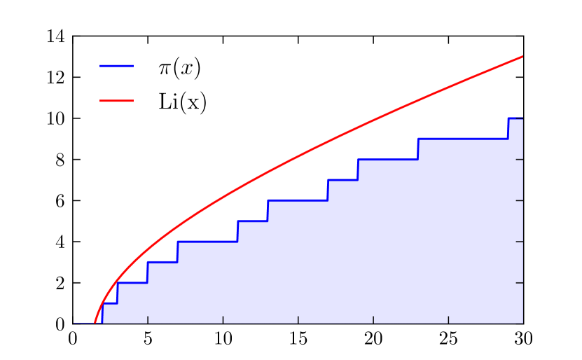
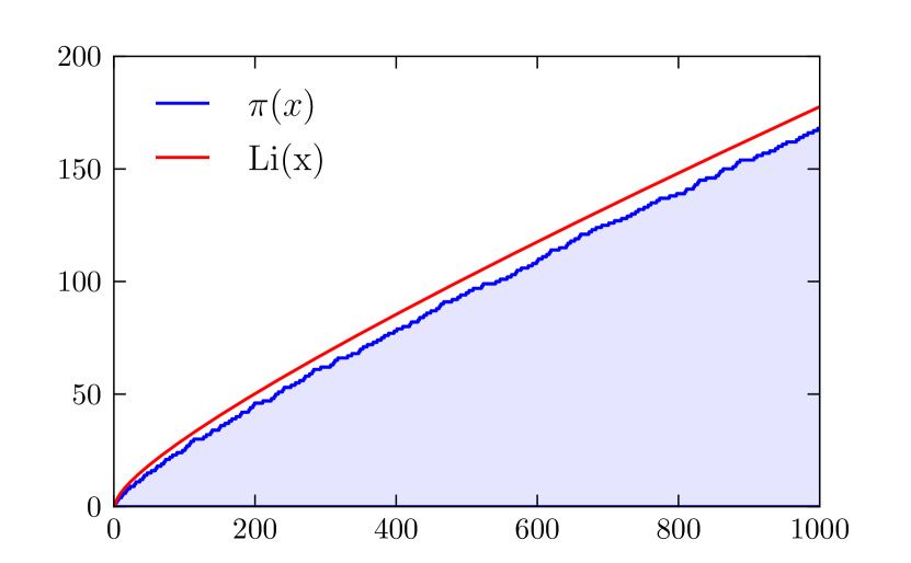
Figure 5: The ${\rm Li}(x)$ approximation to the prime number counting function $\pi(x)$.

The Prime number theorem (PNT) is the statement that ${\rm Li}(x)$ is the leading approximation to $\pi(x)$. It was only proven 100 years later using the main result of Riemann described in the next section. As we will explain later, the PNT follows if there are no Riemann zeros with $\Re(z)=1$.

The key ingredient in Riemann’s derivation of his result is the Euler product formula relating $\zeta(z)$ to the prime numbers. A simple derivation of Euler’s formula is based to the ancient “sieve” method for locating primes. One begins with a list of integers. First one removes all even integers, then all multiples of $3$, then all multiples of $5$, and so on. Eventually one ends up with the primes. We can describe this procedure analytically as follows. Begin with

$$\zeta(z)=1+\dfrac{1}{2^{z}}+\dfrac{1}{3^{z}}+\dfrac{1}{4^{z}}+\dotsm.$$ (67)

One has

$$\dfrac{1}{2^{z}}\zeta(z)=\dfrac{1}{2^{z}}+\dfrac{1}{4^{z}}+\dfrac{1}{6^{z}}+\dotsm$$ (68)

thus

$$\left(1-\dfrac{1}{2^{z}}\right)\zeta(z)=1+\dfrac{1}{3^{z}}+\dfrac{1}{5^{z}}+\dotsm.$$ (69)

Repeating this process with powers of $3$ we have

$$\left(1-\dfrac{1}{3^{z}}\right)\left(1-\dfrac{1}{2^{z}}\right)\zeta(z)=1+\dfrac{1}{5^{z}}+\dfrac{1}{7^{z}}+\dotsm.$$ (70)

Continuing this process to infinity, the right hand side equals $1$. Thus

$$\zeta(z)=\prod_{p}\dfrac{1}{1-p^{-z}}.$$ (71)

Chebyshev tried to prove the PNT using $\zeta(z)$ in 1850. It was finally proven in 1896 by Hadamard and de la Vallé Poussin by demonstrating that $\zeta(z)$ indeed has no zeros with $\Re(z)=1$.

V Riemann zeros and the primes

V.1 Riemann’s main result

Riemann obtained an explicit and exact expression for $\pi(x)$ in terms of the non-trivial zeros $\rho$ of $\zeta(z)$. There are simpler but equivalent versions of the main result, based on the function $\psi(x)$ below. However, let us present the main formula for $\pi(x)$ itself, since it is historically more important. The derivation is given in the next subsection.

The function $\pi(x)$ is related to another number-theoretic function $J(x)$, defined as

$$J(x)=\sum_{2\leq n\leq x}\dfrac{\Lambda(n)}{\log n}$$ (72)

where $\Lambda(n)$, the von Mangoldt function, is defined by

$$\Lambda(n)=\begin{cases}\log p&\mbox{if $n=p^{m}$ for some prime $p$ and integer $m\geq 1$,}\\ 0&\mbox{otherwise.}\end{cases}$$ (73)

For instance $\Lambda(3)=\Lambda(9)=\log 3$. The two functions $\pi(x)$ and $J(x)$ are related by Möbius inversion as follows:

$$\pi(x)=\sum_{n\geq 1}\dfrac{\mu(n)}{n}J(x^{1/n}).$$ (74)

Here $\mu(n)$ is the Möbius function defined as follows. For $n>1$, through the prime decomposition theorem we can write $n=p_{1}^{\alpha_{1}}\dotsm p_{k}^{\alpha_{k}}$. Then

$$\mu(n)=\begin{cases}(-1)^{k}&\mbox{if $\alpha_{1}=\alpha_{2}=\dotsm=\alpha_{k}=1$,}\\ 0&\mbox{otherwise.}\end{cases}$$ (75)

We also have $\mu(1)=1$. Note that $\mu(n)=0$ if and only if $n$ has a square factor $>1$. The above expression (74) is actually a finite sum, since for large enough $n$, $x^{1/n}<2$ and $J=0$.

The main result of Riemann is a formula for $J(x)$, expressed as an infinite sum over non-trivial zeros $\rho$,

$$J(x)={\rm Li}(x)-\sum_{\rho}{\rm Li}\left(x^{\rho}\right)+\int_{x}^{\infty}\dfrac{dt}{\log t}~{}\dfrac{1}{\left(t^{2}-1\right)t}-\log 2.$$ (76)

Riemann derived the result (76) starting from the Euler product formula and utilizing some insightful complex analysis that was sophisticated for the time. Some care must be taken in numerically evaluating ${\rm Li}(x^{\rho})$ since it has a branch point. It is more properly defined through the exponential integral function

$${\rm Li}(x)={\rm Ei}(\rho\log x),\qquad{\rm Ei}(z)=-\int_{-z}^{\infty}dt\,\dfrac{e^{-t}}{t}.$$ (77)

The sum in (76) is real because the $\rho$’s come in conjugate pairs. If there are no zeros on the line $\Re(z)=1$, then the dominant term is the first one, i.e. $J(x)\sim{\rm Li}(x)$, and this proves the PNT. The sum over $\rho$ corrections to ${\rm Li}(x)$ deform it to the staircase function $\pi(x)$ as Figure 6 shows. Thus, the complete knowledge of the primes is contained in the Riemann zeros.

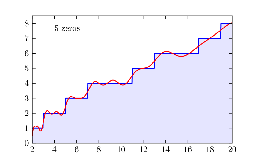
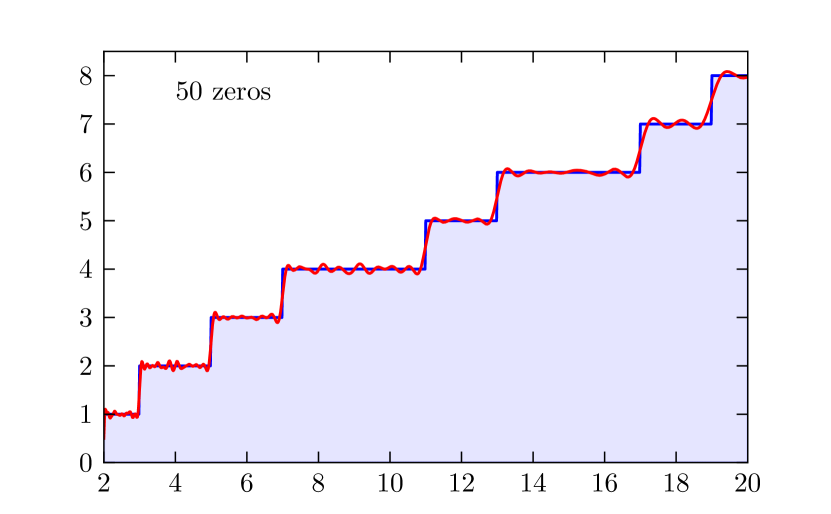
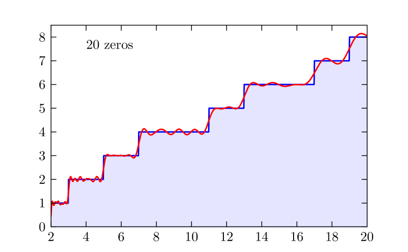
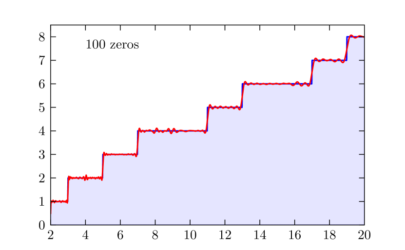
Figure 6: The function $\pi(x)$ as a sum of Riemann zeros from equations (74) and (76). The dashed (blue) region represents the exact $\pi(x)$ while the (red) oscillating curve is (74), obtained with different number of zeros as indicated in the figures.

Von Mangoldt provided a simpler formulation based on the function

$$\psi(x)=\sum_{n\leq x}\Lambda(n).$$ (78)

The function $\psi(x)$ has a simpler expression in terms of Riemann zeros which reads

$$\psi(x)=x-\sum_{\rho}\dfrac{x^{\rho}}{\rho}-\log(2\pi)-\dfrac{1}{2}\log\left(1-\dfrac{1}{x^{2}}\right).$$ (79)

In this formulation, the PNT follows from the fact that the leading term is $\psi(x)\sim x$.

V.2 $\psi(x)$ and the Riemann zeros

We first derive the formula (79). From the Euler product formula one has

$$\partial_{z}\log\zeta(z)=-\sum_{p}\partial_{z}\log\left(1-p^{-z}\right)=-\sum_{p}\log p\,\dfrac{p^{-z}}{1-p^{-z}}.$$ (80)

Taylor expanding the factor $1/(1-p^{-z})$ one obtains

$$\partial_{z}\log\zeta(z)=-\sum_{p}\sum_{m=1}^{\infty}\dfrac{\log p}{p^{mz}}.$$ (81)

For any arithmetic function $a(n)$, the Perron formula relates

$$A(x)=\sum_{n\leq x}{}^{{}^{\prime}}a(n)$$ (82)

to the poles of the Dirichlet series

$$g(z)=\sum_{n=1}^{\infty}\dfrac{a(n)}{n^{z}}.$$ (83)

In (82) the restriction on the sum is such that if $x$ is an integer, then the last term of the sum must be multiplied by $1/2$. Now $\zeta(z)$ can be factored in terms of its zeros, $\zeta(z)\propto\prod_{\rho}(z-\rho)$, thus $\partial_{z}\log\zeta(z)$ has poles at each zero $\rho$. This implies that the Perron formula can be used to relate $\psi(x)$ to the Riemann zeros.

The Perron formula is essentially an inverse Mellin transform. If the series for $g(z)$ converges for $\Re(z)>z_{1}$, then

$$A(x)=\dfrac{1}{2\pi i}\int_{c-i\infty}^{c+i\infty}\dfrac{dz}{z}\,g(z)\,x^{z}$$ (84)

where the $z$-contour of integration is a straight vertical line from $-\infty$ to $+\infty$ with $c>z_{1}$. For completeness, we present a derivation of this formula in Appendix A.

Let us apply the Perron formula to $\psi(x)$,

$$\psi(x)=\dfrac{1}{2\pi i}\int_{c-i\infty}^{c+i\infty}\dfrac{dz}{z}~{}g(z)\,x^{z}$$ (85)

where $g(z)=-\partial_{z}\log\zeta(z)$ and $c>1$. The line of integration can be made into a closed contour by closing at infinity with $\Re(z)\leq c$. Now

$$g(z)=-\partial_{z}\left(\sum_{\rho}\log(z-\rho)+\sum_{\rho^{\prime}}\log(z-\rho^{\prime})-\log(z-1)\right)$$ (86)

where $\rho$ are zeros of $\zeta(z)$ on the critical strip and $\rho^{\prime}$ are the trivial zeros on the negative real axis at $\rho^{\prime}=-2n$. The $-\log(z-1)$ is due to the pole at $z=1$. The sum of the residues gives

$$\psi(x)=x-\sum_{\rho}\dfrac{x^{\rho}}{\rho}-\sum_{\rho^{\prime}}\dfrac{x^{\rho^{\prime}}}{\rho^{\prime}}+g(0).$$ (87)

The first term comes from the $z=1$ pole and $g(0)=-\log(2\pi)$ comes from the $z=0$ pole. Finally

$$\sum_{\rho^{\prime}}\dfrac{x^{\rho^{\prime}}}{\rho^{\prime}}=-\sum_{n=1}^{\infty}\dfrac{x^{-2n}}{2n}=\dfrac{1}{2}\log(1-1/x^{2})$$ (88)

and this gives the result (79).

V.3 $\pi(x)$ and the Riemann zeros

Let us first explain the relation (74) between $\pi(x)$ and $J(x)$ involving the Möbius $\mu$ function. By definition, $J(x)=0$ for $x<2$. It jumps by $1/n$ at each $x=p^{n}$ where $p$ is a prime. The expression (74) is always a finite sum since for $n$ large enough $x^{1/n}<2$. Consider for instance the range $x\leq 10$. $J(x)$ in this range is plotted in Figure 7.

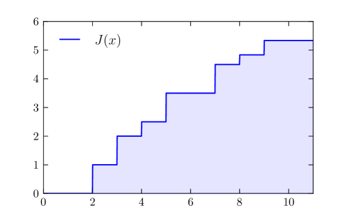
Figure 7: The number theoretic function $J(x)$ for $x<11$.

Since $10^{1/4}<2$, the formula (74) gives

$$\pi(x)=J(x)-\dfrac{1}{2}J(x^{1/2})-\dfrac{1}{3}J(x^{1/3}).$$ (89)

One easily sees that the two subtractions remove from $J(x)$ the jumps by $1/2$ at $x=2^{2},3^{2}$ and the jump by $1/3$ at $x=2^{3}$ leaving only the jumps by one at the primes $2,3,5,7$.

Let us now derive (76). Comparing definitions, one has

$$dJ(x)=\dfrac{1}{\log x}d\psi(x).$$ (90)

Integrating this

$$J(x)=\int_{0}^{x}\dfrac{dt}{\log t}\dfrac{d\psi(t)}{dt}=\int_{0}^{x}\dfrac{dt}{\log t}\left(1-\sum_{\rho}t^{\rho-1}-\dfrac{1}{t(t^{2}-1)}\right).$$ (91)

Making the change of variables $y=t^{\rho}$,

$$\int_{0}^{x}\dfrac{dt}{\log t}t^{\rho-1}=\int_{0}^{x^{\rho}}\dfrac{dy}{\log y}={\rm Li}(x^{\rho}).$$ (92)

Finally using

$$\int_{0}^{x}\dfrac{dt}{\log t}\dfrac{1}{(t^{2}-1)t}+\int_{x}^{\infty}\dfrac{dt}{\log t}\dfrac{1}{(t^{2}-1)t}=\log 2$$ (93)

one obtains the form (76).

VI An electrostatic analogy

A complex function is difficult to visualize since it is a hypersurface in a $4$ dimensional space. In this section we construct an electric field and electric potential and use them to visualize the RH through a single real scalar field over the $2$ dimensional $(x,y)$-plane, where $z=x+iy$.

VI.1 The electric field

Let us remove the $z=1$ pole in $\chi(z)$ while maintaining its symmetry under $z\to 1-z$ by defining the function

$$\xi(z)\equiv\tfrac{1}{2}z(z-1)\chi(z)=\tfrac{1}{2}z(z-1)\pi^{-z/2}\Gamma(z/2)\zeta(z)$$ (94)

which satisfies

$$\xi(z)=\xi(1-z).$$ (95)

Let us define the real and imaginary parts of $\xi(z)$ as

$$\xi(z)=u(x,y)+i\,v(x,y)$$ (96)

The Cauchy-Riemann equations

$$\partial_{x}u=\partial_{y}v,\qquad\partial_{y}u=-\partial_{x}v$$ (97)

are satisfied everywhere since $\xi$ is an entire function. Consequently, both $u$ and $v$ are harmonic functions, i.e. solutions of the Laplace equation $\vec{\nabla}^{2}u=(\partial_{x}^{2}+\partial_{y}^{2})u=0$ and $\vec{\nabla}^{2}v=0$, although they are not completely independent. Let us define $u$ or $v$ contours as the curves in the $x$-$y$ plane corresponding to $u$ or $v$ equal to a constant, respectively. The critical line is a $v=0$ contour since $\xi$ is real along it. As a consequence of the Cauchy-Riemann equations we have

$$\vec{\nabla}u\cdot\vec{\nabla}v=0.$$ (98)

Thus where the $u$ and $v$ contours intersect, they are necessarily perpendicular, and this is one aspect of their dependency. A Riemann zero occurs wherever the $u=0$ and $v=0$ contours intersect, as illustrated in Figure 8.

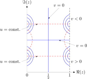
Figure 8: $u$ contours are dashed (red) lines and $v$ contours are solid (blue) lines. A Riemann zero on occurs where a $u=0$ contour spans the entires strip and passes through the zero on the critical line which is a $v=0$ contour.

From the symmetry (95) and $\xi(z)^{*}=\xi(z^{*})$ it follows that

$$u(x,y)=u(1-x,y),\qquad v(x,y)=-v(1-x,y).$$ (99)

This implies that the $v$ contours do not cross the critical line except for $v=0$. All the $u$ contours on the other hand are allowed to cross it by the above symmetry. Away from the $v=0$ points on the line $\Re(z)=1$, since the $u$ and $v$ contours are perpendicular, the $u$ contours generally cross the critical line and span the whole strip due to the symmetry (99). The $u$ contours that do not cross the critical line must be in the vicinity of the $v=0$ contours, again by the perpendicularity of their intersections. Figure 8 depicts the behavior of the $u$ and $v$ contours in regions of the critical strip with no zeros off of the line.

Introduce the vector field

$$\vec{E}=E_{x}\,\widehat{x}+E_{y}\,\widehat{y}\equiv u(x,y)\,\widehat{x}-v(x,y)\,\widehat{y}$$ (100)

where $\widehat{x}$ and $\widehat{y}$ are unit vectors in the $x$ and $y$ directions. This field has zero divergence and curl as a consequence of the Cauchy-Riemann equations,

$$\vec{\nabla}\cdot\vec{E}=0,\qquad\vec{\nabla}\times\vec{E}=0,$$ (101)

which are defined everywhere since $\xi$ is entire. Thus it satisfies the conditions of a static electric field with no charged sources. We are only interested in the electric field on the critical strip. $\vec{E}$ is not a physically realized electric field here, in that we do not need to specify what kind of charge distribution would give rise to such a field. All of our subsequent arguments will be based only on the mathematical identities expressed in equation (101), and our reference to electrostatics is simply a useful analogy. Since the divergence of $\vec{E}$ equals zero everywhere, the hypothetical electric charge distribution that gives rise to $\vec{E}$ should be thought of as existing at infinity. Alternatively, since $u$ and $v$ are harmonic functions, one can view them as being determined by their values on the boundary of the critical strip.

As we now argue, the main properties of the above $\vec{E}$ field on the critical strip are determined by its behavior near the Riemann zeros on the critical line combined with the behavior near $\Re(z)=1$. In particular, electric field lines do not cross. Any Riemann zero on the critical line arises from a $u=0$ contour that crosses the full width of the strip and thus intersects the vertical $v=0$ contour. On the $u=0$ contour, $E_{x}=0$, whereas on the $v=0$ contour of the critical line itself, $E_{y}=0$. Furthermore, $E_{y}$ changes direction as one crosses the critical line. Finally, taking into account that $\vec{E}$ has zero curl, one can easily see that there are only two ways that all these conditions can be satisfied near the Riemann zero. One is shown in Figure 9 (left), the second has the direction of all arrows reversed. In short, Riemann zeros on the critical strip are manifestly consistent with the necessary properties of $\vec{E}$.

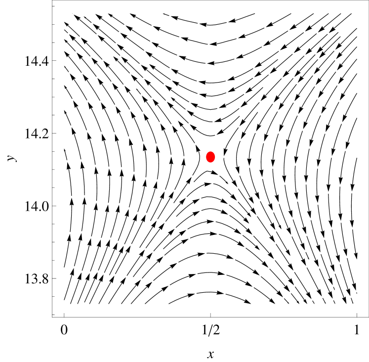
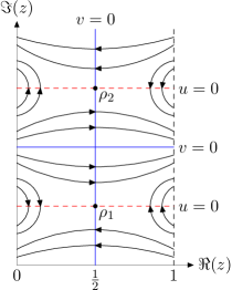
Figure 9: Left: field lines of $\vec{E}(x,y)$, equation (100), in the vicinity of the first Riemann zero. Right: illustration of the field $\vec{E}(x,y)$ in the vicinity of two consecutive Riemann zeros $\rho_{1}$ and $\rho_{2}$ on the critical line.

We now turn to the global properties of $\vec{E}$ along the entire critical strip. The electric field must alternate in sign from one zero to the next, otherwise the curl of $\vec{E}$ would not be zero in a region between two consecutive zeros. Thus there is a form of quasi-periodicity along the critical line, in the sense that zeros alternate between being even and odd, like the integers, and also analogous to the zeros of $\sin x$ at $x=\pi n$ where $e^{i\pi n}=(-1)^{n}$. Also, along the nearly horizontal $v=0$ contours that cross the critical line, $\vec{E}$ is in the $x$ direction. This leads to the pattern in Figure 9 (right). One aspect of the rendition of this pattern is that it implicitly assumes that the $v=0$ and $u=0$ points along the line $\Re(z)=1$ alternate, namely, between two consecutive $v=0$ points along this line, there is only one $u=0$ point, which is consistent with the knowledge that there are no zeros of $\xi$ along the line $\Re(z)=1$. This fact will be clearer when we reformulate our argument in terms of the potential $\Phi$ below.

VI.2 The electric potential $\Phi$

A mathematically integrated version of the above arguments, which has the advantage of making manifest the dependency of $u$ and $v$, can be formulated in terms of the electric potential $\Phi$ which is a single real function, defined to satisfy $\vec{E}=-\vec{\nabla}\Phi$. Although it contains the same information as the above argument, it is more economical.

By virtue of $\vec{\nabla}\cdot\vec{E}=0$, $\Phi$ is also a solution of Laplace’s equation $\partial_{z}\partial_{\overline{z}}\Phi=0$ where we denote ${\overline{z}}=z^{*}$. The general solution is that $\Phi$ is the sum of a function of $z$ and another function of ${\overline{z}}$. Since $\Phi$ must be real,

$$\vec{E}=-\vec{\nabla}\Phi,\qquad\Phi(x,y)=\tfrac{1}{2}\left(\varphi(z)+\overline{\varphi}({\overline{z}})\right)$$ (102)

where $\overline{\varphi}({\overline{z}})=\left(\varphi(z)\right)^{*}$. Clearly $\Phi$ is not analytic, whereas $\varphi$ is; it is useful to work with $\Phi$ since we only have to deal with one real function. Comparing the definitions of $\vec{E}$ and $\xi$ in terms of $u$ and $v$, one finds

$$u=-\tfrac{1}{2}\left(\partial_{z}\varphi+\partial_{\overline{z}}\overline{\varphi}\right),\qquad v=-\tfrac{i}{2}\left(\partial_{\overline{z}}\overline{\varphi}-\partial_{z}\varphi\right).$$ (103)

This implies

$$\xi(z)=-\dfrac{\partial\varphi(z)}{\partial z}$$ (104)

This equation can be integrated because $\xi$ is entire. Riemann’s original paper gave the following integral representation

$$\xi(z)=4\int_{1}^{\infty}dt\,G(t)\cosh\left[(z-\tfrac{1}{2})\log(t)/2\right]$$ (105)

where

$$G(t)=t^{-1/4}\partial_{t}\left(t^{3/2}\partial_{t}g\right),\qquad g(t)=\tfrac{1}{2}\left(\vartheta_{3}(0,e^{-\pi t})-1\right)=\sum_{n=1}^{\infty}e^{-n^{2}\pi t}.$$ (106)

Here, $\vartheta_{3}$ is one of the four elliptic theta functions. Note that the $z\to 1-z$ symmetry is manifest in this expression. Using this, then up to an irrelevant additive constant

$$\varphi(z)=-8\int_{1}^{\infty}\dfrac{dt}{\log t}\,G(t)\sinh\left[\tfrac{1}{2}(z-\tfrac{1}{2})\log t\right].$$ (107)

Let us now consider the $\Phi=\mbox{const.}$ contours in the critical strip. Using the integral representation (107), one finds the symmetry $\Phi(x,y)=-\Phi(1-x,y)$. One sees then that the $\Phi\neq 0$ contours do not cross the critical line, whereas the $\Phi=0$ contours can and do. Since $\varphi$ is imaginary along the critical line, the latter is also a $\Phi=0$ contour.

All Riemann zeros $\rho$ necessarily occur at isolated points, which is a property of entire functions. This is clear from the factorization formula $\xi(z)=\xi(0)\prod_{\rho}(1-z/\rho)$, conjectured by Riemann, and later proved by Hadamard. Where are these zeros located in terms of $\Phi$? At $\rho$, $\vec{\nabla}\Phi=0$. Thus, such isolated zeros occur when two $\Phi$ contours intersect, which can only occur if the two contours correspond to the same value of $\Phi$ since $\Phi$ is single-valued. A useful analogy is the electric potential for equal point charges. The electric field vanishes halfway between them, and this is the unique point where the equi-potential contours vanish. The argument is simple: $\vec{\nabla}\Phi$ is perpendicular to the $\Phi$ contours, however as one approaches $\rho$ along one contour, one sees that it is not in the same direction as inferred from the approach from the other contour. The only way this could be consistent is if $\vec{\nabla}\Phi=0$ at $\rho$. For purposes of illustration, we show the electric potential contours for two equal point charges in Figure 10 (left). Here, the electric field is only zero halfway between the charges, and indeed this is where two $\Phi$ contours intersect.

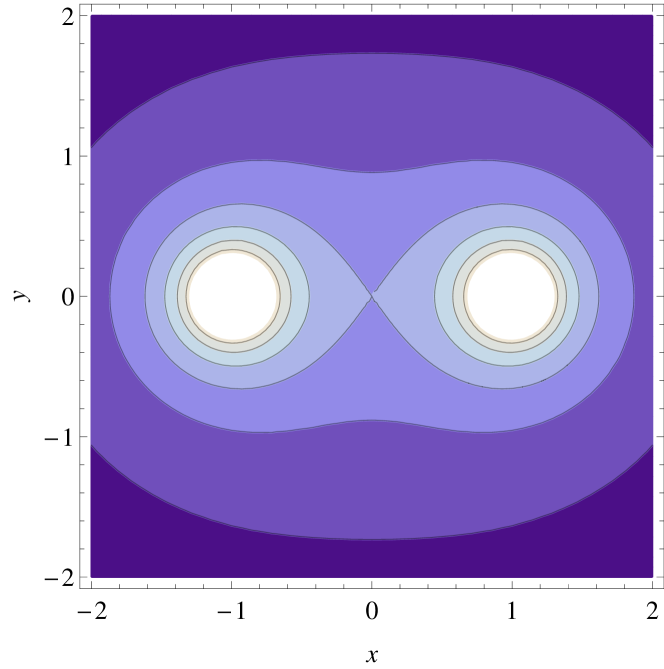
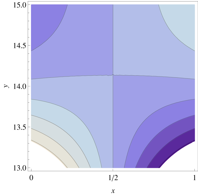
Figure 10: Left: the electric potential of two equal point charges. Right: contour plot of the potential $\Phi$ in the vicinity of the first Riemann zero at $\rho=\tfrac{1}{2}+(14.1347\dotsc)\,i$. The horizontal (vertical) direction is the $x$ ($y$) direction, where $z=x+iy$. The critical line and nearly horizontal line are $\Phi=0$ contours and they intersect at the zero.

With these properties of $\Phi$, we can now begin to understand the location of the known Riemann zeros. Since the $\Phi=0$ contours intersect the critical line, which itself is also a $\Phi=0$ contour, a zero exists at each such intersection, and we know there are an infinite number of them. The contour plot in Figure 10 (right) for the actual function $\Phi$ constructed above verify these statements. We emphasize that there is nothing special about the value $\Phi=0$, since $\Phi$ can be shifted by an arbitrary constant without changing $\vec{E}$; we defined it such that the critical line corresponds to $\Phi=0$.

A hypothetical Riemann zero off of the critical line would then necessarily correspond to an intersection of two $\Phi\neq 0$ contours. For simplicity, let us assume that only two such contours intersect, since our arguments can be easily extended to more of such intersections. Such a situation is depicted in Figure 11 (left).

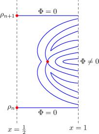
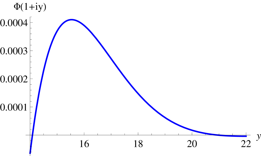
Figure 11: Left: a sketch of the contour plot of the potential $\Phi$ in the vicinity of a hypothetical Riemann zero off of the critical line. Such a zero occurs where the contours intersect. $\rho_{n}$ and $\rho_{n+1}$ are consecutive zeros on the line. Right: the electric potential between zeros on the boundary of the critical strip $\Re(z)=1$.

This figure implies that on the line $\Re(z)=1$, specifically $z=1+iy$, $\Phi$ takes on the same non-zero value at four different values of $y$ between consecutive zeros, i.e. roots of the equation $f(y)=0$, where

$$f(y)\equiv\Phi(1,y)=\Re(\varphi(1+iy)).$$ (108)

Thus, the real function $f(y)$ would have to have $3$ extrema between two consecutive zeros. Figure 11 (right) suggests that this does not occur. In order to attempt to prove it, let us define a “regular alternating” real function $h(y)$ of a real variable $y$ as a function that alternates between positive and negative values in the most regular manner possible: between two consecutive zeros $h(y)$ has only one maximum, or minimum. For example, the $\sin(y)$ function is obviously regular alternating. By the above argument, if $f(y)$ is regular alternating, then two $\Phi\neq 0$ contours cannot intersect and there are no Riemann zeros off the critical line. In Figure 11 (right) we plot $f(y)$ for low values of $y$ in the vicinity of the first two zeros, and as expected, it is regular alternating in this region.

To summarize, based on the symmetry (95), and the existence of the known infinity of Riemann zeros along the critical line, we have argued that $\vec{E}$ and $\Phi$ satisfy a regular repeating pattern all along the critical strip, and the RH would follow from such a repeating pattern. In order to go further, one obviously needs to investigate the detailed properties of the function $\xi$, in particular its large $y$ asymptotic behavior, and attempt to establish this repetitive behavior, more specifically, that $f(y)$ defined above is a regular alternating function.

VI.3 Analysis

In this subsection, we attempt to establish that $f(y)$ of the last section is a regular alternating function, however our results will not be conclusive. If $f(y)$ is a regular alternating function, then so is $\partial_{y}f(y)$:

$$\partial_{y}f(y)=\Im\left[\xi(1+iy)\right].$$ (109)

Thus, one only needs to show that $f^{\prime}(y)$ is regular alternating. Using the summation formula for $g(t)$, one can show

$$\begin{split}\xi(z)&=\lim_{N\to\infty}\xi^{(N)}(z)=\lim_{N\to\infty}\sum_{n=1}^{N}\xi_{n}(z),\\ \xi_{n}(z)&=n^{2}\pi\left[4e^{-\pi n^{2}}-z\,E_{\tfrac{z-1}{2}}(\pi n^{2})+(z-1)E_{-\tfrac{z}{2}}(\pi n^{2})\right].\end{split}$$ (110)

where $E_{\nu}(r)$ is an incomplete $\Gamma$ function

$$E_{\nu}(r)=\int_{1}^{\infty}dt\,e^{-rt}t^{-\nu}=r^{\nu-1}\,\Gamma(1-\nu,r).$$ (111)

It is sometimes referred to as the generalized exponential-integral function. In obtaining the above equation we have used the identity

$$rE_{\nu}(r)=e^{-r}-\nu E_{\nu+1}(r).$$ (112)

The nature of this approximation is that the roots $\rho$ of $\xi^{(N)}(\rho)=0$ provide a very good approximation to the smaller Riemann zeros for large enough $N$. However small values of $N$ are actually sufficient to a good degree of accuracy for small $y$. For instance, the first root for $\xi^{(3)}$ coincides with the first Riemann zero to 15 digits, and it’s sixth root is correct to 8 digits. Furthermore $\xi_{n+1}$ is smaller than $\xi_{n}$ because of the $e^{-n^{2}\pi t}$ suppression in the integrand for $E_{\nu}(\pi n^{2})$.

For $\nu$ large, one has the series

$$\begin{split}E_{\nu}(r)&=\sqrt{\dfrac{\pi}{2}}\,r^{\nu-1}\,\csc[(1-\nu)\pi]\,e^{-(\nu-1/2)\log\nu+\nu-1/12\nu+O(1/\nu^{3})}\\ &+\dfrac{e^{-r}}{\nu}\left\{1-\dfrac{(r-1)}{\nu}+\dfrac{(r^{2}-3r+1)}{\nu^{2}}+O\left((r/\nu)^{3}\right)\right\}.\end{split}$$ (113)

Using this, the leading term for large $y$ is

$$\Im\left[\xi_{n}(1+iy)\right]\approx-\dfrac{y^{2}\,e^{-\pi y/4}}{\sqrt{2}n}\sin\left[\dfrac{y}{2}\log\left(\dfrac{y}{2\pi n^{2}e}\right)\right].$$ (114)

To a reasonably good approximation, for large $y$, $\Im\left[\xi(1+iy)\right]\approx\Im\left[\xi_{1}(1+iy)\right]$, and (114) indeed is a regularly alternating function because the argument of the $\sin$ function is monotonic. However we cannot completely rule out that including the other terms in $\xi^{(N)}$ for $N>1$ could spoil this behavior.

VII Transcendental equations for zeros of the $\zeta$-function

The main new result presented in the next few sections are transcendental equations satisfied by individual zeros of some $L$-functions. For simplicity we first consider the Riemann $\zeta$-function, which is the simplest Dirichlet $L$-function. Moreover, we first consider the asymptotic equation (131), first proposed in RHLeclair , since it involves more familiar functions. This asymptotic equation follows trivially from the exact equation (138), presented later.

VII.1 Asymptotic equation satisfied by the $n$-th zero on the critical line

As above, let us define the function

$$\chi(z)\equiv\pi^{-z/2}\,\Gamma\left(z/2\right)\zeta(z).$$ (115)

which satisfies the functional equation

$$\chi\left(z\right)=\chi\left(1-z\right).$$ (116)

Now consider Stirling’s approximation

$$\Gamma(z)=\sqrt{2\pi}z^{z-1/2}e^{-z}\left(1+O\left(z^{-1}\right)\right)$$ (117)

where $z=x+iy$, which is valid for large $y$. Under this condition we also have

$$z^{z}=\exp\left(i\left(y\log y+\dfrac{\pi x}{2}\right)+x\log y-\dfrac{\pi y}{2}+x+O\left(y^{-1}\right)\right).$$ (118)

Therefore, using the polar representation

$$\zeta=|\zeta|e^{i\arg\zeta}$$ (119)

and the above expansions, we can write

$$\chi(z)=A\,e^{i\theta}$$

where

$$A(x,y) =\sqrt{2\pi}\,\pi^{-x/2}\left(\dfrac{y}{2}\right)^{(x-1)/2}e^{-\pi y/4}|\zeta(x+iy)|\left(1+O\left(z^{-1}\right)\right),$$ (120)

$$\theta(x,y) =\dfrac{y}{2}\log\left(\dfrac{y}{2\pi e}\right)+\dfrac{\pi}{4}(x-1)+\arg\zeta(x+iy)+O\left(y^{-1}\right).$$ (121)

The above approximation is very accurate. For $y$ as low as $100$, it evaluates $\chi\left(\tfrac{1}{2}+iy\right)$ correctly to one part in $10^{6}$. Above we are assuming $y>0$. The results for $y<0$ follows trivially from the relation $\left(\chi(z)\right)^{*}=\chi(z^{*})$.

We will need the result that the argument, $\arg f(z)$, of an analytic function $f(z)$ has a well defined limit at a zero $\rho$ where $f(\rho)=0$. Let ${\cal C}$ be a curve in the $z$-plane such that $z\left({\cal C}\right)$ approaches the zero $\rho$ in a smooth manner, namely, $z\left({\cal C}\right)$ has a well-defined tangent at $\rho$. Without loss of generality, let $\rho=0$. If the zero is of order $k$, then near zero

$$f(z)=a_{k}z^{k}+a_{k+1}z^{k+1}+\dotsm.$$ (122)

Then $\arg(f(z)/z^{k})$ converges to $\arg a_{k}$ along the curve ${\cal C}$. Since $z({\cal C})$ has a tangent at $0$, $\arg z({\cal C})$ converges to a limit $t$ as ${\cal C}$ approaches $\rho$, so that $\arg f(z)\to\arg(a_{k})+kt$ as ${\cal C}\to\rho$.

Now let $\rho=x+iy$ be a Riemann zero. Then $\arg\zeta(\rho)$ can be well-defined by the limit

$$\arg\zeta\left(\rho\right)\equiv\lim_{\delta\to 0^{+}}\arg\zeta\left(x+\delta+iy\right).$$ (123)

For reasons that are explained below, it is important that $0<\delta\ll 1$. This limit in general is not zero. For instance, for the first Riemann zero at $\rho=\tfrac{1}{2}+iy_{1}$, where $y_{1}=14.1347\dotsc$,

$$\arg\zeta\left(\tfrac{1}{2}+iy_{1}\right)\approx 0.157873919880941213041945.$$ (124)

On the critical line $z=\tfrac{1}{2}+iy$, if $y$ does not correspond to the imaginary part of a zero, the well-known function

$$S(y)=\dfrac{1}{\pi}\arg\zeta\left(\tfrac{1}{2}+iy\right)$$ (125)

is defined by continuous variation along the straight lines starting from $2$, then up to $2+iy$ and finally to $\tfrac{1}{2}+iy$, where $\arg\zeta(2)=0$ (see (293)). The function $S(y)$ is discussed in greater detail below in section VIII. On a zero, the standard way to define this term is through the limit $S(\rho)=\tfrac{1}{2}\lim_{\epsilon\to 0}\left(S\left(\rho+i\epsilon\right)+S\left(\rho-i\epsilon\right)\right)$. We have checked numerically that for several zeros on the line, our definition (123) gives the same answer as this standard approach. In any case our definition of $S(y)$ is perfectly valid in and of itself.

From (115) it follows that $\zeta(z)$ and $\chi(z)$ have the same zeros on the critical strip, so it is enough to consider the zeros of $\chi(z)$. Let us now consider approaching a zero $\rho=x+iy$ through the $\delta\to 0^{+}$ limit in $\arg\zeta$. Consider first the simple zeros along the critical line. Later we will argue that all such zeros are in fact simple. As we now show, these zeros are in one-to-one correspondence with the zeros of the cosine,

$$\lim_{\delta\to 0^{+}}\cos\theta=0.$$ (126)

The argument goes as follows. On the critical line $z=\tfrac{1}{2}+iy$, the functional equation (116) implies $\chi(z)=A(\cos\theta+i\sin\theta)$ is real, thus for $y$ not the ordinate of a zero, $\sin\theta=0$ and $\cos\theta=\pm 1$. Thus $\cos\theta$ is a discontinuous function. Now let $y_{\bullet}$ be the ordinate of a simple zero. Then close to such a zero we define

$$c(y)\equiv\dfrac{\chi(\tfrac{1}{2}+iy)}{|\chi(\tfrac{1}{2}+iy)|}=\dfrac{y-y_{\bullet}}{|y-y_{\bullet}|}.$$ (127)

For $y>y_{\bullet}$ then $c(y)=1$, and for $y<y_{\bullet}$ then $c(y)=-1$. Thus $c(y)$ is discontinuous precisely at a zero. In the above polar representation, formally $c(y)=\cos\theta(\tfrac{1}{2},y)$. Therefore, by identifying zeros as the solutions to $\cos\theta=0$, we are simply defining the value of the function $c(y)$ at the discontinuity as $c(y_{\bullet})=0$. As explained above, the argument $\theta$ of $\chi(z)$ is well defined on a zero so this leads to equations satisfied by the zeros.

The small shift by $\delta$ in (131) is essential since it smooths out $S(y)$, which is known to jump discontinuously at each zero. As is well known, $S(y)$ is a piecewise continuous function, but rapidly oscillates around zero with discontinuous jumps, as shown in Figure 12 (left). However, when this term is added to the smooth part of $N_{0}(T)$ (see equations (132) and (133)), one obtains an accurate staircase function, which jumps by one at each zero on the line; see Figure 12 (right). The function $S(y)$ is further discussed in section VIII. Note that $N_{0}(T)$ and $N(T)$ are necessarily monotonically increasing functions.

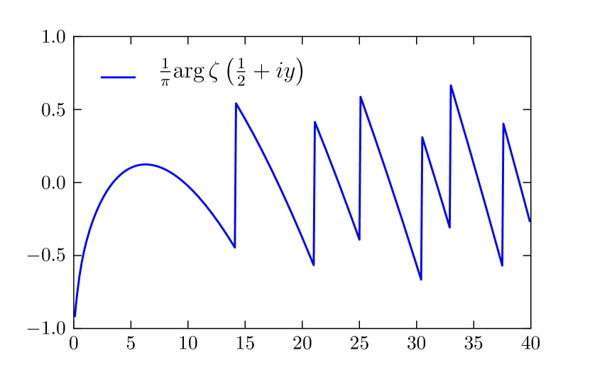
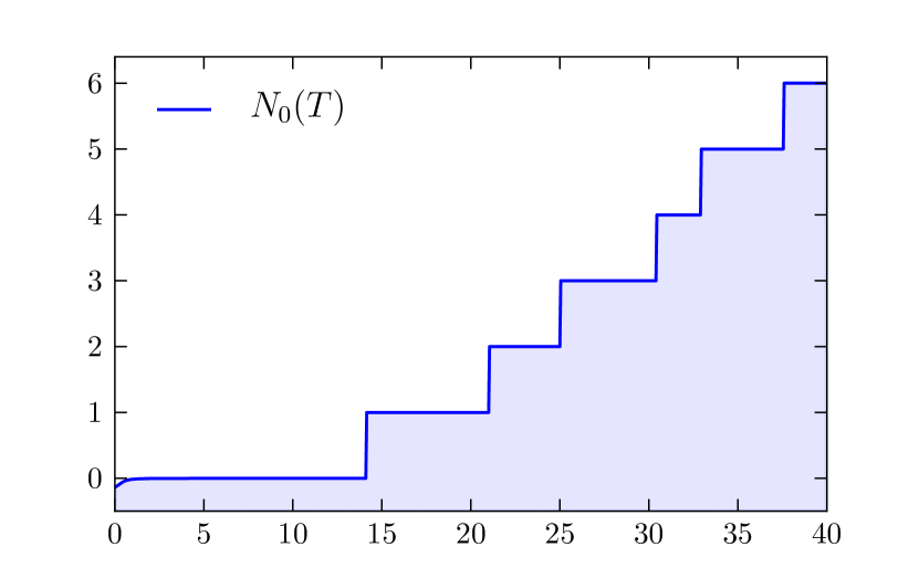
Figure 12: Left: $\tfrac{1}{\pi}\arg\zeta\left(\tfrac{1}{2}+iy\right)$ versus $y$, showing its rapid oscillation. The jumps occur on a Riemann zero. Right: $N_{0}(T)$ versus $T$ in (132), which is indistinguishable from a manual counting of zeros.

The reason $\delta$ needs to be positive in (138) is the following. Near a zero $\rho_{n}$,

$$\zeta(z)\approx\left(z-\rho_{n}\right)\zeta^{\prime}\left(\rho_{n}\right)=\left(\delta+i\left(y-y_{n}\right)\right)\zeta^{\prime}\left(\rho_{n}\right).$$ (128)

This gives

$$\arg\zeta(z)\approx\arctan\left((y-y_{n})/\delta\right)+\arg\zeta^{\prime}(\rho_{n}).$$ (129)

Thus, with $\delta>0$, as one passes through a zero from below, $S(y)$ increases by one, as it should based on its role in the counting formula $N(T)$. On the other hand, if $\delta<0$ then $S(y)$ would decrease by one instead.

We can now obtain a precise equation for the location of the zeros on the critical line. The equation (126), implies $\lim_{\delta\to 0^{+}}\theta\left(\tfrac{1}{2}+\delta,y\right)=\left(n+\tfrac{1}{2}\right)\pi$, for $n=0,\pm 1,\pm 2,\dotsc$, hence

$$n=\dfrac{y}{2\pi}\log\left(\dfrac{y}{2\pi e}\right)-\dfrac{5}{8}+\lim_{\delta\to 0^{+}}\dfrac{1}{\pi}\arg\zeta\left(\tfrac{1}{2}+\delta+iy\right).$$ (130)

A closer inspection shows that the RHS of the above equation has a minimum in the interval $(-2,-1)$, thus $n$ is bounded from below, i.e. $n\geq-1$. Establishing the convention that zeros are labeled by positive integers, $\rho_{n}=\tfrac{1}{2}+iy_{n}$ where $n=1,2,\dotsc$, we must replace $n\to n-2$ in (130). Therefore, the imaginary parts of these zeros satisfy the transcendental equation

$$\dfrac{y_{n}}{2\pi}\log\left(\dfrac{y_{n}}{2\pi e}\right)+\lim_{\delta\to 0^{+}}\dfrac{1}{\pi}\arg\zeta\left(\tfrac{1}{2}+\delta+iy_{n}\right)=n-\dfrac{11}{8}\qquad(n=1,2,\dotsc).$$ (131)

In summary, we have shown that, asymptotically for now, there are an infinite number of zeros on the critical line whose ordinates can be determined by solving (131). This equation determines the zeros on the upper half of the critical line. The zeros on the lower half are symmetrically distributed; if $\rho_{n}=\tfrac{1}{2}+iy_{n}$ is a zero, so is $\rho_{n}^{*}=\tfrac{1}{2}-iy_{n}$.

The LHS of (131) is a monotonically increasing function of $y$, and the leading term is a smooth function. This is clear since the same terms appear in the staircase function $N(T)$ described below. Possible discontinuities can only come from $\tfrac{1}{\pi}\arg\zeta\left(\tfrac{1}{2}+iy\right)$, and in fact, it has a jump discontinuity by one whenever $y$ corresponds to a zero on the line. However, if $\lim_{\delta\to 0^{+}}\arg\zeta\left(\tfrac{1}{2}+\delta+iy\right)$ is well defined for every $y$, then the left hand side of equation (131) is well defined for any $y$, and due to its monotonicity, there must be a unique solution for every $n$. Under this assumption, the number of solutions of equation (131), up to height $T$, is given by

$$N_{0}(T)=\dfrac{T}{2\pi}\log\left(\dfrac{T}{2\pi e}\right)+\dfrac{7}{8}+\dfrac{1}{\pi}\arg\zeta\left(\tfrac{1}{2}+iT\right)+O\left(T^{-1}\right).$$ (132)

This is so because the zeros are already numbered in (131), but the left hand side jumps by one at each zero, with values $-\tfrac{1}{2}$ to the left and $+\tfrac{1}{2}$ to the right of the zero. Thus we can replace $n\to N_{0}+\tfrac{1}{2}$ and $y_{n}\to T$, such that the jumps correspond to integer values. In this way $T$ will not correspond to the ordinate of a zero and $\delta$ can be eliminated.

Using Cauchy’s argument principle (see Appendix B) one can derive the Riemann-von Mangoldt formula, which gives the number of zeros in the region $\{0<x<1,\,0<y<T\}$ inside the critical strip. This formula is standard Edwards ; Titchmarsh :

$$N(T)=\dfrac{T}{2\pi}\log\left(\dfrac{T}{2\pi e}\right)+\dfrac{7}{8}+S(T)+O\left(T^{-1}\right).$$ (133)

The leading $T\log T$ term was already in Riemann’s original paper. Note that it has the same form as the counting formula on the critical line that we have just found (132). Thus, under the assumptions we have described, we conclude that $N_{0}(T)=N(T)$ asymptotically. This means that our particular solution (150), leading to equation (131), already saturates the counting formula on the whole strip and there are no additional zeros from $A=0$ in (145) nor from the more general equation $\theta+\theta^{\prime}=(2n+1)\pi$ described below. This strongly suggests that (131) describes all non-trivial zeros of $\zeta(z)$, which must then lie on the critical line.

VII.2 Exact equation satisfied by the $n$-th zero on the critical line

Let us now repeat the previous analysis but without considering an asymptotic expansion. The exact versions of (120) and (121) are

$$A(x,y) =\pi^{-x/2}|\Gamma\left(\tfrac{1}{2}(x+iy)\right)||\zeta(x+iy)|,$$ (134)

$$\theta(x,y) =\arg\Gamma\left(\tfrac{1}{2}(x+iy)\right)-\dfrac{y}{2}\log\pi+\arg\zeta(x+iy),$$ (135)

Then, as before, zeros are described by $\lim_{\delta\to 0^{+}}\cos\theta=0$, which is equivalent to $\lim_{\delta\to 0^{+}}\theta\left(\tfrac{1}{2}+\delta,y\right)=\left(n+\tfrac{1}{2}\right)\pi$, and replacing $n\to n-2$, the imaginary parts of these zeros must satisfy the exact equation

$$\arg\Gamma\left(\tfrac{1}{4}+\tfrac{i}{2}y_{n}\right)-y_{n}\log\sqrt{\pi}+\lim_{\delta\to 0^{+}}\arg\zeta\left(\tfrac{1}{2}+\delta+iy_{n}\right)=\left(n-\tfrac{3}{2}\right)\pi.$$ (136)

The Riemann-Siegel $\vartheta$ function is defined by

$$\vartheta(y)\equiv\arg\Gamma\left(\tfrac{1}{4}+\tfrac{i}{2}y\right)-y\log\sqrt{\pi},$$ (137)

where the argument is defined such that this function is continuous and $\vartheta(0)=0$. This can be done through the relation $\arg\Gamma=\Im\log\Gamma$, and numerically one can use the implementation of the “logGamma” function. This is equivalent to the analytic multivalued $\log\left(\Gamma\right)$ function, but it simplifies its complicated branch cut structure. Therefore, there are an infinite number of zeros in the form $\rho_{n}=\tfrac{1}{2}+iy_{n}$, where $n=1,2,\dotsc$, whose imaginary parts exactly satisfy the following equation:

$$\vartheta(y_{n})+\lim_{\delta\to 0^{+}}\arg\zeta\left(\tfrac{1}{2}+\delta+iy_{n}\right)=\left(n-\tfrac{3}{2}\right)\pi\qquad(n=1,2,\dotsc).$$ (138)

Expanding the $\Gamma$-function in (137) through Stirling’s formula

$$\vartheta(y)=\dfrac{y}{2}\log\left(\dfrac{y}{2\pi e}\right)-\dfrac{\pi}{8}+O(1/y)$$ (139)

one recovers the asymptotic equation (131).

Again, as discussed after (131), the first term in (138) is smooth and the whole left hand side is a monotonically increasing function. If $\lim_{\delta\to 0^{+}}\zeta\left(\tfrac{1}{2}+\delta+iy\right)$ is well defined for every $y$, then equation (138) must have a unique solution for every $n$. Under this condition it is valid to replace $y_{n}\to T$ and $n\to N_{0}+\tfrac{1}{2}$, and then the number of solutions of (138) is given by

$$N_{0}(T)=\dfrac{1}{\pi}\vartheta(T)+1+\dfrac{1}{\pi}\arg\zeta\left(\tfrac{1}{2}+iT\right).$$ (140)

The exact Backlund counting formula (see Appendix B), which gives the number of zeros on the critical strip with $0<\Im(\rho)<T$, is given by Edwards

$$N(T)=\dfrac{1}{\pi}\vartheta(T)+1+S\left(T\right).$$ (141)

Therefore, comparing (140) with the exact counting formula on the entire critical strip (141), we have $N_{0}(T)=N(T)$ exactly. This indicates that our particular solution, leading to equation (138), captures all the zeros on the strip, indicating that they should all be on the critical line.

In summary, if (138) has a unique solution for each $n$, then this saturates the counting formula for the entire critical strip and this would establish the validity of the RH.

VII.3 A more general equation

The above equation (138) was first obtained by us with a different argument RHLeclair ; FL1 . It is a particular solution of a more general formula which we now present.

We will need the following. From (115) we have $\left(\chi(z)\right)^{*}=\chi\left(z^{*}\right)$, thus $A(x,-y)=A(x,y)$ and $\theta(x,-y)=-\theta(x,y)$. Denoting

$$\chi\left(1-z\right)=A^{\prime}\,e^{-i\theta^{\prime}}$$ (142)

we then have

$$A^{\prime}(x,y)=A(1-x,y),\qquad\theta^{\prime}(x,y)=\theta(1-x,y).$$ (143)

From (116) we also have $|\chi(z)|=|\chi(1-z)|$, therefore

$$A(x,y)=A^{\prime}(x,y)$$ (144)

for any $z$ on the critical strip.

From (116) we see that if $\rho$ is a zero so is $1-\rho$. Then we clearly have

$$\lim_{z\to\rho}\left\{\chi(z)+\chi(1-z)\right\}=\lim_{z\to\rho}A(x,y)\,B(x,y)=0,$$ (145)

where we have defined

$$B(x,y)=e^{i\theta(x,y)}+e^{-i\theta^{\prime}(x,y)}.$$ (146)

The second equality in (145) follows from (144). For now, we do not specify the precise curve ${\cal C}$ through which we approach the zero.

The above equation (145) is identically satisfied on a zero $\rho$ since $\lim_{z\to\rho}A\sim|\zeta(\rho)|=0$, independently of $B$. However, this by itself does not provide any more detailed information on the zeros. There is much more information in the phases $\theta$ and $\theta^{\prime}$. Consider instead taking the limits in $A$ and $B$ separately,

$$\lim_{z^{\prime}\to\rho}\,\lim_{z\to\rho}\,A(x^{\prime},y^{\prime})\,B(x,y)=0,$$ (147)

where $z^{\prime}=x^{\prime}+iy^{\prime}$. Taking $z\to\rho$ first, a potential zero occurs when

$$\lim_{z\to\rho}B(x,y)=\lim_{z\to\rho}\left(e^{i\theta}+e^{-i\theta^{\prime}}\right)=0.$$ (148)

We propose that Riemann zeros satisfy (148). The equation $B=0$ provides more information on the location of zeros than $A=0$ since the phases $\theta$ and $\theta^{\prime}$ can be well defined at a zero through an appropriate limit. We emphasize that we have not yet assumed the RH, and the above analysis is valid on the entire complex plane, except at $z=1$ due to the simple pole of $\chi$. We will provide ample evidence that the equation (148) is evidently correct even for the example of the Davenport-Heilbronn function, which has zeros off the critical line, and the RH fails. Clearly a more rigorous derivation would be desirable, the delicacy being the limits involved, but let us proceed.

The linear combination in (145) was chosen to be manifestly symmetric under $z\to 1-z$. Had we taken a different linear combination in (145), such as $\chi(\rho)+b\,\chi(1-\rho)$, then $B=e^{i\theta}+b\,e^{-i\theta^{\prime}}$ for some constant $b$. Setting the real and imaginary parts of $B$ to zero gives the two equations $\cos\theta+b\cos\theta^{\prime}=0$ and $\sin\theta-b\sin\theta^{\prime}=0$. Summing the squares of these equations one obtains $\cos(\theta+\theta^{\prime})=-(b+1/b)/2$. However, since $b+1/b>1$, there are no solutions except for $b=1$.

The general solution of (148) is given by

$$\theta+\theta^{\prime}=(2n+1)\pi.$$ (149)

Note that $\chi(z)=\chi(1-z)$ implies $\theta+\theta^{\prime}=2\pi n$ for $z\neq\rho$. This together with (149) is analogous to the previous discussion where $\cos\theta=1$ for $z\neq\rho$ and $\cos\theta=0$ for $z=\rho$. All zeros satisfying (149) are simple since there are in correspondence with zeros of the cosine or sine function.

The zeros on the critical line correspond to the particular solution

$$\theta=\theta^{\prime}=(n+\tfrac{1}{2})\pi,$$ (150)

which is equivalent to (126) and (138).

In fact, the trivial zeros along the negative $x$ axis also satisfy (149), which again strongly supports its validity. One can show this as follows. For $x<0$, $\theta^{\prime}(x,0)=0$. Since we are on the real line, we approach the zero through the path $z=\rho-i\epsilon$, with $0<\epsilon\ll 1$. This path smooths out the $\arg\zeta$ term in the same way as the $\delta\to 0^{+}$ for zeros on the critical line. Then from (149) we are left with

$$\dfrac{1}{\pi}\theta(x,0)=\dfrac{1}{\pi}\Im\left[\log\Gamma\left(x/2\right)\right]+\dfrac{1}{\pi}\lim_{\epsilon\to 0^{+}}{\rm Arg}\,\zeta(x-i\epsilon)+2k=2n+1.$$ (151)

Note that we write $\arg\zeta(x-i\epsilon)={\rm Arg}\,\zeta(x-i\epsilon)+2\pi k$, where we have the principal value ${\rm Arg}\,\zeta(x)\in\{0,\pm\pi\}$ for $x<0$. The changes in branch are accounted for by $k$, and depend on $x$. If we take these changes correctly into account we obtain Figure 13, showing the trivial zeros as solutions to (151). The first term in (151), i.e. $\tfrac{1}{\pi}\Im\left[\log\Gamma(x/2)\right]$, is already a staircase function with jumps by $1$ at every negative even $x$. The other two terms, $\tfrac{1}{\pi}{\rm Arg}\,\zeta(x-i\epsilon)+2k$, just shift the function by a constant, such that these jumps coincide with odd integers $(2n+1)$ in such a way that (151) is satisfied exactly at a zero. Thus, remarkably the equation (149) characterizes all known zeros of $\zeta$.

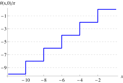
Figure 13: Plot of equation (151). Note the jumps occuring at $2n+1$ corresponding to the trivial zeros of the $\zeta$-function.

VII.4 On possible zeros off of the line

Suppose one looks for solutions to (149) off the line. In Figure 13 (right) we plot the RHS of (149) divided by $\pi$ for a region on the critical strip. One clearly sees that precisely where a solution requires that this equals an odd integer, the function is not well-defined. On the other hand, for $x=1/2$ with the $\delta$-prescription it is well-defined and has a unique solution.

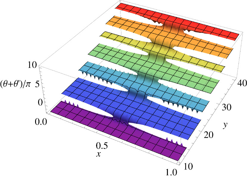
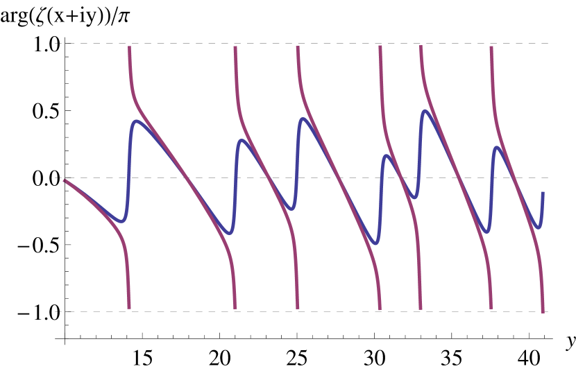
Figure 14: Left: $3D$ plot of $\tfrac{1}{\pi}\left[\theta(x,y)+\theta^{\prime}(x,y)\right]$. The function does not vary with $x$ on each plateau, but it is only well defined between jumps very close to the critical line. Right: $\tfrac{1}{\pi}\arg\zeta(x+iy)$ for $x=1/2+0.1$ (blue) and $x=1/2-0.1$ (purple) as a function of $y$.

The fact that the RHS of (149) is not well defined for $x>1/2$ is due to the very different properties of $\arg\zeta(x+iy)$ for $x>1/2$ verses $x<1/2$. In Figure 14 (right) we plot $\arg\zeta(x+iy)$ for $x=1/2\pm 0.1$ as a function of $y$. One sees that for $x<1/2$ there are severe changes of branch where the function is not defined, whereas for $x>1/2$ it is smooth. Since the RHS of (149) involves both $\theta$ and $\theta^{\prime}$, the $\theta^{\prime}$ term is ill-defined for $x>1/2$ and thus neither is the RHS. Only on the critical line where $\theta=\theta^{\prime}$ and $x=1/2+\delta$ with $\delta\to 0^{+}$ is the RHS well-defined.

There is another very interesting aspect of Figure 14 (left). On each plateau the function is mainly constant with respect to $x$. This formally follows from

$$\partial_{x}\left[\theta(x,y)+\theta^{\prime}(x,y)\right]=0$$ (152)

if one assumes $\theta$ is differentiable at $x$. This leads to the following suggestion. Suppose that the dependence on $x$ for $1/2<x\leq 1$ is weak enough that $\theta+\theta^{\prime}$ is very well approximated by the curve at $x=1$. Recall that it is known that there are no zeros along the line $x=1$. If the curve for $1/2<x<1$ is a smooth and very small deformation of the one at $x=1$, then there are no solutions to (149) off of the line, and if the latter captures all zeros, then there are no zeros off the line. As in section VI, the RH would then be related to the non-existence of zeros at $x=1$, which is equivalent to the prime number theorem. The main problem with this argument is that at a zero off the line, probably the above derivative is not well defined.

One sees that the particular solution (150) of the more general $B=0$ is a consequence of the direction in which the zero on the line is approached. Let $\zeta(z)=u(x,y)+iv(x,y)$ as in Section VI. The $u,v=\mbox{const.}$ contours are sketched in Figure 8. In the transcendental equation (136) the $\delta\to 0^{+}$ limit approaches the zero on the critical line along $u=0$ contours that are nearly in the $x$ direction. For potential zeros off of the line where $u,v=0$ contours intersect perpendicularly, one does not expect that the directions of these contours at the zeros is always the same, in contrast to those of the zeros on the critical line. Thus, for zeros off of the line, we expect $B=0$ will be satisfied, i.e. (149), but not the particular solution $\cos\theta=0$.

In Section XIX we will study an example of an $L$-series that does not satisfy the RH, the Davenport-Heilbronn function. We will show that the zeros off the line indeed satisfy (149).

VII.5 Further remarks

It is possible to introduce a new function $\zeta(z)\to\widetilde{\zeta}(z)=f(z)\zeta(z)$ that also satisfies the functional equation (116), i.e. $\widetilde{\chi}(z)=\widetilde{\chi}(1-z)$, but has zeros off of the critical line due to the zeros of $f(z)$. In such a case the corresponding functional equation will hold if and only if $f(z)=f(1-z)$ for any $z$, and this is a trivial condition on $f(z)$, which could have been canceled in the first place. Moreover, if $f(z)$ and $\zeta(z)$ have different zeros, the analog of equation (145) has a factor $f(z)$, i.e. $\widetilde{\chi}(\rho+\delta)+\widetilde{\chi}(1-\rho-\delta)=f(\rho+\delta)\left[\chi(\rho+\delta)+\chi(1-\rho-\delta)\right]=0$, implying (145) again where $\chi(z)$ is the original (115). Therefore, the previous analysis eliminates $f(z)$ automatically and only finds the zeros of $\chi(z)$. The analysis is non-trivial precisely because $\zeta(z)$ satisfies the functional equation but $\zeta(z)\neq\zeta(1-z)$. Furthermore, it is a well known theorem that the only function which satisfies the functional equation (116) and has the same characteristics of $\zeta(z)$, is $\zeta(z)$ itself. In other words, if $\widetilde{\zeta}(z)$ is required to have the same properties of $\zeta(z)$, then $\widetilde{\zeta}(z)=C\,\zeta(z)$, where $C$ is a constant (Titchmarsh, , pg. 31).

Although equations (138) and (141) have an obvious resemblance, it is impossible to derive the former from the later, since the later is just a counting formula valid on the entire strip, and it is assumed that $T$ is not the ordinate of a zero. Moreover, this would require the assumption of the validity of the RH, contrary to our approach, where we derived equations (138) and (131) on the critical line, without assuming the RH. Despite our best efforts, we were not able to find equations (131) and (138) in the literature. Furthermore, the counting formulas (132) and (141) have never been proven to be valid on the critical line Edwards .

VIII The argument of the Riemann $\zeta$-function

Let us recall the definition used in section VII, namely

$$S(y)=\lim_{\delta\to 0^{+}}\dfrac{1}{\pi}\arg\zeta\left(\tfrac{1}{2}+\delta+iy\right)=\lim_{\delta\to 0^{+}}\dfrac{1}{\pi}\Im\left[\log\zeta\left(\tfrac{1}{2}+\delta+iy\right)\right]).$$ (153)

Previously, we argued that $S(y_{n})$ is well defined at a zero $\rho=\tfrac{1}{2}+iy_{n}$ in the non-zero $\delta\to 0^{+}$ limit. A proper understanding of this function is essential in any theory of the Riemann zeros because of its role in the counting function $N(T)$, and in our equation (138) satisfied by individual zeros. It is the fluctuations in $S(y)$ that “knows” about the actual zeros. As stated above, if the equation (138) has a unique solution for every $n$, then the RH would follow since then $N_{0}(T)=N(T)$. In this section we describe some important properties of $S(y)$, the aim being to establish the latter. Some of these properties are known (see for instance Karatsuba ). Other properties we cannot prove but only provide heuristic arguments and numerical evidence.

The conventional way to define $S(y)$ is by piecewise integration of $\zeta^{\prime}/\zeta$ from $z=2$ to $2+iy$, then to $1/2+iy$. Namely $\arg\zeta(\tfrac{1}{2}+iy)=\arg\zeta(2+iy)+\Delta$, where $\Delta=\arg\zeta(\tfrac{1}{2}+iy)-\arg\zeta(2+iy)$. The integration to arbitrarily high $y$ along $\Re(z)=2$ is bounded and gives something relatively small on the principal branch. This can be seen from the Euler product. For $x>1$,

$$\arg\zeta(x+iy)=\Im\log\zeta(x+iy)=\dfrac{1}{2i}\sum_{p}\log\left(\dfrac{1-p^{-x+iy}}{1-p^{-x-iy}}\right)\approx-\sum_{p}\dfrac{1}{p^{x}}\sin(y\log p).$$ (154)

For $x=2$,

$$|\arg\zeta(2+iy)|<\sum_{p=}\dfrac{1}{p^{2}}=0.452235\dotsc.$$ (155)

The above sum obviously converges since it is less than $\zeta(2)=\pi^{2}/6=1.645$.

One often sees statements in the literature such as $S(y)=O(\log y)$. Such a logarithmic growth could only come from the short integration that gives $\Delta$ of the last paragraph, which is curious since there is no such growth in $|\arg\zeta(2+iy)|$. Assuming the RH, the current best bound is given by

$$|S(y)|\leq\left(\tfrac{1}{2}+o(1)\right)\tfrac{\log y}{\log\log y}$$

for $y\to\infty$, proven by Goldston and Gonek Goldston . It is important to bear in mind that these are upper bounds, and that $S(y)$ may actually be much smaller. In fact, there is no numerical evidence for such a logarithmic growth. Even in his own paper, Riemann writes the correction to the smooth part of $N(T)$ as $O(1/T)$ rather than $O(\log T)$. Our own studies, and the arguments below, lead us to propose actually that $S(y)=O(1)$, and that it is nearly always on the principle branch, i.e. $-1<S(y)<1$. Some, but not all, of our arguments are limited to the region where the RH is known to be true, which about up to the $10^{9}$-th zero, namely $0<y<3.7\times 10^{8}$.

The first three properties of $S(y)$ listed below are well-known Edwards ; Titchmarsh ; Karatsuba :

1. At each zero $\rho=x+iy$ in the critical strip, $S(y)$ jumps by the multiplicity $m$ of the zero. This simply follows from the role of $S(T)$ in the counting formula $N(T)$ in (141). For instance, simple zeros on the critical line have $m=1$, whereas double zeros on the line have $m=2$. Since zeros off the line at a given height $y$ always occurs in pairs, i.e. $\rho$ and $1-\rho^{*}$, if one of such zeros has multiplicity $m$, then $S(y)$ has to jump by $2m$ at this height $y$. It is believed that all the Riemann zeros are simple, although this is largely a completely open problem.

2. Between zeros, since $N(y)$ is constant,

   $$S^{\prime}(y)=\partial_{y}S(y)=-\dfrac{1}{\pi}\vartheta^{\prime}(y)<0,$$ (156)

   where the last inequality follows because $\vartheta(y)$ is a monotonically increasing function.

3. The average $\langle S\rangle$ of $S(y)$ is zero Edwards ,

   $$\langle S\rangle=\lim_{Y\to\infty}\dfrac{1}{Y}\int_{0}^{Y}dy\,S(y)=0.$$ (157)

4. Let

   $$\Delta S_{n}\equiv S(y_{n})-S(y_{n+1})=\dfrac{1}{\pi}\left(\vartheta(y_{n+1})-\vartheta(y_{n})\right)$$ (158)

   where the equality follows from (156). Then, if the RH is true, $\Delta S_{n}$ has to compensate the jumps by $1$ at each zero, and since $\langle S\rangle=0$, one has

   $$\langle\Delta S_{n}\rangle=1.$$ (159)

There is one more property we will need, which is a precise statement of the fact that the real part of $\zeta(\tfrac{1}{2}+iy)$ is almost always positive. Let $y^{(+)}_{n}$ and $y^{(-)}_{n}$, where $n=1,2,\dotsc$, denote the points where either the imaginary or real part, respectively, of $\zeta(1/2+iy)$ are zero, but not both. These points are easy to find since they do not depend on the fluctuating $S(y)$. We have

$$\zeta(\tfrac{1}{2}-iy)=\zeta\left(\tfrac{1}{2}+iy\right)\,G(y),\qquad G(y)=e^{2i\vartheta(y)}$$ (160)

where $\vartheta(y)$ is the smooth Riemann-Siegel function (137). Since the real and imaginary parts are not both zero, at $y^{(+)}_{n}$ then $G=1$, whereas at $y^{(-)}_{n}$ then $G=-1$. Thus

$$\Im\left[\zeta\left(\tfrac{1}{2}+iy^{(+)}_{n}\right)\right] =0 \mbox{for}\ \vartheta(y^{(+)}_{n}) =(n-1)\pi,$$ (161)

$$\Re\left[\zeta\left(\tfrac{1}{2}+iy^{(-)}_{n}\right)\right] =0 \mbox{for}\ \vartheta(y^{(-)}_{n}) =\left(n-\tfrac{1}{2}\right)\pi.$$ (162)

Our convention is $n=1$ for the first point where this occurs for $y>0$. Using the approximation (139), equations (161) and (162) can be written in the form $\tfrac{y}{2\pi}\log\left(\tfrac{y}{2\pi e}\right)=A_{n}$, which through the transformation $y\to 2\pi A_{n}x^{-1}$ can be solved in terms of the Lambert $W$-function (see Section XII). The result is

$$y_{n}^{(+)}=\dfrac{2\pi\left(n-7/8\right)}{W\left[e^{-1}(n-7/8)\right]},\qquad y_{n}^{(-)}=\dfrac{2\pi\left(n-3/8\right)}{W\left[e^{-1}(n-3/8)\right]},$$ (163)

where above $n=1,2,\dotsc$ and $W$ denotes the principal branch $W_{0}$. The $y^{(+)}_{n}$ are actually the Gram points. From (163) we can see that these points are ordered in a regular manner,

$$y^{(+)}_{1}<y^{(-)}_{1}<y^{(+)}_{2}<y^{(-)}_{2}<y^{(+)}_{3}<y^{(-)}_{3}<\dotsm$$ (164)

as illustrated in Figure 15 (left).

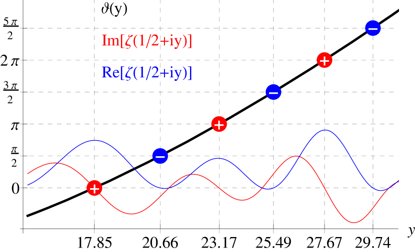
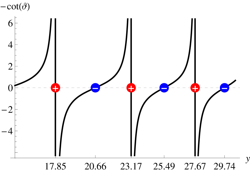
Figure 15: Left: the $y_{n}^{(+)}$ (red balls) are the Gram points, where $\Im\left[\zeta\left(\tfrac{1}{2}+iy\right)\right]=0$, and $y_{n}^{(-)}$ (blue balls) are the points where $\Re\left[\zeta\left(\tfrac{1}{2}+iy\right)\right]=0$. These points are determined from formulas (163). Right: A plot of (165) indicating the points (163).

The ratio

$$\dfrac{\Re\left[\zeta\left(\tfrac{1}{2}+iy\right)\right]}{\Im\left[\zeta\left(\tfrac{1}{2}+iy\right)\right]}=-\cot\vartheta(y)$$ (165)

has a regular repeating pattern, as can be seen in Figure 15 (right), thus the signs of the real and imaginary parts are related in a specific manner. From this figure one sees that when the imaginary part is negative the real part is positive, suggesting that the phase of the function stays mainly in the principal branch.

1. The statement we need about the real part being mainly positive concerns the average value of the real part at the points $y^{(+)}_{n}$. The average of the real part of $\zeta\left(\tfrac{1}{2}+iy\right)$ at the Gram points $y^{(+)}_{n}$ is Titchmarsh

   $$\lim_{N\to\infty}\dfrac{1}{N}\sum_{n=1}^{N}\Re\left[\zeta\left(\tfrac{1}{2}+iy^{(+)}_{n}\right)\right]=2.$$ (166)

Now, let us consider the behavior of $S(y)$ starting from the first zero. At the first zero, in the jump by $1$, $S(y)$ passes through zero and remains on the principle branch (see Figure 12). The branch cut in the $z$-plane is along the negative $x$-axis, thus on the principle branch $-1<S(y)\leq 1$. At the points $y^{(+)}_{n}$, where the imaginary part is zero, the vast majority of them have $\Re\big{[}\zeta\big{(}\tfrac{1}{2}+iy^{(+)}_{n}\big{)}\big{]}>0$ according to item 5 above, and thus for the most part $S(y^{(+)}_{n})=0$. Thus $S(y)=0$ at infinitely many points $y^{(+)}_{n}$ between zeros, consistent with $\langle S\rangle=0$.

At the relatively rare points $y^{(+)}_{n}$ where $\Re\big{[}\zeta\big{(}\tfrac{1}{2}+iy^{(+)}_{n}\big{)}\big{]}<0$, $S(y)$ crosses one of the lines $S(y)=\pm 1$. Taking into account the properties 5 and 4, one concludes that $S(y)$ primarily stays in the principle branch, i.e. it can pass to another branch, but it quickly returns to the principal branch. An example where this occurs is close to the point $y^{(+)}_{127}=282.455$. The function starts to change branch, and as soon as it crosses the branch cut, there is a Riemann zero at $y_{127}=282.465$ so $S(y)$ jumps by $1$ coming back to the principal branch again. This behavior is shown Figure 16 and one sees that $S(y)$ just barely touches $-1$.

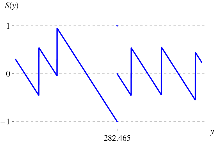
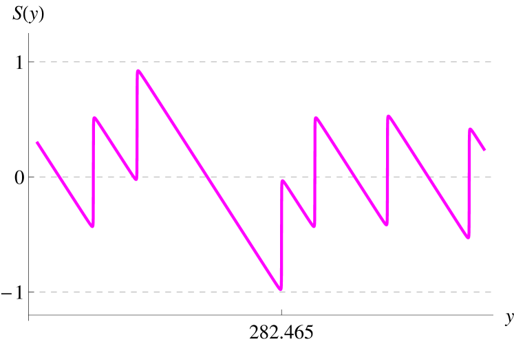
Figure 16: Left: $S(y)$ in the vicinity of the first point where $|S(y)|>1$, at $y^{(+)}_{127}=282.455$. There is a zero at $y_{127}=282.465$. Right: by adding a $\delta$ in $S(y)=\tfrac{1}{\pi}\arg\zeta\left(\tfrac{1}{2}+\delta+iy\right)$ we can smooth out the curve such that it stays in the principal branch.

In Figure 17 (left) we plot $S(y)$ on the principle branch in the vicinity of another point where $S(y)$ passes to another branch. This time it passes to another branch while jumping at the zero $y_{1018}=1439.623$. The real part is negative for $y^{(+)}_{1017}=1439.778$. Since $S^{\prime}(y)<0$ it comes back to the principal branch pretty quickly. The interpretation of this figure is that $S(y)$ has changed branch: the dangling part of the curve at the bottom should be shifted by $2$ to make $S(y)$ continuous. By including a $\delta$ we can smooth out the curve to make it continuous and to stay in the principal branch, as shown in Figure 17 (right), and this is a better rendition of the actual behavior.

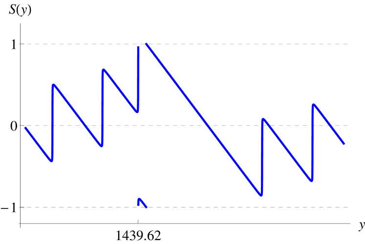
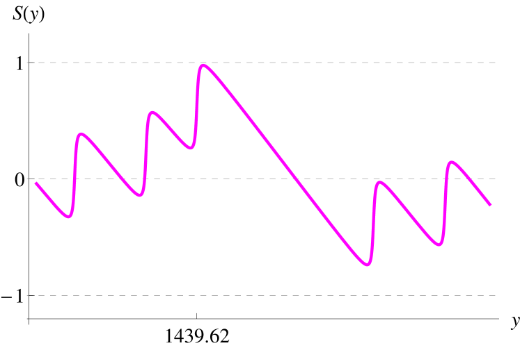
Figure 17: Left: $S(y)$ on the principle branch in the vicinity of $y^{(+)}_{1017}=1439.778$ where $S(y)>1$. Right: we have included a non-zero $\delta$ to smooth out the function, and it stays in the principal branch.

Note that at the rare points where $|S(y)|\geq 1$, it strays off the principle branch but quickly returns to it. In Figure 18 (left) we plot $S(y)$ around the $10^{5}$-th zero, and one sees that it is still on the principle branch. In contrast consider the hypothetical behavior sketched in Figure 18 (right). Many oscillations around $|S|=1$ are potentially in conflict with property 5 since it requires many points $y^{(+)}_{n}$ where the real part is negative. Furthermore, in order to maintain $\langle S\rangle=0$, there must be some large values of $\Delta S_{n}$, in potential conflict with (159). The situation is even worse if there indeed are zeros off of the critical line. In such a case $S(y)$ would jump by at least $2$ and it is not clear if it would eventually decrease fast enough to come back to the principal branch. Of course one cannot rule out such a hypothetical behavior in some high region of the critical line, but it is seems very unlikely.

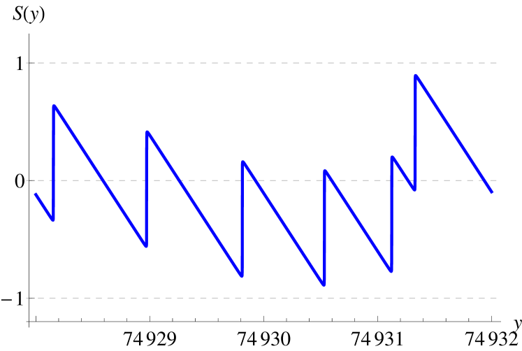
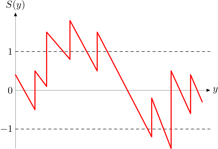
Figure 18: Left: behavior of $S(y)$ around the $10^{5}$-th zero. Right: an unlikely hypothetical behavior of $S(y)$.

In summary, although we are unable to rigorously prove it, we have given arguments suggesting that $S(y)$ is nearly always on the principle branch, i.e. almost always $|S(y)|<1$. Furthermore, the small $\delta$ in (153) makes $S(y)$ well defined and smooth as shown in Figures 16 and 17 (right). This is the property that we need to be able to solve equation (138). Up to the height about the $10^{9}$-th zero, this property was well satisfied. This numerical analysis will be presented below. In this range we see absolutely no evidence for a logarithmic growth of $S(y)$. In short, it is these properties of $S(y)$ that we believe are responsible for the existence of a unique solution to the equation (138) for any $n$.

The above arguments show that most of the time $S(y)$ passes through zero at each jump by one. We present two conjectures on the average of $S(y)$ at the zeros. The first is

$$\lim_{N\to\infty}\dfrac{1}{N}\sum_{n=1}^{N}S(y_{n})=0$$ (167)

This is closely related to $\langle S\rangle=0$. Much more interesting is the average of the absolute value of $S(y)$ at the zeros, which we call the “bounce number” and denote it by $b$. If $S(y_{n})$ is on the principle branch, then $|S(y_{n})|<1$ and

$$b_{N}=\dfrac{1}{N}\sum_{n=1}^{N}|S(y_{n})|<1.$$ (168)

Also, clearly $\lim_{N\to\infty}b_{N+1}/b_{N}=1$. Therefore

$$b=\lim_{N\to\infty}b_{N}$$ (169)

is well-defined. On average the absolute value of $S(y)$ on a zero should be less than $1/2$ since $S(y)$ passes through zero at most of the jumps by $1$. The most symmetric result would be $b=1/4$, but due to the rare changes of branch described above, we expect $1/4<b<1/2$. Numerically, for the first million zeros we find a value just above $1/4$:

$$b_{N}=0.264\qquad\mbox{for $N=10^{6}$.}$$ (170)

The bounce number $b$ contains important information about the multiplicity of zeros. Many jumps in $S(y)$ with multiplicity $m\geq 2$ would clearly raise $b$ to a significantly higher value.

There is a well-known counter example to the RH based on the Davenport-Heilbronn function. It has a functional equation like $\zeta$, but is known to have zeros off of the critical line. We will study this function in Section XIX, and explain how the properties of $S(y)$ described in this section are violated. In short, at a zero off of the line there is a change of branch in such a manner that the analog of $S(y)$ is ill defined, and there is thus no solution to the transcendental equation at these points, so the argument that $N_{0}(T)=N(T)$ fails.

IX Zeros of Dirichlet $L$-functions

IX.1 Some properties of Dirichlet $L$-functions

We now consider the generalization of the previous results for the $\zeta$-function to Dirichlet $L$-functions. The main arguments are the same as for $\zeta$, thus we do not repeat all of the statements in Section VII.

Much less is known about the zeros of $L$-functions in comparison with the $\zeta$-function, however let us mention a few works. Selberg Selberg1 obtained the analog of Riemann-von Mangoldt counting formula (133) for Dirichlet $L$-functions. Based on this result, Fujii Fujii gave an estimate for the number of zeros on the critical strip with the ordinate between $[T+H,T]$. The distribution of low lying zeros of $L$-functions near and at the critical line was examined in Iwaniec , assuming the generalized Riemann hypothesis (GRH). The statistics of the zeros, i.e. the analog of the Montgomery-Odlyzko conjecture, were studied in Conrey3 ; Hughes . It is also known that more than half of the non-trivial zeros of Dirichlet $L$-functions are on the critical line Conrey4 . For a more detailed introduction to $L$-functions see Bombieri2 .

Let us first introduce the basic ingredients and definitions regarding this class of functions, which are all well known Apostol . Dirichlet $L$-series are defined as

$$L(z,\chi)=\sum_{n=1}^{\infty}\dfrac{\chi(n)}{n^{z}}\qquad(\Re(z)>1)$$ (171)

where the arithmetic function $\chi(n)$ is a Dirichlet character. They enjoy an Euler product formula

$$L(z,\chi)=\prod_{p}\dfrac{1}{1-\chi(p)\,p^{-z}}\qquad\left(Re(z)>1\right).$$ (172)

They can all be analytically continued to the entire complex plane, except for a simple pole at $z=1$, and are then referred to as Dirichlet $L$-functions.

There are an infinite number of distinct Dirichlet characters which are primarily characterized by their modulus $k$, which determines their periodicity. They can be defined axiomatically, which leads to specific properties, some of which we now describe. Consider a Dirichlet character $\chi$ mod $k$, and let the symbol $(n,k)$ denote the greatest common divisor of the two integers $n$ and $k$. Then $\chi$ has the following properties:

1. $\chi(n+k)=\chi(n)$.

2. $\chi(1)=1$ and $\chi(0)=0$.

3. $\chi(nm)=\chi(n)\chi(m)$.

4. $\chi(n)=0$ if $(n,k)>1$ and $\chi(n)\neq 0$ if $(n,k)=1$.

5. If $(n,k)=1$ then $\chi(n)^{\varphi(k)}=1$, where $\varphi(k)$ is the Euler totient arithmetic function. This implies that $\chi(n)$ are roots of unity.

6. If $\chi$ is a Dirichlet character so is the complex conjugate $\chi^{*}$.

For a given modulus $k$ there are $\varphi(k)$ distinct Dirichlet characters, which essentially follows from property 5 above. They can thus be labeled as $\chi_{k,j}$ where $j=1,2,\dotsc,\varphi(k)$ denotes an arbitrary ordering. If $k=1$ we have the trivial character where $\chi(n)=1$ for every $n$, and (171) reduces to the Riemann $\zeta$-function. The principal character, usually denoted by $\chi_{1}$, is defined as $\chi_{1}(n)=1$ if $(n,k)=1$ and zero otherwise. In the above notation the principal character is always $\chi_{k,1}$.

Characters can be classified as primitive or non-primitive. Consider the Gauss sum

$$G(\chi)=\sum_{m=1}^{k}\chi(m)e^{2\pi im/k}.$$ (173)

If the character $\chi$ mod $k$ is primitive, then

$$|G(\chi)|^{2}=k.$$ (174)

This is no longer valid for a non-primitive character. Consider a non-primitive character $\overline{\chi}$ mod $\overline{k}$. Then it can be expressed in terms of a primitive character of smaller modulus as $\overline{\chi}(n)=\overline{\chi_{1}}(n)\chi(n)$, where $\overline{\chi_{1}}$ is the principal character mod $\overline{k}$ and $\chi$ is a primitive character mod $k<\overline{k}$, where $k$ is a divisor of $\overline{k}$. More precisely, $k$ must be the conductor of $\overline{\chi}$ (see Apostol for further details). In this case the two $L$-functions are related as $L(z,\overline{\chi})=L(z,\chi)\Pi_{p|\overline{k}}\left(1-\chi(p)/p^{z}\right)$. Thus $L(z,\overline{\chi})$ has the same zeros as $L(z,\chi)$. The principal character is only primitive when $k=1$, which yields the $\zeta$-function. The simplest example of non-primitive characters are all the principal ones for $k\geq 2$, whose zeros are the same as the $\zeta$-function. Let us consider another example with $\overline{k}=6$, where $\varphi(6)=2$, namely $\overline{\chi}_{6,2}$, whose components are

$$n$$

(175)

In this case, the only divisors are $2$ and $3$. Since $\chi_{1}$ mod $2$ is non-primitive, it is excluded. We are left with $k=3$ which is the conductor of $\overline{\chi}_{6,2}$. Then we have two options; $\chi_{3,1}$ which is the non-primitive principal character mod $3$, thus excluded, and $\chi_{3,2}$ which is primitive. Its components are

$$n$$

(176)

Note that $|G(\chi_{6,2})|^{2}=3\neq 6$ and $|G(\chi_{3,2})|^{2}=3$. In fact one can check that $\overline{\chi}_{6,2}(n)=\overline{\chi}_{6,1}(n)\chi_{3,2}(n)$, where $\overline{\chi}_{6,1}$ is the principal character mod $\overline{k}=6$. Thus the zeros of $L(z,\overline{\chi}_{6,2})$ are the same as those of $L(z,\chi_{3,2})$. Therefore, it suffices to consider primitive characters, and we will henceforth do so.

We will need the functional equation satisfied by $L(z,\chi)$. Let $\chi$ be a primitive character. Define its order $a$ such that

$$a\equiv\begin{cases}1&\mbox{if $\chi(-1)=-1$ (odd),}\\ 0&\mbox{if $\chi(-1)=1$ (even).}\end{cases}$$ (177)

Let us define the meromorphic function

$$\Lambda(z,\chi)\equiv\left(\dfrac{k}{\pi}\right)^{\tfrac{z+a}{2}}\Gamma\left(\dfrac{z+a}{2}\right)L(z,\chi).$$ (178)

Then $\Lambda$ satisfies the well known functional equation Apostol

$$\Lambda(z,\chi)=\dfrac{i^{-a}\,G(\chi)}{\sqrt{k}}\,\Lambda(1-z,\chi^{*}).$$ (179)

The above equation is only valid for primitive characters.

IX.2 Exact equation for the $n$-th zero

For a primitive character, since $|G(\chi)|=\sqrt{k}$, the factor on the right hand side of (179) is a phase. It is thus possible to obtain a more symmetric form through a new function defined as

$$\xi(z,\chi)\equiv\dfrac{i^{a/2}\,k^{1/4}}{\sqrt{G\left(\chi\right)}}\,\,\Lambda(z,\chi).$$ (180)

It then satisfies

$$\xi(z,\chi)=\xi^{*}(1-z,\chi)\equiv\left(\xi(1-z^{*},\chi)\right)^{*}.$$ (181)

Above, the function $\xi^{*}$ of $z$ is defined as the complex conjugation of all coefficients that define $\xi$, namely $\chi$ and the $i^{a/2}$ factor, evaluated at a non-conjugated $z$.

Note that $(\Lambda(z,\chi))^{*}=\Lambda(z^{*},\chi^{*})$. Using the well known result

$$G\left(\chi^{*}\right)=\chi(-1)\left(G(\chi)\right)^{*}$$ (182)

we conclude that

$$\left(\xi(z,\chi)\right)^{*}=\xi\left(z^{*},\chi^{*}\right).$$ (183)

This implies that if the character is real, then if $\rho$ is a zero of $\xi$ so is $\rho^{*}$, and one needs only consider $\rho$ with positive imaginary part. On the other hand if $\chi\neq\chi^{*}$, then the zeros with negative imaginary part are different than $\rho^{*}$. For the trivial character where $k=1$ and $a=0$, implying $\chi(n)=1$ for any $n$, then $L(z,\chi)$ reduces to the Riemann $\zeta$-function and (181) yields the well known functional equation (116).

Let $z=x+iy$. Then the function (180) can be written as

$$\xi(z,\chi)=Ae^{i\theta}$$ (184)

where

$$A(x,y,\chi) =\left(\dfrac{k}{\pi}\right)^{\tfrac{x+a}{2}}\left|\Gamma\left(\dfrac{x+a+iy}{2}\right)\right|\left|L(x+iy,\chi)\right|,$$ (185)

$$\theta(x,y,\chi) =\arg\Gamma\left(\dfrac{x+a+iy}{2}\right)-\dfrac{y}{2}\log\left(\dfrac{\pi}{k}\right)-\dfrac{1}{2}\arg G(\chi)+\arg L(x+iy,\chi)+\dfrac{\pi a}{4}.$$ (186)

From (183) we also conclude that $A(x,y,\chi)=A(x,-y,\chi^{*})$ and $\theta(x,y,\chi)=-\theta(x,-y,\chi^{*})$. Denoting

$$\xi^{*}(1-z,\chi)=A^{\prime}e^{-i\theta^{\prime}}$$ (187)

we have

$$A^{\prime}(x,y,\chi)=A(1-x,y,\chi),\qquad\theta^{\prime}(x,y,\chi)=\theta(1-x,y,\chi).$$ (188)

Taking the modulus of (181) we also have that $A(x,y,\chi)=A^{\prime}(x,y,\chi)$ for any $z$.

On the critical strip, the functions $L(z,\chi)$ and $\xi(z,\chi)$ have the same zeros. Thus on a zero we clearly have

$$\lim_{z\to\rho}\left\{\xi(z,\chi)+\xi^{*}(1-z,\chi)\right\}=0.$$ (189)

Let us define

$$B(x,y,\chi)\equiv e^{i\theta(x,y,\chi)}+e^{-i\theta^{\prime}(x,y,\chi)}.$$ (190)

Since $A=A^{\prime}$ everywhere, and taking separate limits in (189) we therefore have

$$\lim_{z^{\prime}\to\rho}\lim_{z\to\rho}A(x^{\prime},y^{\prime},\chi)\,B(x,y,\chi)=0.$$ (191)

Considering the $z\to\rho$ limit, a potential zero occurs when

$$\lim_{z\to\rho}B(x,y,\chi)=0.$$ (192)

The general solution of this equation is thus given by

$$\theta+\theta^{\prime}=(2n+1)\pi.$$ (193)

Until now, the path to approach the zero $z\to\rho$ was not specified. Now we put ourselves on the critical line $x=1/2$, and the path will be choosen as $z=\rho+\delta$ with $0<\delta\ll 1$. Then $\theta=\theta^{\prime}$ and (193) yields

$$\lim_{\delta\to 0^{+}}\theta\left(\tfrac{1}{2}+\delta,y\right)=\left(n+\tfrac{1}{2}\right)\pi.$$ (194)

Let us define the function

$$\vartheta_{k,a}(y)\equiv\Im\left[\log\Gamma\left(\dfrac{1}{4}+\dfrac{a}{2}+i\,\dfrac{y}{2}\right)\right]-\dfrac{y}{2}\log\left(\dfrac{\pi}{k}\right).$$ (195)

When $k=1$ and $a=0$, the function (195) is just the usual Riemann-Siegel $\vartheta$ function (137). Thus (194) gives the equation

$$\vartheta_{k,a}(y_{n})+\lim_{\delta\to 0^{+}}\arg L\left(\tfrac{1}{2}+\delta+iy_{n},\chi\right)-\dfrac{1}{2}\arg G\left(\chi\right)+\dfrac{\pi a}{4}=\left(n+\dfrac{1}{2}\right)\pi.$$ (196)

Analyzing the left hand side of (196) we can see that it has a minimum, thus we shift $n\to n-(n_{0}+1)$ for a given $n_{0}$, to label the zeros according to the convention that the first positive zero is labelled by $n=1$. Thus the upper half of the critical line will have the zeros labelled by $n=1,2,\dotsc$ corresponding to positive $y_{n}$, while the lower half will have the negative values $y_{n}$ labelled by $n=0,-1,\dotsc$. The integer $n_{0}$ depends on $k$, $a$ and $\chi$, and should be chosen according to each specific case. In the cases we analyze below $n_{0}=0$, whereas for the trivial character $n_{0}=1$. In practice, the value of $n_{0}$ can always be determined by plotting (196) with $n=1$, passing all terms to its left hand side. Then it is trivial to adjust the integer $n_{0}$ such that the graph passes through the point $(y_{1},0)$ for the first jump, corresponding to the first positive solution. Henceforth we will omit the integer $n_{0}$ in the equations, since all cases analyzed in the following have $n_{0}=0$. Nevertheless, the reader should bear in mind that for other cases, it may be necessary to replace $n\to n-n_{0}$ in the following equations.

In summary, these zeros have the form $\rho_{n}=\tfrac{1}{2}+iy_{n}$, where for a given $n\in\mathbb{Z}$, the imaginary part $y_{n}$ is the solution of the equation

$$\vartheta_{k,a}(y_{n})+\lim_{\delta\to 0^{+}}\arg L\left(\tfrac{1}{2}+\delta+iy_{n},\chi\right)-\dfrac{1}{2}\arg G\left(\chi\right)=\left(n-\dfrac{1}{2}-\dfrac{a}{4}\right)\pi.$$ (197)

IX.3 Asymptotic equation for the $n$-th zero

From Stirling’s formula we have the following asymptotic form for $y\to\pm\infty$:

$$\vartheta_{k,a}(y)=\mathrm{sgn}(y)\left(\dfrac{|y|}{2}\log\left(\dfrac{k|y|}{2\pi e}\right)+\dfrac{2a-1}{8}\pi+O(1/y)\right).$$ (198)

The first order approximation of (197), i.e. neglecting terms of $O(1/y)$, is given by

$$\sigma_{n}\dfrac{|y_{n}|}{2\pi}\log\left(\dfrac{k\,|y_{n}|}{2\pi e}\right)+\dfrac{1}{\pi}\lim_{\delta\to 0^{+}}\arg L\left(\tfrac{1}{2}+\delta+i\sigma_{n}|y_{n}|,\chi\right)-\dfrac{1}{2\pi}\arg G\left(\chi\right)=\alpha_{n},$$ (199)

where

$$\alpha_{n}=n+\dfrac{\sigma_{n}-4-2a(1+\sigma_{n})}{8}.$$ (200)

Above $\sigma_{n}=1$ if $n>0$ and $\sigma_{n}=-1$ if $n\leq 0$. For $n>0$ we have $y_{n}=|y_{n}|$ and for $n\leq 0$ $y_{n}=-|y_{n}|$.

IX.4 Counting formulas

Let us define $N^{+}_{0}(T,\chi)$ as the number of zeros on the critical line with $0<\Im(\rho)<T$ and $N^{-}_{0}(T,\chi)$ as the number of zeros with $-T<\Im(\rho)<0$. As explained before, $N^{+}_{0}(T,\chi)\neq N^{-}_{0}(T,\chi)$ if the characters are complex numbers, since the zeros are not symmetrically distributed between the upper and lower half of the critical line.

The counting formula $N^{+}_{0}(T,\chi)$ is obtained from (197) by replacing $y_{n}\to T$ and $n\to N^{+}_{0}+1/2$, therefore

$$N^{+}_{0}(T,\chi)=\dfrac{1}{\pi}\vartheta_{k,a}(T)+\dfrac{1}{\pi}\arg L\left(\tfrac{1}{2}+iT,\chi\right)-\dfrac{1}{2\pi}\arg G\left(\chi\right)+\dfrac{a}{4}.$$ (201)

The passage from (197) to (201) is justified under the assumptions already discussed in connection with (132) and (140), i.e. assuming that (197) has a unique solution for every $n$. Analogously, the counting formula on the lower half line is given by

$$N_{0}^{-}(T,\chi)=\dfrac{1}{\pi}\vartheta_{k,a}(T)-\dfrac{1}{\pi}\arg L\left(\tfrac{1}{2}-iT,\chi\right)+\dfrac{1}{2\pi}\arg G(\chi)-\dfrac{a}{4}.$$ (202)

Note that in (201) and (202) $T$ is positive. Both cases are plotted in Figure 19 for the character $\chi_{7,2}$ shown in (238). One can notice that they are precisely staircase functions, jumping by one at each zero. Note also that the functions are not symmetric about the origin, since for a complex $\chi$ the zeros on upper and lower half lines are not simply complex conjugates.

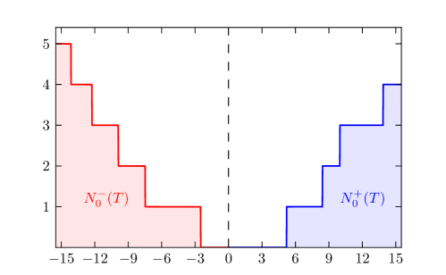
Figure 19: Exact counting formulae (201) and (202). Note that they are not symmetric with respect to the origin, since the $L$-zeros for complex $\chi$ are not complex conjugates. We used $\chi=\chi_{7,2}$ (238).

From (198) we also have the first order approximation for $T\to\infty$,

$$N^{+}_{0}(T,\chi)=\dfrac{T}{2\pi}\log\left(\dfrac{k\,T}{2\pi e}\right)+\dfrac{1}{\pi}\arg L\left(\tfrac{1}{2}+iT,\chi\right)-\dfrac{1}{2\pi}\arg G\left(\chi\right)-\dfrac{1}{8}+\dfrac{a}{2}.$$ (203)

Analogously, for the lower half line we have

$$N^{-}_{0}(T,\chi)=\dfrac{T}{2\pi}\log\left(\dfrac{k\,T}{2\pi e}\right)-\dfrac{1}{\pi}\arg L\left(\tfrac{1}{2}-iT,\chi\right)+\dfrac{1}{2\pi}\arg G\left(\chi\right)-\dfrac{1}{8}.$$ (204)

As in (197), again we are omitting $n_{0}$ since in the cases below $n_{0}=0$, but for other cases one may need to include $\pm n_{0}$ on the right hand side of $N_{0}^{\pm}$, respectively.

It is known that the number of zeros on the entire critical strip up to height $T$, i.e. in the region $\{0<x<1,\,0<y<T\}$, is given by Montgomery

$$N^{+}(T,\chi)=\dfrac{1}{\pi}\vartheta_{k,a}\left(T\right)+\dfrac{1}{\pi}\arg L\left(\tfrac{1}{2}+iT,\chi\right)-\dfrac{1}{\pi}\arg L\left(\tfrac{1}{2},\chi\right).$$ (205)

This formula follows from a straightforward generalization of the method shown in Appendix B for the $\zeta$-function. From Stirling’s approximation and using

$$2a-1=-\chi(-1),$$ (206)

for $T\to\infty$ we obtain the asymptotic approximation Selberg1 ; Montgomery

$$N^{+}(T,\chi)=\dfrac{T}{2\pi}\log\left(\dfrac{k\,T}{2\pi e}\right)+\dfrac{1}{\pi}\arg L\left(\tfrac{1}{2}+iT,\chi\right)-\dfrac{1}{\pi}\arg L\left(\tfrac{1}{2},\chi\right)-\dfrac{\chi(-1)}{8}+O(1/T).$$ (207)

Both formulas (205) and (207) are exactly the same as (201) and (203), respectively. This can be seen as follows. From (181) we conclude that $\xi$ is real on the critical line. Thus

$$\arg\xi\left(\tfrac{1}{2}\right)=0=-\dfrac{1}{2}\arg G\left(\chi\right)+\arg L\left(\tfrac{1}{2},\chi\right)+\dfrac{\pi a}{4}.$$ (208)

Then, replacing $\arg G$ in (197) we obtain

$$\vartheta_{k,a}\left(y_{n}\right)+\lim_{\delta\to 0^{+}}\arg L\left(\tfrac{1}{2}+\delta+iy_{n},\chi\right)-\arg L\left(\tfrac{1}{2},\chi\right)=\left(n-\tfrac{1}{2}\right)\pi.$$ (209)

Replacing $y_{n}\to T$ and $n\to N_{0}^{+}+1/2$ in (209) we have precisely the expression (205), and also (207) for $T\to\infty$. Therefore, we conclude that $N_{0}^{+}(T,\chi)=N^{+}(T,\chi)$ exactly. From (183) we see that negative zeros for character $\chi$ correspond to positive zeros for character $\chi^{*}$. Then for $-T<\Im(\rho)<0$ the counting on the strip also coincides with the counting on the line, since $N_{0}^{-}(T,\chi)=N_{0}^{+}(T,\chi^{*})$ and $N^{-}(T,\chi)=N^{+}(T,\chi^{*})$. Therefore, the number of zeros on the whole critical strip is the same as the number of zeros on the critical line obtained as solutions of (197). This is valid under the assumption that (197) has a unique solution for every $n$.

X Zeros of $L$-functions based on modular forms

Let us generalize the previous results to $L$-functions based on level one modular forms. We first recall some basic definitions and properties. The modular group can be represented by the set of $2\times 2$ integer matrices

$$SL_{2}\left(\mathbb{Z}\right)=\left\{A=\begin{pmatrix}a&b\\ c&d\end{pmatrix}\,\big{|}\,\,a,b,c,d\in\mathbb{Z},\ \det A=1\right\},$$ (210)

provided each matrix $A$ is identified with $-A$, i.e. $\pm A$ are regarded as the same transformation. Thus for $\tau$ in the upper half complex plane, it transforms as

$$\tau\mapsto A\tau=\dfrac{a\tau+b}{c\tau+d}$$

under the action of the modular group. A modular form $f$ of weight $k$ is a function that is analytic in the upper half complex plane which satisfies the functional relation Apostolmodular

$$f\left(\dfrac{a\tau+b}{c\tau+d}\right)=\left(c\tau+d\right)^{k}f(\tau).$$ (211)

If the above equation is satisfied for all of $SL_{2}\left(\mathbb{Z}\right)$, then $f$ is referred to as being of level one. It is possible to define higher level modular forms which satisfy the above equation for a subgroup of $SL_{2}\left(\mathbb{Z}\right)$. Since our results are easily generalized to the higher level case, henceforth we will only consider level one forms.

For the $SL_{2}\left(\mathbb{Z}\right)$ element $\big{(}\begin{smallmatrix}1&1\\ 0&1\end{smallmatrix}\big{)}$, the above implies the periodicity $f(\tau)=f(\tau+1)$, thus it has a Fourier series

$$f(\tau)=\sum_{n=0}^{\infty}a_{f}(n)\,q^{n},\qquad q\equiv e^{2\pi i\tau}.$$ (212)

If $a_{f}(0)=0$ then $f$ is called a cusp form.

From the Fourier coefficients, one can define the Dirichlet series

$$L_{f}\left(z\right)=\sum_{n=1}^{\infty}\dfrac{a_{f}\left(n\right)}{n^{z}}.$$ (213)

The functional equation relates $L_{f}\left(z\right)$ to $L_{f}\left(k-z\right)$, so that the critical line is $\Re(z)=k/2$, where $k\geq 4$ is an even integer. One can always shift the critical line to $1/2$ by replacing $a_{f}(n)\to a_{f}(n)/n^{(k-1)/2}$, however we will not do this here. Let us define

$$\Lambda_{f}(z)\equiv\left(2\pi\right)^{-z}\,\Gamma\left(z\right)\,L_{f}(z).$$ (214)

Then the functional equation is given by Apostolmodular

$$\Lambda_{f}(z)=(-1)^{k/2}\Lambda_{f}(k-z).$$ (215)

There are only two cases to consider since $k/2$ can be an even or an odd integer. As in (180) we can absorb the extra minus sign factor for the odd case. Thus we define $\xi_{f}(z)\equiv\Lambda_{f}(z)$ for $k/2$ even, and we have $\xi_{f}(z)=\xi_{f}(k-z)$, and $\xi_{f}(z)\equiv e^{-i\pi/2}\Lambda_{f}(z)$ for $k/2$ odd, implying $\xi_{f}(z)=\xi_{f}^{*}(k-z)$. Representing $\xi_{f}(z)=|\xi_{f}|\,e^{i\theta}$ where $z=x+iy$, we follow exactly the same steps as in the previous sections. From the solution (193) we conclude that there are infinite zeros on the critical line $\Re(\rho)=k/2$ determined by $\lim_{\delta\to 0^{+}}\theta\left(\tfrac{k}{2}+\delta,y,\chi\right)=\left(n-\tfrac{1}{2}\right)\pi$. Therefore, these zeros have the form $\rho_{n}=\tfrac{k}{2}+iy_{n}$, where $y_{n}$ is the solution of the equation

$$\vartheta_{k}(y_{n})+\lim_{\delta\to 0^{+}}\arg L_{f}\left(\tfrac{k}{2}+\delta+iy_{n}\right)=\left(n-\dfrac{1+(-1)^{k/2}}{4}\right)\pi$$ (216)

for $n=1,2,\dotsc$, and we have defined

$$\vartheta_{k}(y)\equiv\Im\left[\log\Gamma\left(\tfrac{k}{2}+iy\right)\right]-y\log 2\pi.$$ (217)

This implies that the number of solutions of (216) with $0<y<T$ is given by

$$N_{0}\left(T\right)=\dfrac{1}{\pi}\vartheta_{k}(T)+\dfrac{1}{\pi}\arg L_{f}\left(\tfrac{k}{2}+iT\right)-\dfrac{1-(-1)^{k/2}}{4}.$$ (218)

In the limit of large $y_{n}$, neglecting terms of $O(1/y)$, the equation (216) becomes

$$y_{n}\log\left(\dfrac{y_{n}}{2\pi e}\right)+\lim_{\delta\to 0^{+}}\arg L_{f}\left(\tfrac{k}{2}+\delta+iy_{n}\right)=\left(n-\dfrac{k+(-1)^{k/2}}{4}\right)\pi.$$ (219)

XI The Lambert $W$-function

The following section, and even more, section XX, will involve the Lambert-$W$ function, thus we review its most important properties in this section. The basic facts about the $W$-function that we present, including some history, are essentially based on Corless , where the reader can also find more details.

In $1758$ Lambert solved the equation $x=q+x^{m}$, expressing $x$, and also powers $x^{\alpha}$, as power series in $q$. A few years later Euler considered a more symmetric version of this equation through the substitution $x\to x^{-\beta}$, $q\to(\alpha-\beta)v$ and $m\to\tfrac{\alpha}{\beta}$. Then taking the limit $\beta\to\alpha$ one obtains $\log x=vx^{\alpha}$. This equation can be written in the form $\log x=vx$ through $x^{\alpha}\to x$ and $\alpha v\to v$. Thus, exponentiating the last equation and introducing the variables $z=-v$ and $W(z)=-vx$, we obtain the equation

$$W(z)\,e^{W(z)}=z.$$ (220)

$W(z)$ is called the Lambert function, and (220) is its defining equation. Although its power series approximation was consider for the first time by Lambert and Euler, this function only started to be effectively studied during the past $20$ years. The $W$-function should be considered as a new elementary function, since it cannot be expressed in terms of the other known elementary functions.

Johan Heinrich Lambert was born in Mulhouse (a French city making border with Switzerland and Germany) in $1728$, and died in Berlin in $1777$. Lambert was a self educated mathematician having a broad range of scientific interests. He contributed to number theory, geometry, statistics, astronomy, cosmology and philosophy, just to name a few areas. He is responsible for the modern notation of hyperbolic functions, and was the first one to prove the irrationality of $\pi$. When Euler considered the solution to equation $\log x=vx$, he gave credit to Lambert. The translation of his paper’s title is “On a series of Lambert and some of its significant properties”. It seems that Euler learned about Lambert’s result from a conversation between both when Lambert was travelling from Zürich to Berlin. Euler described his excitement in a letter to Goldbach in 1764.

Leaving history aside, let us now consider the $W$-function defined through (220) over a complex field, $z\in\mathbb{C}$. $W(z)$ is not a single-valued function, so we need to introduce its branch structure. This is done following the same branch structure of $\log z$, that we now recall. If $u=\log z$ then for every $z$ we have $e^{u}=z$. However, note that $u$ is not uniquely defined since $u\to u+2\pi ki$ for $k\in\mathbb{Z}$ will give the same $z$. Thus it is necessary to divide the complex $u$-plane in regions which are single-valued related to the $z$-plane. Each of these regions is called a branch and is labelled by $k$. The way one partitions the $u$-plane is a convention. The most convenient way is to define the $k$-th branch as the region on the $u$-plane limited by

$$(2k-1)\pi<\Im(u)\leq(2k+1)\pi,\qquad k\in\mathbb{Z}.$$ (221)

Each boundary in (221) is mapped on the negative real line $(-\infty,0]$ of the $z$-plane. The line $(-\infty,0]$ is called the branch cut and $z=0$ is the branch point. We adopt the counterclockwise direction such that the branch cut closes on top, i.e. for $z=re^{i\theta}$, $-\pi<\theta\leq\pi$ then $\log z$, for each branch $k$, is a continuous function of $z$.

Now let us turn back to $W(z)$. We refer to the $W$-plane and the $z$-plane, and denote

$$W=u+iv,\qquad z=x+iy.$$ (222)

From the defining equation (220) we have

$$x=e^{u}\left(u\cos v-v\sin v\right),\qquad y=e^{u}\left(u\sin v+v\cos v\right).$$ (223)

We require the branch cut of $W(z)$ to be similar to $\log z$, thus we define the branch cut on the $z$-plane to be the line $(-\infty,0]$. Imposing $y=0$ and $x\leq 0$ on relations (223) we obtain the boundaries and regions shown in Figure 20 (left). Thus the boundaries of each branch are given by the curves which are contained in the shaded regions, which are shown in Figure 20 (right). Each of these lines are mapped to the branch cut $(-\infty,0]$ in the $z$-plane. For each branch $k$ the lower boundary is open, and not included, while the upper boundary is closed, and included, in its defining region. From now on we denote $W(z)$ by $W_{k}(z)$ when referring to the specific $k$-th branch. Note that the boundary lines are asymptotic to $W=n\pi i$.

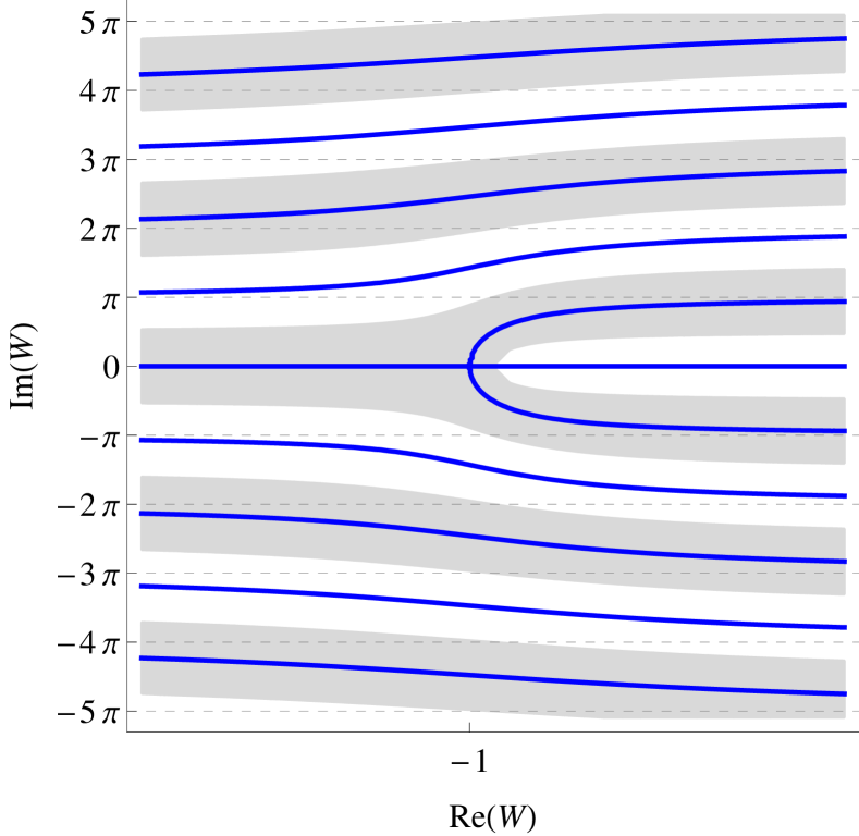
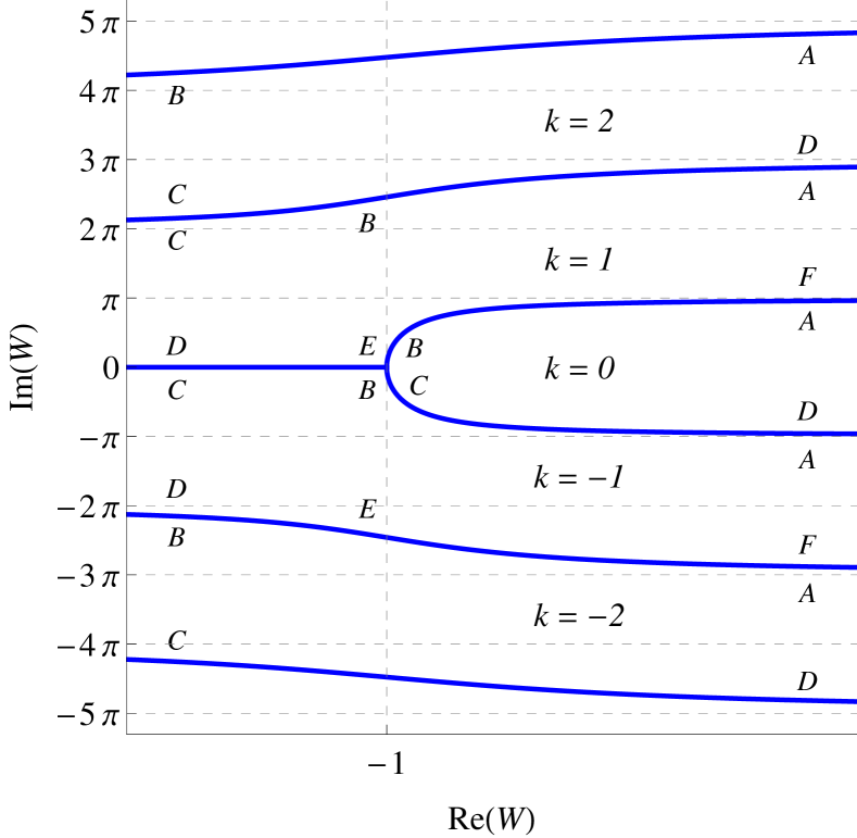
Figure 20: Left: the solid (blue) lines correspond to the condition $y=0$ in (223) and the shaded (gray) regions to $x\leq 0$. Right: the boundaries of each branch are given by the lines which are contained in the shaded regions. This is the branch structure of $W(z)$ viewed from the $W$-plane.

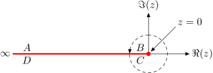
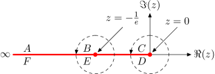
Figure 21: Left: Mapping from $W_{k}$ for $k=\pm 2,\pm 3,\dotsc$ (Figure 20 (right)) into the $z$-plane. Note how the points $A,\,B,\,C\,$ and $D$ are mapped. We close the contour on top, i.e. $z=re^{i\theta}$ where $-\pi<\theta\leq\pi$, and $W_{k}(z)$ is a continuous single-valued function. Right: The branch cuts for $W_{\pm 1}$.

The branches $W_{k}$ for $k=\pm 2,\pm 3,\dotsc$ in Figure 20 (right) are mapped into the $z$-plane according to Figure 21 (left). The curve in the $W$-plane separating $W_{k}$ from $W_{k+1}$ for $k=1,2,\dotsc$ is given by $\left\{-v\cot v+iv\ |\ 2k\pi<v<(2k+1)\pi\right\}$, and the curve separating $W_{k}$ from $W_{k-1}$ for $k=-1,-2,\dotsc$ is given by $\left\{-v\cot v+iv\ |\ (2k-1)\pi<v<2k\pi\right\}$.

The branch structure for $W_{0}$ and $W_{\pm 1}$ is different from above. The curves shown in Figure 20 (right), separating $W_{0}$ from $W_{\pm 1}$ are given by $\left\{-v\cot v+iv\ |\ -\pi<v<\pi\right\}$. The point $W=-1$, corresponding to $z=-1/e$, is a double branch point, linking $W_{0}$ and $W_{\pm 1}$. The curve separating $W_{1}$ and $W_{-1}$ is $(-\infty,-1]$. Note that $W_{1}$ does not include the real line, since the lower boundary is not included in its region. The branches $W_{0}$ and $W_{-1}$ are special in the sense that they are the only ones which include part of the real line. Thus only $W_{0}$ and $W_{-1}$ can yield real values.

The branches $W_{1}$ and $W_{-1}$ have a double branch cut in the $z$-plane. One is the line $(-\infty,0]$ and the other is $(-\infty,-1/e]$. Both branches are mapped into the $z$-plane according to Figure 21 (right). Note how the points $A,\,B,\,\dotsc F$ are related.

The branch $W_{0}$ has only one branch cut which is $(-\infty,-1/e]$. It is exactly like in Figure 21 (left) but with the point $z=0$ replaced by $z=-1/e$. For real values of $z\in[-1/e,\infty)$ we see from (220) that $W_{0}(-1/e)=-1$, $W_{0}(0)=0$ and $W_{0}(\infty)=\infty$. For the branch $W_{-1}$ we see that the function is real for $z\in[-1/e,0)$, having the values $W_{-1}(-1/e)=-1$ and $W_{-1}(0)=-\infty$. Thus for real $z$ we have the picture shown in Figure 22. Sometimes the principal branch $W_{0}$ is denoted simply by $W$ for short, when there is no chance of confusion.

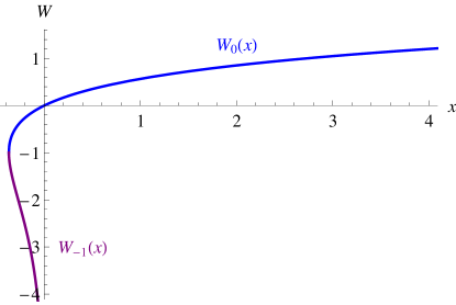
Figure 22: The two branches $W_{0}(x)$ and $W_{-1}(x)$ for real $x$. These are the only branches giving real values. The domain of $W_{0}(x)$ is $x\in[-1/e,\infty)$ and the domain of $W_{-1}(x)$ is $x\in[-1/e,0)$.

Now it only remains to show that each branch maps bijectively into the $z$-plane. This will be true provided the Jacobian determinant of the transformation (223) does not vanish. We therefore have

$$J=\dfrac{\partial(x,y)}{\partial(u,v)}=e^{u}\begin{pmatrix}\cos v+u\cos v-v\sin v&&-v\cos v-\sin v-u\sin v\\ \sin v+v\cos v+u\sin v&&\cos v+u\cos v-v\sin v\end{pmatrix}.$$ (224)

Then, $\det J=e^{2u}\left(v^{2}+(1+u)^{2}\right)$. This can only be zero if $u=-1$ and $v=0$, which correspond exactly to the double branch point. Thus for every branch $W_{k}$ we have $\det J>0$.

Except on the branch cut we have the symmetry

$$\left(W_{k}(z)\right)^{*}=W_{-k}\left(z^{*}\right).$$ (225)

This can easily be seen from Figure 20 (right), where the branches are symmetric by $v\to-v$, and analyzing how the points are mapped into the $z$-plane by complex conjugation on the $W$-plane.

XII Approximate zeros in terms of the Lambert $W$-function

XII.1 Explicit formula

We now show that it is possible to obtain an approximate solution to the previous transcendental equations with an explicit formula. Let us start with the zeros of the $\zeta$-function, described by equation (131). Consider its leading order approximation, or equivalently its average since $\langle\arg\zeta\left(\tfrac{1}{2}+iy\right)\rangle=0$. Then we have the transcendental equation

$$\dfrac{\widetilde{y}_{n}}{2\pi}\log\left(\dfrac{\widetilde{y}_{n}}{2\pi e}\right)=n-\dfrac{11}{8}.$$ (226)

Through the transformation

$$\widetilde{y}_{n}=2\pi\left(n-\dfrac{11}{8}\right)\dfrac{1}{x_{n}}$$ (227)

the equation (226) can be written as

$$x_{n}e^{x_{n}}=\dfrac{n-\tfrac{11}{8}}{e}.$$ (228)

Comparing with (220) we thus we obtain

$$\widetilde{y}_{n}=\dfrac{2\pi\left(n-\tfrac{11}{8}\right)}{W\left[e^{-1}\left(n-\tfrac{11}{8}\right)\right]}$$ (229)

for $n=1,2,\dotsc$, where above $W$ denotes the principal branch $W_{0}$.

Although the inversion from (226) to (229) is rather simple, it is very convenient since it is indeed an explicit formula depending only on $n$, and $W$ is included in most numerical packages. It gives an approximate solution for the ordinates of the Riemann zeros in closed form. The values computed from (229) are much closer to the Riemann zeros than Gram points, and one does not have to deal with violations of Gram’s law (see below).

Analogously, for Dirichlet $L$-functions, after neglecting the $\arg L$ term, the equation (199) yields a transcendental equation which can be solved explicitly as

$$\widetilde{y}_{n}=\dfrac{2\pi\sigma_{n}A_{n}\left(\chi\right)}{W\left[k\,e^{-1}A_{n}\left(\chi\right)\right]}$$ (230)

for $n=0,\pm 1,\pm 2,\dotsc$ and where

$$A_{n}\left(\chi\right)=\sigma_{n}\left(n+\dfrac{1}{2\pi}\arg G(\chi)\right)+\dfrac{1-4\sigma_{n}-2a\left(\sigma_{n}+1\right)}{8}.$$ (231)

In the above formula $n=1,2,\dotsc$ correspond to positive $y_{n}$ solutions, while $n=0,-1,\dotsc$ correspond to negative $y_{n}$ solutions. Contrary to the $\zeta$-function, in general, the zeros are not conjugate related along the critical line.

In the same way, ignoring the small $\arg L_{f}$ term in (219), the approximate solution for the imaginary part of the zeros of $L$-functions based on level one modular forms is given by

$$\widetilde{y}_{n}=\dfrac{A_{n}\pi}{W\left[(2e)^{-1}A_{n}\right]}$$ (232)

where $n=1,2,\dotsc$ and

$$A_{n}=n-\dfrac{k+(-1)^{k/2}}{4}.$$ (233)

XII.2 Further remarks

Let us focus on the approximation (229) regarding zeros of the $\zeta$-function. Obviously the same arguments apply to the zeros of the other classes of functions, based on formulas (230) and (232).

The estimates given by (229) can be calculated to high accuracy for arbitrarily large $n$, since $W$ is a standard elementary function. Of course, the $\widetilde{y}_{n}$ are not as accurate as the solutions $y_{n}$ including the $\arg\zeta$ term, as we will see in section XIII. Nevertheless, it is indeed a good estimate, especially if one considers very high zeros, where traditional methods have not previously estimated such high values. For instance, formula (229) can easily estimate the zeros shown in Table 1, and much higher if desirable.

$n$	$\widetilde{y}_{n}$
$10^{22}+1$	$1.370919909931995308226770\times 10^{21}$
$10^{50}$	$5.741532903784313725642221053588442131126693322343461\times 10^{48}$
$10^{100}$	$2.80690383842894069903195445838256400084548030162846045192360059224930$
	$922349073043060335653109252473234\times 10^{98}$
$10^{200}$	$1.38579222214678934084546680546715919012340245153870708183286835248393$
	$8909689796343076797639408172610028651791994879400728026863298840958091$
	$288304951600695814960962282888090054696215023267048447330585768\times 10^{198}$

Table 1: Formula (229) can easily estimate very high Riemann zeros. The results are expected to be correct up to the decimal point, i.e. to the number of digits in the integer part. The numbers are shown with three digits beyond the integer part.

The numbers in this table are accurate approximations to the $n$-th zero to the number of digits shown, which is approximately the number of digits in the integer part. For instance, the approximation to the $10^{100}$ zero is correct to $100$ digits. With Mathematica we easily calculated the first million digits of the $10^{10^{6}}$ zero.

Using the asymptotic behaviour $W(x)\sim\log x$ for large $x$, the $n$-th zero is approximately $\widetilde{y}_{n}\approx 2\pi n/\log n$, as already known Titchmarsh . The distance between consecutive zeros is $2\pi/\log n$, which tends to zero when $n\to\infty$.

The solutions (229) are reminiscent of the so-called Gram points $g_{n}$, which are solutions to $\vartheta(g_{n})=n\pi$ where $\vartheta$ is given by (137). Gram’s law is the tendency for Riemann zeros to lie between consecutive Gram points, but it is known to fail for about $1/4$ of all Gram intervals. Our $\widetilde{y}_{n}$ are intrinsically different from Gram points. It is an approximate solution for the ordinate of the zero itself. In particular, the Gram point $g_{0}=17.8455$ is the closest to the first Riemann zero, whereas $\widetilde{y}_{1}=14.52$ is already much closer to the true zero which is $y_{1}=14.1347\dotsc$. The traditional method to compute the zeros is based on the Riemann-Siegel formula, $\zeta\left(\tfrac{1}{2}+iy\right)=Z(y)\left(\cos\vartheta(y)-i\sin\vartheta(y)\right)$, and the empirical observation that the real part of this equation is almost always positive, except when Gram’s law fails, and $Z(y)$ has the opposite sign of $\sin\vartheta$. Since $Z(y)$ and $\zeta\left(\tfrac{1}{2}+iy\right)$ have the same zeros, one looks for the zeros of $Z(y)$ between two Gram points, as long as Gram’s law holds $(-1)^{n}Z\left(g_{n}\right)>0$. To verify the RH numerically, the counting formula (141) must also be used, to assure that the number of zeros on the critical line coincide with the number of zeros on the strip. The detailed procedure is throughly explained in Edwards ; Titchmarsh . Based on this method, amazingly accurate solutions and high zeros on the critical line were computed OdlyzkoSchonhage ; Odlyzko ; Odlyzko2 ; Gourdon . Nevertheless, our proposal is fundamentally different. We claim that (138), or its asymptotic approximation (131), is the equation that determines the Riemann zeros on the critical line. Then, one just needs to find its solution for a given $n$. We will compute the Riemann zeros in this way in the next section, just by solving the equation numerically, starting from the approximation given by the explicit formula (229), without using Gram points nor the Riemann-Siegel $Z$ function. Let us emphasize that our goal is not to provide a more efficient algorithm to compute the zeros OdlyzkoSchonhage , although the method described here may very well be, but to justify the validity of equations (131) and (138).

XIII Numerical analysis: $\zeta$-function

Instead of solving the exact equation (138) we will initially consider its first order approximation, which is equation (131). As we will see, this approximation already yields surprisingly accurate values for the Riemann zeros. These approximate solutions will be used to study the GUE statistics and prime number counting function in the next two sections.

Let us first consider how the approximate solution given by (229) is modified by the presence of the $\arg\zeta$ term in (131). Numerically, we compute $\arg\zeta$ taking its principal value. As already discussed, the function $\arg\zeta\left(\tfrac{1}{2}+iy\right)$ oscillates around zero, as shown in Figure 12 (left). At a zero it can be well-defined by the limit (123), which is generally not zero. For example, for the first Riemann zero $y_{1}=14.1347\dotsc$,

$$\lim_{\delta\to 0^{+}}\arg\zeta\left(\tfrac{1}{2}+\delta+iy_{1}\right)=0.157873919880941213041945.$$ (234)

The $\arg\zeta$ term plays an important role and indeed improves the estimate of the $n$-th zero. This can be seen in Figure 23, where we compare the estimate given by (229) with the numerical solutions of (131).

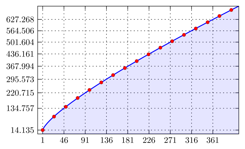
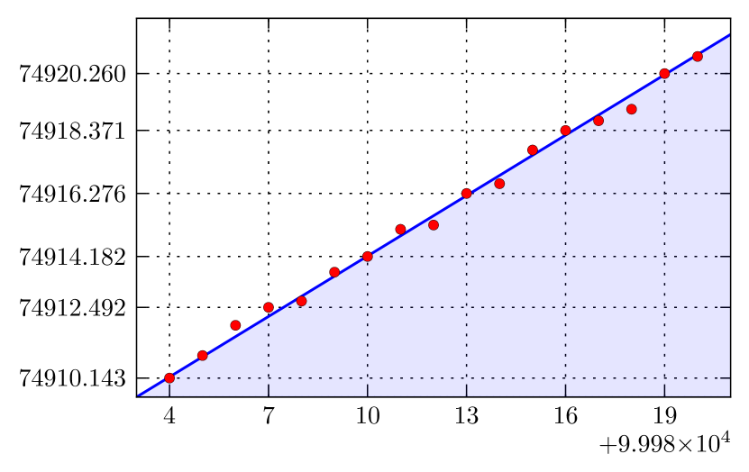
Figure 23: Comparison of (229) (blue line) and (131) (red dots). We plot $y_{n}$ against $n$. Left: here $n\in[1,\dotsc,400]$. Right: if we focus on a small range we can see the solutions of (131) oscillating around the line (229) due to the fluctuating $\arg\zeta$ term. Here $n\in[99984,\dotsc,10^{5}]$.

Since equation (131) typically alternates in sign around a zero, we can apply a root finder method in an appropriate interval, centered around the approximate solution $\widetilde{y}_{n}$ given by formula (229). Some of the solutions obtained in this way are presented in Table 2 (left), and are accurate up to the number of decimal places shown. We used only Mathematica or some very simple algorithms to perform these numerical computations, taken from standard open source numerical libraries.

$n$	$\widetilde{y}_{n}$	$y_{n}$
$1$	$14.52$	$14.134725142$
$10$	$50.23$	$49.773832478$
$10^{2}$	$235.99$	$236.524229666$
$10^{3}$	$1419.52$	$1419.422480946$
$10^{4}$	$9877.63$	$9877.782654006$
$10^{5}$	$74920.89$	$74920.827498994$
$10^{6}$	$600269.64$	$600269.677012445$
$10^{7}$	$4992381.11$	$4992381.014003179$
$10^{8}$	$42653549.77$	$42653549.760951554$
$10^{9}$	$371870204.05$	$371870203.837028053$
$10^{10}$	$3293531632.26$	$3293531632.397136704$

$n$	$y_{n}$
$1$	$14.13472514173469379045725198356247$
$2$	$21.02203963877155499262847959389690$
$3$	$25.01085758014568876321379099256282$
$4$	$30.42487612585951321031189753058409$
$5$	$32.93506158773918969066236896407490$
$6$	$37.58617815882567125721776348070533$
$7$	$40.91871901214749518739812691463325$
$8$	$43.32707328091499951949612216540681$
$9$	$48.00515088116715972794247274942752$
$10$	$49.77383247767230218191678467856372$
$11$	$52.97032147771446064414729660888099$

Table 2: Numerical solutions of equation (131). Left: solutions accurate up to the $9$-th decimal place and agree with Odlyzko ; Oliveira . Right: although it was derived for high $y$, it provides accurate numbers even for the lower zeros.

Although the formula for $y_{n}$ was solved for large $n$, it is surprisingly accurate even for the lower zeros, as shown in Table 2 (right). It is actually easier to solve numerically for low zeros since $\arg\zeta$ is better behaved. These numbers are correct up to the number of digits shown, and the precision was improved simply by decreasing the error tolerance.

XIV GUE statistics

The link between the Riemann zeros and random matrix theory started with the pair correlation of zeros, proposed by Montgomery Montgomery , and the observation of Dyson that it is the same as the $2$-point correlation function predicted by the gaussian unitary ensemble (GUE) for large random matrices Dyson .

The main result of the GUE random matrix theory is that the eigenvalues of a random hermitian matrix are not completely random, for instance there are correlations in the spacings of eigenvalues, commonly referred to as level-repulsion. In Figure 24 we show 3 collections of points: the first 50 Riemann zeros, $50$ random real numbers between 0 and the ordinate of the $50$-th zero, and the eigenvalues of a $50\times 50$ hermitian matrix where each element of the matrix is also random. One clearly sees the statistical resemblance of the statistics of the Riemann zeros and that of the GUE, in contrast to the $50$ random numbers.

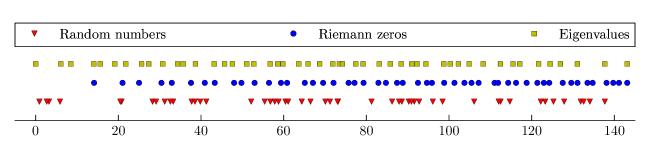
Figure 24: The first $50$ Riemann zeros at $x=1/2$, in comparison with $50$ random numbers to the left and the eigenvalues of a random $50\times 50$ hermitian matrix.

The main purpose of this section is to test whether our approximation (131) to the zeros is accurate enough to reveal this statistics. Whereas formula (229) is a valid estimate of the zeros, it is not sufficiently accurate to reproduce the GUE statistics, since it does not have the oscillatory $\arg\zeta$ term. On the other hand, the solutions to equation (131) are accurate enough, which again indicates the importance of the $\arg\zeta$ term.

Montgomery’s pair correlation conjecture can be stated as follows:

$$\dfrac{1}{N(T)}\sum_{\begin{subarray}{c}0\leq y,y^{\prime}\leq T\\[2.79996pt] \alpha<d(y,y^{\prime})\leq\beta\end{subarray}}1\ \sim\ \int_{\alpha}^{\beta}du\left(1-\dfrac{\sin^{2}\left(\pi u\right)}{\pi^{2}u^{2}}\right)$$ (235)

where $d(y,y^{\prime})=\tfrac{1}{2\pi}\log\left(\tfrac{T}{2\pi}\right)\left(y-y^{\prime}\right)$, $0<\alpha<\beta$, $N(T)\sim\tfrac{T}{2\pi}\log\left(\tfrac{T}{2\pi}\right)$ according to (133), and the statement is valid in the limit $T\to\infty$. The right hand side of (235) is the 2-point GUE correlation function. The average spacing between consecutive zeros is given by $\tfrac{T}{N}\sim 2\pi/\log\left(\tfrac{T}{2\pi}\right)\to 0$ as $T\to\infty$. This can also be seen from (229) for very large $n$, i.e. $\widetilde{y}_{n+1}-\widetilde{y}_{n}\to 0$ as $n\to\infty$. Thus $d(y,y^{\prime})$ is a normalized distance.

While (235) can be applied if we start from the first zero on the critical line, it is unable to provide a test if we are centered around a given high zero on the line. To deal with such a situation, Odlyzko Odlyzko2 proposed a stronger version of Montgomery’s conjecture, by taking into account the large density of zeros higher on the line. This is done by replacing $d(y,y^{\prime})$ in (235) by a sum of normalized distances over consecutive zeros in the form

$$\delta_{n}=\dfrac{1}{2\pi}\log\left(\dfrac{y_{n}}{2\pi}\right)\left(y_{n+1}-y_{n}\right).$$ (236)

Thus (235) is replaced by

$$\dfrac{1}{\left(N-M\right)\left(\beta-\alpha\right)}\sum_{\begin{subarray}{c}M\leq m,n\leq N\\[2.79996pt] \alpha<\sum_{k=1}^{n}\delta_{m+k}\leq\beta\end{subarray}}1\ \approx\ \dfrac{1}{\beta-\alpha}\int_{\alpha}^{\beta}du\left(1-\dfrac{\sin^{2}\left(\pi u\right)}{\pi^{2}u^{2}}\right),$$ (237)

where $M$ is the label of a given zero on the line and $N>M$. In this sum it is assumed that $n>m$ also, and we included the correct normalization on both sides. The conjecture (237) is already well supported by extensive numerical analysis Odlyzko2 ; Gourdon .

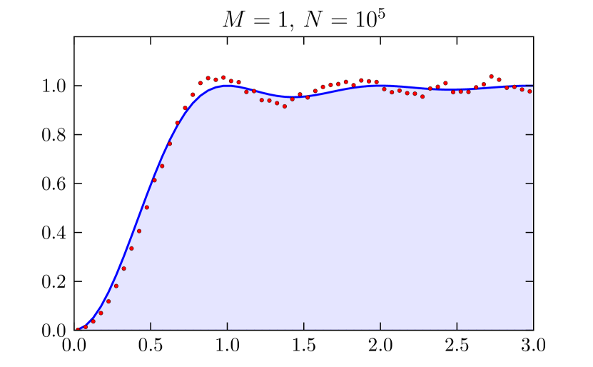
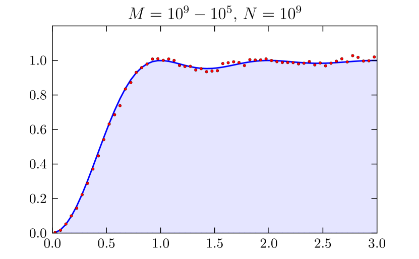
Figure 25: The solid line represents the RHS of (237) and the dots its LHS, computed from equation (131). The parameters are $\beta=\alpha+0.05$, $\alpha=(0,\,0.05,\,\dotsc,\,3)$ and the $x$-axis is given by $x=\tfrac{1}{2}\left(\alpha+\beta\right)$. Left: we use the first $10^{5}$ zeros. Right: the same parameters but using zeros in the middle of the critical line; $M=10^{9}-10^{5}$ and $N=10^{9}$.

Odlyzko’s conjecture (237) is a very strong constraint on the statistics of the zeros. Thus we submit the numerical solutions of equation (131), as discussed in the previous section, to this test. In Figure 25 (left) we can see the result for $M=1$ and $N=10^{5}$, with $\alpha$ ranging from $0\dotsc 3$ in steps of $s=0.05$, and $\beta=\alpha+s$ for each value of $\alpha$, i.e. $\alpha=(0.00,\,0.05,\,0.10,\dotsc,\,3.00)$ and $\beta=(0.05,\,0.10,\,\dotsc,\,3.05)$. We compute the left hand side of (237) for each pair $(\alpha,\beta)$ and plot the result against $x=\tfrac{1}{2}\left(\alpha+\beta\right)$. In Figure 25 (right) we do the same thing but with $M=10^{9}-10^{5}$ and $N=10^{9}$.

Clearly, the numerical solutions of (131) reproduce the correct statistics. In fact, Figure 25 (left) is identical to the one in Odlyzko2 . In Table 3 we provide the solutions to (131) at the end of the ranges considered, so that the reader may compare with Odlyzko ; Oliveira .

$n$	$y_{n}$
$10^{5}-5$	$74917.719415828$
$10^{5}-4$	$74918.370580227$
$10^{5}-3$	$74918.691433454$
$10^{5}-2$	$74919.075161121$
$10^{5}-1$	$74920.259793259$
$10^{5}$	$74920.827498994$

$n$	$y_{n}$
$10^{9}-5$	$371870202.244870467$
$10^{9}-4$	$371870202.673284457$
$10^{9}-3$	$371870203.177729799$
$10^{9}-2$	$371870203.274345928$
$10^{9}-1$	$371870203.802552324$
$10^{9}$	$371870203.837028053$

Table 3: Last numerical solutions to (131) around $n=10^{5}$ and $n=10^{9}$.

XV Prime number counting function revisited

In this section we explore whether our approximations to the Riemann zeros are accurate enough to reconstruct the prime number counting function. In Figure 26 (left) we plot $\pi(x)$ from equations (74) and (76), computed with the first $50$ zeros in the approximation $\rho_{n}=\tfrac{1}{2}+i\widetilde{y}_{n}$ given by (229). Figure 26 (right) shows the same plot with zeros obtained from the numerical solutions of equation (131). Although with the approximation $\widetilde{y}_{n}$ the curve is trying to follow the steps in $\pi(x)$, once again, one clearly sees the importance of the $\arg\zeta$ term.

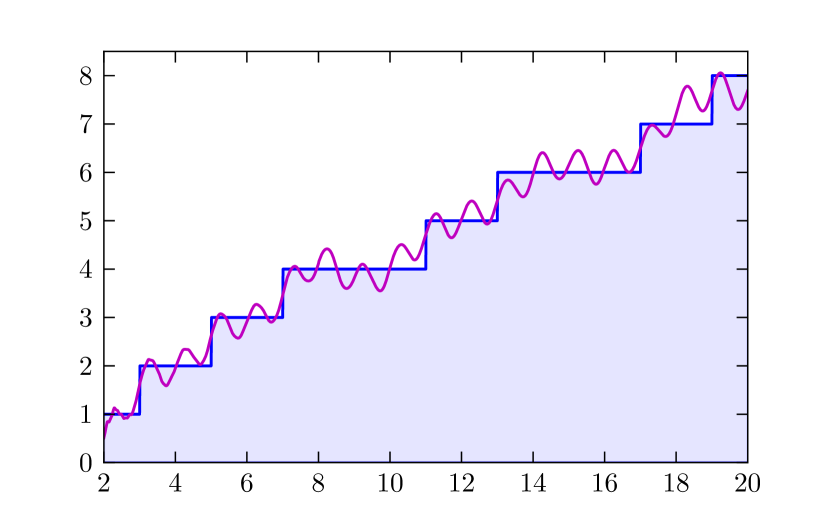
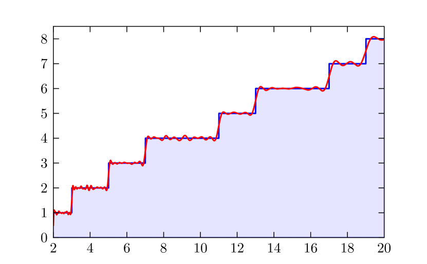
Figure 26: The prime number counting function $\pi(x)$ with the first $50$ Riemann zeros. Left: zeros approximated by the formula (229). Right: zeros obtained from numerical solutions to the equation (131).

XVI Solutions to the exact equation

In the previous sections we have computed numerical solutions of (131) showing that, actually, this first order approximation to (138) is very good and already captures some interesting properties of the Riemann zeros, like the GUE statistics and ability to reproduce the prime number counting formula. Nevertheless, by simply solving (138) it is possible to obtain values for the zeros as accurately as desirable. The numerical procedure is performed as follows:

1. We apply a root finder method on (138) looking for the solution in a region centered around the number $\widetilde{y}_{n}$ provided by (229), with a not so small $\delta$, for instance $\delta\sim 10^{-5}$.

2. We solve (138) again but now centered around the solution obtained in step 1 above, and we decrease $\delta$, for instance $\delta\sim 10^{-8}$.

3. We repeat the procedure in step 2 above, decreasing $\delta$ again.

4. Through successive iterations, and decreasing $\delta$ each time, it is possible to obtain solutions as accurate as desirable. In carrying this out, it is important to not allow $\delta$ to be exactly zero.

An actual implementation of the above procedure in Mathematica is shown in Appendix C. The first few zeros computed in this way are shown in Table 4. Through successive iterations it is possible achieve even much higher accuracy than these values.

$n$	$y_{n}$
$1$	$14.1347251417346937904572519835624702707842571156992431756855$
$2$	$21.0220396387715549926284795938969027773343405249027817546295$
$3$	$25.0108575801456887632137909925628218186595496725579966724965$
$4$	$30.4248761258595132103118975305840913201815600237154401809621$
$5$	$32.9350615877391896906623689640749034888127156035170390092800$

Table 4: The first few numerical solutions to (138), accurate to $60$ digits ($58$ decimals).

It is known that the first zero where Gram’s law fails is for $n=126$. Applying the same method, like for any other $n$, the solution of (138) starting with the approximation (229) does not present any difficulty. We easily found the following number:

$$y_{126}=279.229250927745189228409880451955359283492637405561293594727$$

Just to illustrate, and to convince the reader that the solutions of (138) can be made arbitrarily precise, we compute the zero $n=1000$ accurate up to $500$ decimal places, also using the same simple approach:

$$y_{1000}=1419. 42248094599568646598903807991681923210060106416601630469081468460$$

$$86764175930104179113432911792099874809842322605601187413974479526$$

$$50637067250834288983151845447688252593115944239425195484687708163$$

$$94625633238145779152841855934315118793290577642799801273605240944$$

$$61173370418189624947474596756904798398768401428049735900173547413$$

$$19116293486589463954542313208105699019807193917543029984881490193$$

$$19367182312642042727635891148784832999646735616085843651542517182$$

$$417956641495352443292193649483857772253460088$$

Substituting precise Riemann zeros into (138) one can check that the equation is identically satisfied. These results corroborate that (138) is an exact equation for the Riemann zeros.

XVII Numerical analysis: Dirichlet $L$-functions

We perform exactly the same numerical procedure as described in the previous section XVI, but now with equation (197) and (230) for Dirichlet $L$-functions.

We will illustrate our formulas with the primitive characters $\chi_{7,2}$ and $\chi_{7,3}$, since they possess the full generality of $a=0$ and $a=1$ and complex components. There are actually $\varphi(7)=6$ distinct characters mod $7$.

Example $\chi_{7,2}$.

Consider $k=7$ and $j=2$, i.e. we are computing the Dirichlet character $\chi_{7,2}(n)$. For this case $a=1$. Then we have the following components:

$$n$$

(238)

The first few zeros, positive and negative, obtained by solving (197) are shown in Table 5 (see Appendix C). The solutions shown are easily obtained with $50$ decimal places of accuracy, and agree with the ones in Oliveira2 , which were computed up to $20$ decimal places.

$n$	$\widetilde{y}_{n}$	$y_{n}$
$10$	$25.57$	$25.68439458577475868571703403827676455384372032540097$
$9$	$23.67$	$24.15466453997877089700472248737944003578203821931614$
$8$	$21.73$	$21.65252506979642618329545373529843196334089625358303$
$7$	$19.73$	$19.65122423323359536954110529158230382437142654926200$
$6$	$17.66$	$17.16141654370607042290552256158565828745960439000612$
$5$	$15.50$	$15.74686940763941532761353888536874657958310887967059$
$4$	$13.24$	$13.85454287448149778875634224346689375234567535103602$
$3$	$10.81$	$9.97989590209139315060581291354262017420478655402522$
$2$	$8.14$	$8.41361099147117759845752355454727442365106861800819$
$1$	$4.97$	$5.19811619946654558608428407430395403442607551643259$
$0$	$-3.44$	$-2.50937455292911971967838452268365746558148671924805$
$-1$	$-7.04$	$-7.48493173971596112913314844807905530366284046079242$
$-2$	$-9.85$	$-9.89354379409772210349418069925221744973779313289503$
$-3$	$-12.35$	$-12.25742488648921665489461478678500208978360618268664$
$-4$	$-14.67$	$-14.13507775903777080989456447454654848575048882728616$
$-5$	$-16.86$	$-17.71409256153115895322699037454043289926793578042465$
$-6$	$-18.96$	$-18.88909760017588073794865307957219593848843485334695$
$-7$	$-20.99$	$-20.60481911491253262583427068994945289180639925014034$
$-8$	$-22.95$	$-22.66635642792466587252079667063882618974425685038326$
$-9$	$-24.87$	$-25.28550752850252321309973718800386160807733038068585$

Table 5: Numerical solutions of (197) starting with the approximation (230), for the character (238). The solutions are accurate to $50$ decimal places and verified to $\left|L\left(\tfrac{1}{2}+iy_{n}\right)\right|\sim 10^{-50}$.

Example $\chi_{7,3}$.

Consider $k=7$ and $j=3$, such that $a=0$. In this case the components of $\chi_{7,3}(n)$ are the following:

$$n$$

(239)

The first few solutions of (197) are shown in Table 6 and are accurate up to $50$ decimal places, and agree with the ones obtained in Oliveira2 .

$n$	$\widetilde{y}_{n}$	$y_{n}$
$10$	$25.55$	$26.16994490801983565967242517629313321888238615283992$
$9$	$23.65$	$23.20367246134665537826174805893362248072979160004334$
$8$	$21.71$	$21.31464724410425595182027902594093075251557654412326$
$7$	$19.71$	$20.03055898508203028994206564551578139558919887432101$
$6$	$17.64$	$17.61605319887654241030080166645399190430725521508443$
$5$	$15.48$	$15.93744820468795955688957399890407546316342953223035$
$4$	$13.21$	$12.53254782268627400807230480038783642378927939761728$
$3$	$10.79$	$10.73611998749339311587424153504894305046993275660967$
$2$	$8.11$	$8.78555471449907536558015746317619235911936921514074$
$1$	$4.93$	$4.35640162473628422727957479051551913297149929441224$
$0$	$-5.45$	$-6.20123004275588129466099054628663166500168462793701$
$-1$	$-8.53$	$-7.92743089809203774838798659746549239024181788857305$
$-2$	$-11.15$	$-11.01044486207249042239362741094860371668883190429106$
$-3$	$-13.55$	$-13.82986789986136757061236809479729216775842888684529$
$-4$	$-15.80$	$-16.01372713415040781987211528577709085306698639304444$
$-5$	$-17.94$	$-18.04485754217402476822077016067233558476519398664936$
$-6$	$-20.00$	$-19.11388571948958246184820859785760690560580302023623$
$-7$	$-22.00$	$-22.75640595577430793123629559665860790727892846161121$
$-8$	$-23.94$	$-23.95593843516797851393076448042024914372113079309104$
$-9$	$-25.83$	$-25.72310440610835748550521669187512401719774475488087$

Table 6: Numerical solutions of (197) starting with the approximation (230), for the character (239). The solutions are accurate to $50$ decimal places and verified to $\left|L\left(\tfrac{1}{2}+iy_{n}\right)\right|\sim 10^{-50}$.

As stated previously, the solutions to equation (197) can be calculated to any desired level of accuracy. For instance, continuing with the character $\chi_{7,3}$, we can easily compute the following number for $n=1000$, accurate to $100$ decimal places, i.e. $104$ digits:

$$\begin{split}y_{1000}=1037.&56371706920654296560046127698168717112749601359549\\[-8.00003pt] &01734503731679747841764715443496546207885576444206\end{split}$$

We also have been able to solve the equation for high zeros to high accuracy, up to the millionth zero, some of which are listed in Table 7, and were previously unknown.

$n$	$\widetilde{y}_{n}$	$y_{n}$
$10^{3}$	$1037.61$	$1037.563717069206542965600461276981687171127496013595490$
$10^{4}$	$7787.18$	$7787.337916840954922060149425635486826208937584171726906$
$10^{5}$	$61951.04$	$61950.779420880674657842482173403370835983852937763461400$
$10^{6}$	$512684.78$	$512684.856698029779109684519709321053301710419463624401290$

Table 7: Higher zeros for the Dirichlet character (239). These solutions to (197) are accurate to $50$ decimal places.

XVIII Modular $L$-function based on Ramanujan $\tau$

In this section we study an $L$-function based on a level one modular form related to the Ramanujan $\tau$ function, and numerically solve the equations (216) and (232).

XVIII.1 Definition of the function

Here we will consider an example of a modular form of weight $k=12$. The simplest example is based on the Dedekind $\eta$-function

$$\eta(\tau)=q^{1/24}\,\prod_{n=1}^{\infty}(1-q^{n}).$$ (240)

Up to a simple factor, $\eta$ is the inverse of the chiral partition function of the free boson conformal field theory CFT , where $\tau$ is the modular parameter of the torus. The modular discriminant

$$\Delta(\tau)=\eta(\tau)^{24}=\sum_{n=1}^{\infty}\,\tau(n)\,q^{n}$$ (241)

is a weight $k=12$ modular form. It is closely related to the inverse of the partition function of the bosonic string in $26$ dimensions, where $24$ is the number of light-cone degrees of freedom StringTheo . The Fourier coefficients $\tau(n)$ correspond to the Ramanujan $\tau$-function, and the first few are

$$n$$

(242)

We then define the Dirichlet series

$$L_{\Delta}(z)=\sum_{n=1}^{\infty}\,\dfrac{\tau(n)}{n^{z}}.$$ (243)

Applying (216), the zeros are $\rho_{n}=6+iy_{n}$, where the $y_{n}$ satisfy the exact equation

$$\vartheta_{12}(y)+\lim_{\delta\to 0^{+}}\arg L_{\Delta}(6+\delta+iy_{n})=\left(n-\tfrac{1}{2}\right)\pi.$$ (244)

The counting function (218) and its asymptotic approximation are

$$N_{0}(T) =\dfrac{1}{\pi}\vartheta_{12}(T)+\dfrac{1}{\pi}\arg L_{\Delta}(6+iT)$$ (245)

$$\approx\dfrac{T}{\pi}\log\left(\dfrac{T}{2\pi e}\right)+\dfrac{1}{\pi}\arg L_{\Delta}(6+iT)+\dfrac{11}{4}.$$ (246)

A plot of (245) is shown in Figure 27, and we can see that it is a perfect staircase function.

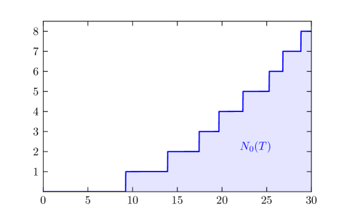
Figure 27: Exact counting formula (245) based on the Ramanujan $\tau$-function.

The approximate solution (232) now has the form

$$\widetilde{y}_{n}=\dfrac{\left(n-\tfrac{13}{4}\right)\pi}{W\left[(2e)^{-1}\left(n-\tfrac{13}{4}\right)\right]}$$ (247)

for $n=2,3,\dotsc$. Note that the above equation is valid for $n>1$, since $W(x)$ is not defined for $x<-1/e$.

XVIII.2 Numerical analysis

We follow exactly the same procedure, previously discussed in section XVI and implemented in Appendix C, to solve the equation (244) starting with the approximation provided by (247). Some of these solutions are shown in Table 8 and are accurate to $50$ decimal places.

$n$	$\widetilde{y}_{n}$	$y_{n}$
$1$		$9.22237939992110252224376719274347813552877062243201$
$2$	$12.46$	$13.90754986139213440644668132877021949175755235351449$
$3$	$16.27$	$17.44277697823447331355152513712726271870886652427527$
$4$	$19.30$	$19.65651314195496100012728175632130280161555091200324$
$5$	$21.94$	$22.33610363720986727568267445923624619245504695246527$
$6$	$24.35$	$25.27463654811236535674532419313346311859592673122941$
$7$	$26.60$	$26.80439115835040303257574923358456474715296800497933$
$8$	$28.72$	$28.83168262418687544502196191298438972569093668609124$
$9$	$30.74$	$31.17820949836025906449218889077405585464551198966267$
$10$	$32.68$	$32.77487538223120744183045567331198999909916163721260$
$100$	$143.03$	$143.08355526347845507373979776964664120256210342087127$
$200$	$235.55$	$235.74710143999213667703807130733621035921210614210694$
$300$	$318.61$	$318.36169446742310747533323741641236307865855919162340$

Table 8: Non-trivial zeros of the modular $L$-function based on the Ramanujan $\tau$-function, obtained from (244) starting with the approximation (247). These solutions are accurate to $50$ decimal places.

XIX Counterexample of Davenport-Heilbronn

The Davenport-Heilbronn function has almost all the same properties of $\zeta$, such as a functional equation, except that it has no Euler product formula. It is well known that such a function has zeros in the region $\Re\left(z\right)>1$ and zeros in the critical strip $0\leq\Re(z)\leq 1$, of which infinitely many of them lie on the critical line $\Re(z)=1/2$, but it also has zeros off of the critical line, thus violating the RH. Whether this is due to the absence of Euler product is unknown. It is very interesting to apply the formalism of the previous sections to this function and to understand clearly why the RH fails here. Such an exercise sharpens our understanding of the RH.

This function is somewhat contrived since it is linear combination of Dirichlet $L$-functions, designed to satisfy a functional equation. It is defined by

$${\cal D}(z)\equiv\dfrac{(1-i\kappa)}{2}L\left(z,\chi_{5,2}\right)+\dfrac{(1+i\kappa)}{2}L\left(z,\chi_{5,2}^{*}\right)$$ (248)

with

$$\kappa=\dfrac{\sqrt{10-2\sqrt{5}}-2}{\sqrt{5}-1},$$ (249)

and the Dirichlet character is given by

$$n$$

(250)

and $\chi_{5,2}(-1)=-1$ thus $a=1$. This function satisfies the functional equation

$$\xi(z)=\xi(1-z),\qquad\xi(z)\equiv\left(\dfrac{\pi}{5}\right)^{-z/2}\,\Gamma\left(\dfrac{1+z}{2}\right){\cal D}(z).$$ (251)

${\cal D}(z)$ has no Euler product because it is a linear combination of functions that do.

Now we repeat the analysis we presented for the Riemann $\zeta$-function. We have

$$\xi(z)=Ae^{i\theta},\qquad\xi(1-z)=A^{\prime}e^{-i\theta^{\prime}},$$ (252)

with $A(x,y)=A^{\prime}(x,y)$ and $\theta^{\prime}(x,y)=\theta(1-x,y)$, where

$$\theta(x,y)=\Im\left[\log\Gamma\left(\dfrac{1+x+iy}{2}\right)\right]-\dfrac{y}{2}\log\left(\dfrac{\pi}{5}\right)+\arg{\cal D}(x+iy).$$ (253)

As for previous $L$-functions, zeros should be characterized by our equation (149), namely

$$\theta+\theta^{\prime}=(2n+1)\pi.$$ (254)

The zeros on the critical line correspond to

$$\theta=\theta^{\prime}\quad\Rightarrow\quad\theta=\left(n+\tfrac{1}{2}\right)\pi.$$ (255)

As before, adopting the convention that the first positive zero is labeled by $n=1$, we shift $n\to n-1$, then the equation yielding zeros on the critical line is given by

$$\Xi(y_{n})+\lim_{\delta\to 0^{+}}\arg{\cal D}\left(\tfrac{1}{2}+\delta+iy_{n}\right)=\left(n-\tfrac{1}{2}\right)\pi$$ (256)

where

$$\Xi(y)\equiv\Im\left[\log\Gamma\left(\dfrac{3}{4}+i\dfrac{y}{2}\right)\right]-\dfrac{y}{2}\log\left(\dfrac{\pi}{5}\right).$$ (257)

Expanding $\Gamma(z)$ through Stirling’s formula and neglecting the $\arg{\cal D}$ term in (256) it is possible to obtain an explicit approximate solution given by

$$\widetilde{y}_{n}=\dfrac{2\pi\left(n-\tfrac{5}{8}\right)}{W\left[5e^{-1}(n-\tfrac{5}{8})\right]},$$ (258)

where $n=1,2,\dotsc$ and $W$ denotes the principal branch $W_{0}$ of the Lambert function (220).

Now we can numerically solve (256) starting with the approximation given by (258). The first few solutions are shown in Table 9 (left).

$n$	$\widetilde{y}_{n}$	$y_{n}$
$1$	$5.32$	$5.094159844584467267$
$2$	$8.96$	$8.939914408100472858$
$3$	$11.93$	$12.133545425790163309$
$4$	$14.60$	$14.404003112292645158$
$5$	$17.08$	$17.130239400567288918$
$6$	$19.43$	$19.308800174241700381$
$7$	$21.68$	$22.159707765035018919$
$8$	$23.85$	$23.345370112090190151$
$9$	$25.95$	$26.094967346227912542$
$10$	$28.00$	$27.923798821611878096$

$\rho$	$\tfrac{1}{\pi}\theta$	$\tfrac{1}{\pi}(\theta+\theta^{\prime})$
$0.8085171825+i\,85.6993484854$	$44.092$	$89$
$0.6508300806+i\,114.1633427308$	$64.026$	$127$
$0.5743560504+i\,166.4793059132$	$103.023$	$207$
$0.7242576946+i\,176.7024612429$	$111.075$	$223$
$0.8695305796+i\,240.4046723514$	$163.055$	$325$
$0.8195495921+i\,320.8764896688$	$232.106$	$465$
$0.7682231236+i\,331.0502594079$	$241.098$	$483$
$0.6285081083+i\,366.6409075762$	$273.027$	$545$
$0.8158736778+i\,411.7967375490$	$314.133$	$629$
$0.7088822242+i\,440.4845107397$	$341.017$	$681$

Table 9: Left: first few zeros of (248) on the critical line, $\rho_{n}=\tfrac{1}{2}+iy_{n}$, computed from (256) starting with the approximation (258). Right: We can see that equation (254) is indeed verified for the first few zeros off of the critical line. Note that $\tfrac{1}{\pi}\theta$ can be any real number, while the combination $\tfrac{1}{\pi}\left(\theta+\theta^{\prime}\right)$ always gives an odd integer at a non-trivial zero.

As for the trivial zeros of $\zeta$ we expect that zeros off of the line also satisfy (254). We indeed verified this. It is more difficult to find these zeros since they are at scattered values of $x$, but it is in fact feasible. In Table 9 (right) we show some of the lower zeros and the values of $\tfrac{1}{\pi}(\theta+\theta^{\prime})$, which are odd integers. In Figure 28 we show the contour lines of (251), i.e. $\xi(z)=u(x,y)+iv(x,y)$, and we consider the lines $u=0$ and $v=0$. On the critical line $x=1/2$ we have a $v=0$ contour everywhere, and we approach the zero on a $u=0$ contour through the $\delta$ limit, as shown in equation (256). In this case the $\delta$ smooths out the discontinuity. However, note how the curves $u=0$ are very different in nature for zeros off of the critical line. In this case the $\delta$ limit does not smooth out the function, since the path to approach the zero is more involved. Nevertheless, equation (254) is still satisfied for these zeros off of the critical line.

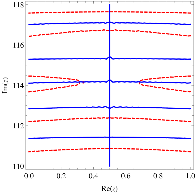
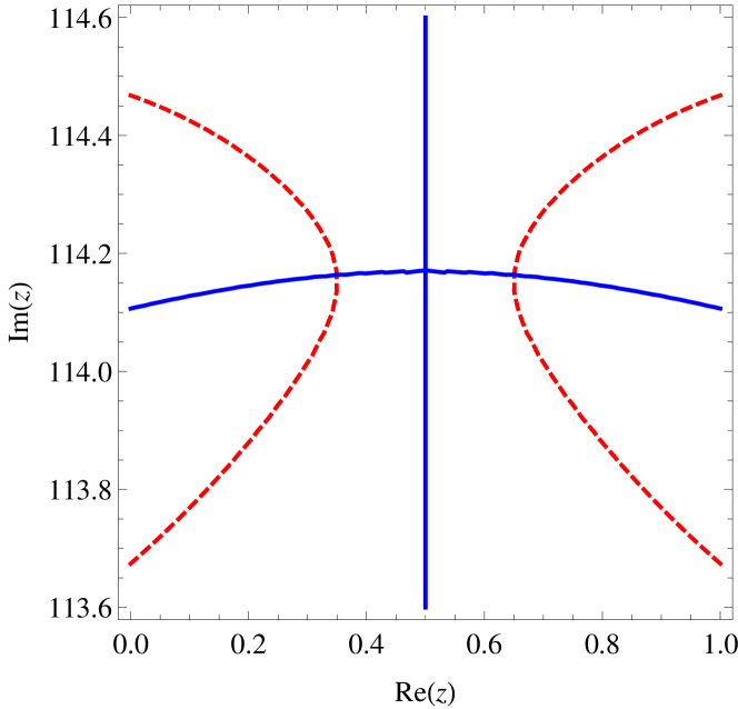
Figure 28: Contour plot of $\xi=u+iv$, equation (251), for $x=0\dotsc 1$ and $y=110\dotsc 118$. Note the zeros off-line for $y\approx 114.1633$. The solid (blue) lines correspond to curves $v=0$ and the dashed (red) lines to $u=0$.

If there is a unique solution to (256) for every $n$, then as for the $\zeta$-function we can determine $N_{0}(T)$ which counts zeros on the line. However, the equation (256) is not defined for every $n$. For instance, for $n=44$ and $n=45$ this equation has no solution, as illustrated in Figure 29. The same thing happens again for $n=64$ and $n=65$, for $n=103$ and $n=104$, and so on.

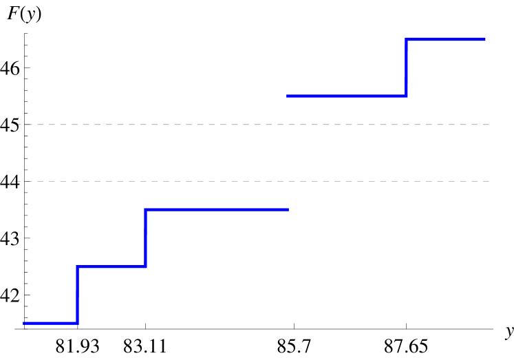
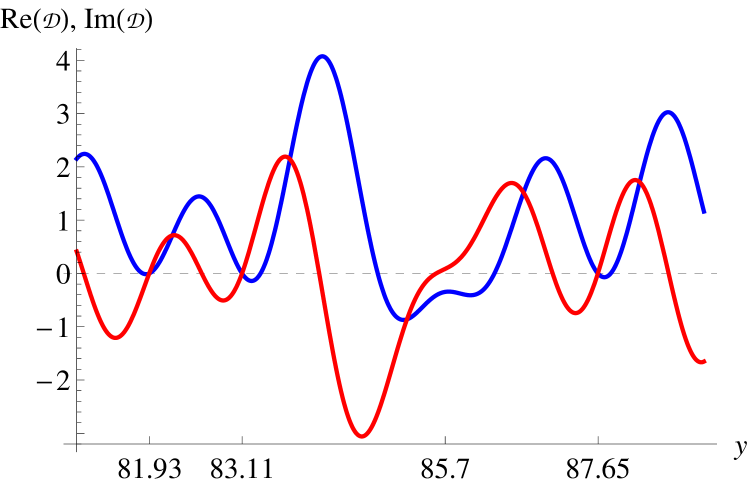
Figure 29: Left: $F(y)=\tfrac{1}{\pi}\left(\Xi(y)+\arg{\cal D}\left(\tfrac{1}{2}+\delta+iy\right)\right)+\tfrac{1}{2}$ versus $y$. Note the discontinuity in the graph for $y\approx 85.6993$, corresponding to $n=44$ and $n=45$, where the equation (256) has no solution. Right: the blue line is $\Re\left({\cal D}\left(\tfrac{1}{2}+iy\right)\right)$ and the red line is $\Im\left({\cal D}\left(\tfrac{1}{2}+iy\right)\right)$. Equation (256) is not defined since $\arg{\cal D}\left(\tfrac{1}{2}+iy\right)$ changes branch. Note that $\Re({\cal D})<0$ and $\Im({\cal D})=0$ at $y\approx 85.6993$, where there are two zeros off the line at this height.

If $N(T)$ counts zeros on the entire strip, then clearly $N_{0}(T)\neq N(T)$. For these values of $y$, corresponding to zeros off the line, $\lim_{\delta\to 0^{+}}\arg{\cal D}\left(\tfrac{1}{2}+\delta+iy\right)$ is not defined, i.e. the $\delta$ limit does not smooth out the function since there is a severe change of branch. This is why the equation (256) is not defined in the vicinity of such $y$’s. In Figure 30 (left) we show a plot of $\tfrac{1}{\pi}\left[\theta(x+\delta,y)+\theta^{\prime}(x+\delta,y)\right]$ for $x=0\dotsc 1$ and $y=81\dotsc 90$. Note that there are zeros off the line at $y\approx 85.6993$. We included a $\delta\sim 10^{-1}$. Note how the function can be smoothed on the critical line $x=1/2$ if there are only zeros on the line. However, when there are zeros off of the critical line the function cannot be made continuous (note the “big hole” around the critical line).

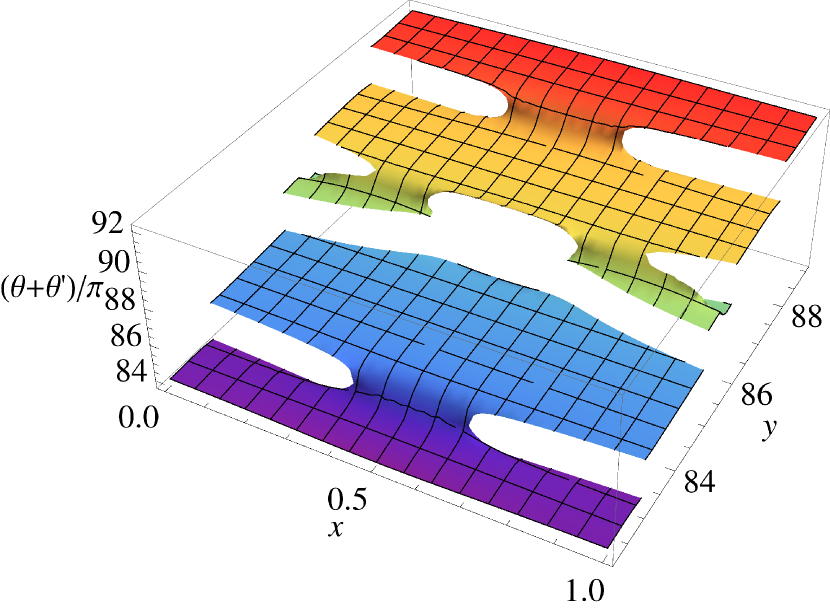
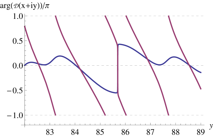
Figure 30: Left: The zeros off-line do not allow the function to be smoothed on the critical line. Right: the blue line is $\tfrac{1}{\pi}\arg{\cal D}(x+iy)/\pi$ versus $y$, in the vicinity of the first zero off the line, where $x\approx 0.8085$. The purple line is $\tfrac{1}{\pi}\arg{\cal D}(1-x+iy)$.

Finally, in Figure 30 (right) we plot the analog of Figure 14 (right). In the vicinity of the first zero off of the critical line, both $\theta$ and $\theta^{\prime}$ are well-defined and there is a solution to (254).

For Riemann $\zeta$, we provided arguments that there is a unique solution to the analogous equation (138), implying that $N_{0}(T)=N(T)$. If $\arg\zeta\left(\tfrac{1}{2}+iy\right)$ does not change branch, or if it changes “very little”, the $\delta$ limit smooths out the function bringing it to the principal branch, making the equation well defined. On the other hand, if there is a severe change of branch it is impossible to make this function continuous, which is the case here for the function (248) (see Figures 29 and 30).

The important difference with $\zeta$ is that

$$S_{\cal D}(y)=\lim_{\delta\to 0^{+}}\dfrac{1}{\pi}\arg{\cal D}\left(\tfrac{1}{2}+\delta+y\right)$$ (259)

has very different properties in comparison to $S(y)=\lim_{\delta\to 0^{+}}\tfrac{1}{\pi}\arg\zeta\left(\tfrac{1}{2}+\delta+iy\right)$ or the argument of the other $L$-functions we have considered. The properties conjectured for $S(y)$ in section VIII should not hold. The repeated changes in branch indicate that $S_{\cal D}(y)$ has the behavior shown in Figure 31.

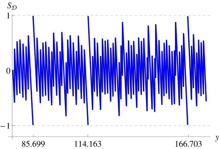
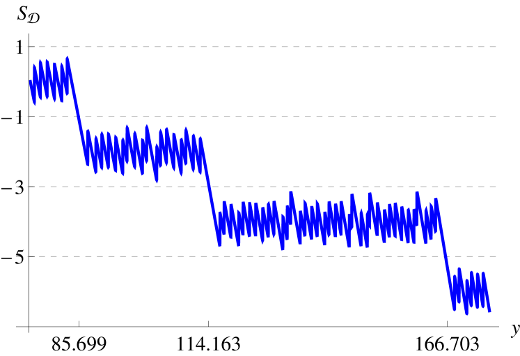
Figure 31: Left: $S_{{\cal D}}$ in the principal branch. Right: $S_{{\cal D}}$ explicitly showing the changes in branch. Clearly $\langle S_{{\cal D}}\rangle\neq 0$. We also have $|S_{{\cal D}}|\gg C\log y$, contrary to $|S(y)|<C\log y$ for $\zeta$.

In particular, the average

$$\langle S_{\cal D}(y)\rangle\neq 0$$ (260)

in clear contrast to $\zeta$ where the average has been proven to be zero. The points on the $y$-axis shown in Figure 31 correspond to zeros off of the critical line. For these zeros $S_{{\cal D}}(y)$ jumps by $2$, passing to another branch without coming back to the principal branch. This is a very different behaviour in comparison to the picture described for $\zeta$ in Section VIII (see Figures 16 and 17).

XX Saddle point approximation

The original aim of the work in this section was to obtain an approximate analytic expression for $\arg\zeta(\tfrac{1}{2}+iy)$ because of its importance to the whole theory of the zeros. For the smooth part, $\arg\Gamma$, one has such an expression due to the Stirling’s approximation, and we will present something similar for $\zeta$.

The saddle-point method, also known as steepest descent method, approximates integrals of the type

$$I(\lambda)=\int_{{\cal C}}e^{\lambda f(u)}du$$ (261)

for large $\lambda$. The saddle-points are solutions to $f^{\prime}(u)=0$, provided $f^{\prime\prime}(u)\neq 0$, where $f^{\prime}$ and $f^{\prime\prime}$ are the first and second derivatives of $f$. For simplicity let us consider only one saddle point denoted by $s$. The contour ${\cal C}$ must be deformed in such a way as to pass through $u=s$ with $\Re(u)$ having the steepest descent (hence the name). If $f(u)$ is an analytic function, using $f(u)\approx f(s)+\tfrac{1}{2}f^{\prime\prime}(s)(u-s)^{2}$ one is left with a gaussian integral and obtains

$$I(\lambda)\approx\sqrt{\dfrac{2\pi}{-f^{\prime\prime}\left(s\right)}}\ e^{\lambda f(s)}.$$ (262)

Let us consider a very illustrative example, the result of which we will need later. The $\Gamma$-function has the integral representation

$$\Gamma(z)=\int_{0}^{\infty}u^{z-1}e^{-u}du,\qquad\Re(z)>0.$$ (263)

Writing the integrand as $e^{f(u)}$ where $f(u)=-u+(z-1)\log u$, then $f^{\prime}(u)=0$ implies $s=z-1$. Then (262) yields

$$\Gamma(z)\approx\sqrt{2\pi}(z-1)^{z-1/2}\,e^{-(z-1)}.$$ (264)

For $n$ a positive integer, $\Gamma(n+1)=n!\approx\sqrt{2\pi}\,n^{n+1/2}\,e^{-n}$, which is the very useful Stirling’s approximation. Since the above approximation is an analytic function of $z$, it is valid in the whole complex plane through analytic continuation. It is very useful for instance to determine the asymptotic expansion of the Riemann-Siegel $\vartheta$ function,

$$\vartheta(y)=\arg\Gamma\left(\tfrac{1}{4}+\tfrac{iy}{2}\right)-y\log\sqrt{\pi}\approx\dfrac{y}{2}\log\left(\dfrac{y}{2\pi e}\right)-\dfrac{\pi}{8}$$ (265)

where as usual $\arg\Gamma=\Im\log\Gamma$.

Now let us consider the $\zeta$-function, which has the well known integral representation

$$\zeta(z)=\dfrac{1}{\Gamma(z)}\int_{0}^{\infty}\dfrac{u^{z-1}}{e^{u}-1}\,du,\qquad\Re(z)>1.$$ (266)

If $z\gg 1$ is real, then the saddle point of the integrand in (266) is far from the origin, and one can approximate $e^{u}-1\approx e^{u}$, then this integral is approximately the same as (263), showing that for real $z$ then $\zeta(z)\to 1$ as $z\to\infty$. The above integral is badly behaved at the origin $u=0$, thus let us introduce a small parameter $\mu$, having in mind that we can always take the limit $\mu\to 0^{+}$. The above integral arises in quantum statistical physics, and $\mu$ is minus the chemical potential. Thus we introduce

$$\zeta(z)=\lim_{\mu\to 0^{+}}\,\dfrac{1}{\Gamma(z)}\int_{0}^{\infty}\dfrac{u^{z-1}}{e^{u+\mu}-1}\,du.$$ (267)

We want to estimate this integral through the saddle-point method. For this aim we can write the integrand in the form $e^{f(u)}$ where

$$f(u)=(z-1)\log u-\log\left(e^{u+\mu}-1\right).$$ (268)

The condition $f^{\prime}(u)=0$ yields the transcendental equation

$$\dfrac{z-1}{u}=\dfrac{e^{u+\mu}}{e^{u+\mu}-1},$$ (269)

which can be solved explicitly, determining the saddle points in the following form:

$$s_{k}(z)=z-1+w_{k}(z),$$ (270)

with

$$w_{k}(z)=W_{k}\left[(1-z)e^{1-z-\mu}\right],$$

where $W_{k}$ is the $k$-th branch of the multi-valued Lambert $W$ function (220). Note that setting $w_{k}=0$, one recovers the saddle point for the $\Gamma$-function.

One can easily show that

$$f(s_{k})=-s_{k}-\mu+(z-2)\log s_{k}+\log(z-1)$$ (271)

and

$$f^{\prime\prime}(s_{k})=\dfrac{(1+w_{k})}{(1-z)\left(1+\tfrac{w_{k}}{z-1}\right)^{2}}.$$ (272)

For real $z$ (270) yields only one saddle-point given by the principal branch $k=0$. For complex $z$ we have an infinite number of saddle-points. However, not all of them contribute to the integral (267), since according to the integration path we must choose the ones which satisfy $\Re(s_{k})>0$. Using equations (271), (272) and dividing by the Stirling approximation to $\Gamma(z)$, equation (264), one then obtains

$$\zeta(z)\approx\sum_{k}{}^{{}^{\prime}}\zeta_{k}(z)$$ (273)

where

$$\zeta_{k}(z)=\exp\left\{(z-1)\log\left(1+\dfrac{w_{k}}{(z-1)}\right)-w_{k}-\mu-\dfrac{1}{2}\log\left(w_{k}+1\right)\right\}.$$ (274)

In the above formula (273) the $\mu\to 0^{+}$ is implicit. The sum over integers $k$ must be taken according to the condition $\Re(s_{k})>0$.

In obtaining (273) it is important to note that (268) is not an analytic function, since $\log u$ has branches for $u\in\mathbb{C}$. Thus we are taking into account the contribution of each different branch $k$ for the saddle-points. This goes a little beyond the assumptions of the saddle-point method (262).

For real values of $z$ there is only one saddle-point corresponding to $k=0$ in (273). This approximation describes the $\zeta(z)$ very well over this range, as shown in Figure 32 (left).

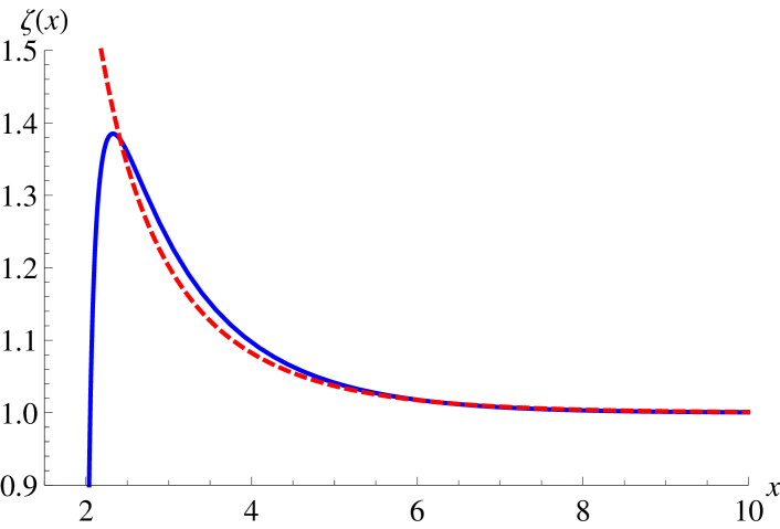
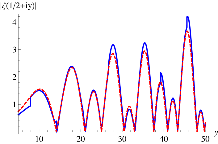
Figure 32: The dashed (red) line corresponds to the exact $\zeta(z)$ while the solid (blue) line corresponds to the saddle point approximation (273). Left: real values. Right: complex values on the critical line.

For complex values in the approximation (273) we need to consider the contribution for different branches $k$. On the critical line $z=1/2+iy$, a plot of the absolute value of (273) is shown in Figure 32 (right). The number of saddle points varies with $y$. For instance, for $y\sim 15$ we need $k=-2,-1,0$ and for $y\sim 30$ we need $k=-4,-3,\dotsc,0$. Thus the sum in (273) ranges differently for each value of $y$.

Roughly, the number of branches one needs is $-|y|/2\pi<k\leq 0$ which can be obtained from the condition $\Re(s_{k})>0$ (the branches $k>0$ can be neglected). This approximation works surprisingly well, as Figure 32 shows; it clearly captures the zeros. However it remains difficult to characterize $\arg\zeta$ precisely, because of the sum over branches $k$.

XXI Discussion and open problems

In the second half of these lectures we have provided new insights into the RH. We have actually proposed several concrete strategies towards its proof which are all based on analysis. Let us list some of the main open problems, namely what is needed to complete this program.

1. Is there a more rigorous derivation of our main equation (149), i.e. $\theta+\theta^{\prime}=(2n+1)\pi$? It is a powerful new equation that is valid whether the RH is true or not and contains detailed information about the zeros since they enumerated by the integer $n$. It is evidently correct and captures all zeros, trivial or non-trivial, of the multitude of functions considered in this paper, including functions with zeros off of the critical line, where the RH fails. This seems to be a matter of carefully defining the limit as one approaches a zero.

2. Can one prove there is a unique solution to the transcendental equation (138) for every $n$? As explained, this would imply the RH is true since then $N_{0}(T)=N(T)$. We provided arguments that the $\delta\to 0^{+}$ prescription smooths out the function $S(y)$ sufficiently so that there is indeed a unique solution. We also showed that it is precisely this property that fails for the Davenport-Heilbronn function, where the RH is false.

3. We proposed that $S(y)$ is nearly always on the principal branch and thus $S(y)=O(1)$ which is much smaller than $O(\log y)$. Can this be rigorously proven? Actually this is not necessary for proving the RH along the lines described here, but rather would be a consequence. We conjectured that the bounce number $b$, which is the average of $|S(y)|$ on the zeros, defined in equation (169), is in the range $1/4<b<1/2$.

4. Can one prove that the real electric potential $\Phi(x,y)$ is a regular alternating function along the line $\Re(z)=1$? We showed this asymptotically, but only in a crude approximation. We argued that this would also establish the RH. Can the latter be proven?

5. Can one prove directly that there are no zeros off of the critical line by proving there are no solutions to $\theta(x,y)+\theta^{\prime}(x,y)=(2n+1)\pi$ for $x\neq 1/2$? We suggested one approach, based on the observation that the left hand side of this equation has very little dependence on $x$ for $x>1/2$ (see Figure 13). Since we know there are no solutions for $x\geq 1$, i.e. there are no zeros with $x\geq 1$, this suggests that this would imply there are no zeros for $x>1/2$, since the curve for $x>1/2$ is essentially the same as at $x=1$, and there we know there are no solutions. Can this argument be made more precise? This is an appealing idea since the RH would then be related to the fact that there are no zeros with $x\geq 1$, which follows from the Euler product formula. Functions such as the Davenport-Heilbronn function where the RH fails do not have an Euler product formula.

Appendix A The Perron formula

Consider the sum

$$A(x)=\sum_{n\leq x}{}^{{}^{\prime}}a(n)$$ (275)

where $a(n)$ is an arithmetic function. Here, the prime on the summation indicates that the last term of the sum must be multiplied by $1/2$ when $x$ is an integer. One has the following integral:

$$\int_{0}^{\infty}A(x)x^{-z-1}dx=\int_{0}^{\infty}\left(\sum_{n\leq x}a(n)\right)x^{-z-1}dx=-\dfrac{1}{z}\int_{0}^{\infty}\left(\sum_{n\leq x}a(n)\right)\dfrac{d}{dx}\left(x^{-z}\right)dx.$$ (276)

Since $A(x)$ is a sequence of step functions, and the derivative of a step function is the Dirac delta-function, one has

$$\dfrac{d}{dx}\sum_{n\leq x}a(n)=a(n)\delta(x-n)$$

Integrating the above expression by parts one obtains

$$\dfrac{g(z)}{z}=\int_{0}^{\infty}A(x)x^{-z-1}dx.$$ (277)

where

$$g(z)=\sum_{n=1}^{\infty}\dfrac{a(n)}{n^{z}}.$$ (278)

The standard definition of the Mellin transform ${\cal M}f$ of the function $f$ is

$$({\cal M}f)(s)=\varphi(s)=\int_{0}^{\infty}x^{s-1}f(x)dx.$$ (279)

Its inverse is well-known:

$$({\cal M}^{-1}\varphi)(x)=f(x)=\dfrac{1}{2\pi i}\int_{c-i\infty}^{c+i\infty}x^{-s}\varphi(s)ds.$$ (280)

Identifying $s=-z$, $\varphi(-z)=g(z)/z$, and $f(x)=A(x)$ one obtains (84).

Appendix B Counting formula on the entire critical strip

The argument principle enables us to count zeros and poles of a complex function inside a simply connected bounded region. Let us consider two functions $f(z)$ and $g(z)$, such that $f$ is analytic and $g$ is meromorphic inside and on a given closed contour ${\cal C}$. Thus we can write

$$g(z)=(z-w_{1})^{n_{1}}(z-w_{2})^{n_{2}}\dotsm\dfrac{1}{(z-\overline{w}_{1})^{\overline{n}_{1}}(z-\overline{w}_{2})^{\overline{n}_{2}}\dotsm}\,h(z)$$ (281)

where $w_{i}$ and $\overline{w}_{i}$ denotes the zeros and poles, respectively, with its respective multiplicities $n_{i}$ and order $\overline{n}_{i}$, and $h(z)$ is analytic and without zeros or poles in and on ${\cal C}$. Then we have

$$\dfrac{g^{\prime}(z)}{g(z)}=\dfrac{d}{dz}\log g(z)=\dfrac{n_{1}}{z-w_{1}}+\dfrac{n_{2}}{z-w_{2}}+\dotsm-\dfrac{\overline{n}_{1}}{z-\overline{w}_{1}}-\dfrac{\overline{n}_{2}}{z-\overline{w}_{2}}-\dotsm+\dfrac{h^{\prime}(z)}{h(z)}.$$ (282)

Assuming that $g(z)$ has no zeros or poles on the contour ${\cal C}$, we thus have

$$\oint_{{\cal C}}f(z)\dfrac{g^{\prime}(z)}{g(z)}dz=\sum_{i}n_{i}\oint_{{\cal C}}\dfrac{f(z)}{z-w_{i}}dz-\sum_{j}\overline{n}_{j}\oint_{{\cal C}}\dfrac{f(z)}{z-\overline{w}_{j}}dz+\oint_{{\cal C}}f(z)\dfrac{h^{\prime}(z)}{h(z)}dz.$$ (283)

Since $\tfrac{fh^{\prime}}{h}$ is analytic, the last integral vanishes by Cauchy’s integral theorem. By Cauchy’s integral formula we therefore have

$$\dfrac{1}{2\pi i}\oint_{{\cal C}}f(z)\dfrac{g^{\prime}(z)}{g(z)}dz=\sum_{i}n_{i}f(w_{i})-\sum_{j}\overline{n}_{j}f(\overline{w}_{j}).$$ (284)

Now setting $f(z)=1$ we have Cauchy’s argument principle

$$\dfrac{1}{2\pi i}\oint_{{\cal C}}\dfrac{g^{\prime}(z)}{g(z)}dz=N-\overline{N},$$ (285)

where $N=\sum_{i}n_{i}$ is the number of zeros inside ${\cal C}$, including multiplicities, and $\overline{N}=\sum_{j}\overline{n}_{j}$ is the number of poles, accounting its orders.

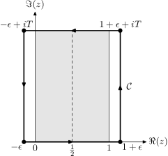
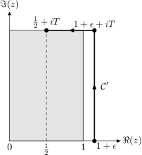
Figure 33: Left: contour ${\cal C}$ for (287) in the counterclockwise direction. The contour must have no zeros on it. The critical line $\Re(z)=1/2$ splits the rectangle in half. Right: it is equivalent to consider the contour ${\cal C}^{\prime}$.

Now let us use (285) to count the zeros of $\zeta(z)$ inside the region $0\leq\Re(z)\leq 1$ and $0\leq\Im(z)\leq T$. Remember that $\zeta(z)$ and $\chi(z)$ have the same zeros in this region. Since $\zeta(z)$ has a simple pole at $z=1$, and so has $\chi(z)$, we consider the function

$$\xi(z)\equiv\tfrac{1}{2}z(z-1)\pi^{-z/2}\,\Gamma\left(z/2\right)\zeta(z),$$ (286)

which is entire and has no poles. Note that $\zeta(z)$, and thus $\xi(z)$, has no zeros along the positive real line, and according to (285) we must assume that $T$ does not correspond to the imaginary part of a zero. Then from (285) we have

$$N(T)=\dfrac{1}{2\pi}\Im\left[\oint_{{\cal C}}\dfrac{\xi^{\prime}(z)}{\xi(z)}dz\right],$$ (287)

where the contour ${\cal C}$ is chosen to be the boundary of the rectangle with vertices at the points $z\in\left\{-\epsilon,\,1+\epsilon,\,1+\epsilon+iT,\,-\epsilon+iT\right\}$, as illustrated in Figure 33 (left). Since $\xi(z)$ is real on the real line, the integration along the line segment $[-\epsilon,1+\epsilon]$ does not contribute to (287). Moreover, since $\xi(z)=\xi(1-z)$ we can consider just the right half of the rectangle, whose contribution to the integral (287) comes from line segments $[1+\epsilon,1+\epsilon+iT]$ and $[1+\epsilon+iT,1/2+iT]$. This is the contour ${\cal C}^{\prime}$ shown in Figure 33 (right). Therefore we have

$$N(T) =\dfrac{1}{\pi}\Im\int_{{\cal C}^{\prime}}dz\,\dfrac{d}{dz}\log\xi(z)$$ (288)

$$=\dfrac{1}{\pi}\Im\int_{{\cal C}^{\prime}}dz\,\dfrac{d}{dz}\left[\log\left(\tfrac{1}{2}z(z-1)\right)+\log\left(\pi^{-z/2}\Gamma\left(z/2\right)\right)+\log\zeta(z)\right].$$ (289)

The first term in (289) gives

$$\dfrac{1}{\pi}\Im\left.\log\left[\tfrac{1}{2}z(z-1)\right]\right|_{1+\epsilon}^{1/2+iT}=\dfrac{1}{\pi}\Im\log\left(-\tfrac{1}{2}\left(T^{2}+\tfrac{1}{4}\right)\right)=1.$$ (290)

For the second term in (289), since $\pi^{-z/2}\Gamma(z/2)$ is analytic and real on $z=1+\epsilon$, we have the contribution only from the end point of the contour, which gives

$$\dfrac{1}{\pi}\Im\log\Gamma\left(\tfrac{1}{4}+i\tfrac{T}{2}\right)-\dfrac{T}{2\pi}\log\pi\equiv\dfrac{1}{\pi}\vartheta\left(T\right),$$ (291)

where we have the Riemann-Siegel $\vartheta$ function. Therefore, the number of zeros in the critical strip up to height $T$ is given by

$$N(T)=\dfrac{1}{\pi}\vartheta(T)+1+S(T)$$ (292)

where

$$S(T)\equiv\dfrac{1}{\pi}\Im\int_{{\cal C}^{\prime}}d\left(\log\zeta(z)\right)=\dfrac{1}{\pi}\Delta_{{\cal C}^{\prime}}\arg\zeta(z).$$ (293)

The above formula (292) is known as the Backlund counting formula. Note that $\Im\log\zeta=\arg\zeta$. The above result consists in computing the variation of $\arg\zeta(z)$ through the line segments starting at $z=1+\epsilon$, where $\arg\zeta(1+\epsilon)=0$, then up to $z=1+\epsilon+iT$, then finally to $z=1/2+iT$. Since the integrand in (293) is a total derivative, it is tempting to write $S(T)=\tfrac{1}{\pi}\Im\log\zeta\left(1/2+iT\right)=\tfrac{1}{\pi}\arg\zeta(1/2+iT)$, corresponding to the end point of the contour ${\cal C}^{\prime}$. However, this must be carefully considered since $\log\zeta(z)$ can not be always in the principal branch along ${\cal C}^{\prime}$. Nevertheless, if $\Re\left(\zeta\right)>0$ for all $z$ on ${\cal C}^{\prime}$, then $\log\zeta(z)$ is well defined and is always in the principal branch, i.e. $\log\zeta(z)=\log|\zeta(z)|+i\arg\zeta(z)$ with $-\pi/2<\arg\zeta(z)\leq\pi/2$. In such a case it is valid to set $S(T)=\tfrac{1}{\pi}\arg\zeta(1/2+iT)$, and we also have $|S(T)|<1/2$.

Let us now consider $z=x+iy$ for $x\geq 2$. From the series $\zeta(z)=\sum_{n=1}^{\infty}n^{-z}$ we have

$$\Re\left(\zeta\right)=1+\dfrac{\cos\left(y\log 2\right)}{2^{x}}+\dfrac{\cos\left(y\log 3\right)}{3^{x}}+\dotsm\geq 1-\left(\dfrac{1}{2^{x}}+\dfrac{1}{3^{x}}+\dotsm\right).$$ (294)

Since $x\geq 2$ we also have

$$\dfrac{1}{2^{x}}+\dfrac{1}{3^{x}}+\dfrac{1}{4^{x}}+\dotsm\leq\dfrac{1}{2^{2}}+\dfrac{1}{3^{2}}+\dfrac{1}{4^{2}}+\dotsm=\zeta(2)-1=\dfrac{\pi^{2}}{6}-1$$ (295)

Therefore

$$\Re\left(\zeta\right)>\dfrac{12-\pi^{2}}{6}>0.$$ (296)

For this reason it is often assumed $\epsilon=1$ in the contour ${\cal C}^{\prime}$ appearing in (293). In this way one only needs to analyze the behaviour of $\Re\left(\zeta\right)$ along the horizontal line joining the points $2+iT$ and $\tfrac{1}{2}+iT$.

If one expands $\Gamma(z)$ in (291) through Stirling’s formula one obtains

$$\vartheta(T)=\dfrac{T}{2}\log\left(\dfrac{T}{2\pi e}\right)-\dfrac{\pi}{8}+O\left(T^{-1}\right).$$ (297)

Then (292) yields the Riemann-von Mangoldt counting formula

$$N(T)=\dfrac{T}{2\pi}\log\left(\dfrac{T}{2\pi}\right)-\dfrac{T}{2\pi}+\dfrac{7}{8}+S(T)+O\left(T^{-1}\right).$$ (298)

Appendix C Mathematica code

Here we provide a simple Mathematica implementation to compute the zeros of $L$-functions based on the previous transcendental equations. We will consider Dirichlet $L$-functions, since it involves more ingredients, like the modulus $k$, the order $a$ and the Gauss sum $G(\tau)$. For the Riemann $\zeta$-function the procedure is trivially adapted, as well as for the Ramanujan $\tau$-function of section XVIII.

The function (195) is implemented as follows:

⬇

RSTheta[y_, a_, k_] := Im[LogGamma[1/4 + a/2 + I*y/2]] - y/2*Log[Pi/k]

For the transcendental equation (197) we have

⬇

ExactEq[n_, y_, s_, a_, k_, j_, G_, n0_] :=

(RSTheta[y, a, k] + Arg[DirichletL[k, j, 1/2 + s + I*y]] -1/2*Arg[G])/Pi + a/4 + 1/2 - n + n0

Above, s denotes $0<\delta\ll 1$, a is the order (177), k is the modulus, j specify the Dirichlet character $\chi_{k,j}$ (as discussed in section IX), and G is the Gauss sum (173). Note that we also included n0, discussed after (196), but we always set $n_{0}=0$ for the cases analysed in section XVII. The implementation of the approximate solution (230) is

⬇

Sgn[n_] := Which[n != 0, Sign[n], n == 0, -1]

A[n_, a_, G_, n0_] := Sgn[n]*(n - n0 + 1/2/Pi*Arg[G]) + (1 - 4*Sgn[n] - 2*a*(Sgn[n] + 1))/8

yApprox[n_, a_, G_, k_, n0_] := 2*Pi*Sgn[n]*A[n, a, G, n0]/LambertW[k*A[n, a, G, n0]/E]

One can then obtain the numerical solution of the transcendental equation (197) as follows:

⬇

FindZero[n_, s_, a_, k_, j_, G_, n0_, y0_, prec_] :=

y /. FindRoot[ExactEq[n, y, s, a, k, j, G, n0], {y, y0}, PrecisionGoal -> prec/2, AccuracyGoal -> prec/2, WorkingPrecision -> prec]

Above, y0 will be given by the approximate solution (230). The variable prec will be adjusted iteratively. Now the procedure described in section XVI can be implemented as follows:

⬇

DirichletNZero[n_, order_, digits_, k_, j_, n0_] := (

chi = DirichletCharacter[k, j, -1];

a = Which[chi == -1, 1, chi == 1, 0];

s = 10^(-3);

prec = 15;

G = Sum[DirichletCharacter[k, j, l]*Exp[2*Pi*I*l/k], {l, 1, k}];

y = N[yApprox[n, a, G, k, n0], 20];

absvalue = 1;

While[absvalue > order,

y = FindZero[n, s, a, k, j, G, n0, y, prec];

Print[NumberForm[y, digits]];

s = s/1000;

prec = prec + 20;

absvalue = Abs[DirichletL[k, j, 1/2 + I*y]];

]

Print[ScientificForm[absvalue, 5]];

)

Above, the variable order controls the accuracy of the solution. For instance, if order=10^(-50), it will iterate until the solution is verified at least to $|L\left(\tfrac{1}{2})+iy\right)|\sim 10^{-50}$. The variable digits controls the number of decimal places shown in the output.

Let us compute the zero $n=1$, for the character (239), i.e. $k=7$ and $j=3$. We will verify the solution to $\sim 50$ decimal places and print the results with $52$ digits. Thus executing

⬇

DirichletNZero[1, 10^(-50), 52, 7, 3, 0]

the output will be

⬇

4.35640188194945

...

4.356401624736284227279574790515519132971499551683092

4.356401624736284227279574790515519132971499294412496

4.356401624736284227279574790515519132971499294412239

4.1664*10^(-55)

Note how the decimal digits converge in each iteration. By decreasing order and increasing digits it is possible to obtain highly accurate solutions. Depending on the height of the critical line under consideration, one should adapt the parameters s and prec appropriately. In Mathematica we were able to compute solutions up to $n\sim 10^{6}$ for Dirchlet $L$-functions, and up to $n\sim 10^{9}$ for the Riemann $\zeta$-function without problems. We were unable to go much higher only because Mathematica could not compute the $argL$ term reliably. To solve the transcendental equations (138) and (197) for very high values on the critical line is a challenging numerical problem. Nevertheless, we believe that it can be done through a more specialized implementation.

- (1) M. Planck, Annalen der Physik 4, 553 (1901)
- (2) H. M. Edwards, Riemann’s Zeta Function (Dover Publications Inc., 1974)
- (3) J. B. Conrey, Notices of the AMS 42 (2003)
- (4) P. Sarnak, “Problems of the Millennium: The Riemann hypothesis,” (2004)
- (5) E. Bombieri, “Problems of the Millennium: The Riemann hypothesis,” (2000)
- (6) A. LeClair, Int. J. Mod. Phys. A 28, 1350151 (2013), arXiv:1305.2613 [math-ph]
- (7) G. França and A. LeClair, “Statistical and other properties of Riemann zeros based on an explicit equation for the -th zero on the critical line,” (2013), arXiv:1307.8395 [math.NT]
- (8) G. França and A. LeClair, “On the zeros of -functions,” (2013), arXiv:1309.7019 [math.NT]
- (9) T. M. Apostol, Introduction to Analytic Number theory (Springer-Verlag, New York, 1976)
- (10) J.-B. Bost and A. Connes, Sel. Math. New Ser., 411(1995)
- (11) D. Schumayer and D. A. W. Hutchinson, Rev. Mod. Phys. 83, 307 (Apr 2011)
- (12) A. LeClair, Int. J. Mod. Phys. A 23, 1371 (2008)
- (13) E. C. Titchmarsh, The Theory of the Riemann Zeta-Function (Oxford University Press, 1988)
- (14) R. Apéry, Astérisque, 11(1979)
- (15) R. Apéry, Bulletin de la section des sciences du C.T.H.S, 37(1981)
- (16) F. Beukers, Bull. London Math. Soc., 268(1979)
- (17) W. Zudilin, Intern. J. Math. Computer Sci., 9(2009)
- (18) T. Rivoal, C. R. Acad. Sci. Paris, 267(2000)
- (19) W. Kohnen, Proc. Indian Acad. Sci. - Math. Sci. 99, 231 (1989)
- (20) H. E. Boos, V. E. Korepin, Y. Nishiyama, and M. Shiroishi, J. Phys. A: Math. Gen. 35, 4443 (2002)
- (21) A. A. Karatsuba and M. A. Korolev, Russian Math. Surveys 60, 433 (2005)
- (22) D. A. Goldston and S. M. Gonek, Bull. London Math. Soc. 39, 482 (2007)
- (23) A. Selberg, Skr. Norske Vid. Akad. Oslo. I. 1946, 2 (1946)
- (24) A. Fujii, Transactions of the American Math. Soc. 196, 225 (1974)
- (25) H. Iwaniec, W. Luo, and P. Sarnak, “Low lying zeros of families of -functions,” (1999), arXiv:math/9901141 [math.NT]
- (26) J. B. Conrey, in Mathematics unlimited—-2001 and beyond (Springer, 2001) pp. 331––352
- (27) C. P. Hughes and Z. Rudnick, Quart. J. Math. 54, 309 (2003), arXiv:math/0208230v2 [math.NT]
- (28) J. B. Conrey, H. Iwaniec, and K. Soundararajan, “Critical zeros of Dirichlet -functions,” (2011), arXiv:1105.1177 [math.NT]
- (29) E. Bombieri, Milan Journal of Mathematics 78, 11 (2010)
- (30) H. Montgomery, in Analytic number theory, Proc. Sympos. Pure Math. XXIV (Providence, R.I.: AMS, 1973) p. 181D193
- (31) T. M. Apostol, Modular Functions and Dirichlet Series in Number Theory (Springer-Verlag, 1990)
- (32) R. Corless, G. Gonnet, D. Hare, D. Jeffrey, and D. Knuth, Adv. Comp. Math. 5, 329 (1996)
- (33) A. M. Odlyzko and A. Sch¨onhage, Trans. Amer. Math. Soc. 309, 797 (1988)
- (34) A. Odlyzko, “Tables of zeros of the riemann zeta function,” www.dtc.umn.edu/~odlyzko/zeta-tables/
- (35) A. M. Odlyzko, Math. Comp. 48, 273 (1987)
- (36) X. Gourdon, “The first zeros of the Riemann Zeta function, and zeros computation at very large height,” (2004)
- (37) T. O. e Silva, “Tables of zeros of the Riemann zeta function,” (2010), http://sage.math.washington.edu/home/kstueve/L_functions/RiemannZetaFun%ction/
- (38) F. Dyson, Comm. Math. Phys. 19, 235 (1970)
- (39) T. O. e Silva, “Tables of approximate values of the first zeros on the critical line of some primitive Dirichlet -series,” (2007), http://sweet.ua.pt/tos/zeta.html
- (40) P. Francesco, P. Mathieu, and D. Senechal, Conformal Field Theory (Springer, 1999)
- (41) M. B. Green, J. H. Schwarz, and E. Witten, Superstring Theory: Volume 1 (Cambridge University Press, 1988)