Spatial networks evolving to reduce length

Abstract

Motivated by results of Henry, Pralat and Zhang (PNAS 108.21 (2011): 8605-8610), we propose a general scheme for evolving spatial networks in order to reduce their total edge lengths. We study the properties of the equilbria of two networks from this class, which interpolate between three well studied objects: the Erdős-Rényi random graph, the random geometric graph, and the minimum spanning tree. The first of our two evolutions can be used as a model for a social network where individuals have fixed opinions about a number of issues and adjust their ties to be connected to people with similar views. The second evolution which preserves the connectivity of the network has potential applications in the design of transportation networks and other distribution systems.

I Introduction

The availability of real world network data spurred enormous interest in the study of complex networks starting in the late 1990s newman03 . Numerous models have been proposed for the formation of many observed technological, social, information and biological networks. Many of these network models were purely topological, i.e., the location of the vertices of the network were irrelevant. However, it is clear that most real world networks have a spatial element to them. Examples include transportation networks Xie2007 ; Aldous2008 ; Aldous2008a ; Tero2010 ; Louf2013 , distribution networks Gastner2006 , some social networks Frasco2013 and the neural network in the brain Bullmore2009 ; Bullmore2012a ; Bassett2011b . See Barthelemy2011 for an extensive review. The effects of space on the topology can be significant. For example, in a social network, individuals are likely to have more friends closer to their spatial locations than farther away.

Many of the models of spatial network that have been proposed are essentially static. Well studied models of this nature include the random geometric graph, the Waxman model of the internet Waxman1988 , and the Watts-Strogatz model watts98 that generates small-world networks. Barnett, Paolo and Bullock Barnett2007 performed an extensive study of networks where the probability that vertex pairs are connected depend on their spatial separation. Frasco et al. Frasco2013 studied a model for the formation of social networks where the topology was decided first and vertices were then sequentially placed in a square depending on the topology and distance to already placed vertices.

However, most real networks are not static but rather evolve in an attempt to improve their efficiency. For example, the networks in the brain are constantly rewired during the human life span for cognitive development and improving other brain functions sporns10 ; boccaletti06 .

I.1 A general evolution scheme

We consider the equilibrium of evolving undirected spatial networks $G_{t}=(V,E_{t})$, where $V=V_{nD}$ is a set of $n$ points uniformly distributed in a $D$-dimensional space $\mathcal{V}_{nD}$ of volume $n$, so that the mean density of points is unity. Although any metric can in principle be used, we will stick to the familiar Euclidean metric for defining distances. With applications to transportation and distribution networks in mind, the boundaries of the space are not periodic. We are primarily interested in the “thermodynamic” limit $n\to\infty$ and dimension $D=2$; so $\mathcal{V}_{n2}$ is, say, a square of side $\sqrt{n}$. The network evolves only through the rewiring of edges, so the number of edges $|E_{t}|$ at time $t$, and consequently, the mean degree $\mu=2|E_{t}|/n$ are constant.

Consider a spatial network as defined above that is required to satisfy some topological constraint $\mathcal{T}$ (we only consider the constraint that the network is connected; however, other examples include: the network is planar, the degree of the vertices is bounded, etc.), and evolve with the aim of lowering its total length. Assume that the edges rewire independently of each other and according to the following Metropolis-Hastings dynamics Metropolis1953 :

• Edges attempt to rewire at a rate proportional to some power $\delta\geq 0$ of their length. So if $\delta>0$, larger edges have a higher tendency to attempt to rewire.

• If a proposed rewiring of an edge of length $\ell$ to an edge of length $\ell^{\prime}$ leads to a network that satisfies constraint $\mathcal{T}$, then it is accepted with a probability $\min(1,f(\ell)/f(\ell^{\prime}))$, where $f(\cdot)$ is a non-decreasing function. In other words, a shorter edge is definitely accepted while the chance of a longer edge getting accepted decreases with length.

With the above evolution scheme, it is easy to find the distribution of the networks at equilibrium. Consider the set $\mathcal{G}$ of possible networks. Let $G,F\in\mathcal{G}$ and suppose that $F$ is formed by rewiring edge $\{x,y\}$ in $G$ to $\{x,z\}$. Without loss of generality assume $|x-y|>|x-z|$. The transition rates of going from $G$ to $F$ and from $F$ to $G$ respectively in one step are

$$\Lambda(G\rightarrow F) =|x-y|^{\delta}\,\frac{1}{n-1-d(x)}\,,\quad\textrm{ and }$$

$$\Lambda(F\rightarrow G) =|x-z|^{\delta}\,\frac{1}{n-1-d(x)}\frac{f(|x-z|)}{f(|x-y|)}\,,$$ (1)

where $d(x)$ is the degree of vertex $x$. We seek an equilibrium distribution $\bm{\pi}$ that satisfies detailed balance

$$\bm{\pi}(G)\,\Lambda(G\rightarrow F)=\bm{\pi}(F)\,\Lambda(F\rightarrow G)\,.$$ (2)

This holds if $\bm{\pi}(G)$ is proportional to

$$\prod_{\{x,y\}\in E}\frac{1}{|x-y|^{\delta}f(|x-y|)}=\exp\left[-\sum_{\{x,y\}\in E}\log\left(|x-y|^{\delta}f(|x-y|)\right)\right]\,.$$ (3)

Note that all the transition rates and probabilities above are conditional on the vertex set $V_{nD}$. One may interpret the distribution (3) as follows: the cost of an edge is an increasing function of its length $\ell$, specifically, $\log[\ell^{\delta}f(\ell)]$; the cost of a network is the sum of the cost of its edges; the equilibrium networks have a distribution that is exponential in their cost.

The main motivation for our work is the model of segregation in a social network by Henry, Prałat and Zhang (HPZ) Henry2011 , which corresponds to the case $\delta>0,\,f(x)=\textrm{constant}$. They defined their model in discrete time with a parameter $p$ that controls the rate of convergence to equilibrium. Motivated by HPZ, Magura et al. Magura2013 studied a continuous time model with $\delta=1$ and $f(x)=x^{\alpha-1}$.

I.2 Our model

In order to have short edges, we choose $f(x)=e^{\beta x}$, where $\beta$ is a non-negative parameter. For simplicity, we set $\delta=0$. In other words, edges make independent rewire attempts at a constant rate 1, and longer edges are accepted with a probability that decays exponentially with the difference in the lengths. Thus, in our model, at each evolution step: an edge $\{x,y\}\in E$ is chosen at random and one of its vertices, say, $x$ is designated as its pivot; the vertex $x$ chooses another vertex $z$ outside its neighborhood; if the network created by rewiring the edge $\{x,y\}$ to $\{x,z\}$ satisfies constraint $\mathcal{T}$, then the move is accepted with probability $\min\left[1,e^{-\beta(|x-z|-|x-y|)}\right]$.

Substituting $\delta=0$ and $f(x)=e^{\beta x}$ in (3), we find our equilibrium network to be in the set $\mathcal{G}(V_{nD},\mu,\mathcal{T})$ of spatial networks with vertex set $V_{nD}$ and $n\mu/2$ edges that satisfy constraint $\mathcal{T}$, and with a probability measure

$$\bm{\pi}(G)=\frac{1}{Z_{\beta\mu}}e^{-\beta H(G)}\,,$$ (4)

where $H(G)=\sum_{\{x,y\}\in E(G)}|x-y|$ is the total length of the network, and $Z_{\beta\mu}=\sum_{G\in\mathcal{G}}e^{-\beta H(G)}$ is a normalization constant. Thus, in going from the general evolution scheme to our model, we have made the definition of the cost of an edge more specific, i.e., the cost is proportional to its length, with the cost per unit length being $\beta$. With $n\to\infty$, the four parameters $D$, $\beta$, $\mu$ and $\mathcal{T}$ specify the equilibrium network of our Evolving Spatial Network model which we abbreviate as ESNM. The first two parameters $D$ and $\beta$ control the spatial effects, while the latter two – $\mu$ and $\mathcal{T}$ regulate the topology of the network.

II The unconstrained network

In the simplest version of our model, the network is not required to satisfy any constraint. With this simplification, as we see below, the model is closely related to a percolation process and hence is amenable to some analytical calculations.

II.1 A Fermion gas picture and connection with percolation

In the unconstrained network, the distribution (4) of the equilibrium network leads us to an alternative view of the model. If we treat the $\binom{n}{2}$ possible vertex pairs $\{x,y\}$ as the single particle energy levels $|x-y|$ in a Fermionic system, and the edges of the network to correspond to the occupied energy levels, then we have a non-interacting Fermionic system (constraints on the network would mean interacting Fermions). The parameter $\beta$ may then be viewed as the inverse temperature, $H(G)$ as the Hamiltonian of the system, and $Z_{\beta\mu}$ as the canonical partition function. However, having a fixed number of edges (canonical ensemble description) is inconvenient for computations, so we will use a grand canonical ensemble description which is equivalent to that of the canonical ensemble when the number particles is large. Given $V_{nD}$, the grand canonical partition function is

$$\Xi(\beta,\kappa)=\sum_{G\in\mathcal{G}(V_{nD})}\kappa^{|E(G)|}e^{-\beta H(G)}\,,$$ (5)

where $\kappa$ is the fugacity and $\mathcal{G}(V_{nD})$ is the set of simple graphs with vertex set $V_{nD}$.

Another way to look at the equilibrium network, which is equivalent to the grand canonical description above, is to view it as the result of a percolation process on $V_{nD}$. For this, consider the set $\mathcal{G}(V_{nD})$ of graphs as before, but now the edges assigned independently between all vertex pairs $\{x,y\}$ with probability $g(|x-y|)$. Barnett, Paolo and Bullock Barnett2007 studied such percolation networks for arbitrary functions $g(\cdot)$ and called them Spatially Embedded Random Networks. The distribution $\bm{\pi}^{\prime}$ of the percolation network is

$$\bm{\pi}^{\prime}(G) =\prod_{\{x,y\}\in E}g(|x-y|)\prod_{\{x,y\}\in\binom{V}{2}\setminus E}(1-g(|x-y|))$$

$$=\left[\prod_{\{x,y\}\in\binom{V}{2}}(1-g(|x-y|))\right]\prod_{\{x,y\}\in E}\frac{g(|x-y|)}{1-g(|x-y|)}\,,$$ (6)

where $\binom{V}{2}$ is the set of vertex pairs. This distribution can be made similar to $\bm{\pi}$ if we let

$$\frac{g(\varepsilon)}{1-g(\varepsilon)}=\kappa e^{-\beta\varepsilon}\quad\hbox{which means}\quad g(\varepsilon)=\frac{1}{1+\kappa^{-1}e^{\beta\varepsilon}}\,.$$ (7)

As shown in Magura2013 , the properties of the percolation model are closely related to those of the random graph model if we choose $\kappa$ such that the expected mean degree in the percolation network is equal to the mean degree $\mu$ of our model. The only difference is that while the number of edges is fixed in the ESNM, it is random in the percolation version.

II.2 Properties of the percolation network

(a)

(b)

Figure 1: Results for $\beta=1$ (solid line), 3 (dashed line), and $\infty$ (dotted line) in dimension $D=2$; (a) gives the distribution of edge lengths when $\mu=5$, (b) gives the mean edge length as a function of $\mu$.

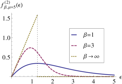
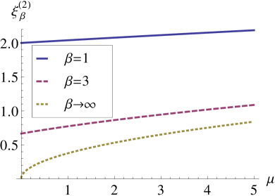
In Appendix A, we find $\mathbb{E}\log\Xi$ from which the following two quantities can be directly calculated. First, the expected number of edges in the grand canonical ensemble is

$$\mathbb{E}|E(G)|=\mathbb{E}[\mathbb{E}[|E(G)|\,|V_{nD}]]=\mathbb{E}\frac{\partial\log\Xi}{\partial\log\kappa} =\frac{\partial\mathbb{E}\log\Xi}{\partial\log\kappa}$$

$$=\frac{n}{2}\frac{S_{D-1}}{\beta^{D}}\,\Gamma(D)\,\left[-\mathrm{Li}_{D}(-\kappa)\right]\,,$$ (8)

where $S_{D-1}=D\pi^{\frac{D}{2}}/\Gamma(1+\frac{D}{2})$ is the area of the unit $(D-1)$-sphere, and $\mathrm{Li}_{s}(z)=\sum_{k=1}^{\infty}z^{k}/k^{s}$ is the Polylogarithm function. In order that the grand canonical ensemble description be equivalent to the ESNM, we need to set $\mathbb{E}|E(G)|$ equal to the number of edges $n\mu/2$ in the ESNM. This means

$$\mu=\frac{S_{D-1}}{\beta^{D}}\,\Gamma(D)\,\left[-\mathrm{Li}_{D}(-\kappa)\right]\,.$$ (9)

In the rest of the section we will treat $\kappa=\kappa_{\beta\mu}^{(D)}$ to be implicitly defined through (9), and $g(\cdot)=g_{\beta\mu}^{(D)}(\cdot)$.

Second, the expected value of the network Hamiltonian, i.e., the expected total length of the network is

$$\mathbb{E}H(G)=-\frac{\partial\mathbb{E}\log\Xi}{\partial\beta}=\frac{n}{2}\frac{S_{D-1}\Gamma(D+1)}{\beta^{D+1}}\left[-\mathrm{Li}_{D+1}\left(-\kappa_{\beta\mu}^{(D)}\right)\right]\,.$$ (10)

The mean edge length $\xi=\mathbb{E}[H(G)/|E(G)|]$. When $n\to\infty$, both $H(G)/n$ and $|E(G)|/n$ will converge to their respective limits, so that

$$\xi=\xi_{\beta\mu}^{(D)}\to\frac{\mathbb{E}H(G)}{\mathbb{E}|E(G)|}=\frac{S_{D-1}\Gamma(D+1)}{\mu\beta^{D+1}}\left[-\mathrm{Li}_{D+1}\left(-\kappa_{\beta\mu}^{(D)}\right)\right]\,.$$ (11)

To find the distribution of vertex degrees and edge lengths it is more convenient to use the percolation picture. Since the neighbors of a vertex are assigned independently of each other with a probability that depends on distance, the degree distribution is Poisson (for a proof see Appendix B). Next we consider the distribution of the lengths of the edges in the network. We want to find the probability

$$\mathbb{P}(|x-y|=\varepsilon|\{x,y\}\in E) =\frac{\mathbb{P}(\{x,y\}\in E||x-y|=\varepsilon)\mathbb{P}(|x-y|=\varepsilon)}{\mathbb{P}(\{x,y\}\in E)}$$

$$=\frac{g_{\beta\mu}^{(D)}(\varepsilon)\mathbb{P}(|x-y|=\varepsilon)}{\int g_{\beta\mu}^{(D)}(\varepsilon^{\prime})\mathbb{P}(|x-y|=\varepsilon^{\prime})}\,.$$ (12)

As $n\to\infty$, $\mathbb{P}(|x-y|=\varepsilon)\to S_{D-1}\varepsilon^{D-1}\mathrm{d}\varepsilon/n$. Substituting in (12), we get the probability density function of the distribution of edge lengths to be (see Fig. 1(a))

$$f_{\beta\mu}^{(D)}(\varepsilon)=S_{D-1}\frac{g_{\beta\mu}^{(D)}(\varepsilon)\varepsilon^{D-1}}{\mu}\,.$$ (13)

(a) $\beta=0$

(b) $\beta\to\infty$

Figure 2: Pictures of the (a) Erdős-Rényi graph, and (b) the random geometeric graph, on a square with $n=1000$ vertices.

The two extreme values of $\beta$ deserve special consideration. With $\beta=0$, the spatial location of the vertices have no effect on the evolution of the network and so the equilibrium network is the Erdős-Rényi graph (a random graph drawn uniformly from the set of networks with a given number of vertices and edges) of which the degree distribution, the formation of the giant component, clustering coefficient, etc. are well known newman10 . As $n\to\infty$, the mean edge length grows as the mean vertex pair distance which is $\mathcal{O}(n^{1/D})$. Note that this is consistent with the fact that $\lim_{\beta\to 0}\xi_{\beta\mu}^{(D)}=\infty$ for all $D$, $\mu>0$.

In the limit of large $\beta$, the rewiring algorithm becomes a greedy algorithm that always chooses the shorter edge. The equilibrium network will then be a random geometric graph (RGG) Dall2002 ; Penrose2003 where vertices are connected to all their spatial neighbors up to a distance $\varepsilon_{0}$, equal to the $|E|$-th smallest distance between vertices. Alternatively, $\varepsilon_{0}$ is the Fermi energy of the system. This means

$$\binom{n}{2}\mathbb{P}(|x-y|<\varepsilon_{0}) =|E|\,.$$ (14)

So as $n\to\infty$, we have

$$\binom{n}{2}\int_{0}^{\varepsilon_{0}}\frac{1}{n}S_{D-1}\varepsilon^{D-1}\mathrm{d}\varepsilon=n\frac{\mu}{2}\quad\hbox{which means}\quad\Omega_{D}\varepsilon_{0}^{D}=\mu\,,$$ (15)

where $\Omega_{D}=\pi^{\frac{D}{2}}/\Gamma(1+D/2)$ is the volume of a unit $D$- ball. The mean edge length is

$$\xi_{\beta\to\infty,\mu}^{(D)}=\int_{0}^{\varepsilon_{0}}\varepsilon\,\frac{S_{D-1}\varepsilon^{D-1}\mathrm{d}\varepsilon}{\Omega_{D}\varepsilon_{0}^{D}}=\frac{S_{D-1}}{(D+1)\Omega_{D}}\varepsilon_{0}=\frac{D}{(D+1)\Omega_{D}^{\frac{1}{D}}}\mu^{1/D}\,.$$ (16)

The clustering coefficient $C$ is defined as the probability that two vertices that are connected to a common third vertex are also connected to each other, i.e., for three randomly chosen vertices $x$, $y$ and $z$, $C=\mathbb{P}(\{x,z\}\in E|\{x,y\},\{y,z\}\in E)$. Spatial networks should be expected to have high clustering, since two spatial neighbors of a vertex are also spatial neighbors of each other. For the percolation network, the clustering coefficient is

$$C=\frac{\int\int g(|x|)\,g(|y|)\,g(|x-y|)\,\mathrm{d}x\,\mathrm{d}y}{\int\int g(|x|)\,g(|y|)\,\mathrm{d}x\,\mathrm{d}y}\,.$$ (17)

For general values of $\beta$, it is difficult to evaluate (17). However, in the $\beta\to\infty$ limit, $C$ can be calculated as given in Dall2002 and found to be (see Appendix C)

$$C_{\beta\to\infty,\mu}^{(D)} =\frac{2D^{2}}{\sqrt{\pi}}\frac{\Gamma(D/2)}{\Gamma((D+1)/2)}\int_{0}^{1}\int_{0}^{\arccos(t/2)}\sin^{D}\tau\,\mathrm{d}\tau\,t^{D-1}\,\mathrm{d}t\,.$$ (18)

Notice that $C_{\beta\to\infty,\mu}^{(D)}$ is independent of the mean degree $\mu$.

(a)

Figure 3: Fraction of vertices $\rho$ in the largest component (a) as a function of $\mu$ for various values of $\beta$ and (c) as a function of $\beta$ for various values of $\mu$. (b) shows the finite size scaling for $\beta=3$; notice that all the curves seem to cross at one point.

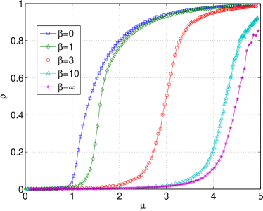
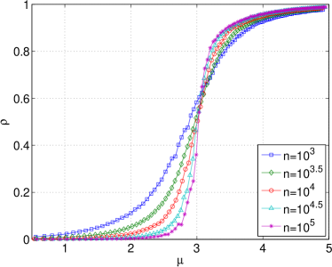
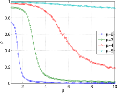
It does not seem possible to analytically compute the size of the giant component in the percolation network. Because of this, we simulate the percolation process. In all the results that follow, the dimension $D=2$, and, unless otherwise stated, the network size $n=10^{4}$.

For fixed $\beta$, when $\mu$ is varied, the equilibrium network undergoes a percolation transition (in the $n\to\infty$ limit), indicated by the fraction $\rho$ of vertices in the giant component. For $\beta=0$, we know that the critical mean degree $\mu_{{*}}^{(\beta=0)}=1$ for formation of the giant component (see Fig. 3). Increasing $\beta$ makes the formation of the largest component difficult, as long connections are not favored. However, there is an upper bound on $\mu_{{*}}$ achieved when $\beta\to\infty$ and the network is an RGG. Our simulation shows this bound to be $\mu_{{*}}^{(\beta\to\infty)}\approx 4.5$, in agreement with the simulation result reported in Dall2002 . For $\beta=3$, the critical mean degree for percolation appears to be $\mu_{{*}}^{(\beta=3)}\approx 3.1$ from the crossing point of the curves corresponding to different network sizes in Fig. 3. Fig. 3(a) shows the size of the largest component as function of $\beta$ for fixed values of $\mu$. Consistent with Fig. 3, we see that for $\mu<\mu_{{*}}^{(\beta\to\infty)}$ there is a maximum $\beta=\beta_{*}$ for the existence of a giant component, while for $\mu>\mu_{{*}}^{(\beta\to\infty)}$ there is a giant component for all values of $\beta$.

Figure 4: Clustering coefficient as a function of $\mu$ for various values $\beta$. (The non-uniform distribution of data points in $\mu$ correspond to uniform data points in $\kappa_{\beta\mu}^{(D)}$.)

For a given $\mu$, the clustering of vertices increases as $\beta$ increases, achieving the maximum value as $\beta\to\infty$ (see Fig. 4). Substituting $D=2$ in (18), we find that $C=1-3\sqrt{3}/4\pi\approx 0.59$.

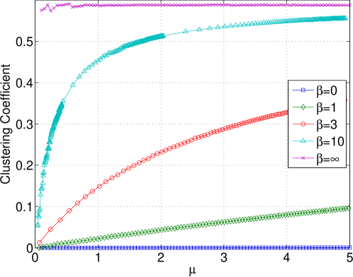
II.3 A model for a social network

The unconstrained model can be used as a model of a social network where the individuals have fixed opinions on $D$ number of issues. The parameter $\beta$ represents the tendency of individuals to befriend others of opinions similar to theirs, also known as homophily. The limitation in the number of active social contacts an average person can maintain is represented by the fixed value of the mean degree $\mu$. With the above interpretation of the parameters, the properties of the unconstrained ESNM are compatible with those of real social networks. First, clustering, which is a central feature of any social network is easily captured by the model (Fig. 4).

Second, the absence of a giant component would imply a fragmented social network (Fig. 3). So the critical mean degree $\mu_{*}^{(\beta)}$ is the minimum number of friends that individuals need to make, so that a positive fraction of the social network is connected. The stronger the preference of individuals to connect to similar individuals (i.e., large $\beta$), the larger the number of friends they need to make (large $\mu$) to prevent disintegration. However, even with a very high homophily, if the number of friends is at least $\mu_{{*}}^{(\beta\to\infty)}\approx 4.5$, the social network is guaranteed to be have a giant component.

The probability of an edge from a vertex to its spatial neighbor decreases with the distance. Since the density of vertices is constant for $D=1$, but increasing with distance for $D\geq 2$, the corresponding edge length distributions have a maxima at zero and at a positive value, respectively. For the social network, this implies that when there is only a single issue on which opinions matter, the individuals mostly connect to others with opinions very close to theirs. On the other hand, when individuals choose their friends based on their opinions on multiple issues, the highest concentration of friends is found at a positive opinion difference.

III The Connected ESNM

(a) $\mu=2$

(b) $\mu=4$

Figure 5: A realization of the almost optimized network ($\beta=10$)for two different values of the mean degree. The red circles and blue lines correspond to the vertices and edges respectively

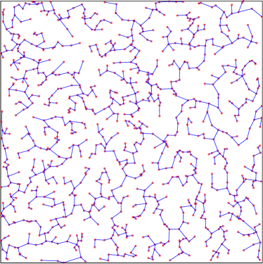
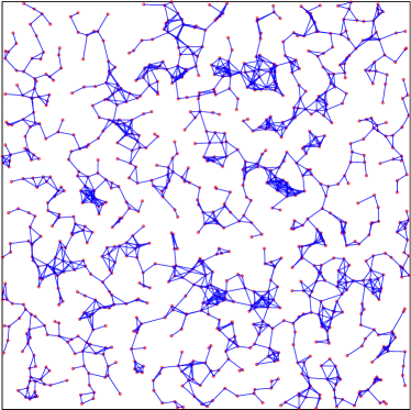
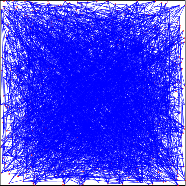
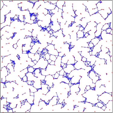
We now consider our model with the constraint $\mathcal{T}$ that the network be connected. Such a requirement is natural for many real world networks, for e.g., airline networks, road networks Barrat2005 . Although, we know the equilibrium distribution (4) of the network, it is difficult to proceed further analytically as we can no longer define an equivalent percolation version of the model as we did for the unconstrained model. The connectedness constraint makes the edges of the equilibrium network highly correlated. Therefore we study the connected ESNM purely by simulation. For simplicity, we will focus on two cases: when the parameter $\beta$ is zero and when it takes a large value 10. We will refer to the $\beta=0$ equilibrium network as the Random Connected Network or RCN($\mu$), and for reasons that will be elucidated in Section III.2, the $\beta=10$ network will be called the Almost Optimized Network or AON($\mu$).

For the simulation we choose the dimension $D=2$. Since it is computationally costly to verify that the network remains connected, we will reduce our simulation size for the connected network to $n=10^{3}$ The initial network is formed by randomly ordering the vertices and adding $n-1$ edges to form a chain. The remaining $n\mu/2-(n-1)$ edges are randomly chosen from the remaining vertex pairs. We say that equilibrium has been reached when the mean edge length changes by less that 0.5% across time points separated by a large number (1000 times the number of edges) of network update attempts. Fig. 5 shows the network for two values of the mean degree.

III.1 Mean edge length, degree distribution, and clustering

Figure 6: Mean edge length $\xi$ of the AON.

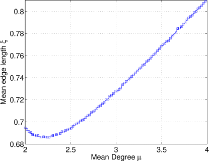
As in the unconstrained case, the mean edge length blows up in the RCN for $n\to\infty$. The mean edge length as a function of $\mu$ for the AON is shown in Fig. 6. It is interesting to note that that $\xi(\mu)$ is not monotone, but achieves a minima around $\mu=2.2$. As $\mu$ increases from 2 until about 2.5, the increase in the total length of the network seems to be overcompensated by the increased flexibility in keeping the network connected, resulting in short edge lengths.

(a) RCN

(b) AON

Figure 7: Degree distribution of the random connected and optimized networks.

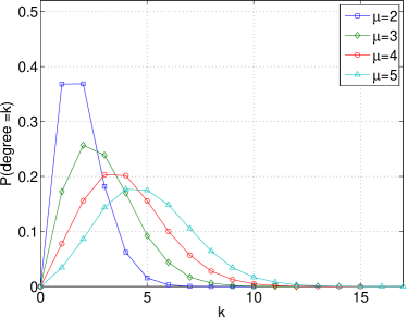
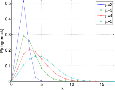
In contrast to the unconstrained network, the degree distribution of the connected network does not appear to be Poisson for any value of $\beta$, as seen in Fig. 7. The distribution however is still peaked around the mean with a thin tail. For $\mu=2$, the AON has a markedly higher peak at $2$ than the RCN.

Figure 8: Clustering coefficient as a function of the mean degree $\mu$.

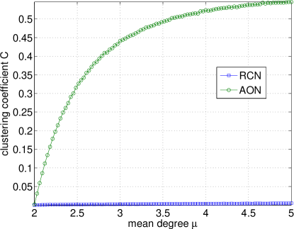
For the RCN, since the spatial locations are unimportant, it is natural that the clustering coefficient vanishes (as $n\to\infty$). The AON, on the contrary, has high clustering as shown in Fig. 8.

III.2 The $\beta\to\infty$ model as an optimization process

In the $\beta\to\infty$ limit, the connected ESNM may be viewed as a stochastic algorithm (although not a very efficient one) to solve the following optimization problem: Given a collection of $n$ points uniformly distributed in $\mathcal{V}_{nD}$ and $\mu\geq 2-2/n$ (i.e., the number of edges is at least the minimum $n-1$ needed to connect $n$ vertices), find the connected spatial network $G_{*}$ with mean degree $\mu$ that has the lowest total length, i.e., find

$$G_{*}(\mu)=\underset{G\in\mathcal{G}_{c}(V_{nD},\mu)}{\arg\max}H(G)\,,$$ (19)

where $\mathcal{G}_{c}(V_{nD},\mu)$ is the set of connected networks with vertex set $V_{nD}$ and $n\mu/2$ edges

Now, consider the general problem of finding an “efficient” network over a given collection of points. Obviously, the application one is interested in determines the optimization metric Thai2012 . A simple and very popular optimal network is the minimum spanning tree abbreviated as MST (see Graham1985 for a history and Prim1957 for a classic algorithm). Here the quantity that is minimized is the total length, or equivalently, the “wiring cost” of the network. $G_{*}(\mu)$ is very similar to the MST with the notable exception that it is not a tree for $\mu\geq 2$. Indeed, $G_{*}(\mu=2-2/n)$ is the MST.

However, one could potentially be concerned about other aspects of the network in addition to its wiring cost, and a tree may no longer be a good option. For example, Aldous Aldous2008b ; Aldous2010 sought networks which in addition to minimizing the wiring cost also has short routes, i.e., the route distance between any pair of vertices is close to their spatial distance. He quantified this property by defining the route factor $R(x,y)$ between two vertices $x$ and $y$ as

$$R(x,y)=\frac{r(x,y)}{|x-y|}-1\,,$$ (20)

where $r(x,y)$ is the route distance or the length of the shortest route between $x$ and $y$. The route factor defined for a single vertex pair can then be averaged over all vertex pairs to arrive at a useful statistic for the network – the mean route factor $R$. Gastner and Newman Gastner2006 studied a growth model for spatial networks, where given a $V_{n2}$ (i.e., vertices distributed uniformly in a square) with a designated “root” vertex, a connected cluster is grown by sequentially adding edges to vertices outside the cluster; the edges are chosen according to a greedy optimization criterion that minimizes a linear combination of the new edge length, and the route factor between the new and the root vertices.

One may also want the network to be robust to random failures of its edges. One way to test this kind of robustness of a connected network is by randomly removing edges He2009 and noting the size of the largest component of the resulting network. Specifically, for a connected network of mean degree $\mu$ we look at the fraction $\rho_{\mu}(\mu^{\prime})$ of vertices in the largest component when the edge removal leads to a network of mean degree $\mu^{\prime}$. A robust network should retain a large fraction of its vertices in its largest component when $\mu^{\prime}$ decreases from $\mu$; in other words the function $\rho_{\mu}(\mu^{\prime})$ should be concave downwards for a sizeable region near $\mu^{\prime}=\mu$. We thus quantify the robustness of the network by the inflection point $\tilde{\mu}(\mu)$ of the $\rho_{\mu}(\cdot)$ curve. Note that lower $\tilde{\mu}(\mu)$ means more robust. The $\rho_{\mu}(\cdot)$ curve may always be convex indicating the lack of robustness of the network; therefore, for a collection of networks parametrized by their mean degrees $\mu$, we define the critical mean degree $\mu_{*}$ for robustness as the smallest $\mu$ for which there exists an inflection point.

Thus, similar to Tero2010 , we characterize the efficiency of a given network of mean degree $\mu$, by three statistics: the scaled total edge length $\chi=H(G)/n^{1+1/D}$, the route factor $R$, and $\tilde{\mu}$. The smallness of all these network statistics is desirable for an efficient network. How does $G_{*}(\mu)$ fare in these measures of efficiency? In order to get an approximation to $G_{*}(\mu)$, we perform simulations using $\beta=10$ and term the equilibrium network as the almost optimized network or AON($\mu$). Since the equilibrium of the $\beta=0$ connected model is uniformly drawn from the set $\mathcal{G}_{c}(V_{nD},\mu)$ without regard for the edge length, it can be viewed as a null model for comparison with the AON, and we will refer to it as the Random Connected Network or RCN($\mu$).

(a) RCN

(b) AON

Figure 9: The route factor $R$ versus the scaled total length $\chi$ for the RCN and the AON.

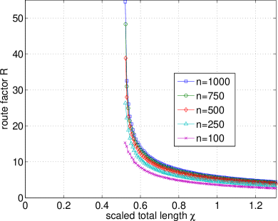
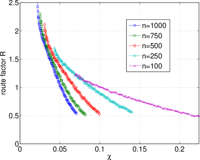
The two opposing statistics – route factor and scaled total length, are plotted against each other in Fig. 9(a) and 9(b) to get convex “efficiency curves”, which show that the AON is significantly more efficient than the RCN if we only take $\chi$ and $R$ into account. The finite size scaling shows that the route factor diverges at $\chi\approx 0.52$ for the RCN corresponding to the random connected tree, and at $\chi\approx 0.02$ for the AON corresponding to the MST.

Figure 10: Robustness of the (a) RCN and (b) AON.

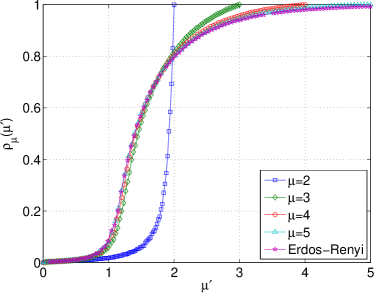
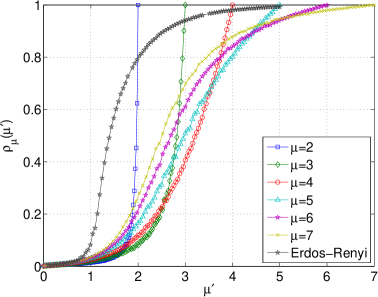
However, in terms of robustness to random edge failures, the RCN with its abundance of long range connections performs better as shown in Fig. 10. For comparison, we also include the fraction of vertices in the largest component of an Erdős-Rényi random graph (note than an ER graph with edges removed at random is just another ER graph with a lower mean degree). While it is difficult to precisely locate the inflection point $\tilde{\mu}(\mu)$ in these curves, it is easy to see that it decreases with increase in the mean degree $\mu$, i.e., as one would expect, more edges make the network more robust. In Fig. 10, the $\mu=3,4,5$ curves are almost indistinguishable from the ER curve and show the percolation transition close to $\mu^{\prime}=1$, indicating that they are very similar to Erdős-Rényi networks. However, the behavior of the Almost Optimized Networks as seen in Fig. 10 is quite different. It can be inferred from Fig. 10 that the critical mean density $\mu_{*}=2$ for the RCN, and $4<\mu_{*}<5$ for the AON.

Figure 11: Mean route distance $r$ versus mean hop distance $h$ for the RCN and AON.

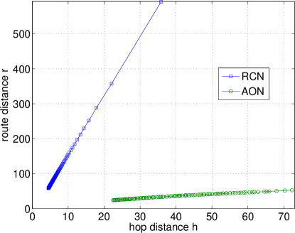
The mean route distance $r$ is lower for the AON than for the RCN; however, in achieving a lower $r$, the AON gets a higher mean hop distance $h$ (Fig. 11).

III.3 Testing the model on real data

In this section, we apply the connected ESN model on two sets of data, to gain some insight into the applicability of the model.

Figure 12: Pictures generated using the Minnesota road network data – (a) the actual network, and (b) the simulated network with $\beta=50$.

	Data	Simulation
mean edge length $\xi$	0.0683	0.0517
clustering $C$	0.0280	0.114
hop distance $h$	80.0	76.8
route distance $r$	6.10	5.76
route factor $R$	1.79	1.64

Table 1: Comparison of various statistics of the actual and simulated networks.

Figure 13: Comparison of (a) robustness and (b) degree distribution, of the actual, simulated, and Erdős-Rényi networks.

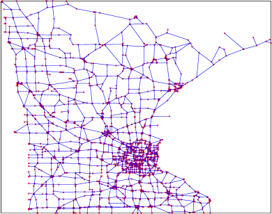
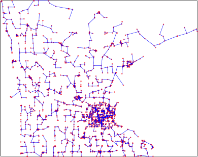
Our first data set is about the network of roads in the US state of Minnesota, obtained from minnesota . There are $n=2635$ vertices in this network which correspond to the intersections of the roads. The mean degree is $\mu\approx 2.5$. To obtain the simulated network, we run the connected ESNM on the vertex set of the actual network, with the same mean degree and a large $\beta=50$.

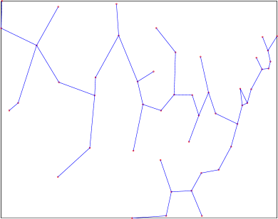
In Fig. 12 we see that the actual and simulated networks look very different. While the actual network has a grid like structure almost throughout, the simulated network is tree like for the most part, expect for the small region (which corresponds to the capital city of Minneapolis) with a very high density of vertices. Table 1 compares the two network using the statistics we used earlier, and we find that the simulated network performs better than the actual network on all of them. Specifically, the hop and route distances, and the route factor, which are all measures of the ease of traversing the network, are marginally lower. Also for the simulated network, the construction cost of the roads measured by the mean edge length is slightly lower, while the clustering coefficient is significantly higher.

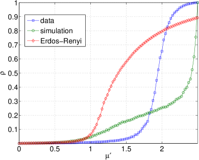
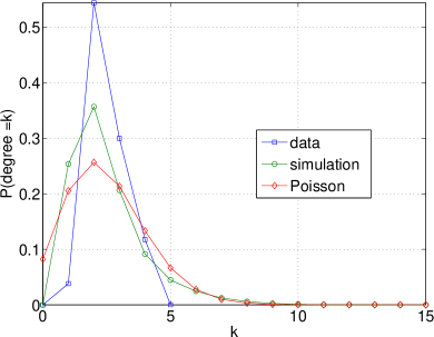
So does this mean that the simulated network is the more “efficient” and “better” network? It does not seem likely that people living along the border with Canada would agree. In the “optimized” network they often have to go large distances to get to a nearby town, and even if they are driving to Minneapolis, they have a much longer route. Second, how robust are the two networks to edge failures? Fig. 13 shows that the simulated network is extremely fragile compared to the actual network; a loss of less than 8% of the edges is enough to bring the size of the largest component down to a third of the network size. The actual network, on the contrary, is robust (by our earlier definition) with a $\tilde{\mu}\approx 1.9$. Fig. 13 shows that in the actual network, a large fraction of the intersections are created by two roads, and no intersection is made of more than four roads – both of which are unsurprising. The simulated graph, while having a peak at 2, has unrealistic 9-road intersections in the capital region.

The undesirable topology of the simulated network can be attributed mainly to the highly non-uniform distribution of vertices in the graph (recall that our model assumes a uniform distribution of the vertices). Our connected ESNM allocates a disproportionate amount of edges to regions of high vertex density. One may also argue about the quality of the statistics we used; specifically, in practical applications, extreme values of the hop and route distances and route factor are perhaps more relevant than their averages. Nevertheless, our robustness measure seems to be a reliable statistic for most cases.

(a) $\mu=2$

(b) $\mu=3$

Figure 14: Pictures of connected ESNM on US the state capitals” locations for two values of the mean degree.

	$\mu=2$	$\mu=2.2$	$\mu=3$	$\mu=4$
mean edge length $\xi$	2.70	2.66	2.75	2.932
clustering $C$	0.045	0.178	0.425	0.539
hop distance $h$	9.20	8.90	6.94	5.54
route distance $r$	24.1	23.8	21.2	19.1
Route factor $R$	0.633	0.606	0.382	0.234

Table 2: Statistics obtained for the ESNM on US state capitals’ locations with three values of the mean degree and $\beta=50$.

Figure 15: Comparison of (a) robustness and (b) degree distribution, of simulation results for US state capitals’ locations data for four values of $\mu$.

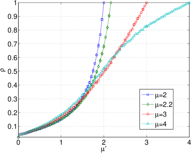
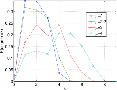
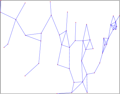
Our next test bed for the connected ESNM is the locations of the lower 48 US state capitals. Here, the vertices are more uniformly distributed than in the the road network we considered earlier. Nonetheless, Fig. 14(b) shows the accumulation of edges when $\mu=3$, in the north east region where there are many states. In Table 2 shows that, as is to be expected, the clustering coefficient and all the distance measures decrease when $\mu$ increases. The mean edge length, however, is non-monotone, consistent with our earlier findings shown in Fig. 6. The robustness profile in Fig. 15 shows that the $\mu=4$ network is robust by our criterion, while $\mu=2$ and 3 are not, i.e., $3<\mu_{*}<4$. Fig. 15 shows the degree distribution; the bimodality of the curve for $\mu=3$ and 4 is peculiar and is perhaps due to the inhomogeneous distribution of points.

IV Summary and Outlook

In this paper we have introduced an abstract model for the evolution of spatial networks whose equilibrium distribution is given by an explicit formula containing their spatial dimension, their mean degree, the topological constraint and the inverse temperature $\beta$. We examined two cases – one where the topological constraint is absent, and the other where the network is required to be connected.

The unconstrained network is closely related to a percolation problem. This enabled us to analytically compute the distribution of the degrees and edge lengths, and the clustering coefficient of the network. Other quantities such as the critical mean degree $\mu_{*}^{(\beta\to\infty)}$ for percolation were estimated by simulation. One interesting aspect of this model is that that it interpolates between the Erdős-Rényi random graph ($\beta=0$) and the random geometric graph ($\beta=\infty$). Furthermore, the unconstrained ESNM can be a model for a social network where stubborn individuals with fixed opinions a number of issues, have a tendency to rewire their ties to those with similar opinions. Even when this tendency was high, the fact that the number of edges is fixed, ensured that a small mean degree was enough to have a giant component.

An analytical framework for computing quantities associated with the connected network model is lacking, so we studied that model purely by simulation concentrating on the random connected network ($\beta=0$) and the almost optimized network ($\beta=10$). Our analysis focused on the total length (‘wiring cost’) of the network, how routes between vertices compare with their spatial separation, and the robustness of the network to random removal of edges. In the former two aspects, we found that the almost optimized network is notably more efficient than the random connected network. However, in terms of the metric that we proposed, the RCN was found to be more robust. A peculiar feature we noted of the AON($\mu$) is that the mean edge length is the lowest when $\mu\approx 2.2$, and not at 2 as one would expect.

To test the success of our second model for network design we considered two examples: the Minnesota road network and the 48 state capitals of the continental US. While the rewiring produced networks with good values of some important statistics, additional criteria (e.g., reweighted edges based on population density to compensate for uneven vertex distributions) will need to be introduced to produce good solutions.

Appendix A The grand partition function

It is well known (see for e.g. Pathria2007 ) that the grand partition function of non-interacting particles can be written as a product over single particle states. So, in our case, we have

$$\Xi(\beta,\kappa)=\prod_{\{x,y\}\in\binom{V}{2}}\left(1+\kappa e^{-\beta|x-y|}\right)\,.$$ (21)

Since the partition functions above are conditional on the location of the vertices, we calculate the expected value

$$\mathbb{E}\log\Xi =\left[\prod_{x\in V}\int_{\mathcal{V}_{nD}}\frac{\mathrm{d}x}{n}\right]\sum_{\{x,y\}\in\binom{V}{2}}\log\left(1+\kappa e^{-\beta|x-y|}\right)$$

$$=\binom{n}{2}\int_{\mathcal{V}_{nD}}\int_{\mathcal{V}_{nD}}\frac{\mathrm{d}x}{n}\frac{\mathrm{d}y}{n}\log\left(1+\kappa e^{-\beta|x-y|}\right)\,.$$ (22)

In the limit of large $n$, the double integration in (22) is to be performed over $\mathbb{R}^{2D}$ and all points are identical. We can choose a point at $x$. Then calculate $\int g(|x-y|)\mathrm{d}y$, by constructing shells centered at $x$ at all radii $\varepsilon$. This quantity will be independent of $x$. The remaining integral $\int\mathrm{d}x/n$ is just equal to 1, giving

$$\mathbb{E}\log\Xi =\frac{n}{2}S_{D-1}\int_{0}^{\infty}\varepsilon^{D-1}\log\left(1+\kappa e^{-\beta\varepsilon}\right)\mathrm{d}\varepsilon=\frac{n}{2}\frac{S_{D-1}\Gamma(D)}{\beta^{D}}[-\mathrm{Li}_{D+1}(-\kappa)]\,.$$ (23)

Appendix B Degree distribution in the percolation network

We can calculate the degree distribution of the percolation network as follows. Let $X$ be a randomly chosen vertex and let $Y$ be one of the other vertices. The probability that $X$ is connected to $Y$ is

$$\mathbb{P}(\{X,Y\}\in E)=\int\mathbb{P}(\{X,Y\}\in E|Y=y)\mathbb{P}(Y=y)=\frac{1}{n}\int g(|X-y|)\mathrm{d}y\,.$$

The probability that $X$ is connected to exactly $k$ of the other $n-1$ vertices is

$$\mathbb{P}(d(X)=k) =\mathrm{Binomial}\left(n-1,\mathbb{P}(\{X,Y\}\in E);k\right)$$

$$=\mathrm{Binomial}\left(n-1,\frac{1}{n}\int g(|X-y|)\mathrm{d}y;k\right)$$

$$\to\mathrm{Poisson}\left(\int g(|X-y|)\mathrm{d}y;k\right)\quad\textrm{as}\quad n\to\infty\,.$$ (24)

So a vertex at $x$ has a degree distribution $\mathrm{Poisson}[\mu(x)]$ where $\mu(x)=\int g(|x-y|)\mathrm{d}y$.

Appendix C Clustering Coefficient for $\beta\to\infty$

Consider a vertex $z$ that is connected to vertices $x$ and $y$. This means that $x$ and $y$ lie within a $D-$ball of radius $\varepsilon_{0}$ centered at $z$. Now, $x$ and $y$ will be connected to each other only if $y$ lies in the intersection of the $D-$balls of radii $\varepsilon_{0}$ centered at $x$ and $z$ respectively. In other words, the probability that $y$ is connected to $x$ is the ratio of the intersection volume of the $D-$balls to the volume of a $D-$ball. The volume of the cap that subtends a half angle $\theta$ of a unit $D$-ball is given by

$$\Omega_{D}^{\textrm{cap}}(\theta)=\frac{\pi^{\frac{D-1}{2}}}{\Gamma\left(\frac{D+1}{2}\right)}\int_{0}^{\theta}\sin^{D}t\,\,\mathrm{d}t\,.$$ (25)

If $|x-z|=\varepsilon<\varepsilon_{0}$, to find the intersection volume, we need to add the volumes of two such caps with $\theta=\arccos(\varepsilon/2\varepsilon_{0})$. The probability that $|x-z|=\varepsilon$ is $S_{D-1}\varepsilon^{D-1}\mathrm{d}\varepsilon/\Omega_{D}\varepsilon_{0}^{D}$. So averaging the intersection volume over all $\varepsilon$, we have,

$$C =\frac{1}{\Omega_{D}\varepsilon_{0}^{D}}\int_{0}^{\varepsilon_{0}}2\Omega_{D}^{\textrm{cap}}\left(\arccos\left(\frac{\varepsilon}{2\varepsilon_{0}}\right)\right)\varepsilon_{0}^{D}\frac{S_{D-1}\varepsilon^{D-1}\mathrm{d}\varepsilon}{\Omega_{D}\varepsilon_{0}^{D}}$$

$$=\frac{2D^{2}}{\sqrt{\pi}}\frac{\Gamma(D/2)}{\Gamma((D+1)/2)}\int_{0}^{1}\int_{0}^{\arccos(t/2)}\sin^{D}\tau\,\mathrm{d}\tau\,t^{D-1}\,\mathrm{d}t\,.$$ (26)

References

- [1] Mark E. J. Newman. The Structure and Function of Complex Networks. SIAM Review, 45:167–256, January 2003.
- [2] Feng Xie and David Levinson. Modeling the Growth of Transportation Networks: A Comprehensive Review. Networks and Spatial Economics, 9(3):291–307, October 2007.
- [3] David J. Aldous. Optimal spatial transportation networks where link costs are sublinear in link capacity. Journal of Statistical Mechanics: Theory and Experiment, 2008(03):P03006, March 2008.
- [4] David J. Aldous. Spatial transportation networks with transfer costs: asymptotic optimality of hub-and-spoke models. Mathematical Proceedings of the Cambridge Philosophical Society, 145(02):471–487, April 2008.
- [5] Atsushi Tero, Seiji Takagi, Tetsu Saigusa, Kentaro Ito, Dan P Bebber, Mark D Fricker, Kenji Yumiki, Ryo Kobayashi, and Toshiyuki Nakagaki. Rules for biologically inspired adaptive network design. Science, 327(5964):439–42, January 2010.
- [6] Rémi Louf, Pablo Jensen, and Marc Barthelemy. Emergence of hierarchy in cost-driven growth of spatial networks. Proceedings of the National Academy of Sciences of the United States of America, 110(22):8824–9, May 2013.
- [7] Michael T. Gastner and Mark E. J. Newman. Shape and efficiency in spatial distribution networks. Journal of Statistical Mechanics: Theory and Experiment, 2006(01):P01015–P01015, January 2006.
- [8] Gerald F. Frasco, Jie Sun, Hernán D. Rozenfeld, and Daniel Ben-Avraham. Spatially Distributed Social Complex Networks. Physical Review X, 4(1):011008, January 2014.
- [9] Ed Bullmore and Olaf Sporns. Complex brain networks: graph theoretical analysis of structural and functional systems. Nature reviews. Neuroscience, 10(3):186–98, March 2009.
- [10] Ed Bullmore and Olaf Sporns. The economy of brain network organization. Nature reviews. Neuroscience, 13(5):336–49, May 2012.
- [11] Danielle S. Bassett, Nicholas F. Wymbs, Mason A. Porter, Peter J. Mucha, Jean M. Carlson, and Scott T. Grafton. Dynamic reconfiguration of human brain networks during learning. Proceedings of the National Academy of Sciences of the United States of America, 108(18):7641–6, May 2011.
- [12] Marc Barthélemy. Spatial networks. Physics Reports, 499(1-3):1–101, February 2011.
- [13] B.M. Waxman. Routing of multipoint connections. IEEE Journal on Selected Areas in Communications, 6(9):1617–1622, 1988.
- [14] Duncan J. Watts and Steven H. Strogatz. Collective dynamics of ‘small-world’networks. Nature, 393(6684):440–442, 1998.
- [15] L. Barnett, E. Di Paolo, and S. Bullock. Spatially embedded random networks. Physical Review E, 76(5):056115, November 2007.
- [16] Olaf Sporns. Networks of the Brain. MIT Press, 2010.
- [17] S. Boccaletti, V. Latora, Y. Moreno, M. Chavez, and D.-U. Hwang. Complex networks: Structure and dynamics. Physics Reports, 424(4–5):175 – 308, 2006.
- [18] Nicholas Metropolis, Arianna W. Rosenbluth, Marshall N. Rosenbluth, Augusta H. Teller, and Edward Teller. Equation of State Calculations by Fast Computing Machines. The Journal of Chemical Physics, 21(6):1087, December 1953.
- [19] Adam Douglas Henry, Paweł Prałat, and Cun-Quan Zhang. Emergence of segregation in evolving social networks. Proceedings of the National Academy of Sciences, 108(21):8605–8610, 2011.
- [20] Sam R. Magura, Vitchyr He Pong, David Sivakoff, and Rick Durrett. Two evolving social network models. http://www.math.duke.edu/~rtd/NCSSM/evonets.html, 2013.
- [21] Mark E. J. Newman. Networks : An Introduction. Oxford University Press, Oxford New York, 2010.
- [22] Jesper Dall and Michael Christensen. Random geometric graphs. Physical Review E, 66(1):016121, July 2002.
- [23] Mathew Penrose. Random Geometric Graphs (Oxford Studies in Probability). Oxford University Press, USA, 2003.
- [24] Recall that the Fermi energy of a Fermionic system is the highest occupied single particle energy level at zero temperature.
- [25] Alain Barrat, Marc Barthélemy, and Alessandro Vespignani. The effects of spatial constraints on the evolution of weighted complex networks. Journal of Statistical Mechanics: Theory and Experiment, 2005(05):P05003, May 2005.
- [26] My T. Thai and Panos Pardalos. Handbook of Optimization in Complex Networks, volume 57 of Springer Optimization and Its Applications. Springer US, Boston, MA, 2012.
- [27] R.L. Graham and Pavol Hell. On the History of the Minimum Spanning Tree Problem. IEEE Annals of the History of Computing, 7(1):43–57, 1985.
- [28] R. C. Prim. Shortest Connection Networks And Some Generalizations. Bell System Technical Journal, 36(6):1389–1401, November 1957.
- [29] David J. Aldous and Wilfrid S. Kendall. Short-length routes in low-cost networks via Poisson line patterns. Advances in Applied Probability, 40(1):1–21, March 2008.
- [30] David J. Aldous and Julian Shun. Connected Spatial Networks over Random Points and a Route-Length Statistic. Statistical Science, 25(3):275–288, August 2010.
- [31] Shan He, Sheng Li, and Hongru Ma. Effect of edge removal on topological and functional robustness of complex networks. Physica A: Statistical Mechanics and its Applications, 388(11):2243–2253, June 2009.
- [32] http://www.cise.ufl.edu/research/sparse/matrices/Gleich/minnesota.html. Accessed on 04/25/2014.
- [33] Raj Kumar Pathria and Paul D. Beale. Statistical Mechanics, Third Edition. Academic Press, 2007.