Bayesian evidence of non-standard inflation:
Isocurvature perturbations and running spectral index

Abstract

Bayesian model comparison penalizes models with more free parameters that are allowed to vary over a wide range, and thus offers the most robust method to decide whether some given data require new parameters. In this paper, we ask a simple question: do current cosmological data require extensions of the simplest single-field inflation models? Specifically, we calculate the Bayesian evidence of a totally anti-correlated isocurvature perturbation and a running spectral index of the scalar curvature perturbation. These parameters are motivated by recent claims that the observed temperature anisotropy of the cosmic microwave background on large angular scales is too low to be compatible with the simplest inflation models. Both a subdominant, anti-correlated cold dark matter isocurvature component and a negative running index succeed in lowering the large-scale temperature power spectrum. We show that the introduction of isocurvature perturbations is disfavored, whereas that of the running spectral index is only moderately favored, even when the BICEP2 data are included in the analysis without any foreground subtraction.

I Introduction

Suppose that we wish to decide whether some data require the addition of a new parameter to a model. We may compare the logarithms of the likelihood values evaluated at the best-fit parameters. For example, the conventional $\chi^{2}$ method uses $\Delta\chi^{2}\equiv-2\ln({\cal L}_{1}/{\cal L}_{2})$. The obvious problem of this approach is that the addition of a new parameter is guaranteed to improve the fit, yielding a smaller $\chi^{2}$ value. But then, what does $\Delta\chi^{2}$ mean when we find, say, $\Delta\chi^{2}=-7$ by adding one more parameter? Do the data require such a parameter?

To address this issue, some criteria for comparing models have been discussed in the literature. The Akaike information criterion (AIC; Akaike (1974)) and the Bayesian information criterion (BIC; Schwarz (1978)) penalize models with more parameters by adding to $\chi^{2}$ a term proportional to the number of parameters. These criteria penalize all parameters equally regardless of predictability. For example, consider two parameters, one being allowed to vary from $-1$ to 1, and the other from 0 to $10^{10}$. While AIC and BIC penalize both parameters equally, a more sensible criterion should penalize the latter more strongly.

In this paper, we shall apply Bayesian model comparison Jeffreys (1961) to test whether extensions of the simplest inflation models are required by the current cosmological data. The Bayesian model comparison penalizes models with more free parameters that are allowed to vary over a wide range. Specifically, we compute the Bayesian evidence, ${\cal Z}$, defined by

$${\cal Z}\equiv\int d^{N}\theta~{}{\cal L}({\rm data}|{\bm{\theta}})P({\bm{\theta}}),$$ (1)

where ${\cal L}({\rm data}|{\bm{\theta}})$ is the likelihood of the data given the model parameters ${\bm{\theta}}$, and $P({\bm{\theta}})$ is the prior probability. We then compare two models by computing the logarithm of the ratio of their evidences, $\ln B\equiv\ln({\cal Z}_{1}/{\cal Z}_{2})$. Since the prior probability is normalized as $\int d^{N}\theta~{}P({\bm{\theta}})=1$, $P({\bm{\theta}})$ at a given set of $\bm{\theta}$ becomes small when a model contains more parameters varying over a wide range. This gives that model a small ${\cal Z}$, hence penalizing it more strongly. The factor $\ln B$ can be interpreted as the mathematical odds between the models given the data, which can also be expressed heuristically using the so-called “Jeffrey’s scale”, according to which the evidence for (or against) a model is said to be weak, moderate, and strong if $\ln B>1$, $2.5$, and $5$, respectively Trotta (2008). We shall adopt Jeffrey’s scale throughout this paper.

Why consider extensions of the simplest inflation models? Here, the “simplest inflation models” refer to inflation models driven by a single scalar field with a simple potential yielding approximately a power-law power spectrum of the scalar curvature perturbation.

A detection of isocurvature modes of any form would rule out all single-field inflation models. Moreover, a detection of a cold dark matter (CDM) isocurvature mode would shed light on the nature of CDM, e.g., axions Kolb and Turner (1990).

Given that the measured deviation of the scalar curvature power spectrum from scale invariance is $1-n_{s}\simeq 0.04$ Hinshaw et al. (2013a); Planck Collaboration (2014a), the running spectral index, $\rho_{s}\equiv dn_{s}/d\ln k$, is typically of order $(1-n_{s})^{2}={\cal O}(10^{-3})$; however, larger values are possible if the third derivative of the potential of a scalar field driving inflation is large Lyth and Riotto (1999). Thus, a large running index of order $10^{-2}$ necessarily requires a new energy scale in the potential (either in the kinetic term of the field Chung et al. (2003) or in the initial vacuum state Ashoorioon et al. (2014)), making the models more complicated.

A motivation to consider these extensions of the simplest single-field inflation models comes from the observational data of the cosmic microwave background (CMB). The Planck collaboration claims that the CMB temperature power spectrum data that they obtain at low multipoles are too low to be compatible with the best-fit power-law ($\rho_{s}=0$) adiabatic curvature perturbation spectrum Planck Collaboration (2014a). Both a negative running index and a nearly scale-invariant CDM isocurvature component that is anti-correlated with the curvature perturbation can lower the low-multipole power, reducing this apparent “tension” in the Planck temperature data Planck Collaboration (2014b).

This tension is exacerbated Smith et al. (2014), if a significant fraction of the B-mode polarization detected at degree angular scales by the BICEP2 collaboration BICEP2 Collaboration (2014) originates from the primordial, nearly scale-invariant gravitational waves generated during inflation, as such gravitational waves add extra power to the temperature power spectrum at low multipoles Starobinsky (1985). Then, do the Planck and BICEP2 data require either a negative running index or an anti-correlated CDM isocurvature perturbation? This is the question that we shall address in this paper using Bayesian model comparison.

Ref. Abazajian et al. (2014) computed the Bayesian evidence of a running index, showing that evidence for running is insignificant. Our results differ from theirs because of the choice of the data set and the prior probability on the amplitude of gravitational waves.

Refs. Hazra et al. (2014a, b, c); Meerburg (2014) computed $\Delta\chi^{2}$ for inflation models which produce modifications of the primordial power spectrum at small wavenumbers, but did not perform a Bayesian model comparison. Ref. Kawasaki et al. (2014) computed $\Delta\chi^{2}$ for isocurvature perturbations, but did not perform a Bayesian model comparison. Thus, they were unable to conclude whether the data require such extensions of the simple inflation models.

The structure of this paper is as follows: We describe the models in Section II, and present the data sets we use and the analysis method in Section III. We describe our results in Section IV, and conclude in Section V.

II Models

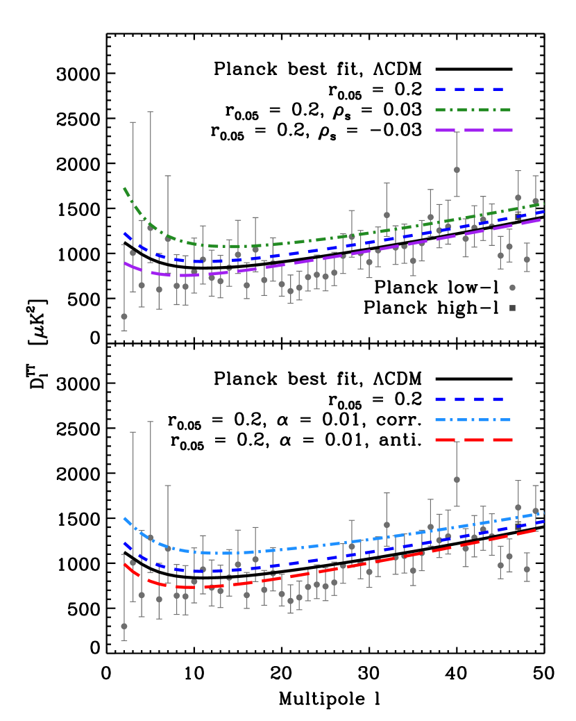
Figure 1: Comparison of the $\Lambda$CDM and extended models. In both panels, the solid lines show the scalar CMB power spectrum of the six-parameter $\Lambda$CDM model, while the short-dashed lines show the sum of the solid lines and the tensor power spectrum with a tensor-to-scalar ratio of $r_{0.05}=0.2$. The symbols with error bars show the Planck measurements Planck Collaboration (2014c). (Top panel:) The long-dashed and dot-dashed lines show the sum of the tensor power spectrum and the scalar power spectrum with negative and positive running indices, respectively, with $|\rho_{s}|=0.03$. (Bottom panel:) The long-dashed and dot-dashed lines show the sum of the short-dashed line and totally anti-correlated and correlated CDM isocurvature components, respectively, with an isocurvature-to-curvature ratio of $\alpha=0.01$.

II.1 Model I: Running scalar spectral index

We write the scalar curvature power spectrum as

$$\mathcal{P}_{\cal R}(k)=A_{s}\,\bar{k}^{n_{s}-1+\frac{1}{2}\rho_{s}\ln\bar{k}}\,,$$ (2)

where $n_{s}$ and $\rho_{s}$ are the scalar spectral index and its running, respectively, and $\bar{k}\equiv k/(0.05~{}{\rm Mpc}^{-1})$ is the normalized wavenumber. The tensor power spectrum is

$$\mathcal{P}_{h}(k)=r_{0.05}\,A_{s}\bar{k}^{-r_{0.05}/8}\,,$$ (3)

where $r_{0.05}$ is the tensor-to-scalar ratio defined at $k=0.05~{}{\rm Mpc}^{-1}$.

In the top panel of Fig. 1 we compare the temperature power spectrum data, $D_{l}\equiv l(l+1)C_{l}/(2\pi)$, measured by Planck Planck Collaboration (2014c) with three representative models. The solid line shows the best-fit six-parameter adiabatic $\Lambda$CDM model with $\rho_{s}=0$ and $r_{0.05}=0$. The short-dashed line is the sum of the solid line and the tensor temperature power spectrum with $r_{0.05}=0.2$, showing how adding the tensor power spectrum with the tensor-to-scalar ratio suggested by the BICEP2 data (without foreground subtraction) exacerbates the tension between the model and the Planck temperature data. The long-dashed line has $r_{0.05}=0.2$ and a negative running index of $\rho_{s}=-0.03$, which brings the model back in agreement with the data. The dot-dashed line has a positive running index, yielding a bad fit.

II.2 Model II: CDM isocurvature

When we study an isocurvature component, we use Eq. (2) for the scalar curvature power spectrum with $\rho_{s}\equiv 0$. We continue to use the same tensor power spectrum as Eq. (3). We write the power spectrum of an isocurvature component, ${\cal S}$, as

$$\mathcal{P}_{\mathcal{S}}(k)=\alpha A_{s}\,\bar{k}^{n_{\mathrm{iso}}-1},$$ (4)

where $n_{\mathrm{iso}}$ is the corresponding spectral index, and $\alpha$ is the isocurvature-to-curvature power ratio at $k=0.05~{}{\rm Mpc}^{-1}$. We shall assume that ${\cal R}$ and ${\cal S}$ are totally anti-correlated (or correlated) throughout this paper. We thus write the cross-correlation power spectrum between ${\cal R}$ and ${\cal S}$ as

$$\mathcal{P}_{\mathcal{RS}}(k)=\pm\sqrt{P_{\cal R}(k)P_{\cal S}(k)}\,.$$ (5)

To minimize the number of parameters, we set $n_{\rm iso}=n_{s}$.

In the lower panel of Fig. 1, the solid line shows the best-fit six-parameter adiabatic $\Lambda$CDM model with $\alpha=0$ and $r_{0.05}=0$. The short-dashed line is the sum of the black line and the tensor temperature power spectrum with $r_{0.05}=0.2$, again showing that the BICEP2 data without foreground subtraction exacerbate the tension. The long-dashed line has $r_{0.05}=0.2$ and a totally anti-correlated isocurvature component with $\alpha=0.01$, which brings the model back in agreement with the data. The dot-dashed line has a totally correlated isocurvature component with $\alpha=0.01$, yielding a bad fit.

III Data and analysis method

We use the Planck temperature power spectrum from the 2013 public release Planck Collaboration (2014c), with the addition of the WMAP 9-year polarization data Hinshaw et al. (2013b) as combined in the default analysis by the Planck collaboration, as well as the B-mode polarization power spectrum released by the BICEP2 collaboration BICEP2 Collaboration (2014).

We also include a suite of baryon acoustic oscillation (BAO) distance scale measurements by the BOSS and 6dF collaborations, using the BOSS data release 9 (DR9) measurement at $z\simeq 0.57$ Anderson et al. (2012), the DR7 measurement at $z\simeq 0.35$ Padmanabhan et al. (2012), and 6dF result at $z\simeq 0.1$ Beutler et al. (2011). We do not use any supernovae or $H_{0}$ data.

Parameter	Description	Priors
$\omega_{b}\equiv\Omega_{b}h^{2}$	baryonic energy density	[0.020, 0.025]
$\omega_{c}\equiv\Omega_{c}h^{2}$	dark matter energy density	[0.080, 0.16]
$100\,\vartheta$	sound horizon at last scattering	[1.034, 1.045]
$\tau$	optical depth	[0.05, 0.18]
$n_{s}$	scalar spectral index	[0.90, 1.05]
$\log(10^{10}A_{s})$	scalar amplitude	[2.9, 3.35]
$r_{0.05}$	tensor-to-scalar ratio	[0.0, 1.0]
$\alpha$	isocurvature-to-curvature ratio	[0.0, 1.0]
$\rho_{s}$	scalar running spectral index	[$-0.1$, 0.1]

Table 1: Parameters considered and prior ranges. In addition to these, all standard Planck nuisance parameters are left free and marginalized over.

We perform a Bayesian Monte Carlo exploration of the parameter space, using nested sampling as implemented in the public code Multinest Feroz et al. (2009, 2013), used as an alternative sampler within the Cosmomc/Camb code Lewis et al. (2000); Lewis and Bridle (2002). This method allows us to directly estimate the Bayesian evidence of each model and its uncertainties, and to compare them.

We let the parameters vary freely within the ranges described in Table 1. As the nested sampling algorithm starts from uniform sampling over the whole parameter space, it is desirable to choose tight prior ranges such that the sampling is efficient. We thus choose a prior distribution for the standard $\Lambda$CDM parameters that is narrow, while being sufficiently broad so that the posterior likelihood of the six parameters is zero near the edges of the prior.

The prior distribution of the new parameters, i.e., $r_{0.05}$, $\alpha$, and $\rho_{s}$, is chosen such that the power of tensor or isocurvature perturbations does not exceed that of the scalar curvature perturbation ($r_{0.05}\in[0,1]$ and $\alpha\in[0,1]$), and that the running spectral index is not too much bigger than $|1-n_{s}|$ ($\rho_{s}\in[-0.1,0.1]$). These prior distributions make physical sense and are compatible with expectations from inflation.

In addition to the parameters shown in Table 1, we include the entire list of the standard Planck nuisance parameters, over which we marginalize. As in the standard Planck analysis, we account for massive neutrinos with a total mass fixed at $\sum m_{\nu}=60$ meV.

IV Results

Data	Model	Best fits	Best-fit $\chi^{2}$	$\Delta\chi^{2}$ w.r.t. $\Lambda$CDM	$\Delta\chi^{2}$ w.r.t. $r$$\Lambda$CDM
Planck + WP	$\Lambda$CDM	—	$9804.1$	—	$0.0$
+ BAO	+ $r_{0.05}$	$r_{0.05}=5.6\cdot 10^{-4}$	$9804.1$	$0.0$	—
	+ $\alpha$	$\alpha=7.1\cdot 10^{-4}$	$9803.2$	$-0.9$	$-0.9$
	+ $\rho_{s}$	$\rho_{s}=-0.012$	$9802.8$	$-1.4$	$-1.4$
	+ $r_{0.05}$ + $\alpha$	$r_{0.05}=1.7\cdot 10^{-4}$;	$9803.2$	$-0.9$	$-0.9$
		$\alpha=6.5\cdot 10^{-4}$
	+ $r_{0.05}$ + $\rho_{s}$	$r_{0.05}=0.0020$;	$9802.8$	$-1.4$	$-1.4$
		$\rho_{s}=-0.013$
Planck + WP +	$\Lambda$CDM	—	$9860.2$	—	$40.2$
BICEP2 B-mode	+ $r_{0.05}$	$r_{0.05}=0.16$	$9820.0$	$-40.2$	—
+ BAO	+ $\alpha$	$\alpha=1.1\cdot 10^{-3}$	$9858.8$	$-1.3$	$38.8$
	+ $\rho_{s}$	$\rho_{s}=-0.015$	$9858.1$	$-2.0$	$38.1$
	+ $r_{0.05}$ + $\alpha$	$r_{0.05}=0.17$;	$9815.7$	$-44.4$	$-4.2$
		$\alpha=0.0036$
	+ $r_{0.05}$ + $\rho_{s}$	$r_{0.05}=0.19$;	$9812.7$	$-47.4$	$-7.2$
		$\rho_{s}=-0.032$

Table 2: Frequentist analysis results.

Data	Model	95% c.l. posteriors	$\ln(Z)$	$\ln B=\Delta\ln Z$	Jeffrey’s scale	$\ln B$ w.r.t. $r$$\Lambda$CDM	Jeffrey’s scale
Planck + WP	$\Lambda$CDM	—	$-4940.94\pm 0.05$	—	—	$2.82\pm 0.06$	moderate in favor
+ BAO	+ $r_{0.05}$	$r_{0.05}\in[0,0.12]$	$-4943.76\pm 0.03$	$-2.82\pm 0.06$	moderate against	—	—
	+ $\alpha$	$\alpha\in[0,0.0073]$	$-4945.71\pm 0.04$	$-4.77\pm 0.06$	moderate against	$-1.95\pm 0.05$	weak against
	+ $\rho_{s}$	$\rho_{s}\in[-0.031,0.0033]$	$-4941.89\pm 0.03$	$-0.95\pm 0.06$	inconclusive	$1.87\pm 0.04$	weak in favor
	+ $r_{0.05}$ + $\alpha$	$r_{0.05}\in[0,0.19]$;	$-4947.66\pm 0.07$	$-6.72\pm 0.09$	strong against	$-3.90\pm 0.08$	moderate against
		$\alpha\in[0,0.010]$
	+ $r_{0.05}$ + $\rho_{s}$	$r_{0.05}\in[0,0.24]$;	$-4943.65\pm 0.04$	$-2.71\pm 0.06$	moderate against	$0.11\pm 0.05$	inconclusive
		$\rho_{s}\in[-0.043,-0.00035]$
Planck + WP +	$\Lambda$CDM	—	$-4969.07\pm 0.01$	—	—	$-17.39\pm 0.04$	strong against
BICEP2 B-mode	+ $r_{0.05}$	$r_{0.05}\in[0.093,0.23]$	$-4951.68\pm 0.04$	$\mathbf{17.39\pm 0.04}$	strong in favor	—	—
+ BAO	+ $\alpha$	$\alpha\in[0,0.0079]$	$-4973.42\pm 0.10$	$-4.35\pm 0.10$	moderate against	$-21.74\pm 0.11$	strong against
	+ $\rho_{s}$	$\rho_{s}\in[-0.035,0.00044]$	$-4969.58\pm 0.02$	$-0.51\pm 0.02$	inconclusive	$-17.90\pm 0.04$	strong against
	+ $r_{0.05}$ + $\alpha$	$r_{0.05}\in[0.11,0.26]$;	$-4953.94\pm 0.01$	$15.13\pm 0.01$	strong in favor	$\mathbf{-2.26\pm 0.04}$	weak against
		$\alpha\in[0,0.013]$
	+ $r_{0.05}$ + $\rho_{s}$	$r_{0.05}\in[0.12,0.27]$;	$-4949.16\pm 0.03$	$19.91\pm 0.03$	strong in favor	$\mathbf{2.52\pm 0.05}$	moderate
		$\rho_{s}\in[-0.050,0.011]$					in favor

Table 3: Bayesian analysis results.

IV.1 Frequentist analysis: $\Delta\chi^{2}$

Let us first show the results from the frequentist analysis using the usual $\Delta\chi^{2}$ statistics. The sixth column of Table 2 shows $\Delta\chi^{2}$ values between $\Lambda$CDM+$r_{0.05}$ and the other models. Negative values indicate a better fit over the former model. The first column shows the data combinations. When the BICEP2 data are included, we find $\Delta\chi^{2}=-7.2$ and $-4.2$ for the running spectral index and the anti-correlated CDM isocurvature models, respectively. The isocurvature mode gives a smaller improvement because, while it reduces the low-multipole temperature power spectrum, it also reduces the power at $l\sim 300$ slightly, which is disfavored by the data.

Both models contain one more free parameter than $\Lambda$CDM+$r_{0.05}$. While the $\Delta\chi^{2}$ values tell us that introducing one more parameter improves the fit, they do not tell us whether the data require such a parameter.

IV.2 Bayesian evidences

Next, we show the results from the Bayesian analysis using the logarithms of the evidence ratio, $\ln B$. The seventh column of Table 3 shows $\ln B$ values between $\Lambda$CDM+$r_{0.05}$ and the other models. Positive values indicate that the other models are favored over $\Lambda$CDM+$r_{0.05}$. When the BICEP2 data are included, we find $\ln B=2.52$ and $-2.26$ for the running spectral index and the CDM isocurvature models, respectively. These results clearly show the power of Bayesian model comparison: despite an improved $\chi^{2}$, the anti-correlated CDM isocurvature model is disfavored by the data. The running spectral index model is still favored, and it is “moderately favored” according to Jeffrey’s scale. We have also tested the effect of changing the priors by reducing the assumed range on running by a factor of two to $\rho_{s}\in[-0.05,0.05]$. We have found that in this case the result simply reflects the change in the prior volume: the Bayes factor grows by a factor of $\Delta\ln B\simeq\ln 2$ from $\ln B=2.5$ to $\ln B=3.1$. Furthermore, we have tried for the isocurvature case a uniform logarithmic prior: $\mathrm{Log}_{10}\alpha\in[-6,0]$. We find that also in this case the model with isocurvature is not strongly favoured compared with the $r\Lambda$CDM case, as $\ln B=1.23\pm 0.05$, which is weakly favoured on Jeffrey’s scale. Broader choices of the logarithmic prior would further penalize the model, while narrower choices would be fine-tuned and would quickly exclude parts of the parameter space near the best-fit point.

We show the marginalized 2D posteriors on the parameters of interest in Fig. 2, where we can see a visual confirmation of the 95% confidence intervals shown in the third column of Table 3: the scalar running is favored at the $2\sigma$ level, while the amount of anti-correlated CDM isocurvature is consistent with zero.

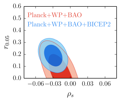
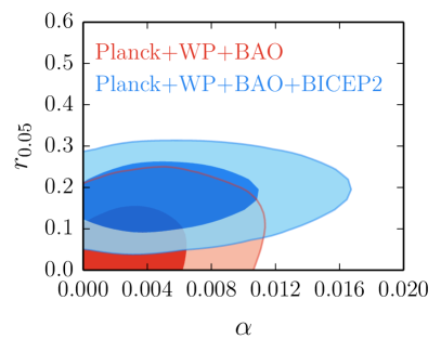
Figure 2: Marginalized 2D posteriors on the tensor-scalar ratio, running, and isocurvature parameters.

We have tested the stability of our results when including the Planck CMB lensing likelihood, removing BAOs, and using ${\cal P}_{h}\propto\bar{k}^{0}$ instead of $\bar{k}^{-r/8}$. We find that the results are relatively robust, although the evidence in favor of running is reduced in some of these cases: the addition of CMB lensing in particular reduces the evidence to $\ln B=1.8$, which is “weak” on Jeffrey’s scale. The Planck collaboration also finds a reduced significance of a running index when using the CMB lensing data Planck Collaboration (2014a).

Our results change more significantly if the same method of Ref. Abazajian et al. (2014) is used, where the posterior likelihood of the tensor-to-scalar ratio obtained by the BICEP2 collaboration was used as a prior instead of calculating the full BICEP2 likelihood for each model. If we use their method, we reproduce their results, which show an even smaller evidence ratio for the running spectral index model, $\ln B=1.1$. While applying the BICEP2 posterior distribution on $r_{0.05}$ as a prior is reasonable when constraining the tensor amplitude only, the results will be only approximately recovered if both $r_{0.05}$ and $\rho_{s}$ are varied simultaneously. This is because the BICEP2 posterior was obtained for a model without running, so that any degeneracy between $r_{0.05}$ and $\rho_{s}$ will be missed if using this approach. We thus conclude that Ref. Abazajian et al. (2014) underestimated the evidence ratio for the running spectral index model.

V Conclusions

There are at least three easy ways to reduce the apparent “tension” between the simplest inflation models with a tensor mode and the current CMB data including Planck and BICEP2. First, a sub-dominant CDM isocurvature perturbation anti-correlated with the dominant curvature perturbation Kawasaki et al. (2014); Bastero-Gil et al. (2014); second, a negative running spectral index BICEP2 Collaboration (2014); and third, a modification of the large-scale primordial power spectrum Abazajian et al. (2014); Bousso et al. (2014); Freivogel et al. (2014); Hazra et al. (2014a, b, c); Meerburg (2014).

We have performed a Bayesian model comparison of the former two extensions against the simplest inflation models. The anti-correlated CDM isocurvature component reduces the CMB temperature power spectrum at low multipoles, improving the agreement with the tensor model with $r_{0.05}=0.2$ suggested by the BICEP2 data without any foreground subtraction. Nonetheless, we have found that such an improvement is Bayesianly disfavored, i.e., the data do not support such an extension of the inflation model, despite that it gives an improved $\chi^{2}$ by $\Delta\chi^{2}=-4.2$. This shows the power of the Bayesian model comparison method. While this result necessarily depends on the chosen prior on the amount of isocurvature, i.e., $\alpha\in[0,1]$, this prior is physically motivated, and there is little room for ambiguity on the prior choice.

We have then tested a model with a running spectral index, as a negative running can also reduce the temperature power spectrum at low multipoles. We have found that a negative running spectral index is moderately favored with the log evidence ratio of $\ln B=2.52$.

Our results are derived assuming that there is no foreground contamination in the BICEP2 data. Any foreground contributions will lower $\ln B$, and thus the anti-correlated CDM isocurvature will be even more disfavored, and the evidence for a negative running spectral index will likely turn to be “weak” ($\ln B<2.5$). The BICEP2 collaboration finds that the polarized dust emission could account for 30% of the measured B-mode power spectrum, while others argue that 100% could be accounted for by dust Mortonson and Seljak (2014); Flauger et al. (2014). Therefore, we conclude that the current data do not require these particular extensions of the simplest inflation models.

References

- Akaike (1974) H. Akaike, IEEE Transactions on Automatic Control 19, 716 (1974).
- Schwarz (1978) G. Schwarz, Annals of Statistics 6, 461 (1978).
- Jeffreys (1961) H. Jeffreys, Theory of Probability, 3rd ed. (Oxford University Press, New York, NY, 1961).
- Trotta (2008) R. Trotta, Contemporary Physics 49, 71 (2008), arXiv:0803.4089 .
- Kolb and Turner (1990) E. W. Kolb and M. S. Turner, The Early Universe (Addison-Wesley, New York, NY, 1990).
- Hinshaw et al. (2013a) G. Hinshaw et al., Astrophys. J. Supp. 208, 19 (2013a), arXiv:1212.5226 [astro-ph.CO] .
- Planck Collaboration (2014a) Planck Collaboration, Astron. Astrophys. 571, A16 (2014a), arXiv:1303.5076 [astro-ph.CO] .
- Lyth and Riotto (1999) D. H. Lyth and A. Riotto, Phys. Rept. 314, 1 (1999).
- Chung et al. (2003) D. J. Chung, G. Shiu, and M. Trodden, Phys. Rev. D 68, 063501 (2003), astro-ph/0305193 .
- Ashoorioon et al. (2014) A. Ashoorioon, K. Dimopoulos, M. M. Sheikh-Jabbari, and G. Shiu, Physics Letters B 737, 98 (2014), arXiv:1403.6099 [hep-th] .
- Planck Collaboration (2014b) Planck Collaboration, Astron. Astrophys. 571, A22 (2014b), arXiv:1303.5082 [astro-ph.CO] .
- Smith et al. (2014) K. M. Smith, C. Dvorkin, L. Boyle, N. Turok, M. Halpern, G. Hinshaw, and B. Gold, Physical Review Letters 113, 031301 (2014), arXiv:1404.0373 .
- BICEP2 Collaboration (2014) BICEP2 Collaboration, Physical Review Letters 112, 241101 (2014), arXiv:1403.3985 .
- Starobinsky (1985) A. A. Starobinsky, Soviet Astronomy Letters 11, 133 (1985).
- Abazajian et al. (2014) K. N. Abazajian, G. Aslanyan, R. Easther, and L. C. Price, J. Cosmol. Astropart. Phys. 8, 053 (2014), arXiv:1403.5922 .
- Hazra et al. (2014a) D. K. Hazra, A. Shafieloo, G. F. Smoot, and A. A. Starobinsky, J. Cosmol. Astropart. Phys. 6, 061 (2014a), arXiv:1403.7786 .
- Hazra et al. (2014b) D. K. Hazra, A. Shafieloo, G. F. Smoot, and A. A. Starobinsky, Physical Review Letters 113, 071301 (2014b), arXiv:1404.0360 .
- Hazra et al. (2014c) D. K. Hazra, A. Shafieloo, G. F. Smoot, and A. A. Starobinsky, J. Cosmol. Astropart. Phys. 8, 048 (2014c), arXiv:1405.2012 .
- Meerburg (2014) P. D. Meerburg, Phys. Rev. D 90, 063529 (2014), arXiv:1406.3243 .
- Kawasaki et al. (2014) M. Kawasaki, T. Sekiguchi, T. Takahashi, and S. Yokoyama, J. Cosmol. Astropart. Phys. 8, 043 (2014), arXiv:1404.2175 .
- Planck Collaboration (2014c) Planck Collaboration, Astron. Astrophys. 571, A15 (2014c), arXiv:1303.5075 .
- Hinshaw et al. (2013b) G. Hinshaw et al., Astrophys. J. Supp. 208, 19 (2013b), arXiv:1212.5226 [astro-ph.CO] .
- Anderson et al. (2012) L. Anderson et al., Mon. Not. R. Astron. Soc. 427, 3435 (2012), arXiv:1203.6594 [astro-ph.CO] .
- Padmanabhan et al. (2012) N. Padmanabhan, X. Xu, D. J. Eisenstein, R. Scalzo, A. J. Cuesta, K. T. Mehta, and E. Kazin, Mon. Not. R. Astron. Soc. 427, 2132 (2012), arXiv:1202.0090 [astro-ph.CO] .
- Beutler et al. (2011) F. Beutler et al., Mon. Not. R. Astron. Soc. 416, 3017 (2011), arXiv:1106.3366 [astro-ph.CO] .
- Feroz et al. (2009) F. Feroz, M. P. Hobson, and M. Bridges, Mon. Not. R. Astron. Soc. 398, 1601 (2009), arXiv:0809.3437 .
- Feroz et al. (2013) F. Feroz, M. P. Hobson, E. Cameron, and A. N. Pettitt, ArXiv e-prints (2013), arXiv:1306.2144 [astro-ph.IM] .
- Lewis et al. (2000) A. Lewis, A. Challinor, and A. Lasenby, Astrophys. J. 538, 473 (2000), arXiv:astro-ph/9911177 .
- Lewis and Bridle (2002) A. Lewis and S. Bridle, Phys. Rev. D 66, 103511 (2002), arXiv:astro-ph/0205436 .
- Bastero-Gil et al. (2014) M. Bastero-Gil, A. Berera, R. O. Ramos, and J. G. Rosa, J. Cosmol. Astropart. Phys. 10, 053 (2014), arXiv:1404.4976 .
- Bousso et al. (2014) R. Bousso, D. Harlow, and L. Senatore, ArXiv e-prints (2014), arXiv:1404.2278 .
- Freivogel et al. (2014) B. Freivogel, M. Kleban, M. Rodriguez Martinez, and L. Susskind, ArXiv e-prints (2014), arXiv:1404.2274 .
- Mortonson and Seljak (2014) M. J. Mortonson and U. Seljak, J. Cosmol. Astropart. Phys. 10, 035 (2014), arXiv:1405.5857 .
- Flauger et al. (2014) R. Flauger, J. C. Hill, and D. N. Spergel, J. Cosmol. Astropart. Phys. 8, 039 (2014), arXiv:1405.7351 .