Phase separation and long wave-length charge instabilities in spin-orbit coupled systems

Abstract

We investigate a two-dimensional electron model with Rashba spin-orbit interaction where the coupling constant $g=g(n)$ depends on the electronic density. It is shown that this dependence may drive the system unstable towards a long-wave length charge density wave (CDW) where the associated second order instability occurs in close vicinity to global phase separation. For very low electron densities the CDW instability is nesting-induced and the modulation follows the Fermi momentum $k_{F}$. At higher density the instability criterion becomes independent of $k_{F}$ and the system may become unstable in a broad momentum range. Finally, upon filling the upper spin-orbit split band, finite momentum instabilities disappear in favor of phase separation alone. We discuss our results with regard to the inhomogeneous phases observed at the LaAlO₃/SrTiO₃ or LaTiO₃/SrTiO₃ interfaces.

I Introduction

The observation of a high-mobility electron gas at the interface of LaAlO₃/SrTiO₃ ohtomo has attracted great interest due to the variety of possibilities of controlling and modifying the properties of a two-dimensional (2D) electron system mannhart08 ; heber09 ; mannhart10 ; hwang12 . Due to the large dielectric constant of the SrTiO₃ substrate, the carrier density and mobility of the 2D electron gas can be tuned by applying a gate voltage either across the substrate caviglia08 ; bell09 or, in a less easy implementation, by depositing the gate on top of the thin upper LaAlO₃ layer. Such electric field effect can be used in order to modulate the electron density and hence the superconductivity reyren ; espci1 . More recently it has been shown by magnetotransport experiments biscaras12 that the electron gas in LaTiO₃/SrTiO₃ heterostructures is composed of two types of carriers, a majority of low mobility carriers that are always present and high-mobility ones which induce superconductivity upon injection with positive gating. In the latter regime, an analysis of the resistivity $R$ has revealed pronounced tails in the $R$ vs. temperature curves caviglia08 ; caprara11 . These tails can be understood with the assumption of an inhomogeneous superconducting order parameter distribution caprara11 ; bucheli13 ; caprara13 . Naturally, the low dimensionality of the electron gas emphasizes the role of disorder which unavoidably is created during the growing process, like, e.g., oxygen vacancies. However, it has been proposed caprara12 ; bucheli132 that the strong Rashba spin-orbit (RSO) interaction may also provide an intrinsic mechanism for the occurrence of electronic phase separation (PS). This point of view is supported by the observation of a negative compressibility li11 in strongly charge depleted LaAlO₃/SrTiO₃ interfaces where the effect seems to go beyond the standard contribution from exchange interactions in a 2D electron gas.

PS together with frustration due to disorder would then be responsible for the formation of mesoscopic superconducting islands embedded in a (weakly localizing) metallic background. The mutual phase coherence between neighboring islands would then generate a low-dimensional percolative superconducting network which is compatible with the observation of ’tailish’ $R(T)$ curves bucheli13 ; caprara13 .

From a formal point of view, the investigation of Ref. caprara12 was restricted to an analysis of the chemical potential vs. electron density, and it was subsequently extended investigating the role of temperature and magnetic field in restoring the homogeneous electronic state bucheli132 . It has been shown that upon increasing the RSO a negative slope corresponding to a PS instability can be induced which is equivalent to a divergence of the density-density response function at zero transferred momentum. Naturally the question arises whether this mechanism is more general and can even lead to finite momentum instabilities. It is exactly this problem which we intend to analyze in the present paper.

In this context it has been shown recently scheurer within a multiband model, that scattering processes between the nested regions of Rashba split subbands may induce a variety of competing phases. In case of a conventional (attractive) pairing these include also charge density waves competing with conventional superconductivity. Here we will demonstrate that charge-density wave instabilities can also be driven by a density-dependent RSO interaction which for the sake of simplicity will be analyzed within a one-band model.

II Model and Formalism

In order to describe the electronic structure of the interface electron gas we consider a 2D lattice model with strong Rashba coupling described by the Hamiltonian evangelou87 ; ando89

$$H = \sum_{ij\sigma}t_{ij}c^{\dagger}_{i\sigma}c_{j\sigma}+\sum_{i}\left[\gamma_{i,i+y}j_{i,i+y}^{x}-\gamma_{i,i+x}j_{i,i+x}^{y}\right]$$ (1)

$$+ \sum_{i,\sigma}\lambda_{i}\left[c^{\dagger}_{i\sigma}c_{i\sigma}-n_{i}\right]$$

with $n_{i}\equiv\sum_{\sigma}\langle c_{i\sigma}^{\dagger}c_{i\sigma}\rangle$. Here, the first term describes the kinetic energy of electrons on a square lattice (with lattice constant $a$) and we only take hopping between nearest-neighbors into account ($t_{ij}\equiv-t$ for $|R_{i}-R_{j}|=a$, and $t_{ij}=0$ otherwise). The second term is the RSO coupling, where

$$j_{i,i+\eta}^{\alpha}=-i\sum_{\sigma\sigma^{\prime}}\left[c^{\dagger}_{i\sigma}\tau^{\alpha}_{\sigma\sigma^{\prime}}c_{i+\eta,\sigma^{\prime}}-c^{\dagger}_{i+\eta,\sigma}\tau^{\alpha}_{\sigma^{\prime}\sigma}c_{i,\sigma}\right]$$ (2)

denotes the $\alpha$-component ($\alpha=x,y,z$) of the spin-current flowing on the bond between $R_{i}$ and $R_{i+\eta}$, and $\tau^{\alpha}$ are the Pauli matrices. The coupling constants obey the relation $\gamma_{ij}=\gamma_{ji}$. The last term in Eq. 1 ensures the local density fixed to $n_{i}$ via the local chemical potential $-\lambda_{i}$ which will become important below when we deal with density-dependent RSO couplings.

Note that for homogeneous coupling constants $\gamma_{i,i+\eta}\equiv\gamma$ the RSO term takes the usual form in momentum space

$$H^{c}=\sum_{\bm{k}\sigma\sigma^{\prime}}\left[\alpha_{\bm{k}}^{x}\tau^{x}_{\sigma\sigma^{\prime}}+\alpha_{\bm{k}}^{y}\tau^{y}_{\sigma\sigma^{\prime}}\right]c_{\bm{k}\sigma}^{\dagger}c_{\bm{k}\sigma}$$ (3)

where ${\bf\alpha}_{\bm{k}}=\gamma(-\frac{\partial\epsilon_{\bm{k}}}{\partial k_{y}},\frac{\partial\epsilon_{\bm{k}}}{\partial k_{x}},0)$ and $\epsilon_{\bm{k}}$ is the 2D lattice dispersion law. Thus a constant $\gamma$ reproduces the customary $(\vec{\bm{v}}\times\vec{\bf\sigma})$ form of the RSO interaction.

The RSO coupling constants depend on the electric field $\bm{E}$ perpendicular to the 2D electron gas. Following Refs. caprara12 and bucheli132 , we argue that the electric field is determined by the charge density in the layer thus yielding a dependence of the RSO coupling constant on the charge density. For the present purpose, it is important to note that this dependency is a local one, i.e., a local charge fluctuation will locally alter the electric field and thus also locally change the RSO coupling constant. We therefore set $\gamma_{i,i+\eta}=\gamma_{i,i+\eta}(n_{i},n_{i+\eta})$ and since by symmetry $\partial\gamma_{i,i+\eta}/\partial n_{i}=\partial\gamma_{i,i+\eta}/\partial n_{i+\eta}$ we consider the following coupling

$$\gamma_{i,i+\eta}=a_{0}+a_{1}(n_{i}+n_{i+\eta}).$$ (4)

Note that in Ref. caprara12 a more general form of the density-dependent coupling has been considered which saturates at large densities. Here we abstain from this extension, in order to keep the number of parameters to a minimum. However, the following instability analysis can be straightforwardly extended to general density-dependent RSO couplings which will induce the formation of electronic inhomogeneities and thus concomitant variations in the local chemical potential. The latter can be obtained self-consistently by minimizing the energy with respect to the local density $\partial E/\partial n_{i}=0$ which yields

$$\lambda_{i}=a_{1}\left(\langle j_{i,i+y}^{x}\rangle-\langle j_{i,i+x}^{y}\rangle\right).$$ (5)

A few words are now in order to account for the introduction of the Lagrange multiplier field $\lambda_{i}$. In general the thermodynamic properties of fermionic systems are more easily calculated in the grand-canonical ensemble, defined by the potential $\Omega=F-\mu N$, where $F$ is the free energy and $N$ the total particle number of the system. In this ensemble the chemical potential is fixed while the particle density (per unit cell) $n=N/L^{2}$ is a fluctuating quantity ($L^{2}$ is the number of lattice sites). Therefore, when we calculate the chemical potential via the density-dependent grand-canonical potential, the density [and therefore also $\gamma(n)$] is not known a priori. An elegant way to circumvent this problem is the introduction of a Lagrange multiplier $\lambda$ as was done in Ref. bucheli132 . In the present non-homogeneous case we proceed similarly and we take the energy to be dependent on a real parameter $n_{i}$, determine the local chemical potential $\mu(\lambda_{i},n_{i})$, and then chose $\lambda_{i}$ to impose $n_{i}=\langle c^{\dagger}_{i\sigma}c_{i\sigma}\rangle$ via Eq. (5).

If we insert the Lagrange parameter Eq. (5) in the Hamiltonian Eq. 1 the energy functional reads as

$$E = E_{0}+a_{1}\sum_{i}\left(n_{i}+n_{i+y}\right)\langle j_{i,i+y}^{x}\rangle$$ (6)

$$- a_{1}\sum_{i}\left(n_{i}+n_{i,i+x}\right)\langle j_{i,i+x}^{y}\rangle$$

with

$$E_{0}=\sum_{ij\sigma}t_{ij}\langle c^{\dagger}_{i\sigma}c_{j\sigma}\rangle+\sum_{i}\left[\gamma^{0}_{i,i+y}\langle j_{i,i+y}^{x}\rangle-\gamma^{0}_{i,i+x}\langle j_{i,i+x}^{y}\rangle\right]$$

and the notation $\gamma^{0}$ refers to the coupling at a given density.

From Eq. (6) it becomes apparent that the density-dependent coupling induces an effective density-current interaction. Assume that the problem has been solved for a given homogeneous density (in the following, we take densities and currents as site independent). Then, one can obtain the instabilities of the system from the expansion of the energy in the small fluctuations of the density matrix in momentum space

$$\delta E = Tr(H\delta\rho)+\frac{a_{1}}{L^{2}}\sum_{\bm{q}}\cos(\frac{q_{y}}{2})\left[\delta\rho_{\bm{q}}\delta j^{x}_{-\bm{q}}+\delta j^{x}_{\bm{q}}\delta\rho_{-{\bm{q}}}\right]$$ (7)

$$- \frac{a_{1}}{L^{2}}\sum_{\bm{q}}\cos(\frac{q_{x}}{2})\left[\delta\rho_{\bm{q}}\delta j^{y}_{-{\bm{q}}}+\delta j^{y}_{\bm{q}}\delta\rho_{-{\bm{q}}}\right].$$

The fluctuations are given by

$$\delta j^{x}_{{\bm{q}}} = -2t\sum_{\bm{k}\sigma\sigma^{\prime}}\sin(k_{y}+\frac{q_{y}}{2})c^{\dagger}_{\bm{k}+\bm{q},\sigma}\tau^{x}_{\sigma\sigma^{\prime}}c_{\bm{k},\sigma^{\prime}}$$

$$\delta j^{y}_{\bm{q}} = -2t\sum_{\bm{k}\sigma\sigma^{\prime}}\sin(k_{x}+\frac{q_{x}}{2})c^{\dagger}_{\bm{k}+\bm{q},\sigma}\tau^{y}_{\sigma\sigma^{\prime}}c_{\bm{k},\sigma^{\prime}}$$

$$\delta\rho_{\bm{q}} = \sum_{\bm{k}\sigma\sigma^{\prime}}c^{\dagger}_{\bm{k}+\bm{q},\sigma}{\bf 1}_{\sigma\sigma^{\prime}}c_{\bm{k},\sigma^{\prime}}\,.$$

and the instabilities can now be determined from a standard random phase approximation (RPA). For this purpose we introduce response functions

$$\chi_{AB}(\bm{q})=-\frac{i}{L^{2}}\int dt\langle{\cal T}\delta A_{\bm{q}}(t)\delta B_{-\bm{q}}(0)\rangle,$$

where $\delta A_{\bm{q}}$ and $\delta B_{\bm{q}}$ refer to the fluctuations defined above.

The non-interacting susceptibilities can be obtained from the eigenstates of the Rashba Hamiltonian Eq. (1). Denoting the response functions in matrix form

$$\underline{\underline{\chi^{0}({\bm{q}})}}=\left(\begin{array}[]{ccc}\chi^{0}_{jx,jx}&\chi^{0}_{jx,jy}&\chi^{0}_{jx,\rho}\\ \chi^{0}_{jy,jx}&\chi^{0}_{jy,jy}&\chi^{0}_{jy,\rho}\\ \chi^{0}_{\rho,jx}&\chi^{0}_{\rho,jy}&\chi^{0}_{\rho,\rho}\end{array}\right)$$ (8)

and the interaction, derived from Eq. (7) as

$$\underline{\underline{V({\bm{q}})}}=\left(\begin{array}[]{ccc}0&0&2\gamma^{\prime}\cos(\frac{q_{y}}{2})\\ 0&0&-2\gamma^{\prime}\cos(\frac{q_{x}}{2})\\ 2\gamma^{\prime}\cos(\frac{q_{y}}{2})&-2\gamma^{\prime}\cos(\frac{q_{x}}{2})&0\end{array}\right)$$ (9)

the full RPA response is given by

$$\underline{\underline{\chi({\bm{q}})}}=\left(\underline{\underline{\bf 1}}-\underline{\underline{\chi^{0}({\bm{q}})}}\underline{\underline{V({\bm{q}})}}\right)^{-1}\underline{\underline{\chi^{0}({\bm{q}})}}.$$ (10)

The instabilities can thus be obtained from the zeros of the determinant $|{\bf 1}-\chi^{0}({\bm{q}})V({\bm{q}})|$.

Here, the element $\chi_{\rho\rho}(\bm{q}=0)$ is proportional to the compressibility, i.e., within our sign convention, proportional to the inverse of $-\partial\mu/\partial n$. A (locally) stable system thus corresponds to $\chi_{\rho\rho}(\bm{q}=0)<0$ whereas an unstable system is characterized by $\chi_{\rho\rho}(\bm{q}=0)>0$. Analogously, a charge density wave (CDW) instability is signalled by a divergence in $\chi_{\rho\rho}(\bm{q}=\bm{Q}_{CDW}\neq 0)$, where $\bm{q}=\bm{Q}_{CDW}$ is the momentum which becomes unstable upon entering the symmetry-broken CDW phase. We also note that a non-linear dependency of the RSO coupling on densities would generate an additional density-density type contribution to the interaction matrix, i.e., $V_{\rho\rho}({\bm{q}})$.

III Long wave-length CDW’s

For the sake of definiteness, in our calculations we fix the constant part of the RSO coupling in Eq. 4 to $a_{0}/t=0.5$. The stability of the system is then analyzed in the $(n;a_{1}/t)$ parameter space where $n$ is the electron density (per unit cell) and $a_{1}/t$ is the component of the RSO interaction which couples to the density [cf. Eq. (4)].

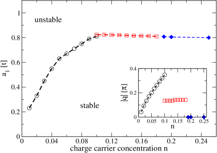
Figure 1: Main panel: Instability line in the $a_{1}/t$ vs. electron density plane with fixed $a_{0}=0.5t$. The range where only the lower RSO-split band is occupied corresponds to the black circles. Above $n=0.105$ both RSO-split bands are occupied (red squares). Both, circles and squares indicate the transition towards a long-wave length CDW whereas diamonds refer to a ${\bf q}=(0,0)$ instability. Inset: Characteristic momentum of the density instability vs. electron density.

Our results are summarized in Fig. 1 which, in the main panel, reports the instability line. Up to $n\approx 0.1$ (circles) it separates a homogenous Fermi liquid from a long-wave length CDW where both $a_{1}/t$ and the CDW modulation $Q_{CDW}$ increase continuously with $n$ (lower right inset). In the range $0.1\lesssim n\lesssim 0.18$ (squares) $Q_{CDW}$ drops discontinuously to a value of $Q_{CDW}\approx 0.14\pi$ and is only weakly density-dependent. Also the slope of the instability line $a_{1}/t$ vs. $n$ decreases only weakly with the electron density. Finally, one enters a PS regime above $n\approx 0.18$ (diamonds) where the unstable momentum discontinuosly jumps to $q=0$ identifying a spinodal line with divergent compressibility. This proximity between the finite-${\bf q}_{c}$ instability and the spinodal line indicates that long-wavelength CDW fluctuations are naturally accompanied by soft density fluctuations at ${\bf q}=(0,0)$ and vice versa.

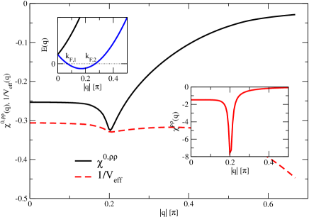
Figure 2: Main panel: Non-interacting susceptibility $\chi^{0}_{\rho\rho}({\bm{q}})$ and inverse effective interaction $1/V_{eff}$ in the low density regime. The lower right inset shows the full density-density response and the upper left inset the bands. Momentum scans are along the $(11)$ direction. Parameters: $n=0.05$, $a_{0}=0.5t$, $a_{1}=0.62t$.

In order to analyze the structure of $\chi_{\rho\rho}({\bm{q}})$ in more detail, it is instructive to define an effective density-density interaction

$$V_{eff}({\bm{q}})=\frac{1}{\chi^{0}_{\rho\rho}({\bm{q}})}-\frac{1}{\chi_{\rho\rho}({\bm{q}})},$$ (11)

which is a function of the non-interacting susceptibility $\chi^{0}_{\rho\rho}({\bm{q}})$ and of the fully dressed $\chi_{\rho\rho}$. According to Eq. (10), this latter includes all the current-current and mixed current-density processes. Therefore $V_{eff}({\bm{q}})$ describes the density-density interaction effectively mediated by all different fluctuations. The correlation function $\chi_{\rho\rho}({\bm{q}})$ is then formally determined from a standard RPA-like expression

$$\chi_{\rho\rho}({\bm{q}})=\frac{\chi^{0}_{\rho\rho}({\bm{q}})}{1-V_{eff}({\bm{q}})\chi^{0}_{\rho\rho}({\bm{q}})}\,.$$ (12)

Fig. 2 reports $\chi^{0}_{\rho\rho}({\bm{q}})$ together with $1/V_{eff}({\bm{q}})$ in the main panel for $n=0.05$. For small momenta, the static density-density correlation function is characterized by a flat part which extends to $2k_{F,1}$ corresponding to scattering between opposite states within the lower RSO-split band (cf. upper inset in Fig. 2). On the other hand, $\chi^{0}_{\rho\rho}({\bf q})$ is strongly enhanced for momenta which connect the two different branches of the Fermi surface of the lower RSO-split band (i.e., $q=k_{F,2}-k_{F,1}$) which drives the instability in this density range. Since we are considering a lattice model small anisotropies in the correlation functions appear already at low density and favor the appearance of the instability along the diagonal $(11)$ direction. The full density-density correlation function, which is reported in the lower right inset to Fig. 2, is then characterized by a sharp peak at $Q_{CDW}$ which shifts to larger momenta with increasing density.

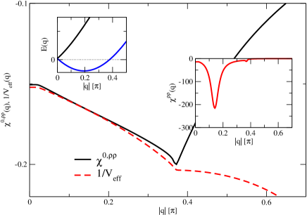
Figure 3: Same as Fig. 2 but for parameters $n=0.12$, $a_{0}=0.5t$, $a_{1}=0.822t$. Momentum scans are along the $(10)$ direction.

Above $n\approx 0.1$ the nesting-induced CDW is replaced by an incommensurate CDW instability at smaller momenta. The situation is analyzed in Fig. 3 for $n=0.12$. Due to the reduced value of $k_{F,1}$ the constant part of $\chi^{0}_{\rho\rho}({\bf q})$ is now limited to small momenta beyond which enhanced interband scattering induces an almost linear increase of the charge density susceptibility. The nesting peak at $q=k_{F,2}-k_{F,1}$ is now much less pronounced since the curvatures of the Fermi surfaces at $k_{F,2}$ and $k_{F,1}$ become more different with increasing density. As a consequence $1/V_{eff}$ touches $\chi^{0}_{\rho\rho}({\bf q})$ in the quasi-linear regime which causes the appearance of a broad peak in the full charge correlation function (right inset to Fig. 3) whereas the nesting peak is only visible as a small feature at $q\sim 0.38\pi$. The unstable momentum hardly changes with $n$ and is located along the vertical (horizontal) direction of the Brillouin zone.

Finally, when the chemical potential enters the upper RSO split band for $n\gtrsim 0.18$, another discontinuous transition occurs towards a $q=0$ instability. The bare charge correlation function $\chi^{0}_{\rho\rho}({\bm{q}})$ (cf. main panel of Fig. 4) has as similar structure than in the previous case (Fig. 3), however, the flat part for small momentum extends now towards twice the Fermi momentum of the upper band $2k_{F,1}$ (cf. lower right inset to Fig. 4). The peak in $\chi^{0}_{\rho\rho}({\bm{q}})$ is determined by interband scattering between Fermi momenta of the RSO split bands and thus occurs at $k_{F,2}-k_{F,1}$. The full charge correlations $\chi_{\rho\rho}({\bm{q}})$ (lower left inset to Fig. 4) still shows an enhancement at the incommensurate momentum $Q_{CDW}\approx 0.2\pi$, however, the divergence is now clearly shifted to $q=0$. As analyzed further below, this instability corresponds to a local maximum which develops in $\mu(n)$ upon increasing $a_{1}$, so that the static compressibility $\kappa=(\partial\mu/\partial n)^{-1}$ diverges.

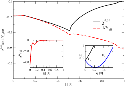
Figure 4: Same as Fig. 2 but for parameters $n=0.19$, $a_{0}=0.5t$, $a_{1}=0.8075t$.

IV Phase separation

The occurrence of electronic PS is locally signaled by the divergence of the compressibility $\kappa=(\partial\mu/\partial n)^{-1}$ marking the spinodal instability line.

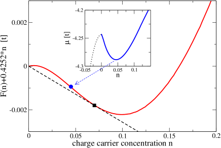
Figure 5: Main panel: Free energy $F(n)$ as a function of electron density (solid). The dashed line reports the Maxwell construction and the point of contact (square) with $F(n)$ indicates the global transition to PS. Inset: Chemical potential as a function of electron density. The minimum, which indicates the local instability point towards PS, corresponds to the point of inflection in $F(n)$ and is indicated by a circle. The dotted line sketches the the behavior in case of a multiband structure as discussed in the text. Parameters: $a_{0}=0.5t$, $a_{1}=0.7t$.

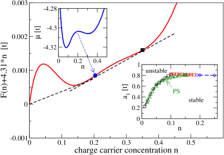
Figure 6: Main panel and upper left inset: Same as Fig. 5 but for larger coupling $a_{1}=0.804t$. The upper right inset shows the PS instability (green triangles) together with the transitions towards CDW order as already reported in Fig. 1.

However, the real PS region is found by implementing the Maxwell construction, which identifies the broader parameter region where the system no longer is formed by a single homogeneous phase. The most natural way to perform the Maxwell construction is by the tangent construction to the free energy, which bypasses the unstable region where the free energy has a wrong concavity, finding a region with lower free energy realized as a linear superposition of two stable phases with different densities. However, to implement this procedure when various phases are present, one should know the free energy of the various phases and refer to the lowest one in each region of the phase diagram. Unfortunately, this program is rather difficult when incommensurate phases are present, which make the calculation of the (meta)stable phases a non-trivial task. Therefore, we will investigate the impact of the Maxwell construction on the phase diagram, by only considering the free energy of the uniform phase. We are aware that at low density the stable phases have an incommensurate CDW order (order parameter $\Delta$), which lowers the free energy by $\sim\Delta^{2}/a_{1}$. This would of course modify the boundaries of the Maxwell construction, which should determine the PS between a uniform phase at high density and a CDW phase at low density.

Nevertheless we find it instructive to perform the Maxwell construction in this approximate way to extract still valuable estimates on the size and structure of the phase separated regions of the phase diagram.

The inset to Fig. 5 reports $\mu(n)$ for $a_{1}=0.7t$ revealing that, for this parameter set and upon lowering the electron density, $\kappa$ diverges at $n\approx 0.05$. However, the global instability towards PS sets in already at larger $n$ and is most conveniently extracted from the tangent construction to the free energy, as exemplified in the main panel of Fig. 5. Upon increasing the coupling $a_{1}$ the corresponding touching points move along the solid line labeled ’PS’ in the lower right inset to Fig. 6.

For completeness, we point out that upon further increasing $a_{1}$ and when the chemical potential has entered the upper RSO-split band, the $\mu$ vs. $n$ curve develops another minimum. At the transition the inflection point with $\partial\mu/\partial n=0$ corresponds to the divergent compressibility and ${\bf q}=0$ instability which is reported by squares in Fig. 1. In this high-density case, the Maxwell construction requires two tangent lines to the free energy which for $a_{1}=0.804t$ are shown in Fig. 6. Coming from large density the system tends to phase separate between $n\approx 0.35$ (cf. squares in Fig. 1) and the other touching point of the tangent at $n\approx 0.18$. This density marks the upper boundary of a tiny stable region which is bound from below by the tangent which connects to $n=0$. The PS line, which is shown in the upper right inset to Fig. 6 together with the instabilites from Fig. 1, does not comprise this situation but is limited to the transition at small $a_{1}$.

V Discussion and Conclusions

Our present investigations reveal the occurence of both PS and long-wavelength charge instabilities in a spin-orbit coupled system where the RSO coupling depends on the electron density (via the confining interface electric field). In particular, we have found that within our model the global transition towards PS is in close vicinity to a second order CDW instability so that PS is accompanied by significant long-wavelength charge fluctuations. Our investigations generalize the analysis of Refs. caprara12 ; bucheli132 , where phases with negative compressibility have been evaluated for a 2D electron gas as realized in oxide heterostructures.

Typically these 2D electron gases are formed at the interfaces between two oxides consisting, respectively, of polar [e.g., (LaO)⁺ and (AlO₂)^-] and non-polar [e.g., TiO₂ and SrO] layers, with typical electron densities (per unit cell) $n\approx 0.01-0.05$. In this regard, a proper description of the electronic states should at least take into account the multiband structure due to the splitting of Ti_3d t_2g bands at the interface. According to the analysis of Refs. caprara12 ; bucheli132 the system is in general stable when the chemical potential falls in the ’light mass’ lower isotropic band of mainly $d_{xy}$ character whereas a PS instability may occur when the gating potential shifts the Fermi energy into the higher anisotropic $d_{xz}$ and $d_{yz}$ bands.

Our present results refer to a model hamiltonian that can be considered as an effective model for these higher energy ’active’ bands. In fact, the RSO coupling used in our analysis compares well with standard values (see. e.g. Ref. bucheli132 ) when the hopping parameter is derived from the dispersion of these ’active’ bands note . The inset to Fig. 5 anticipates then the behavior of the chemical potential (dotted line) in case of an additional ’stable’ lower energy band with $\partial\mu/\partial n>0$. This implies that the lower bound of the phase separated regime as determined by a standard Maxwell construction is no longer at $n=0$ as in our one-band model: The tangent of the Maxwell construction would connect to a density in the ’stable’ lower band. On the other hand, it is conceivable that the implementation of anisotropic ’active’ bands supports the occurence of CDW instabilities which then in Fig. 1 would still be the leading transition at small density.

It would therefore be interesting to explore possible realizations of these instabilities in an ’unrestricted’ multiband model. It might well be that the combination of PS and long-wave length charge instabilities leads to a kind of ’correlated disorder’ which is compatible with the existence of tails in the sheet resistance curves of oxide interfaces below the superconducting transition temperature bucheli13 . Work in this direction is in progress.

- (1) A. Ohtomo and H. Y. Hwang, Nature (London) 427, 423 (2004)
- (2) J. Mannhart, D. H. A. Blank, H. Y. Hwang , A. J. Millis and J. M. Triscone, MRS bulletin 33, 1027 (2008).
- (3) J. Heber, Nature 459, 28 (2009).
- (4) J. Mannhart and D. G. Schlom, Science 327, 1607 (2010).
- (5) H. Y. Hwang et al., Nature Mat. 11, 103 (2012).
- (6) A. D. Caviglia, S. Gariglio, N. Reyren, D. Jaccard, T. Schneider, M. Gabay, S. Thiel, G. Hammerl, J. Mannhart, and J.-M. Triscone1, Nature (London) 456, 624 (2008).
- (7) C. Bell, S. Harashima, Y. Kozuka, M. Kim, B. G. Kim, Y. Hikita, and H. Y. Hwang, Phys. Rev. Lett. 103, 226802 (2009).
- (8) N. Reyren, S. Thiel, A. D. Caviglia, L. Fitting Kourkoutis, G. Hammerl, C. Richter, C. W. Schneider, T. Kopp, A.-S. Retschi, D. Jaccard, M. Gabay, D. A. Muller, J.-M. Triscone, and J. Mannhart, Science 317, 1196 (2007).
- (9) J. Biscaras, N. Bergeal, A. Kushwaha, T. Wolf, A. Rastogi, R. C. Budhani, and J. Lesueur, Nat. Commun., 1, 89 (2010).
- (10) J. Biscaras, N. Bergeal, S. Hurand, C. Grossetete, A. Rastogi, R. C. Budhani, D. LeBoeuf, C. Proust, J. Lesueur, Phys. Rev. Lett. 108, 247004 (2012).
- (11) S. Caprara, M. Grilli, L. Benfatto, and C. Castellani, Phys. Rev. B 84, 014514 (2011).
- (12) D. Bucheli, S. Caprara, C. Castellani, and M. Grilli, New Journal of Physics 15 023014 (2013).
- (13) S. Caprara, J. Biscaras, N. Bergeal, D. Bucheli, S. Hurand, C. Feuillet-Palma, A. Rastogi, R. C. Budhani, J. Lesueur, and M. Grilli, Phys. Rev. B 88, 020504 (2013).
- (14) S. Caprara, F. Peronaci, and M. Grilli, Phys. Rev. Lett. 109, 196401 (2012).
- (15) D. Bucheli, M. Grilli, F. Peronaci, G. Seibold, and S. Caprara, Phys. Rev. B 89, 195448 (2014).
- (16) Lu Li, C. Richter, S. Paetel, T. Kopp, J. Mannhart, R. C. Ashoori, Science 332, 825 (2011).
- (17) M. S. Scheurer and J. Schmalian, arXiv:1404.4039.
- (18) S. N. Evangelou and T. Ziman, J. Phys. C 20, L235 (1987).
- (19) T. Ando, Phys. Rev. B 40, 5325 (1989).
- (20) J. Sinova, D. Culcer, Q. Niu, N. A. Sinitsyn, T. Jungwirth, and A. H. MacDonald, Phys. Rev. Lett. 92, 126603 (2004).
- (21) D. N. Sheng, L. Sheng, Z. Y. Weng, and F. D. M. Haldane, Phys. Rev. B 72, 153307 (2005).
- (22) K. Nomura, J. Sinova, N. A. Sinitsyn, and A. H. MacDonald, Phys. Rev. B 72, 165316 (2005).
- (23) For example, a hopping parameter corresponds to a mass of for the and bands. Taking the lattice parameter for STO this yields a value of for a Rashba coupling of order .