Mixing and Un-mixing by Incompressible Flows

Abstract.

We consider the questions of efficient mixing and un-mixing by incompressible flows which satisfy periodic, no-flow, or no-slip boundary conditions on a square. Under the uniform-in-time constraint $\|\nabla u(\cdot,t)\|_{p}\leq 1$ we show that any function can be mixed to scale $\varepsilon$ in time $O(|\log\varepsilon|^{1+\nu_{p}})$, with $\nu_{p}=0$ for $p<\tfrac{3+\sqrt{5}}{2}$ and $\nu_{p}\leq\tfrac{1}{3}$ for $p\geq\tfrac{3+\sqrt{5}}{2}$. Known lower bounds show that this rate is optimal for $p\in(1,\tfrac{3+\sqrt{5}}{2})$. We also show that any set which is mixed to scale $\varepsilon$ but not much more than that can be un-mixed to a rectangle of the same area (up to a small error) in time $O(|\log\varepsilon|^{2-1/p})$. Both results hold with scale-independent finite times if the constraint on the flow is changed to $\|u(\cdot,t)\|_{\dot{W}^{s,p}}\leq 1$ with some $s<1$. The constants in all our results are independent of the mixed functions and sets.

1. Introduction and Main Results

Mixing of substances by flows and processes involving it are ubiquitous in nature. In the absence of diffusion, or when diffusion acts at time scales much longer than the flow and thus can be neglected in short and medium terms, the basic model for mixing of passive scalars (i.e., with no feedback of the mixed substance on the mixing flow) is the transport equation

$$\rho_{t}+u\cdot\nabla\rho=0,$$ (1.1)

with initial condition $\rho(\cdot,0)=\rho_{0}$. Here $\rho:Q\times{\mathbb{R}}^{+}\to{\mathbb{R}}$ is the mixed scalar (e.g., density of particles of a substance in a liquid), with $Q\subseteq{\mathbb{R}}^{d}$ the physical domain and $\rho_{0}:Q\to{\mathbb{R}}$, while $u:Q\times{\mathbb{R}}^{+}\to{\mathbb{R}}^{d}$ is the mixing flow. Of particular interest in real-world applications are incompressible flows (with $\nabla\cdot u=0$) and questions of their mixing efficiency. A natural (and central) problem in this direction is how well a given initial density $\rho_{0}$ can be mixed by incompressible flows satisfying some physically relevant quantitative constraints.

For the sake of transparency, we will consider here the case of a square $Q=(0,1)^{2}\subseteq{\mathbb{R}}^{2}$, with either the no-flow boundary condition $u\cdot n=0$ on $\partial Q\times{\mathbb{R}}^{+}$ (where $n$ is the unit outer normal to $Q$), or the no-slip boundary condition $u=0$ on $\partial Q\times{\mathbb{R}}^{+}$, or the periodic boundary condition $\rho(0,r,t)=\rho(1,r,t)$ and $\rho(r,0,t)=\rho(r,1,t)$ for all $(r,t)\in(0,1)\times{\mathbb{R}}^{+}$ (when $Q$ becomes the torus ${\mathbb{T}}^{2}$). We will also assume that $\rho_{0}\in L^{\infty}(Q)$ (so $\|\rho(\cdot,t)\|_{\infty}=\|\rho_{0}\|_{\infty}$ for each $t>0$) and is mean-zero on $Q$ (i.e., $\int_{Q}\rho_{0}\,dxdy=0$). Obviously, the latter is not essential since changing $\rho_{0}$ by a constant only changes $\rho$ by the same constant. The restriction to two dimensions is also not essential, as our proofs easily extend to higher dimensions.

To quantify the mixing efficiency of flows, one needs to define a suitable measure of mixing (see, e.g., the review [18]). While in the case of diffusive mixing this may be done in terms of global quantities, such as the decay of $L^{p}$ norms of (a mean-zero) $\rho$ in time [5, 7, 17, 19], solutions of (1.1) have a constant-in-time distribution function, so we need to look at small scale variations of $\rho$ instead. In the present paper we will consider the following natural definition, in which $\fint_{A}fdxdy=|A|^{-1}\int_{A}fdxdy$ is the average of the function $f$ over a set $A$.

Definition 1.1.

Let $f\in L^{\infty}(Q)$ be mean-zero on $Q$ and let $\kappa,\varepsilon\in(0,\tfrac{1}{2}]$. We say that $f$ is $\kappa$-mixed to scale $\varepsilon$ if for each $(x_{0},y_{0})\in Q$,

$$\left|\fint_{B_{\varepsilon}(x_{0},y_{0})\cap Q}f(x,y)dxdy\right|\leq\kappa\|f\|_{\infty}.$$

If now $\rho_{0}\in L^{\infty}(Q)$ is mean-zero, we say that an incompressible flow $u:Q\times{\mathbb{R}}^{+}\to\mathbb{R}^{2}$ $\kappa$-mixes $\rho_{0}$ to scale $\varepsilon$ by time $\tau$ if $\rho(\cdot,\tau)$ is $\kappa$-mixed to scale $\varepsilon$, where $\rho$ solves (1.1) with $\rho(\cdot,0)=\rho_{0}$.

Remark. Another natural definition of mixing that has been used recently is in terms of the $H^{-1}$-norm [1, 8, 10, 9, 15] of $f$. (Other $H^{-s}$ norms [11] or the Wasserstein distance of $f_{+}$ and $f_{-}$ [2, 14, 15, 16] have also been used.) In this case there is no $\kappa$ and the mixing scale is given by $\|f\|_{H^{-1}}\|f\|_{\infty}^{-1}$. We discuss the relation of this definition to Definition 1.1 and our main results after Corollary 1.5 below.

The motivation for Definition 1.1 comes from a paper by Bressan [3], whose definition is a special case of ours. He considered the case $Q={\mathbb{T}}^{2}$ (i.e., periodic boundary conditions), $\kappa=\tfrac{1}{3}$, and $\rho_{0}=\chi_{(0,1/2)\times(0,1)}-\chi_{(1/2,1)\times(0,1)}$, and conjectured that if an incompressible flow $u$ $\tfrac{1}{3}$-mixes $\rho_{0}$ to some scale $\varepsilon\in(0,\tfrac{1}{2}]$ in time $\tau$, then

$$\int_{0}^{\tau}\|\nabla u(\cdot,t)\|_{1}dt\geq C|\log\varepsilon|$$

(with some $\varepsilon$-independent $C<\infty$). Or, equivalently (after an appropriate change of the time variable, as in the proof of Theorems 1.2–1.4 below), that there is $C<\infty$ such that if an incompressible flow $u$ satisfies

$$\sup_{t>0}\|\nabla u(\cdot,t)\|_{1}\leq 1$$ (1.2)

and $\tfrac{1}{3}$-mixes $\rho_{0}$ to some scale $\varepsilon\in(0,\tfrac{1}{2}]$ in time $\tau$, then $\tau\geq C|\log\varepsilon|$. One should think of $\|\nabla u(\cdot,t)\|_{1}$ as an instantaneous cost of the mixing at time $t$, and as we note in Remark 2 after Corollary 1.5 below, the critical order of derivatives of $u$ here is indeed 1.

The above rearrangement cost conjecture of Bressan [3, 4] remains an intriguing open problem. However, its generalized version, with any $\kappa>0$ and (1.2) replaced by

$$\sup_{t>0}\|\nabla u(\cdot,t)\|_{p}\leq 1$$ (1.3)

for some $p\geq 1$ (for $p=2$ this is the bounded enstrophy case), was proved for any $p>1$ by Crippa and De Lellis [6]. Due to a relationship between mixing in the sense of Definition 1.1 and in terms of the $H^{-1}$-norm, discussed after Corollary 1.5, this can be extended to the same result for mixing in the latter sense [8, 15].

Mixing for general functions. Our first goal here is to study the complementary question of how efficient mixing by incompressible flows actually can be, that is, obtaining upper bounds on best possible mixing times by flows satisfying (1.3). We do so by constructing very efficient mixing flows for general mean-zero functions $\rho_{0}\in L^{\infty}(Q)$ and any $\kappa>0$, with any of the three types of boundary conditions. Our main mixing results have $\rho_{0}$-independent bounds and are as follows.

Theorem 1.2.

Consider incompressible flows $u:Q\times{\mathbb{R}}^{+}\to\mathbb{R}^{2}$ satisfying (1.3) for some $p\in[1,\infty]$ and the no-flow boundary condition on $\partial Q\times{\mathbb{R}}^{+}$. For each $p\in[1,\infty]$, there is $C_{p}<\infty$ such that for any mean-zero $\rho_{0}\in L^{\infty}(Q)$ the following holds.

1. If $p\in[1,\tfrac{3+\sqrt{5}}{2})$, then there is $u$ as above which, for any $\kappa,\varepsilon\in(0,\tfrac{1}{2}]$, $\kappa$-mixes $\rho_{0}$ to scale $\varepsilon$ in time $C_{p}|\log(\kappa\varepsilon)|$.

2. If $p=\frac{3+\sqrt{5}}{2}$ ($=\text{golden ratio}+1$), then for any $\kappa\in(0,\tfrac{1}{2}]$ there is $u$ as above which $\kappa$-mixes $\rho_{0}$ to any scale $\varepsilon\in(0,\tfrac{1}{2}]$ in time $C_{p}|\log(\kappa\varepsilon)|\,|\log\frac{|\log(\kappa\varepsilon)|}{\kappa}|^{1/p}$.

3. If $p\in(\frac{3+\sqrt{5}}{2},\infty]$ and $\nu_{p}:=\tfrac{p^{2}-3p+1}{3p^{2}-p}$ (so $\nu_{p}\leq\tfrac{1}{3}$, and $\nu_{\infty}=\tfrac{1}{3}$), then for any $\kappa,\varepsilon\in(0,\tfrac{1}{2}]$, there is $u$ as above which $\kappa$-mixes $\rho_{0}$ to scale $\varepsilon$ in time $C_{p}\kappa^{-\nu_{p}}|\log(\kappa\varepsilon)|^{1+\nu_{p}}$. The flow $u$ can be made independent of $\varepsilon$ if we only require that it $\kappa$-mixes $\rho_{0}$ to scale $\varepsilon$ in time $C_{p}\kappa^{-\nu_{p}}|\log(\kappa\varepsilon)|^{1+\nu_{p}}\log|\log(\kappa\varepsilon)|$.

Theorem 1.3.

Theorem 1.2 continues to hold when the no-flow boundary condition is replaced by the periodic boundary condition.

Theorem 1.4.

Theorem 1.2 continues to hold when the no-flow boundary condition is replaced by the no-slip boundary condition, with the following changes. For $p<\infty$, the term $C_{p}\kappa^{-1+1/p}$ is added to each mixing time (so, in particular, $u$ in (1) also depends on $\kappa$). For $p=\infty$, the mixing times are changed to $C_{p}\kappa^{-1}|\log(\kappa\varepsilon)|^{2}$ for $\varepsilon$-dependent flows and $C_{p}\kappa^{-1}|\log(\kappa\varepsilon)|^{2}(\log|\log(\kappa\varepsilon)|)^{2}$ for $\varepsilon$-independent flows.

Remarks. 1. Of particular interest is the $\varepsilon$-dependence of the mixing times, for a fixed $\kappa>0$ [3, 4, 6]. Due to the abovementioned result from [6], our $O(|\log\varepsilon|)$ upper bound on the shortest mixing time is exact for $p\in(1,\tfrac{3+\sqrt{5}}{2})$. We do not know whether our bound for $p\geq\tfrac{3+\sqrt{5}}{2}$ is optimal for general $\rho_{0}$, or whether the value $p=\tfrac{3+\sqrt{5}}{2}$ is indeed critical here.

2. Since the flow in Theorems 1.2(1) and 1.3(1) is independent of both $\varepsilon$ and $\kappa$, taking $\kappa=\varepsilon$ yields $\varepsilon$-mixing in time $O(|\log\varepsilon|)$ for each $\varepsilon$. In the special case of periodic boundary conditions, initial value $\rho_{0}=\chi_{(0,1/2)\times(0,1)}-\chi_{(1/2,1)\times(0,1)}$, and (1.3) replaced by $\sup_{t>0}\|u(\cdot,t)\|_{\dot{BV}}\leq 1$, an $O(|\log\varepsilon|)$ upper bound was previously obtained in [4, 10].

3. The jump in the power of $|\log(\kappa\varepsilon)|$ at $p=\infty$ in Theorem 1.4 is due to the no-slip condition having an exponentially decreasing effect (at the rate $2^{-n/p}$) for $p<\infty$ as our flow acquires progressively smaller scales (of size $2^{-n}$, with $n\lesssim|\log(\kappa\varepsilon)|$). This is then controlled by other terms in the relevant estimates. For $p=\infty$ this effect stays large at all scales and becomes the dominant term. The details are in the proofs of Theorems 5.4 and 5.3.

4. It is easy to see that if $\rho_{0}$ is supported away from $\partial Q$, then the bounds from Theorem 1.2 also hold in Theorem 1.4, albeit with $C_{p}$ also depending on $\operatorname*{dist}(\text{\rm{supp}}\,\rho_{0},\partial Q)$.

Proofs.

Theorem 1.2 is equivalent to Theorems 3.4, 4.5, and 4.6; Theorem 1.3 is equivalent to Theorem 5.1; and Theorem 1.4 is equivalent to Theorems 5.2, 5.3, and 5.4. The equivalences are obtained by noticing that if $J(t):=\int_{0}^{t}\|\nabla u(\cdot,s)\|_{p}\,ds$, then the solution $\tilde{\rho}$ of (1.1) with the flow $\tilde{u}(\cdot,J(t)):=\|\nabla u(\cdot,t)\|_{p}^{-1}u(\cdot,t)$ (and $\tilde{\rho}(\cdot,0)=\rho_{0}$) satisfies $\tilde{\rho}(\cdot,J(t))=\rho(\cdot,t)$. ∎

Remark. The flows in this paper will all be piece-wise constant (and hence discontinuous) in time (including the rescaled flow in the above proof). However, continuity or smoothness in time is easily obtained by a change of the time variable on each interval on which the flow is constant. For instance, if $u(\cdot,t)=u_{0}(\cdot)$ for $t\in[t_{0},t_{1}]$, we may take $\tilde{u}(\cdot,t):=\alpha(t)u_{0}(\cdot)$ for $t\in[t_{0},t_{1}]$ and some $\alpha\in C_{c}^{\infty}([t_{0},t_{1}])$ with $\int_{t_{0}}^{t_{1}}\alpha(t)dt=t_{1}-t_{0}$. Indeed, if $\tilde{\rho}$ solves (1.1) with $\tilde{u}$ in place of $u$ and $\tilde{\rho}(\cdot,0)=\rho(\cdot,0)$, then $\tilde{\rho}(\cdot,t)=\rho(\cdot,t_{0}+\int_{t_{0}}^{t}\alpha(s)ds)$ for all $t\in[t_{0},t_{1}]$.

A natural question is what happens if $\|\nabla u(\cdot,t)\|_{p}$ is replaced by $\|u(\cdot,t)\|_{\dot{W}^{s,p}}$ in (1.3). The flows we construct throughout this paper have a “self-similar” nature — they are “turbulent” at an exponentially decreasing sequence of scales as time progresses — that allows us to answer this question rather easily. Let us consider the family of squares (cells)

$$Q_{nij}:=\left(\frac{i}{2^{n}},\frac{i+1}{2^{n}}\right)\times\left(\frac{j}{2^{n}},\frac{j+1}{2^{n}}\right),$$

with $n\geq 0$ and $i,j\in\{0,\ldots,2^{n}-1\}$. (Note that $\{Q_{nij}\}_{i,j=0}^{2^{n}-1}$ tile $Q$ for each fixed $n$.) Let us also consider only the $\varepsilon$-independent flows from Theorems 1.2–1.4, before the rescaling from the above proof, that is, as in the proofs of the theorems mentioned there. Those proofs show that for each such flow $u$ and each $n\geq 0$ we have that $u|_{(n,n+1]}$ keeps all the $Q_{nij}$ invariant (“self-similarity”) and for some $C_{p}^{\prime}<\infty$ we have either

$$\sup_{t\in(n,n+1]}\|\nabla u(\cdot,t)\|_{p}\leq C_{p}^{\prime}\qquad\text{and}\qquad\sup_{t\in(n,n+1]}\|u(\cdot,t)\|_{\infty}\leq C_{p}^{\prime}2^{-n}$$

in Theorems 1.2(1) and 1.3(1), or or the same with extra factors $\kappa^{-1}n(\log n)^{2}$ on the right-hand sides in the other cases (these latter worst case bounds are achieved for $p=\infty$ in Theorem 1.4). The interpolation inequality $\|u\|_{\dot{W}^{s,p/s}}\leq C_{s,p}\|\nabla u\|_{p}^{s}\|u\|_{\infty}^{1-s}$ for $s\in[0,1]$ (see, e.g., [12, p. 536]) now yields either

$$\sup_{t\in(n,n+1]}\|u(\cdot,t)\|_{\dot{W}^{s,p/s}}\leq C_{s,p}^{\prime}2^{-(1-s)n}$$

in Theorems 1.2(1) and 1.3(1), or the same with an extra factor $\kappa^{-1}n(\log n)^{2}$ on the right-hand side in the other cases. Then the rescaling in time from the above proof (but corresponding to the $\dot{W}^{s,p/s}$-norm) provides a flow that is uniformly bounded in time in $\dot{W}^{s,p/s}(Q)$ and $\kappa$-mixes $\rho_{0}$ to scale 0 in finite time $\tau$ (in the sense that for each $\varepsilon>0$ there is $\tau_{\varepsilon}<\tau$ such that $\rho(\cdot,t)$ is $\kappa$-mixed to scale $\varepsilon$ for each $t\in(\tau_{\varepsilon},\tau)$). This yields the following.

Corollary 1.5.

Consider incompressible flows $u:Q\times(0,\tau)\to\mathbb{R}^{2}$ satisfying

$$\sup_{t\in(0,\tau)}\|u(\cdot,t)\|_{\dot{W}^{s,p}}\leq 1$$

for some $p\in[1,\infty]$ and $s\in[0,1)$, any one of the three boundary conditions above on $\partial Q\times{\mathbb{R}}^{+}$, and also $\sup_{t\in(0,\tau-\delta)}\|\nabla u(\cdot,t)\|_{\max\{sp,1\}}<\infty$ for each $\delta>0$.

1. If $s<\tfrac{3+\sqrt{5}}{2p}$ and the boundary condition is no-flow or periodic, then there is $\tau_{s,p}<\infty$ such that for any mean-zero $\rho_{0}\in L^{\infty}(Q)$ there is $u$ as above with $\tau:=\tau_{s,p}$ which, for any $\kappa\in(0,\tfrac{1}{2}]$, $\kappa$-mixes $\rho_{0}$ to scale 0 in time $\tau_{s,p}$.

2. If either $s\geq\frac{3+\sqrt{5}}{2p}$ or the boundary condition is no-slip, then for any $\kappa\in(0,\tfrac{1}{2}]$ there is $\tau_{s,p,\kappa}<\infty$ such that for any mean-zero $\rho_{0}\in L^{\infty}(Q)$ there is $u$ as above with $\tau:=\tau_{s,p,\kappa}$ which $\kappa$-mixes $\rho_{0}$ to scale 0 in time $\tau_{s,p,\kappa}$.

Remarks. 1. One can use the above argument to also show algebraic-in-$\varepsilon$ time of $\kappa$-mixing of $\rho_{0}$ for $s>1$, but one needs to adjust our flows appropriately near the boundaries of the $Q_{nij}$ to make them belong to $\dot{W}^{s,p}(Q)$ in this case. We leave the details to the reader.

2. The above suggests that 1 is indeed the critical order of derivatives of $u$ in (1.3).

3. It is not difficult to show that this result, and the fact that $u|_{(n,n+1]}$ before the above rescaling keeps all the $Q_{nij}$ invariant, show that $\rho$ weak-$*$ converges in $L^{\infty}(Q)$ to 0 in (1) and to a function with values in $[-\kappa,\kappa]$ in (2) as $t\to\tau$.

As we mentioned in the remark after Definition 1.1, another measure of the mixing scale of a mean-zero $f\in L^{\infty}(Q)$ is $\|f\|_{H^{-1}}\|f\|_{\infty}^{-1}$. One can easily check that $f$ being $\kappa$-mixed to scale $\varepsilon$ implies that the mix-norm of $f$ [11] is bounded above by $C\sqrt{\varepsilon+\kappa^{2}}\|f\|_{\infty}$ for some $C<\infty$ [11, (8)–(10)]. Hence from the equivalence between the mix-norm and the $H^{-1/2}$ norm [11, Corollary 2.1] one immediately has $\|f\|_{H^{-s}}\leq C\sqrt{\varepsilon+\kappa^{2}}\|f\|_{\infty}$ for all $s\geq\tfrac{1}{2}$.

On the other hand, Lemma A.1 shows that $\|f\|_{H^{-1}}\leq c\kappa^{3/2}\varepsilon^{2}\|f\|_{\infty}$ (with some $c>0$) implies that $f$ is $\kappa$-mixed to scale $\varepsilon$. This, combined with the result from [6], immediately shows that there is $c_{p}>0$ such that if $\rho_{0}=\chi_{(0,1/2)\times(0,1)}-\chi_{(1/2,1)\times(0,1)}$ and an incompressible flow $u$ satisfies (1.3) for some $p\in(1,\infty]$, then $\|\rho(\cdot,\tau)\|_{H^{-1}}\leq\varepsilon\|\rho_{0}\|_{\infty}$ implies $\tau\geq c_{p}|\log\varepsilon|$ (this is also proved in [8, 15]). One may again ask whether this $O(|\log\varepsilon|)$ bound is achievable.

Parts (1) of Theorems 1.2–1.4 (and $\|f\|_{H^{-1}}\leq C\sqrt{\varepsilon}\|f\|_{\infty}$ above when $\kappa:=\varepsilon$) show that there indeed is $C_{p}<\infty$ such that for any mean-zero $\rho_{0}\in L^{\infty}(Q)$ there is an incompressible flow $u$ satisfying (1.3) which yields $\|\rho(\cdot,\tau)\|_{H^{-1}}\leq\varepsilon\|\rho_{0}\|_{\infty}$ for some $\tau\leq C_{p}|\log\varepsilon|$, albeit only for $p\in[1,\tfrac{3+\sqrt{5}}{2})$ in the case of no-flow and periodic boundary conditions (which includes the uniformly bounded enstrophy case, (1.3) with $p=2$), and for $p=1$ in the case of no-slip boundary conditions. (This obviously also yields a corresponding extension of Corollary 1.5.). The difference is that for these $p$ we achieve “perfect” mixing, with $\int_{Q_{nij}}\rho(x,y,t)dxdy=0$ for any $t\geq n$ and $i,j\in\{0,\cdots,2^{n}-1\}$, so $\kappa$ plays a less prominent role in the obtained bounds. We are not able to do this in the other cases and, ironically, it turns out that the enemy to this effort is the possibility of $\rho(\cdot,n)$ being very well mixed inside some $Q_{nij}$ (but not near its boundary). Unfortunately, we cannot discard this possibility for general $\rho_{0}$.

A few days before we finished writing the present paper, Alberti, Crippa, and Mazzucato [1] announced that in the case of periodic boundary conditions they are able to obtain the above $O(|\log\varepsilon|)$ bound (i.e., $\|\rho(\cdot,\tau)\|_{H^{-1}}\leq\varepsilon\|\rho_{0}\|_{\infty}$ with $\tau\leq C_{p}|\log\varepsilon|$) for $\rho_{0}=\chi_{(0,1/2)\times(0,1)}-\chi_{(1/2,1)\times(0,1)}$ and any $p\in[1,\infty]$. For $p\in[1,\infty)$ they can prove the same result with $\rho_{0}$ being the characteristic function of any $A\subseteq{\mathbb{T}}^{2}$ with a smooth boundary and finitely many connected components (minus a constant to make $\rho_{0}$ mean-zero), albeit with the constant $C_{p}$ also depending on $A$. Their method has a more geometric flavor than ours, but is also centered around flows with a “self-similar” structure, and they are able to obtain a better control of $\rho(\cdot,n)$ inside the cells $Q_{nij}$ for these special initial data and the flows they construct. A paper with the proofs of the results announced in [1] will appear later.

Un-mixing for general sets. Our second goal, closely related to the first, concerns the question of efficient un-mixing by incompressible flows. Here it is natural to consider (measurable) sets $A\subseteq Q$ and ask how efficiently can they be transported by incompressible flows close to their un-mixed states $\tilde{A}:=(0,|A|)\times(0,1)$. Or, equivalently (after time-reversal), how efficiently can the rectangle $\tilde{A}$ be transported close to a desired set $A$ of the same measure, instead of just being mixed. Hence, this is a more delicate question than that of mixing, albeit restricted to initial data which are characteristic functions of sets. We are not aware of previous work in this direction. The somewhat related but quite different phenomenon of coarsening has been studied before (e.g., in [2, 14, 16]).

Obviously, the time of un-mixing, given the constraint (1.3), will depend on the scale to which $A$ is mixed. By this we mean the scale $\varepsilon=2^{-n}$ such that most of the squares $Q_{nij}$ are each mostly contained in $A$ or in $Q\setminus A$. Since this scale is given, it makes little sense to ask whether the constructed flows can be $\varepsilon$-independent. We will therefore drop (1.3), require the un-mixing to happen in time 1, and try to minimize $\sup_{t\in(0,1]}\|\nabla u(\cdot,t)\|_{p}$ instead. This is an equivalent question, due to rescaling in time, and will allow our flows to be $p$-independent.

Our main un-mixing result, illustrated in Figure 1, is now as follows (with the no-slip boundary condition, so the other two hold as well).

Theorem 1.6.

There is $C>0$ such that for any measurable $A\subseteq Q$, $n\geq 0$, and $\kappa\in(0,\tfrac{1}{2}]$, the following holds. If at most $2^{2n}\kappa$ of the squares $\{Q_{nij}\}_{i,j=0}^{2^{n}-1}$ satisfy $2^{2n}|A\cap Q_{nij}|\in(\kappa,1-\kappa)$, then there is an incompressible flow $u:Q\times(0,1)\to\mathbb{R}^{2}$ with $u=0$ on $\partial Q\times(0,1)$ and

$$\sup_{t\in(0,1)}\|\nabla u(\cdot,t)\|_{p}\leq C\kappa^{-1+1/p}n^{2-1/p}\qquad\text{for each $p\in[1,\infty]$}$$ (1.4)

such that if $\rho$ solves (1.1) and $\rho(\cdot,0)=\chi_{A}$, then the set $B$ for which $\rho(\cdot,1)=\chi_{B}$ satisfies

$$\left|B\cap\left[(0,|A|)\times(0,1)\right]\right|\geq 1-2\kappa.$$

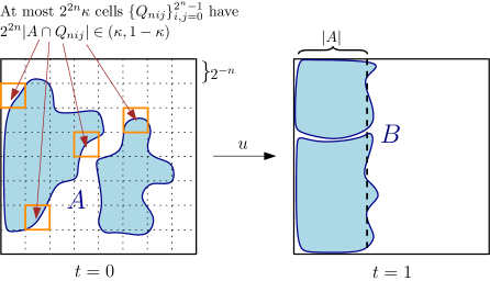
Figure 1. An illustration of un-mixing from Theorem 1.6.

Remarks. 1. By $\rho$ solving (1.1) we mean that $\rho(\cdot,t):=\chi_{S(t)}$, with $S(t):=\{X_{(x,y)}(t)\,:\,(x,y)\in A\}$ and $X_{(x,y)}$ solving $X_{(x,y)}^{\prime}(t)=u(X_{(x,y)}(t),t)$ and $X_{(x,y)}(0)=(x,y)$.

2. When (1.4) is replaced by $\sup_{t\in(0,1)}\|u(\cdot,t)\|_{\dot{BV}}\leq Cn$, this also holds for $\kappa=0$ and the no-flow boundary condition $u\cdot n=0$ on $\partial Q\times(0,1)$ (see the end of the proof).

3. Scaling of $u$ in time (which is different for different $p$) shows that if we require $\sup_{t\in(0,\tau)}\|\nabla u(\cdot,t)\|_{p}\leq 1$, then the time $\tau$ of the above un-mixing satisfies $\tau\leq C\kappa^{-1+1/p}n^{2-1/p}$. That is, if $A$ is mixed to scale $\varepsilon$ but not much more than that (in the sense of Theorem 1.6), it can be unmixed in time $O(|\log\varepsilon|^{2-1/p})$.

4. Similarly to the case of mixing, the “self-similar” structure of the flows we construct shows that Theorem 1.6 holds with (1.4) replaced by $\sup_{t\in(0,1)}\|u(\cdot,t)\|_{\dot{W}^{s,p}}\leq C_{s,p,\kappa}$ when $s\in[0,1)$ (i.e., the bound is independent of the scale $2^{-n}$). Notice that for any $\kappa>0$, any measurable set $A\subseteq Q$ satisfies the hypotheses of the theorem for all large enough $n$.

Finally, here is an interesting corollary of our construction of un-mixing flows, related to the last remark. It shows that for $s<\tfrac{1}{p}$, a rectangle can be transformed into any measurable set of the same measure in finite time by an incompressible flow which is uniformly in time bounded in $\dot{W}^{s,p}(Q)$ and satisfies the no-flow boundary condition (it also has bounded variation, so that (1.1) is well-posed). Notice that there are no errors and no $\kappa$ here.

Corollary 1.7.

For any $s<\tfrac{1}{p}$ there is $C_{s,p}<\infty$ such that for any measurable $A\subseteq Q$ there is an incompressible flow $u:Q\times(0,1)\to\mathbb{R}^{2}$ with $u\cdot n=0$ on $\partial Q\times(0,1)$, satisfying $\sup_{t\in(0,1-\delta)}\|u(\cdot,t)\|_{BV}<\infty$ for any $\delta>0$ and

$$\sup_{t\in(0,1)}\|u(\cdot,t)\|_{\dot{W}^{s,p}}\leq C_{s,p},$$ (1.5)

such that if $\rho$ solves (1.1) and $\rho(\cdot,0)=\chi_{\{0<x<|A|\}}$, then $\lim_{t\to 1}\|\rho(\cdot,t)-\chi_{A}\|_{1}=0$.

Organization of the paper. Theorem 1.2(1) is proved in Sections 2 and 3, and its parts (2) and (3) are proved in Section 4. Section 2 contains the simplest version of our method of construction of mixing flows, which only works for $p<2$. The cases $p\in[2,\tfrac{3+\sqrt{5}}{2})$ and $p\in[\tfrac{3+\sqrt{5}}{2},\infty]$, treated in Sections 3 and 4, are progressively more complicated. However, in a remark at the beginning of Section 4 we provide for the convenience of the reader a relatively simple extension of the argument from Section 2 which treats all $p\in[1,\infty]$ (as well as other boundary conditions), although the bounds obtained are worse than in Theorems 1.2–1.4.

The proofs of Theorems 1.3 and 1.4 appear in Section 5. The un-mixing results are then proved in Section 6, which only uses results from Section 2 (it is also closely related to the abovementioned remark in Section 4). Some technical lemmas are left for the Appendix.

Acknowledgements. The authors wish to thank Inwon Kim, Alexander Kiselev, Andreas Seeger, Brian Street, and Jean-Luc Thiffeault for stimulating discussions. YY acknowledges partial support by NSF grants DMS-1104415, DMS-1159133 and DMS-1411857. AZ acknowledges partial support by NSF grants DMS-1056327 and DMS-1159133.

2. Perfect mixing for no-flow boundary conditions and $p<2$

In this section, we will start with the simplest case, $p<2$ (plus the no-flow boundary condition $u\cdot n=0$ on $\partial Q$), and show that the lower bound $C_{p,\kappa}|\log\varepsilon|$ on the mixing time obtained by Crippa and De Lellis [6] is in fact attainable for these $p$. In the next section we will extend this result to all $p<\tfrac{3+\sqrt{5}}{2}$. We note that the flows we construct in this and the next section will in fact yield $\int_{Q_{nij}}\rho(x,y,t)dxdy=0$ for any $t\geq n$ and $i,j\in\{0,\cdots,2^{n}-1\}.$ This is what “perfect mixing” in the sections’ titles refers to.

We start with the construction of two stream functions $\psi$ and $\eta$, which will serve as the basic building blocks for the subsequent construction of our flow $u$.

Construction of the stream functions. Let $\bar{Q}_{c}:=[0,1]^{2}\setminus\{(0,0),(0,1),(1,0),(1,1)\}$ be the closed square without the corners and let $\partial Q_{c}:=\partial Q\cap\bar{Q}_{c}$ be its boundary without the corners. For a stream function $\psi\in C(Q)$, denote $\nabla\psi:=(\psi_{x},\psi_{y})$ and $\nabla^{2}\psi:=(\psi_{xx},\psi_{xy},\psi_{yx},\psi_{yy})$. If the level set $\{\psi=s\}$ is a simple closed curve, we define

$$T_{\psi}(s):=\int_{\{\psi=s\}}\frac{1}{|\nabla\psi|}d\sigma.$$

Notice that then $T_{\psi}(s)$ equals the time a particle advected by the (incompressible) flow

$$u=\nabla^{\perp}\psi:=(-\psi_{y},\psi_{x})$$

traverses the curve $\{\psi=s\}$. If the level set is a point, we let $T_{\psi}(s):=\lim_{s^{\prime}\to s}T_{\psi}(s^{\prime})$, provided the (one-sided) limit exists.

Proposition 2.1.

There exists a stream function $\psi\in C(\bar{Q})$, with $\nabla\psi$ continuous on $\bar{Q}_{c}$ and differentiable on $Q\setminus\{(\tfrac{1}{2},\tfrac{1}{2})\}$, such that:

1. $\psi>0$ on Q, $\psi=0$ on $\partial Q$, $\nabla\psi\in L^{\infty}(Q)$, and $\partial_{n}\psi=-4$ on $\partial Q_{c}$;

2. $\nabla^{2}\psi\in L^{p}(Q)$ for all $p\in[1,2)$;

3. the level set $\{\psi=s\}$ for each $s\in[0,\|\psi\|_{\infty})$ is a simple closed curve and for $s=\|\psi\|_{\infty}$ it is the point $(\tfrac{1}{2},\tfrac{1}{2})$, and $T_{\psi}(s)=1$ for each $s\in[0,\|\psi\|_{\infty}]$.

We will obtain $\psi$ by modifying the stream function $\varphi$ from the following lemma, which satisfies (1) and (2), but not (3). The proof of the lemma is elementary but a little tedious, so we postpone it to the appendix.

Lemma 2.2.

The function

$$\varphi(x,y):=\frac{4}{\pi}\,\frac{\sin(\pi x)\sin(\pi y)}{\sin(\pi x)+\sin(\pi y)}$$ (2.1)

on $\bar{Q}$ (defined to be 0 in the four corners) satisfies:

1. $\varphi>0$ on Q, $\varphi=0$ on $\partial Q$, $\nabla\varphi\in L^{\infty}(Q)$ and $\partial_{n}\varphi=-4$ on $\partial Q_{c}$;

2. $\nabla^{2}\varphi\in L^{p}(Q)$ for all $p\in[1,2)$;

3. the level set $\{\varphi=s\}$ for each $s\in[0,\tfrac{2}{\pi})$ is a simple closed curve and for $s=\tfrac{2}{\pi}$ it is the point $(\tfrac{1}{2},\tfrac{1}{2})$, and $\sup_{s\in[0,2/\pi]}T_{\varphi}(s)<\infty$ and $T_{\varphi}(0)=1$;

4. $T_{\varphi}$ is differentiable on $(0,\tfrac{2}{\pi})$ and $\sup_{s\in(0,2/\pi)}|\log s|^{-1}|T_{\varphi}^{\prime}(s)|\sup_{\{\varphi=s\}}|\nabla\varphi|^{2}<\infty$.

Proof of Proposition 2.1.

With $\varphi$ from Lemma 2.2, we let

$$\psi(x,y):=\int_{0}^{\varphi(x,y)}T_{\varphi}(s)ds,$$ (2.2)

so that $\varphi$ and $\psi$ share their level sets (although their values are different) and

$$\nabla\psi(x,y)=T_{\varphi}(\varphi(x,y))\nabla\varphi(x,y).$$ (2.3)

The properties of $\nabla\psi$ and (1) now follow from the definition of $\varphi$ and Lemma 2.2(1,3). Since from (2.3) we have

$$|\nabla^{2}\psi|\leq|\nabla^{2}\varphi|\,T_{\varphi}(\varphi(x,y))+|\nabla\varphi|^{2}\left|T^{\prime}_{\varphi}(\varphi(x,y))\right|,$$ (2.4)

(2) holds due to (for some $C<\infty$)

$$\begin{split}\frac{1}{C}\int_{Q}\left(|\nabla\varphi|^{2}\left|T^{\prime}_{\varphi}(\varphi)\right|\right)^{p}dxdy&\leq\int_{Q}\left|\log\varphi\right|^{2}dxdy\qquad\text{(by $p<2$ and Lemma \ref{lemma:phi}(4))}\\ &=\int_{0}^{2/\pi}|\log s|^{2}\int_{\{\varphi=s\}}\frac{1}{|\nabla\varphi|}d\sigma ds\qquad\text{(by the co-area formula)}\\ &=\int_{0}^{2/\pi}|\log s|^{2}T_{\varphi}(s)ds<\infty\qquad\text{(by Lemma \ref{lemma:phi}(3))}.\end{split}$$

Finally, if $F(s):=\int_{0}^{s}T_{\varphi}(s^{\prime})ds^{\prime}$ (and $F^{-1}$ is its inverse function), then Lemma 2.2(3) and

$$T_{\psi}(s)=\int_{\{\psi=s\}}\frac{1}{|\nabla\psi(s)|}ds=\int_{\{\varphi=F^{-1}(s)\}}\frac{1}{|\nabla\varphi|\,T_{\varphi}(F^{-1}(s))}d\sigma=1$$

yield (3). ∎

Let $\bar{Q}_{cc}:=\bar{Q}_{c}\setminus\{(\tfrac{1}{2},0),(\tfrac{1}{2},1),(0,\tfrac{1}{2}),(1,\tfrac{1}{2}),(\tfrac{1}{2},\tfrac{1}{2})\}$ be $\bar{Q}$ without the 9 corners and centers of $Q$ and its sides, and let $\partial Q_{cc}:=\partial Q\cap\bar{Q}_{cc}$. Besides $\psi$ from Proposition 2.1, we will need the following stream function $\eta$ (which satisfies $\nabla\eta=\nabla\psi$ on $\partial Q_{cc}$).

Proposition 2.3.

There exists a stream function $\eta\in C(\bar{Q})$, with $\nabla\eta$ continuous on $\bar{Q}_{cc}$ and differentiable on $Q\setminus\left(\{x=\tfrac{1}{2}\}\cup\{y=\tfrac{1}{2}\}\cup\{x+y=\tfrac{1}{2}\}\cup\{x+y=\tfrac{3}{2}\}\right)$, such that:

1. $\eta=0$ on $\partial Q\cup\{x=\tfrac{1}{2}\}\cup\{y=\tfrac{1}{2}\}$, $\nabla\eta\in L^{\infty}(Q)$, and $\partial_{n}\eta=-4$ on $\partial Q_{cc}$;

2. $\nabla^{2}\eta\in L^{p}(Q)$ for all $p\in[1,2)$.

Proof.

Decompose $Q$ into two squares and four triangles, separated by the lines $\{x=\tfrac{1}{2}\}$, $\{y=\tfrac{1}{2}\}$, $\{x+y=\tfrac{1}{2}\}$, $\{x+y=\tfrac{3}{2}\}$ (see Figure 2). On the two squares $Q_{3}$ and $Q_{4}$, we let $\eta(x,y)=\frac{1}{2}\psi(2(x-x_{0}),2(y-y_{0}))$, where $\psi$ is from Proposition 2.1, and $(x_{0},y_{0})$ is the lower left corner of $Q_{3}$ and $Q_{4}$, respectively.

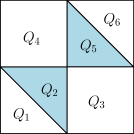
Figure 2. The decomposition of $Q$ from the construction of $\eta$.

On $Q_{1}$ we let

$$\eta(x,y)=4\left(\frac{1}{x}+\frac{1}{y}+\frac{\sqrt{2}}{\frac{1}{2}-x-y}\right)^{-1}.$$ (2.5)

One can easily check that $\eta=0$ on $\partial Q_{1}$ and $\partial_{n}\eta=-4$ on $\partial Q_{1}$ (except at the corners). Differentiation yields $\nabla\eta\in L^{\infty}(Q_{1})$ and $d\nabla^{2}\eta\in L^{\infty}(Q_{1})$, where the function $d$ is the distance from the closest corner of $Q_{1}$. It follows that $\nabla^{2}\eta\in L^{p}(Q_{1})$ for all $p\in[1,2)$.

Finally, in $Q_{2}$ we define $\eta$ by odd reflection across $\{x+y=\tfrac{1}{2}\}$ from $Q_{1}$ (in particular, $\nabla\eta$ is then continuous on $\partial Q_{2}$), and in $Q_{5}\cup Q_{6}$ by even reflection across $\{x+y=1\}$ from $Q_{1}\cup Q_{2}$. The desired properties of $\eta$ on $Q$ then follow immediately from the above properties of $\eta$ on $Q_{1}$ and the properties of $\psi$. Note also that $\eta>0$ on $Q_{1}\cup Q_{3}\cup Q_{4}\cup Q_{6}$ (white in Figure 2) and $\eta<0$ on $Q_{2}\cup Q_{5}$ (blue in Figure 2). ∎

Construction of the mixing flows. We are now ready to prove our first mixing result.

Theorem 2.4.

For any mean-zero $\rho_{0}\in L^{\infty}(Q)$, there is an incompressible $u:Q\times{\mathbb{R}}^{+}\to\mathbb{R}^{2}$ with $u\cdot n=0$ on $\partial Q\times{\mathbb{R}}^{+}$ such that for any $\kappa,\varepsilon\in(0,\tfrac{1}{2}]$, the flow $u$ $\kappa$-mixes $\rho_{0}$ to scale $\varepsilon$ in a time $\tau_{\kappa,\varepsilon}$ satisfying

$$\int_{0}^{\tau_{\kappa,\varepsilon}}\|\nabla u(\cdot,t)\|_{p}\,dt\leq C_{p}|\log(\kappa\varepsilon)|$$ (2.6)

for each $p\in[1,2)$, with $C_{p}<\infty$ depending only on $p$.

Proof.

We will construct a flow as above with $\sup_{t>0}\|\nabla u(\cdot,t)\|_{p}\leq C_{p}^{\prime}$ for each $p\in[1,2)$ (and $C_{p}^{\prime}<\infty$ depending only on $p$), such that $\int_{Q_{nij}}\rho(x,y,n)dxdy=0$ at any integer time $n$ and any $i,j\in\{0,\cdots,2^{n}-1\}.$ The theorem then immediately follows by taking $\tau_{\kappa,\varepsilon}:=\lceil|\log_{2}(\kappa\varepsilon)|\rceil+2$, with $C_{p}$ such that $C_{p}\log r\geq C_{p}^{\prime}(\lceil\log_{2}r\rceil+2)$ for all $r\geq 4$. This is because it is easily shown that for $n:=\tau_{\kappa,\varepsilon}$ and any $(x,y)\in Q$, the squares $Q_{nij}$ which are fully contained in $B_{\varepsilon}(x,y)\cap Q$ have total area $\geq(1-\kappa)|B_{\varepsilon}(x)\cap Q|$. Hence it remains to construct such a flow.

Obviously, $\int_{Q_{nij}}\rho(x,y,n)dxdy=0$ for $n=0$ and all $i,j$ (that is, $i,j=0$ when $n=0$) because $\rho_{0}$ is mean-zero. We will now proceed inductively, assuming this property holds for some (fixed from now on) $n\geq 0$ and constructing the flow $u$ on the time interval $[n,n+1]$ so that it also holds for $n+1$.

For any square $Q_{nij}$, and for all $t\in(n,t_{nij}]$ (with $t_{nij}\in[n,n+\tfrac{1}{2}]$ to be determined), let $u$ in $Q_{nij}$ be the “cellular” flow

$$u(x,y,t)=\nabla^{\perp}\left[(-1)^{i+j}2^{-2n}\psi\big{(}2^{n}x-i,2^{n}y-j)\big{)}\right].$$ (2.7)

Proposition 2.1(3) and symmetry tells us that this flow rotates each $Q_{nij}$ by $180\degree$ by time $n+\frac{1}{2}$. So if $Q_{nij}^{\prime}$ and $Q_{nij}^{\prime\prime}$ are the left and right halves of $Q_{nij}$, the hypothesis $\int_{Q_{nij}}\rho(x,y,n)dxdy=0$ and continuity of $\int_{Q_{nij}^{\prime}}\rho(x,y,t)dxdy$ in $t$ show that for each $Q_{nij}$ there exists $t_{nij}\in[n,n+\frac{1}{2}]$ such that $\int_{Q_{nij}^{\prime}}\rho(x,y,t_{nij})dxdy=0$. Of course, then also $\int_{Q_{nij}^{\prime\prime}}\rho(x,y,t_{nij})dxdy=0$.

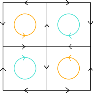
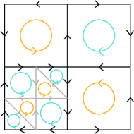
Figure 3. The mixing flow in four adjacent squares, as the cellular flow (left) is switched to the time-wasting flow (right) in one of them at $t_{nij}\in[n,n+\frac{1}{2}]$.

For $t\in(t_{nij},n+\tfrac{1}{2}]$, we let $u$ in $Q_{nij}$ be the “time-wasting” flow (see Figure 3)

$$u(x,y,t)=\nabla^{\perp}\left[(-1)^{i+j}\,2^{-2n}\eta\big{(}2^{n}x-i,2^{n}y-j\big{)}\right].$$ (2.8)

Proposition 2.3(1) shows that this flow does not cross $\partial Q_{nij}^{\prime}$ and $\partial Q_{nij}^{\prime\prime}$, hence

$$\int_{Q_{nij}^{\prime}}\rho\left(x,y,n+\frac{1}{2}\right)dxdy=0=\int_{Q_{nij}^{\prime\prime}}\rho\left(x,y,n+\frac{1}{2}\right)dxdy.$$

The flow for $t\in(n+\tfrac{1}{2},n+1]$ is constructed in the same fashion, but with the role of $Q_{nij}$ played by both $Q_{nij}^{\prime}$ and $Q_{nij}^{\prime\prime}$. That is, we decompose $Q$ into $2^{2n+1}$ identical rectangles $\tilde{Q}_{nij}:=(2^{-(n+1)}i,2^{-(n+1)}(i+1))\times(2^{-n}j,2^{-n}(j+1))$, so that by the above $\int_{\tilde{Q}_{nij}}\rho\left(x,y,n+\frac{1}{2}\right)dxdy=0$ for each of them. In each $\tilde{Q}_{nij}$ we let

$$u(x,y,t)=\begin{cases}\nabla^{\perp}\left[(-1)^{i+j}2^{-(2n+1)}\psi\big{(}2^{n+1}x-i,2^{n}y-j\big{)}\right]&t\in(n+\tfrac{1}{2},\tilde{t}_{nij}],\\ \nabla^{\perp}\left[(-1)^{i+j}2^{-(2n+1)}\eta\big{(}2^{n+1}x-i,2^{n}y-j\big{)}\right]&t\in(\tilde{t}_{nij},n+1],\end{cases}$$

where $\tilde{t}_{nij}\in[n+\tfrac{1}{2},n+1]$ is such that $\int_{\tilde{Q}_{nij}^{\prime}}\rho(x,y,\tilde{t}_{nij})dxdy=0$, with $\tilde{Q}_{nij}^{\prime}$ the lower half of $\tilde{Q}_{nij}$. It follows that $\int_{Q_{(n+1)ij}}\rho(x,y,n+1)dxdy=0$ for any $i,j\in\{0,\ldots,2^{n+1}-1\}$ and the induction step is completed.

Finally, $u$ is obviously incompressible and satisfies the no-flow condition on $\partial Q$. Moreover, for $t\in(n,n+\tfrac{1}{2}]$, $u$ is continuous on all of $Q$ except of the corners and centers of the squares $Q_{nij}$ and the centers of their sides. This is because Propositions 2.1(1) and 2.3(1), and the factor $(-1)^{i+j}$, show that each couple of neighboring squares have the same velocity (of magnitude $4\cdot 2^{-n}$) on their common boundary (except at its center). Since $\|\nabla u(\cdot,t)\|_{L^{p}(Q_{nij})}^{p}$ is clearly either $2^{-2n}\|\nabla^{2}\psi\|_{L^{p}(Q)}^{p}$ or $2^{-2n}\|\nabla^{2}\eta\|_{L^{p}(Q)}^{p}$ for each $Q_{nij}$ and each $t\in(n,n+\tfrac{1}{2}]$, it follows that $\|\nabla u(\cdot,t)\|_{p}$ is between $\|\nabla^{2}\psi\|_{p}$ and $\|\nabla^{2}\eta\|_{p}$ for these $t$. A similar argument applies to $t\in(n+\tfrac{1}{2},n+1]$, with the speeds being $2^{1-n}$ and $2^{2-n}$ on the horizontal and vertical boundaries of the $\tilde{Q}_{nij}$, respectively. Thus $\sup_{t>0}\|\nabla u(\cdot,t)\|_{p}\leq C_{p}^{\prime}:=2\max\{\|\nabla^{2}\psi\|_{p},\|\nabla^{2}\eta\|_{p}\}$, and Propositions 2.1(2) and 2.3(2) yield $C_{p}^{\prime}<\infty$ for $p<2$. ∎

3. Perfect mixing for no-flow boundary conditions and $p<\frac{3+\sqrt{5}}{2}$

For $p\geq 2$ we can no longer directly use the stream functions $\psi,\eta$ from the last section since $\nabla^{2}\psi,\nabla^{2}\eta\notin L^{2}(Q)$. This is because $|\nabla^{2}\varphi(x,y)|$ (with $\varphi$ from Lemma 2.2) is inversely proportional to the distance of $(x,y)$ to the nearest corner of $Q$, and $|\nabla^{2}\eta|$ diverges in the same manner near each of the 9 points in Figure 2. We will therefore modify $\varphi,\eta$ near their respective problematic points to circumvent this issue, and then adjust $\psi$ accordingly. Notice that this means that we also need to modify $\varphi$ near the four centers of the sides of $Q$, to match a cellular and a time-wasting flow in two neighboring cells.

Lemma 3.1.

Let $P$ be the set containing the four corners of $Q$ and the four centers of its sides, and let $d_{P}(x,y):=dist((x,y),P)$ for $(x,y)\in\bar{Q}$. Let $f\in C^{\infty}({\mathbb{R}}^{+}_{0})$ be a non-decreasing function with $f(s)=5s$ for $s\in[0,\tfrac{1}{10}]$ and $f(s)=1$ for $s\geq\tfrac{1}{5}$. Let

$$\varphi_{a}(x,y)=\varphi(x,y)f(d_{P}(x,y))^{a},$$ (3.1)

where $\varphi$ is from (2.1). If $a\in(0,1]$, then $\varphi_{a}$ satisfies:

1. $\varphi_{a}>0$ on Q, $\varphi_{a}=0$ on $\partial Q$, $\nabla\varphi_{a}\in L^{\infty}(Q)$, and $\partial_{n}\varphi_{a}=-4f(d_{P}(x,y))^{a}$ on $\partial Q_{c}$;

2. $\nabla^{2}\varphi_{a}\in L^{p}(Q)$ for $a\in(0,1)$ and all $p\in[1,\tfrac{2}{1-a})$, and $\nabla^{2}\varphi_{1}\in L^{\infty}(Q)$;

3. the level set $\{\varphi_{a}=s\}$ for each $s\in[0,\tfrac{2}{\pi})$ is a simple closed curve and for $s=\tfrac{2}{\pi}$ it is the point $(\tfrac{1}{2},\tfrac{1}{2})$, and for $a\in(0,1)$ we have $\sup_{s\in[0,2/\pi]}T_{\varphi_{a}}(s)<\infty$;

4. $T_{\varphi_{a}}$ is differentiable on $(0,\tfrac{2}{\pi})$ and $\sup_{s\in(0,2/\pi)}s^{2a/(a+1)}|T_{\varphi_{a}}^{\prime}(s)|\sup_{\{\varphi_{a}=s\}}|\nabla\varphi_{a}|^{2}<\infty$.

Figure 4 shows a comparison of the level sets of $\varphi$ and $\varphi_{a}$.

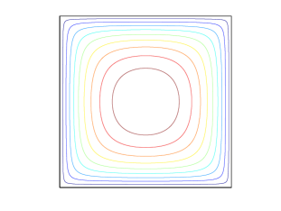
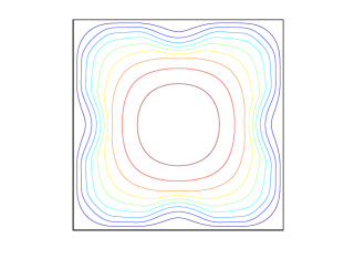
Figure 4. Level sets of $\varphi$ (left) and of $\varphi_{a}$ with $a=0.9$ (right).

Just as with Lemma 2.2, we postpone the proof of Lemma 3.1 to the appendix. Once we have $\varphi_{a}$, we can proceed as in Proposition 2.1 and define a corresponding stream function $\psi_{a}$ whose period $T_{\psi_{a}}(s)=1$ for each level set $\{\psi_{a}=s\}$.

Proposition 3.2.

For any $a\in(0,1)$ and $\varphi_{a}$ from (3.1), let

$$\psi_{a}(x,y):=\int_{0}^{\varphi_{a}(x,y)}T_{\varphi_{a}}(s)ds.$$ (3.2)

Then $\psi_{a}\in C(\bar{Q})$, $\nabla\psi_{a}$ is continuous on $\bar{Q}_{c}$ and differentiable on $Q\setminus\{(\tfrac{1}{2},\tfrac{1}{2})\}$, and:

1. $\psi_{a}>0$ on Q, $\psi_{a}=0$ on $\partial Q$, $\nabla\psi_{a}\in L^{\infty}(Q)$, and $\partial_{n}\psi_{a}(x,y)=-4T_{\varphi_{a}}(0)f(d_{P}(x,y))^{a}$ for $(x,y)\in\partial Q_{c}$;

2. $\nabla^{2}\psi_{a}\in L^{p}(Q)$ for all $p\in[1,\min\{\frac{2}{1-a},\frac{a+1}{2a}\})$;

3. the level set $\{\psi_{a}=s\}$ for each $s\in[0,\|\psi\|_{\infty})$ is a simple closed curve and for $s=\|\psi_{a}\|_{\infty}$ it is the point $(\tfrac{1}{2},\tfrac{1}{2})$, and $T_{\psi_{a}}(s)=1$ for each $s\in[0,\|\psi_{a}\|_{\infty}]$.

Proof.

The properties of $\nabla\psi_{a}$ and (1) are immediate from Lemma 3.1(1,3) and

$$\nabla\psi_{a}(x,y)=\nabla\varphi_{a}(x,y)\,T_{\varphi_{a}}(\varphi_{a}(x,y)).$$ (3.3)

The proof of (3) is identical to that of Proposition 2.1(3). Finally, differentiating (3.3) yields

$$|\nabla^{2}\psi_{a}|\leq\underbrace{|\nabla^{2}\varphi_{a}|\,T_{\varphi_{a}}(\varphi_{a}(x,y))}_{=:A(x,y)}+\underbrace{|\nabla\varphi_{a}|^{2}|T^{\prime}_{\varphi_{a}}(\varphi_{a}(x,y))|}_{=:B(x,y)}.$$ (3.4)

By Lemma 3.1(2,3) we have $A\in L^{p}(Q)$ for $p<\frac{2}{1-a}$. Lemma 3.1(1,3,4) and the co-area formula show for any $p<\tfrac{a+1}{2a}$ and some $C<\infty$ (depending on $p,a$),

$$\frac{1}{C}\int_{Q}B^{p}dxdy\leq\int_{Q}\varphi_{a}^{-\frac{2ap}{a+1}}dxdy=\int_{0}^{2/\pi}s^{-\frac{2ap}{a+1}}\int_{\{\varphi_{a}=s\}}\frac{1}{|\nabla\varphi_{a}|}d\sigma ds=\int_{0}^{2/\pi}s^{-\frac{2ap}{a+1}}T_{\varphi_{a}}(s)ds<\infty.$$

Hence $B\in L^{p}(Q)$ for these $p$ and (2) also follows. ∎

We next define a time-wasting flow $\eta_{a}$ with $\nabla\eta_{a}=\nabla\psi_{a}$ on $\partial Q_{cc}$.

Proposition 3.3.

For any $a\in(0,1)$, there exists a stream function $\eta_{a}\in C(\bar{Q})$, with $\nabla\eta_{a}$ continuous on $\bar{Q}_{cc}$ and differentiable on $Q\setminus\left(\{x=\tfrac{1}{2}\}\cup\{y=\tfrac{1}{2}\}\cup\{x+y=\tfrac{1}{2}\}\cup\{x+y=\tfrac{3}{2}\}\right)$, such that:

1. $\eta_{a}=0$ on $\partial Q\cup\{x=\tfrac{1}{2}\}\cup\{y=\tfrac{1}{2}\}$, $\nabla\eta_{a}\in L^{\infty}(Q)$, and $\partial_{n}\eta_{a}(x,y)=-4T_{\varphi_{a}}(0)f(d_{P}(x,y))^{a}$ for $(x,y)\in\partial Q_{cc}$;

2. $\nabla^{2}\eta_{a}\in L^{p}(Q)$ for all $p\in[1,\tfrac{2}{1-a})$.

Proof.

Let $\eta$ be from Proposition 2.3, $\tilde{P}:=P\cup\{(\frac{1}{2},\frac{1}{2})\}$ (with $P$ from Lemma 3.1), and

$$\eta_{a}(x,y):=T_{\varphi_{a}}(0)\eta(x,y)f(d_{\tilde{P}}(x,y))^{a}$$

for $(x,y)\in Q$. Then all the claims follow from the same properties for $\eta$ (with (2) proved as Lemma 3.1(2)). ∎

We can now repeat the proof of Theorem 2.4, this time using the stream functions $\psi_{a},\eta_{a}$ instead of $\psi,\eta$. Proposition 3.2(2) suggests to pick $a\in(0,1)$ which maximizes $\min\{\frac{2}{1-a},\frac{a+1}{2a}\}$, that is, $a:=\sqrt{5}-2$. Then $\frac{2}{1-a}=\frac{a+1}{2a}=\tfrac{3+\sqrt{5}}{2}$, and we obtain the following improvement of Theorem 2.4, with $\nabla u(\cdot,t)\in L^{p}(Q)$ for all $p<\tfrac{3+\sqrt{5}}{2}$.

Theorem 3.4.

Theorem 2.4 holds with $p\in[1,2)$ replaced by $p\in[1,\tfrac{3+\sqrt{5}}{2})$.

Remark. In fact, since we take $a=\sqrt{5}-2$ for all $p\in[1,\tfrac{3+\sqrt{5}}{2})$, the proof shows that our flow $u$ is independent of $p\in[1,\tfrac{3+\sqrt{5}}{2})$, in addition to being independent of $\kappa,\varepsilon\in(0,\tfrac{1}{2}]$.

4. Mixing for no-flow boundary conditions and $p\geq\frac{3+\sqrt{5}}{2}$

For $p\geq\frac{3+\sqrt{5}}{2}$, the construction from the previous section does not work because of the behavior of $\nabla^{2}\psi_{a}$ at $\partial Q$. Indeed, the term $|\nabla^{2}\varphi_{a}|$ on the right hand side of (3.4) blows up as $d_{P}(x,y)^{a-1}$ (with $d_{P}$ from Lemma 3.1) near the set $P$ by (A.10), while $|T^{\prime}_{\varphi_{a}}(s)|\sim s^{-2a/(a+1)}$ at $s=0$ (i.e., near $\partial Q$) by Lemma 3.1(4). For both these to be in $L^{p}$, one needs $(1-a)p<2$ and $\tfrac{2a}{a+1}p<1$, but such $a$ exists only for $p<\frac{3+\sqrt{5}}{2}$.

A solution to this problem is to “give up” on a small neighborhood of $\partial Q$, and not require the period of our stream functions to be 1 on the streamlines with $s\lesssim\delta$, for some $\delta>0$. (The affected region will have area $\sim\delta$. We can then choose $\delta\sim\kappa|\log(\kappa\varepsilon)|^{-1}$, so a flow analogous to that from the proof of Theorem 2.4 will still $\kappa$-mix $\rho_{0}$ to scale $\varepsilon$ in time $\sim|\log(\kappa\varepsilon)|$, although the bound on $\|\nabla u(\cdot,t)\|_{p}$ will now also depend on $\delta$.)

Remark. The easiest way of doing this is by replacing in the proof of Theorem 2.4 the stream functions $\psi$ and $\eta$ by $\psi^{\delta}(x,y):=\psi(x,y)f(\psi(x,y)/\delta)$ and 0, with $\delta>0$ small and $f$ from Lemma 3.1. Then $\nabla^{\perp}\psi^{\delta}=0$ on $\partial Q$ (which is why we can do not need a time-wasting flow), and properties of $\varphi,\psi$ show that $\sup_{\delta>0}\delta^{1-1/p}\|\nabla^{2}\psi^{\delta}\|_{p}<\infty$ for all $p\in[1,\infty]$ (see the proof of Lemma 6.1). Notice that now we have $T_{\psi^{\delta}}(s)=1$ for $s\geq\delta$ because $\psi^{\delta}=\psi$ on $D_{\delta}:=\{\psi>\delta\}$ (with $|Q\setminus D_{\delta}|\leq C\delta$). The times $t_{nij}\in[n,n+\tfrac{1}{2}]$ (and similarly $\tilde{t}_{nij}$) are now chosen so that $\int_{Q_{nij}^{\prime}\cap D_{nij}}\rho(x,y,t_{nij})dxdy=\int_{Q_{nij}^{\prime\prime}\cap D_{nij}}\rho(x,y,t_{nij})dxdy$, with $D_{nij}\subseteq Q_{nij}$ being the image of $D_{\delta}$ under the translation+dilation taking $Q$ to $Q_{nij}$ (so $|D_{nij}|\geq(1-C\delta)2^{-2n}$). This yields $|\int_{Q_{nij}^{\prime}}\rho(x,y,n+\tfrac{1}{2})dxdy-\tfrac{1}{2}\int_{Q_{nij}}\rho(x,y,n)dxdy|\leq\tfrac{C\delta}{2}2^{-2n}\|\rho_{0}\|_{\infty}$, and eventually $|\fint_{Q_{nij}}\rho(x,y,n)dxdy|\leq 4Cn\delta\|\rho_{0}\|_{\infty}$ via induction on $n$ (the details of this argument are spelled out in the proof of Theorem 4.3). Choosing again $n=\tau_{\kappa,\varepsilon}\sim|\log(\kappa\varepsilon)|$ and then $\delta\sim\tfrac{\kappa}{n}$ yields $\kappa$-mixing to scale $\varepsilon$ in time $\tau_{\kappa,\varepsilon}$ by a flow $u$ with $\sup_{t>0}\|\nabla u(\cdot,t)\|_{p}\leq C_{p}(\tfrac{|\log(\kappa\varepsilon)|}{\kappa})^{1-1/p}$. It follows that Theorem 2.4 holds (for all $p\in[1,\infty]$ and any of our three boundary conditions) with the right-hand side of (2.6) being $C_{p}\kappa^{-1+1/p}|\log(\kappa\varepsilon)|^{2-1/p}$. We will now show how to improve this estimate for no-flow boundary conditions, and also make the power of $|\log(\kappa\varepsilon)|$ converge to 1 as $p\downarrow\tfrac{3+\sqrt{5}}{2}$, in two steps. In Section 5 we treat the other boundary conditions.

For the sake of simplicity, let us start with the case $p=\infty$.

Proposition 4.1.

For any $a\in(0,1)$, $\delta\in(0,\tfrac{1}{10})$, there is a stream function $\psi_{a,\delta}\in C(\bar{Q})$, with $\nabla\psi_{a,\delta}$ continuous on $\bar{Q}_{c}$ and differentiable on $Q\setminus\{(\tfrac{1}{2},\tfrac{1}{2})\}$, such that:

1. $\psi_{a,\delta}>0$ on Q, $\psi_{a,\delta}=0$ on $\partial Q$, $\nabla\psi_{a,\delta}\in L^{\infty}(Q)$, and $\partial_{n}\psi_{a,\delta}(x,y)=-N_{a,\delta}(d_{P}(x,y))$ for $(x,y)\in\partial Q_{c}$, for some function $N_{a,\delta}:[0,\tfrac{1}{4}]\to[0,\infty)$;

2. $\sup_{\delta\in(0,1/10)}\delta^{\max\{1-a,2a\}/(a+1)}\|\nabla^{2}\psi_{a,\delta}\|_{\infty}<\infty$ for each $a\in(0,1)$;

3. there exists $s_{a,\delta}>0$, with $|\{\psi_{a,\delta}<s_{a,\delta}\}|\leq\delta$ such that the level set $\{\psi_{a,\delta}=s\}$ for each $s\in[s_{a,\delta},\|\psi_{a,\delta}\|_{\infty})$ is a simple closed curve and for $s=\|\psi_{a,\delta}\|_{\infty}$ it is the point $(\tfrac{1}{2},\tfrac{1}{2})$, and $T_{\psi_{a,\delta}}(s)=1$ for each $s\in[s_{a,\delta},\|\psi_{a,\delta}\|_{\infty}]$.

Proof.

For any $a\in(0,1)$ and $\delta\in(0,\frac{1}{10})$, let $D_{a,\delta}:=\{(x,y)\in Q:\varphi_{a}(x,y)>\delta\}$, with $\varphi_{a}$ from Lemma 3.1. All constants below may depend on $a$ but not on $\delta$, unless specified.

The co-area formula and Lemma 3.1(3) give for some $C<\infty$,

$$|Q\setminus D_{a,\delta}|=\int_{0}^{\delta}\int_{\{\varphi_{a}=s\}}\frac{1}{|\nabla\varphi_{a}|}d\sigma ds=\int_{0}^{\delta}T_{\varphi_{a}}(s)ds\leq C\delta,$$ (4.1)

and by (A.9) we also have for some $c>0$ that $d_{a,\delta}:=c\delta^{1/(a+1)}$ satisfies

$$d_{a,\delta}\leq\inf_{(x,y)\in D_{a,\delta/2}}d_{P}(x,y)\quad(<1).$$ (4.2)

With $f$ from Lemma 3.1, we now let

$$\varphi_{a,\delta}(x,y):=\varphi_{a}(x,y)\,f\left(\frac{d_{P}(x,y)}{d_{a,\delta}}\right)^{1-a},$$ (4.3)

so that $\varphi_{a,\delta}=\varphi_{a}$ when $d_{P}(x,y)\geq\tfrac{1}{5}d_{a,\delta}$ (and in particular, on $D_{a,\delta/2}$). Since

$$\varphi_{a,\delta}(x,y)=5d_{a,\delta}^{a-1}\varphi(x,y)d_{P}(x,y)=5d_{a,\delta}^{a-1}\varphi_{1}(x,y)$$

when $d_{P}(x,y)\leq\tfrac{1}{10}d_{a,\delta}$, from (A.10) for $a=1$ we obtain $|\nabla^{2}\varphi_{a,\delta}(x,y)|\leq Cd_{a,\delta}^{a-1}$ (for some $C<\infty$) when $d_{P}(x,y)\leq\frac{1}{10}d_{a,\delta}$. The same bound holds when $d_{P}(x,y)\in(\frac{1}{10}d_{a,\delta},\frac{1}{5}d_{a,\delta})$, due to (3.1), (A.9), and (A.10). By this and (A.10) for $a$, it follows for some $C<\infty$ (that changes between inequalities) and all $(x,y)\in Q$,

$$|\nabla^{2}\varphi_{a,\delta}(x,y)|\leq C\min\{d_{P}(x,y)^{a-1},d_{a,\delta}^{a-1}\}\leq C\min\{d_{P}(x,y)^{a-1},\delta^{(a-1)/(a+1)}\}.$$ (4.4)

Note also that $\partial_{n}\varphi_{a,\delta}(x,y)=-4f(d_{P}(x,y))^{a}f(d_{P}(x,y)/d_{a,\delta})^{1-a}$ on $\partial Q_{c}$. For later use we also mention that (4.3), Lemma 3.1(1), and $\varphi(x,y)d_{a,\delta}^{-1}\leq\tfrac{1}{5}\|\nabla\varphi\|_{\infty}$ for $d_{P}(x,y)<\tfrac{1}{5}d_{a,\delta}$ yield

$$\sup_{\delta\in(0,1/10)}\|\nabla\varphi_{a,\delta}\|_{\infty}<\infty.$$ (4.5)

We now construct a new stream function $\psi_{a,\delta}$ by making the periods of all streamlines of $\varphi_{a,\delta}$ contained in $D_{a,\delta}$ (where $\varphi_{a,\delta}=\varphi_{a}$) to be 1. We let

$$T_{a,\delta}(s):=\begin{cases}T_{\varphi_{a}}(\delta)&s\in[0,\tfrac{\delta}{2}],\\ T_{\varphi_{a}}(s)&s\in[\delta,\tfrac{2}{\pi}],\end{cases}$$

and choose $T_{a,\delta}$ on $(\tfrac{\delta}{2},\delta)$ so that $T_{a,\delta}$ is differentiable on $(0,\tfrac{2}{\pi})$,

$$\sup_{s\leq\delta}|T_{a,\delta}(s)-T_{a,\delta}(\delta)|\leq\frac{T_{a,\delta}(\delta)}{2}\qquad\text{and}\qquad\sup_{s\leq\delta}|T_{a,\delta}^{\prime}(s)|\leq|T_{\varphi_{a}}^{\prime}(\delta)|.$$ (4.6)

(We could have instead chosen $T_{a,\delta}(s)=T_{\varphi_{a}}(\delta)$ for $s\in[0,\delta)$, at the expense of $\nabla\psi_{a,\delta}$ not being differentiable on the streamline $\{\varphi_{a}=\delta\}$. This would not change our main results.) We now define

$$\psi_{a,\delta}(x,y):=\int_{0}^{\varphi_{a,\delta}(x,y)}T_{a,\delta}(s)ds.$$

The properties of $\nabla\psi_{a,\delta}$ and (1) immediately follow from the properties of $\varphi_{a}$ and $f$, with $N_{a,\delta}(r):=4f(r)^{a}f(\tfrac{r}{d_{a,\delta}})^{1-a}T_{\varphi_{a}}(\delta)$. Part (3) holds with $s_{a,\delta}:=\int_{0}^{\delta}T_{a,\delta}(s)ds$ and the estimate $|\{\psi_{a,\delta}<s_{a,\delta}\}|\leq C\delta$ (which is sufficient because then one only needs to replace $\psi_{a,\delta}$ by $\psi_{a,\delta/C}$), due to (4.1) and because $\psi_{a,\delta}-\psi_{a}$ is constant on $D_{a,\delta}=\{\psi_{a,\delta}>s_{a,\delta}\}$ (since $\varphi_{a,\delta}=\varphi_{a}$ there).

To show (2), notice that on $D_{a,\delta/2}$ we have by (A.10), Lemma 3.1(3,4), (4.6), and (4.2),

$$\begin{split}|\nabla^{2}\psi_{a,\delta}|&\leq|\nabla^{2}\varphi_{a}|\,T_{a,\delta}(\varphi_{a}(x,y))+|\nabla\varphi_{a}|^{2}|T_{a,\delta}^{\prime}(\varphi_{a}(x,y))|\\ &\leq Cd_{P}(x,y)^{a-1}+C\varphi_{a}(x,y)^{-2a/(a+1)}\\ &\leq C\delta^{-\max\{1-a,2a\}/(a+1)},\end{split}$$

where $C<\infty$ changes between inequalities. On $Q\setminus D_{a,\delta/2}$ we have $\psi_{a,\delta}=T_{a,\delta}(\delta)\varphi_{a,\delta}$, so (4.4) and Lemma 3.1(3) yield $|\nabla^{2}\psi_{a,\delta}|\leq C\delta^{(a-1)/(a+1)}$ there. These two estimates prove (2). ∎

We also define the time-wasting flow corresponding to $\psi_{a,\delta}$.

Proposition 4.2.

For any $a\in(0,1)$, $\delta\in(0,\tfrac{1}{10})$, there is a stream function $\eta_{a,\delta}\in C(\bar{Q})$, with $\nabla\eta_{a,\delta}$ continuous on $\bar{Q}_{cc}$ and differentiable on $Q\setminus\left(\{x=\tfrac{1}{2}\}\cup\{y=\tfrac{1}{2}\}\cup\{x+y=\tfrac{1}{2}\}\cup\{x+y=\tfrac{3}{2}\}\right)$, such that:

1. $\eta_{a,\delta}=0$ on $\partial Q\cup\{x=\tfrac{1}{2}\}\cup\{y=\tfrac{1}{2}\}$, $\nabla\eta_{a,\delta}\in L^{\infty}(Q)$, and $\partial_{n}\eta_{a,\delta}(x,y)=-N_{a,\delta}(d_{P}(x,y))$ for $(x,y)\in\partial Q_{cc}$, with the function $N_{a,\delta}$ from Proposition 4.1;

2. $\sup_{\delta\in(0,1/10)}\delta^{\max\{1-a,2a\}/(a+1)}\|\nabla^{2}\eta_{a,\delta}\|_{\infty}<\infty$.

Proof.

Let

$$\eta_{a,\delta}(x,y):=\eta_{a}(x,y)f\left(\frac{d_{P}(x,y)}{d_{a,\delta}}\right)^{1-a}T_{\varphi_{a}}\left(\delta\right),$$

where $d_{a,\delta}$ is from the previous proof. Then (1) follows from Proposition 3.3(1) and the definition of $N_{a,\delta}$, and (2) is proved as Proposition 4.1(2). ∎

Next, let us first obtain a weaker result for $p=\infty$, with a $\sim|\log(\kappa\varepsilon)|^{3/2}$ bound. Afterwards, we will include an additional element to improve the bound to $\sim|\log(\kappa\varepsilon)|^{4/3}=|\log(\kappa\varepsilon)|^{1+\nu_{\infty}}$.

Theorem 4.3.

For any mean-zero $\rho_{0}\in L^{\infty}(Q)$ and any $\kappa,\varepsilon\in(0,\tfrac{1}{2}]$, there is an incompressible flow $u:Q\times{\mathbb{R}}^{+}\to\mathbb{R}^{2}$ with $u\cdot n=0$ on $\partial Q\times{\mathbb{R}}^{+}$ which $\kappa$-mixes $\rho_{0}$ to scale $\varepsilon$ in a time $\tau_{\kappa,\varepsilon}$ satisfying

$$\int_{0}^{\tau_{\kappa,\varepsilon}}\|\nabla u(\cdot,t)\|_{\infty}\,dt\leq C\kappa^{-1/2}|\log(\kappa\varepsilon)|^{3/2},$$ (4.7)

with a universal $C<\infty$. The flow can be made independent of $\varepsilon$ if the right-hand side of (4.7) is replaced by $C\kappa^{-1/2}|\log(\kappa\varepsilon)|^{3/2}\log|\log(\kappa\varepsilon)|$.

Proof.

Let $a:=\tfrac{1}{3}$ (which minimizes the power in Proposition 4.1(2), to $\tfrac{1}{2}$), fix some $\delta\in(0,\tfrac{1}{10})$ (to be chosen later), and let $\psi_{a,\delta},\eta_{a,\delta}$ be the corresponding stream functions from Propositions 4.1 and 4.2. The construction of $u$ is now almost identical to the proof of Theorem 2.4, with $\psi,\eta$ replaced by $\psi_{a,\delta},\eta_{a,\delta}$. The one change is that Proposition 4.1(3) only guarantees for each $n$ and any square $Q_{nij}$ (with $Q_{nij}^{\prime},Q_{nij}^{\prime\prime}$ its left and right halves) existence of $t_{nij}\in[n,n+\tfrac{1}{2}]$ such that $\int_{Q_{nij}^{\prime}\cap D_{nij}}\rho(x,y,t_{nij})dxdy=\int_{Q_{nij}^{\prime\prime}\cap D_{nij}}\rho(x,y,t_{nij})dxdy$, with the set $D_{nij}\subseteq Q_{nij}$ such that $|D_{nij}|\geq(1-\delta)2^{-2n}$ (in fact, $D_{nij}$ is the image of the set $D_{a,\delta}=\{\psi_{a,\delta}>s_{a,\delta}\}$ under the translation+dilation taking $Q$ to $Q_{nij}$). We thus find that $|\int_{Q_{nij}^{\prime}}\rho(x,y,n+\tfrac{1}{2})dxdy-\tfrac{1}{2}\int_{Q_{nij}}\rho(x,y,n)dxdy|\leq\tfrac{\delta}{2}2^{-2n}\|\rho_{0}\|_{\infty}$.

A similar adjustment is made when finding the time $\tilde{t}_{nij}$ as in the proof of Theorem 2.4. We thus find that for any of the four squares with side length $2^{-(n+1)}$ which form $Q_{nij}$ (call it $\tilde{Q}$) we have

$$\left|\fint_{\tilde{Q}}\rho(x,y,n+1)dxdy-\fint_{Q_{nij}}\rho(x,y,n)dxdy\right|\leq 4\delta\|\rho_{0}\|_{\infty}.$$ (4.8)

Since $\rho_{0}$ is mean-zero, it follows by induction on $n$ that

$$\left|\fint_{Q_{nij}}\rho(x,y,n)dxdy\right|\leq 4n\delta\|\rho_{0}\|_{\infty}.$$

We now construct this flow on the time interval $[0,n]$, with $n:=\tau_{\kappa,\varepsilon}:=\lceil|\log_{2}\tfrac{\kappa\varepsilon}{2}|\rceil+2$ (then it is easily shown that for any $(x,y)\in Q$, the squares $Q_{nij}$ which are fully contained in $B_{\varepsilon}(x,y)\cap Q$ have total area $\geq(1-\tfrac{\kappa}{2})|B_{\varepsilon}(x)\cap Q|$) and with $\delta:=\frac{\kappa}{8n}$, which then obviously $\kappa$-mixes $\rho_{0}$ to scale $\varepsilon$ in time $\tau_{\kappa,\varepsilon}$. As in the proof of Theorem 2.4, but using Propositions 4.1(2) and 4.2(2), it follows that $\sup_{t\in(0,n]}\|\nabla u(\cdot,t)\|_{\infty}\leq C^{\prime}\delta^{-1/2}$ for some universal $C^{\prime}<\infty$. This yields the first claim because $C^{\prime}\delta^{-1/2}\tau_{\kappa,\varepsilon}\leq C\kappa^{-1/2}|\log(\kappa\varepsilon)|^{3/2}$ for some universal $C$.

If we instead want the flow to be independent of $\varepsilon$, we use on each time interval $[n,n+1]$ the flows $\psi_{1/3,\delta_{n}},\eta_{1/3,\delta_{n}}$, with some $\delta_{n}>0$ to be chosen. We then obtain

$$\left|\fint_{Q_{nij}}\rho(x,y,n)dxdy\right|\leq 4\|\rho_{0}\|_{\infty}\sum_{k=0}^{n-1}\delta_{k},$$ (4.9)

and $\sup_{t\in(n,n+1]}\|\nabla u(\cdot,t)\|_{\infty}\leq C^{\prime}\delta_{n}^{-1/2}$. We again choose $n:=\tau_{\kappa,\varepsilon}:=\lceil|\log_{2}\tfrac{\kappa\varepsilon}{2}|\rceil+2$, and then $\delta_{k}$ such that $\sum_{k=0}^{\infty}\delta_{k}\leq\tfrac{\kappa}{8}$, so that the obtained flow again $\kappa$-mixes $\rho_{0}$ to any scale $\varepsilon\in(0,\tfrac{1}{2}]$ in time $\tau_{\kappa,\varepsilon}$. We now make the specific choice $\delta_{k-2}:=\tfrac{\kappa}{M}k^{-1}(\log k)^{-2}$ for $k\geq 2$, with $M:=8\sum_{k=2}^{\infty}k^{-1}(\log k)^{-2}$. Then the integral in (4.7) is bounded by $C^{\prime}\sum_{k=0}^{n-1}\delta_{k}^{-1/2}$, which is no more than $C\kappa^{-1/2}|\log(\kappa\varepsilon)|^{3/2}\log|\log(\kappa\varepsilon)|$, for some large enough universal $C$. ∎

To achieve better mixing for $p=\infty$, we will next squeeze some mileage out of the sets $Q_{nij}\setminus D_{nij}$ from the previous proof, instead of simply “giving up” on them. To do this, we first need to obtain an estimate on the periods of the streamlines $\{\psi_{a,\delta}=s\}$ for $s\leq\delta$. This will say that even though these periods need not equal 1, most of them are still close to 1. The following property of $\varphi_{a,\delta}$, which we again prove in the appendix, will yield the estimate.

Lemma 4.4.

For any $a\in(0,1)$, $\delta\in(0,\tfrac{1}{10})$, the functions $\varphi_{a,\delta}$ from (4.3) satisfy:

1. the level set $\{\varphi_{a,\delta}=s\}$ for each $s\in[0,\tfrac{2}{\pi})$ is a simple closed curve;

2. $\sup_{0<s\leq\delta<1/10}(\delta^{(1-a)/(a+1)}\log\tfrac{2\delta}{s})^{-1}|T_{\varphi_{a,\delta}}(s)-T_{\varphi_{a}}(\delta)|<\infty$ for each $a\in(0,1)$.

We can now prove the final version of our result for $p=\infty$.

Theorem 4.5.

Theorem 4.3 holds with each $\kappa^{-1/2}|\log(\kappa\varepsilon)|^{3/2}$ replaced by $\kappa^{-1/3}|\log(\kappa\varepsilon)|^{4/3}$.

Proof.

We proceed identically to the proof of Theorem 4.3, but with a slightly different choice of the times $t_{nij}\in[n,n+\tfrac{1}{2}]$ (and also $\tilde{t}_{nij}\in[n+\tfrac{1}{2},n+1]$). Let us define

$$\tilde{\psi}_{a,\delta}(x,y):=\int_{0}^{\varphi_{a,\delta}(x,y)}T_{\varphi_{a,\delta}}(s)ds,$$

so that $T_{\tilde{\psi}_{a,\delta}}\equiv 1$ and $\tilde{\psi}_{a,\delta}-\psi_{a,\delta}$ is constant on $D_{a,\delta}=\{\varphi_{a,\delta}>\delta\}$. The latter means that if we let $u$ and $\tilde{u}$ be given on $Q_{nij}\times(n,t_{nij}]$ by (2.7) with $\psi_{a,\delta}$ and $\tilde{\psi}_{a,\delta}$ in place of $\psi$, respectively, then $u\equiv\tilde{u}$ on $D_{a,\delta}$. Notice that $u$ is the same as in Theorem 4.3.

Let us now pick, in the proof of Theorem 4.3, the time $t_{nij}$ so that if the flow in $Q_{nij}$ for $t\in(n,t_{nij}]$ were $\tilde{u}$, then we would have $\int_{Q_{nij}^{\prime}}\rho(x,y,t_{nij})dxdy=\int_{Q_{nij}^{\prime\prime}}\rho(x,y,t_{nij})dxdy$. This is possible because $\tilde{u}$ rotates $Q_{nij}$ by $180^{\circ}$ in time $\tfrac{1}{2}$. Having this new $t_{nij}$, we still use $u$ to transport $\rho$ for $t\in(n,t_{nij}]$ because $\nabla\tilde{u}=\nabla^{2}\tilde{\psi}_{a,\delta}\notin L^{\infty}(Q)$. This will introduce an error in the above equality of integrals of $\rho(\cdot,t_{nij})$ over $Q_{nij}^{\prime}$ and $Q_{nij}^{\prime\prime}$, which we estimate by using Lemma 4.4. After doing the same with $\tilde{t}_{nij}\in[n+\tfrac{1}{2},n+1]$, we eventually still obtain an estimate like (4.8), but with a better bound (see (4.14) below). This is because Lemma 4.4(2) shows that most streamlines of $\psi_{a,\delta}$ lying in $Q\setminus D_{a,\delta}$ still have their periods $T_{\psi_{a,\delta}}$ close to 1.

For the sake of simplicity, assume $n=0$ (so $Q_{nij}=Q$, $u=\nabla^{\perp}\psi_{a,\delta}$, $\tilde{u}=\nabla^{\perp}\tilde{\psi}_{a,\delta}$, and $t_{nij}=t_{000}\in[0,\tfrac{1}{2}]$), since the general case is identical. We have $u\equiv\tilde{u}$ on $D_{a,\delta}$ and, in fact,

$$\tilde{u}(x,y)=\frac{T_{\varphi_{a,\delta}}(\varphi_{a,\delta}(x,y))}{T_{a,\delta}(\varphi_{a,\delta}(x,y))}u(x,y)$$

on $Q$. This and the definition of $t_{000}$ above (which uses $\tilde{u}$ instead of $u$) mean that if $X(0;x,y)=(x,y)$ and $X_{t}(t;x,y)=U(X(t;x,y))$, with

$$U(x,y):=t_{000}(\tilde{u}(x,y)-u(x,y))=t_{000}\frac{T_{\varphi_{a,\delta}}(\varphi_{a,\delta}(x,y))-T_{a,\delta}(\varphi_{a,\delta}(x,y))}{T_{a,\delta}(\varphi_{a,\delta}(x,y))}u(x,y),$$ (4.10)

then $\rho$ solving (1.1) with $u$ (not $\tilde{u}$) satisfies

$$\int_{Q^{\prime}}\rho\left(X(1;x,y),t_{000}\right)dxdy=\int_{Q^{\prime\prime}}\rho\left(X(1;x,y),t_{000}\right)dxdy,$$

(where $Q^{\prime},Q^{\prime\prime}$ are the left and right halves of $Q$). We have $\nabla\cdot U\equiv 0$ because $U(x,y)=\nabla^{\perp}h(\varphi_{a,\delta}(x,y))$ for some function $h$, so $X(1;\cdot)$ is measure preserving and hence

$$\int_{X(1;Q^{\prime})}\rho\left(x,y,t_{000}\right)dxdy=\int_{X(1;Q^{\prime\prime})}\rho\left(x,y,t_{000}\right)dxdy.$$ (4.11)

We would like to replace $X(1;Q^{\prime}),X(1;Q^{\prime\prime})$ by $Q^{\prime},Q^{\prime\prime}$ here. To control the resulting error, we need to estimate the size of the symmetric difference of $X(1;Q^{\prime})$ and $Q^{\prime}$ (see (4.13) below).

The definition of $T_{a,\delta}$, Lemma 3.1(3), and (4.5) show that $\|u\|_{\infty}\leq C$ for some $\delta$-independent $C<\infty$. Since also $T_{a,\delta}(\varphi_{a,\delta}(x,y))^{-1}$ is bounded for $(x,y)$ near $\partial Q$, uniformly in $\delta\in(0,\tfrac{1}{10})$ (because $\nabla\varphi_{a}\in L^{\infty}(Q)$), we obtain from (4.10), the definition of $T_{a,\delta}$, and Lemma 4.4(2) that

$$|X(1;x,y)-(x,y)|\leq C\delta^{(1-a)/(a+1)}\log\frac{2\delta}{\varphi_{a,\delta}(x,y)}\qquad\text{when $0<\varphi_{a,\delta}(x,y)\leq\delta<\tfrac{1}{10}$,}$$ (4.12)

with $C$ independent of $\delta$ and $(x,y)$. (Of course, $X(1;x,y)=(x,y)$ when $\varphi_{a,\delta}(x,y)>\delta$.)

We claim that this shows that if $D_{l}:=\{2^{-l}\delta<\varphi_{a,\delta}<2^{1-l}\delta\}$ for $l\geq 1$ (each $D_{l}$ is obviously invariant under the flows $u,\tilde{u},U$), then

$$|\{(x,y)\in D_{l}\,:\,\text{exactly one of $(x,y)$ and $X(1;x,y)$ belongs to $Q^{\prime}$}\}|\leq c\delta^{2/(a+1)}\frac{l}{2^{l}}$$ (4.13)

for some $(\delta,l)$-independent $c<\infty$.

Assume this is true. Then $X(1;\cdot)$ being measure preserving and (4.11) show

$$\left|\int_{Q^{\prime}}\rho(x,y,t_{000})dxdy-\frac{1}{2}\int_{Q}\rho(x,y,0)dxdy\right|\leq\|\rho_{0}\|_{\infty}c\delta^{2/(a+1)}\sum_{l=1}^{\infty}\frac{l}{2^{l}}=:c^{\prime}\delta^{2/(a+1)}\|\rho_{0}\|_{\infty}.$$

Applying this for any $n\geq 0$ and any square $Q_{nij}$ (and then an analogous estimate involving $\tilde{t}_{nij}\in(n+\tfrac{1}{2},n+1]$), as in the proof of Theorem 4.3, we see that if $\tilde{Q}$ is any of the four squares with side length $2^{-(n+1)}$ which form $Q_{nij}$, then

$$\left|\fint_{\tilde{Q}}\rho(x,y,n+1)dxdy-\fint_{Q_{nij}}\rho(x,y,n)dxdy\right|\leq 8c^{\prime}\delta^{2/(a+1)}\|\rho_{0}\|_{\infty}.$$ (4.14)

As a result, (4.9) now becomes (for mean-zero $\rho_{0}$)

$$\left|\fint_{Q_{nij}}\rho(x,y,n)dxdy\right|\leq 8c^{\prime}\|\rho_{0}\|_{\infty}\sum_{k=0}^{n-1}\delta_{k}^{2/(a+1)}.$$ (4.15)

We can now proceed as in the proof of Theorem 4.3, again with $n:=\tau_{\kappa,\varepsilon}:=\lceil|\log_{2}\tfrac{\kappa\varepsilon}{2}|\rceil+2$. When the flow is allowed to depend on $\varepsilon$, we pick $\delta_{k}:=\delta:=(\frac{\kappa}{16c^{\prime}n})^{(a+1)/2}$, which then yields

$$\sup_{t\in(0,n]}\|\nabla u(\cdot,t)\|_{\infty}\leq C^{\prime}\delta^{-\max\{1-a,2a\}/(a+1)}\leq C^{\prime\prime}\left(\frac{|\log(\kappa\varepsilon)|}{\kappa}\right)^{\max\{1-a,2a\}/2}$$

for some $a$-dependent $C^{\prime},C^{\prime\prime}<\infty$. We minimize the power (to $\tfrac{1}{3}$) by again choosing $a:=\tfrac{1}{3}$, and the first claim of the theorem follows.

If we want the flow to be independent of $\varepsilon$, all is the same as in Theorem 4.3 but we need $\sum_{k=1}^{\infty}\delta_{k}^{2/(a+1)}\leq\tfrac{\kappa}{16c^{\prime}}$ instead of $\sum_{k=1}^{\infty}\delta_{k}\leq\tfrac{\kappa}{8}$. We pick again $a:=\tfrac{1}{3}$, so that $\delta_{k-2}:=(\tfrac{\kappa}{M}k^{-1}(\log k)^{-2})^{2/3}$ satisfies this when $M:=16c^{\prime}\sum_{k=2}^{\infty}k^{-1}(\log k)^{-2}$. Then the integral in (4.7) is bounded by $C^{\prime}\sum_{k=0}^{n-1}\delta_{k}^{-1/2}$, which is due to our choice of $n$ no more than $C\kappa^{-1/3}|\log(\kappa\varepsilon)|^{4/3}\log|\log(\kappa\varepsilon)|$, for some large enough universal $C$.

It remains to prove (4.13). The streamlines of $U$ are the level sets $\{\varphi_{a,\delta}=s\}$. Each of them is a simple closed curve, so each “moves” in a single direction. Also, $\{\varphi_{a,\delta}=s\}$ with $s<\tfrac{1}{10}$ intersects $\{x_{0}\}\times(0,\tfrac{1}{2})$ in exactly one point when $x_{0}\in[\tfrac{1}{4},\tfrac{3}{4}]$. For $0<s<s^{\prime}<\tfrac{1}{10}$, let

$$M_{s,s^{\prime}}({x_{0}}):=|\{\varphi_{a,\delta}(x,y)\in(s,s^{\prime})\,:\,X(t;x,y)\in\{x_{0}\}\times(0,\tfrac{1}{2})\text{ for some $t\in(0,1)$}\}|$$

be the measure of the set of those points between level sets $\{\varphi_{a,\delta}=s\}$ and $\{\varphi_{a,\delta}=s^{\prime}\}$ which cross the segment $\{x_{0}\}\times(0,\tfrac{1}{2})$ during time interval $(0,1)$ when advected by the flow $U$ (by the above, any point can cross at most once). Incompressibility of $U$ shows that $M_{s,s^{\prime}}$ must be constant on $[\tfrac{1}{4},\tfrac{3}{4}]$ for each $0<s<s^{\prime}<\tfrac{1}{10}$. We now pick $s:=2^{-l}\delta$ and $s^{\prime}:=2^{1-l}\delta$, and notice that the width of $D_{l}$ near $\{\tfrac{1}{4}\}\times(0,\tfrac{1}{2})$ is easily shown to be comparable to $2^{-l}\delta$. Hence

$$M_{2^{-l}\delta,2^{1-l}\delta}\left(\frac{1}{2}\right)=M_{2^{-l}\delta,2^{1-l}\delta}\left(\frac{1}{4}\right)\leq c\delta^{(1-a)/(a+1)}l\frac{\delta}{2^{l}}=c\delta^{2/(a+1)}\frac{l}{2^{l}}$$

by (4.12), with some $(\delta,l)$-independent $c<\infty$. Since the same bound is obtained if $M_{2^{-l}\delta,2^{1-l}\delta}$ is defined with $(\tfrac{1}{2},1)$ in place of $(0,\tfrac{1}{2})$, (4.13) follows if we replace $c$ by $2c$. ∎

The case $p\in[\frac{3+\sqrt{5}}{2},\infty)$ is almost identical to $p=\infty$, even simpler in a sense. We now let

$$\varphi_{a,\delta,p}(x,y)=\varphi_{a}(x,y)\,f\left(\frac{d_{P}(x,y)}{d_{a,\delta}}\right)^{1-a-\frac{2}{p}}\left(1-\log f\left(\frac{d_{P}(x,y)}{d_{a,\delta}}\right)\right)^{-1}$$

and define $\psi_{a,\delta,p}$ via $\varphi_{a,\delta,p}$ as in the proof of Proposition 4.1. That proposition then holds for $\psi_{a,\delta,p}$, with a different bound in (2). Indeed, essentially the same proof yields

$$\|\nabla^{2}\psi_{a,\delta,p}\|_{p}\leq C\delta^{-\max\left\{1-a-\tfrac{2}{p},2a-\tfrac{a+1}{p}\right\}/(a+1)}\quad\text{ for }p>\frac{3+\sqrt{5}}{2},$$

where the right-hand side is minimized (to $C\delta^{-(p^{2}-3p+1)/(2p^{2}-p)}$) when $a=\tfrac{p-1}{3p-1}$ (we fix this $a$ from now on). For $p=\frac{3+\sqrt{5}}{2}$ we get $\|\nabla^{2}\psi_{a,\delta,p}\|_{p}\leq C|\log\delta|^{1/p}$ when $a=\frac{p-1}{3p-1}=\sqrt{5}-2$.

Lemma 4.4 also holds for $p\in[\frac{3+\sqrt{5}}{2},\infty)$ and $a=\tfrac{p-1}{3p-1}$, with the estimate in part (2) being

$$\sup_{0<s\leq\delta<1/10}\delta^{-p/(2p-1)}|T_{\varphi_{a,\delta,p}}(s)-T_{\varphi_{a}}(\delta)|<\infty.$$

Notice that there is no $s$-dependence in the first term when $p<\infty$, which means that in the argument from the proof of Theorem 4.5 we do not need to split $\{\varphi_{a,\delta,p}\leq\delta\}$ into the sets $D_{l}$ anymore. That argument (which also uses the proof of Theorem 4.3) then yields

$$\left|\fint_{Q_{nij}}\rho(x,y,n)dxdy\right|\leq 8c^{\prime}\|\rho_{0}\|_{\infty}\sum_{k=0}^{n-1}\delta_{k}^{(3p-1)/(2p-1)}.$$

instead of (4.15) (notice that $1+\tfrac{p}{2p-1}=\tfrac{3p-1}{2p-1}$ replaces $1+\tfrac{1-a}{a+1}=\tfrac{2}{a+1}$). Then the end of the proof of Theorem 4.5 (before the proof of (4.13)) has $\delta_{k}^{2/(a+1)}$ and $\delta_{k}^{-1/2}$ replaced by $\delta_{k}^{(3p-1)/(2p-1)}$ and $\delta_{k}^{-(p^{2}-3p+1)/(2p^{2}-p)}$, respectively (the latter is $|\log\delta_{k}|^{1/p}$ when $p=\frac{3+\sqrt{5}}{2}$). We therefore pick $\delta_{k}:=(\tfrac{\kappa}{16c^{\prime}n})^{(2p-1)/(3p-1)}$ (or $\delta_{k-2}:=(\tfrac{\kappa}{M}k^{-1}(\log k)^{-2})^{(2p-1)/(3p-1)}$ in the $\varepsilon$-independent case, with $M:=16c^{\prime}\sum_{k=2}^{\infty}k^{-1}(\log k)^{-2}$) and obtain the following.

Theorem 4.6.

For any mean-zero $\rho_{0}\in L^{\infty}(Q)$ and any $\kappa,\varepsilon\in(0,\tfrac{1}{2}]$, there is an incompressible flow $u:Q\times{\mathbb{R}}^{+}\to\mathbb{R}^{2}$ with $u\cdot n=0$ on $\partial Q\times{\mathbb{R}}^{+}$ which $\kappa$-mixes $\rho_{0}$ to scale $\varepsilon$ in a time $\tau_{\kappa,\varepsilon}$ satisfying

$$\int_{0}^{\tau_{\kappa,\varepsilon}}\|\nabla u(\cdot,t)\|_{p}\,dt\leq\begin{cases}C_{p}\kappa^{-\nu_{p}}|\log(\kappa\varepsilon)|^{1+\nu_{p}}&p\in(\frac{3+\sqrt{5}}{2},\infty),\\ C_{p}|\log(\kappa\varepsilon)|\,\left|\log\frac{|\log(\kappa\varepsilon)|}{\kappa}\right|^{1/p}&p=\frac{3+\sqrt{5}}{2},\end{cases}$$ (4.16)

with $\nu_{p}:=\frac{p^{2}-3p-1}{3p^{2}-p}$ and $C_{p}<\infty$ depending only on $p$. The flow can be made independent of $\varepsilon$, but the $p\in(\frac{3+\sqrt{5}}{2},\infty)$ alternative of the right-hand side of (4.16) must be replaced by $C_{p}\kappa^{-\nu_{p}}|\log(\kappa\varepsilon)|^{1+\nu_{p}}\log|\log(\kappa\varepsilon)|$.

5. Mixing for periodic and no-slip boundary conditions

In this section we will show that the results from Sections 2–4 extend to periodic boundary conditions with only minor modifications to their proofs (in particular, “perfect” mixing is preserved here), and with some more work and slightly worse bounds also to no-slip boundary conditions. Let us start with the simpler case of periodic boundary conditions.

Theorem 5.1.

Theorems 3.4, 4.5, and 4.6 hold when the no-flow boundary condition $u\cdot n=0$ on $\partial Q\times{\mathbb{R}}^{+}$ is replaced by the periodic boundary condition.

Proof.

Notice that the flows from all three theorems already satisfy periodic boundary conditions at all times $t>1$. Hence the only change required will be for $t\in(0,1]$.

First consider the case from Theorem 3.4. What we need is that $\int_{Q_{1ij}}\rho(x,y,1)dxdy=0$ for any $i,j\in\{0,1\}$. We first let $u(x,y,t)=(2,0)$ for $t\in(0,t_{0}]$ and $u(x,y,t)=0$ for $t\in(t_{0},\tfrac{1}{4}]$, where $t_{0}\in[0,\tfrac{1}{4}]$ is such that $\int_{(0,1/2)\times(0,1)}\rho(x,y,t_{0})dxdy=0$ (which exists because the left and right halves of $Q$ would be swapped in time $\tfrac{1}{4}$. Now let

$$m_{0}:=\int_{Q_{100}}\rho(x,y,\tfrac{1}{4})dxdy=-\int_{Q_{101}}\rho(x,y,\tfrac{1}{4})dxdy,$$

$$m_{1}:=\int_{Q_{111}}\rho(x,y,\tfrac{1}{4})dxdy=-\int_{Q_{110}}\rho(x,y,\tfrac{1}{4})dxdy.$$

For $t\in[\frac{1}{4},\frac{3}{4})$ and $a:=\sqrt{5}-2$ (the latter as in Theorem 3.4), define

$$u(x,y,t)=\begin{cases}\nabla^{\perp}\left[(-1)^{i+j}2^{-2}\psi_{a}\big{(}2x-i,2y-j)\big{)}\right]&t\in(\tfrac{1}{4},t_{ij}],\\ \nabla^{\perp}\left[(-1)^{i+j}2^{-2}\eta_{a}\big{(}2x-i,2y-j)\big{)}\right]&t\in(t_{ij},\tfrac{3}{4}],\end{cases}$$

where $t_{ij}\in[\frac{1}{4},\frac{3}{4}]$ is such that the integrals of $\rho(\cdot,t_{ij})$ over the lower and upper halves of $Q_{1ij}$ are equal (then they are both $\tfrac{1}{2}(-1)^{i+j}m_{i}$). Finally, for $t\in(\frac{3}{4},1]$ we let $u(x,y,t)=(0,1)$, so that indeed $\int_{Q_{1ij}}\rho(x,y,1)dxdy=0$ for any $i,j\in\{0,1\}$, and we are done.

The case from Theorem 4.5 is virtually identical, with $\psi_{a},\eta_{a}$ replaced by $\psi_{a,\delta},\eta_{a,\delta}$ as in that theorem (i.e., $a=\tfrac{1}{3}$ and either $\delta=(\frac{\kappa}{16c^{\prime}n})^{(a+1)/2}$ when $u$ can depend on $\varepsilon$ or $\delta=\delta_{1}=(\tfrac{\kappa}{M}(\log 2)^{-2})^{2/3}$ when it cannot), and with $t_{ij}\in[\frac{1}{4},\frac{3}{4}]$ again chosen so that if the flow $u$ in $Q_{ij}$ for $t\in(\tfrac{1}{4},t_{ij}]$ were given as above but with $\tilde{\psi}_{a,\delta}$ in place of $\psi_{a}$, then the integrals of $\rho(\cdot,t_{ij})$ over the lower and upper halves of $Q_{1ij}$ would be equal. This creates an error with the same bound as the error created in the proof of Theorem 4.5 during time interval $[0,1]$.

Finally, the same adjustment works in the case from Theorem 4.6. ∎

The next theorem extends Theorem 3.4 to no-slip boundary conditions. Here the difference is that our flow will not be a “perfectly mixing” one because $\rho(\cdot,n)$ may not have mean zero on the squares $Q_{nij}$ due to the no-slip condition. We will have to control the resulting errors as we did in the theorems in Section 4. As a result, even though our “mixing cost” for the no-slip boundary conditions has the same dependence on $\varepsilon$ as (2.6) (i.e., $O(|\log\varepsilon|)$), the dependence on $\kappa$ is worse.

Theorem 5.2.

For any mean-zero $\rho_{0}\in L^{\infty}(Q)$ and $\kappa\in(0,\tfrac{1}{2}]$, there is an incompressible $u:Q\times{\mathbb{R}}^{+}\to\mathbb{R}^{2}$ with $u=0$ on $\partial Q\times{\mathbb{R}}^{+}$ such that $u$ $\kappa$-mixes $\rho_{0}$ to any scale $\varepsilon\in(0,\tfrac{1}{2}]$ in a time $\tau_{\kappa,\varepsilon}$ satisfying

$$\int_{0}^{\tau_{\kappa,\varepsilon}}\|\nabla u(\cdot,t)\|_{p}\,dt\leq C_{p}\left(|\log(\kappa\varepsilon)|+\kappa^{-1+1/p}\right)$$ (5.1)

for each $p\in[1,\tfrac{3+\sqrt{5}}{2})$, with $C_{p}<\infty$ depending only on $p$.

Remark. In particular, choosing $\kappa:=|\log\varepsilon|^{-p/(p-1)}$ for a given $\varepsilon\in(0,\tfrac{1}{2}]$ gives us an $\varepsilon$-dependent flow that $|\log\varepsilon|^{-p/(p-1)}$-mixes $\rho_{0}$ to scale $\varepsilon$ in time $\tau_{\varepsilon}$ such that (5.1) holds with $\tau_{\varepsilon}$ in place of $\tau_{\kappa,\varepsilon}$ and $C_{p}|\log\varepsilon|$ on the right-hand side.

Proof.

We will change the flow from no-flow case to no-slip by multiplying the stream functions by a factor vanishing at $\partial Q$, which will make them vanish at $\partial Q$ to the second degree.

Let us therefore repeat the construction from the proof of Theorem 3.4 on each time interval $(n,n+\tfrac{1}{2}]$ (and then again on $(n+\tfrac{1}{2},n+1]$), but with the following change. Given $\rho(\cdot,n)$, let the stream function on each $Q_{nij}$ be

$$\tilde{\psi}(x,y,t)=\begin{cases}(-1)^{i+j}2^{-2n}\psi_{a}\big{(}2^{n}x-i,2^{n}y-j\big{)}&t\in(n,t_{nij}],\\ (-1)^{i+j}2^{-2n}\eta_{a}\big{(}2^{n}x-i,2^{n}y-j\big{)}&t\in(t_{nij},n+\tfrac{1}{2}],\end{cases}$$

with $a=\sqrt{5}-2$ and $t_{nij}$ chosen so that we would have

$$\int_{Q_{nij}^{\prime}}\rho(x,y,t_{nij})dxdy=\int_{Q_{nij}^{\prime\prime}}\rho(x,y,t_{nij})dxdy$$ (5.2)

if the flow were $\tilde{u}:=\nabla^{\perp}\tilde{\psi}$ on the time interval $(n,t_{nij}]$ (here again $Q_{nij}^{\prime},Q_{nij}^{\prime\prime}$ are the left and right halves of $Q_{nij}$). This is essentially the same construction as in Theorem 3.4, except that the two integrals need not equal 0 because we may have $\int_{Q_{nij}}\rho(x,y,n)dxdy\neq 0$.

We now pick $\beta_{n}\in(0,\tfrac{1}{2})$ (to be chosen later) and define

$$\psi(x,y,t):=\tilde{\psi}(x,y,t)g_{n}(x,y):=\tilde{\psi}(x,y,t)f\left(2^{n}\beta_{n}^{-1}x(1-x)\right)f\left(2^{n}\beta_{n}^{-1}y(1-y)\right),$$

with $f$ from Lemma 3.1, and use the flow $u:=\nabla^{\perp}\psi$ for $t\in(n,n+\tfrac{1}{2}]$ instead (which satisfies the no-slip boundary condition). Notice that the $t_{nij}$ remain defined in terms of $\tilde{u}$.

This means that we may not achieve (5.2) when $Q_{nij}$ touches $\partial Q$, but we can estimate the resulting error by finding the area of the set of streamlines of $\psi_{a}$ whose distance from $\partial Q$ is $<\beta_{n}$. Indeed, if that area is $\gamma_{n}$, then $u=\tilde{u}$ on a subset of $Q_{nij}$ which is invariant under $u$ over time interval $(n,t_{nij}]$ and has area $2^{-2n}(1-\gamma_{n})$. Thus, for $Q_{nij}$ touching $\partial Q$ we will have

$$\left|\int_{Q_{nij}^{\prime}}\rho(x,y,t_{nij})dxdy-\int_{Q_{nij}^{\prime\prime}}\rho(x,y,t_{nij})dxdy\right|\leq 2^{1-2n}\gamma_{n}\|\rho_{0}\|_{\infty}$$

(the same argument appeared in Theorem 4.3), while for those not touching $\partial Q$ we will still have (5.2). The same statements then hold with $t_{nij}$ replaced by $n+\tfrac{1}{2}$, since $Q_{nij}^{\prime},Q_{nij}^{\prime\prime}$ are still invariant under $u$ on the time interval $(t_{nij},n+\tfrac{1}{2}]$.

After a similar argument is applied for $t\in(n+\tfrac{1}{2},n+1]$ with the same $\beta_{n}$, we find that if $\tilde{Q}$ is any of the four squares of side-length $2^{-(n+1)}$ forming $Q_{nij}$, then

$$\left|\fint_{\tilde{Q}}\rho(x,y,n+1)dxdy-\fint_{Q_{nij}}\rho(x,y,n)dxdy\right|\leq 4\gamma_{n}\|\rho_{0}\|_{\infty}$$

(and the difference is 0 if $Q_{nij}$ does not touch $\partial Q$). Since $\rho_{0}$ is mean-zero, it follows that

$$\left|\fint_{Q_{nij}}\rho(x,y,n)dxdy\right|\leq 4\|\rho_{0}\|_{\infty}\sum_{k=0}^{n-1}\gamma_{k}\leq C\|\rho_{0}\|_{\infty}\sum_{k=0}^{n-1}\beta_{k}.$$ (5.3)

Here $C$ depends only on $a$ and is such that $4\gamma_{n}\leq C\beta_{n}$. This last estimate is proved as follows (with $C$ below depending only on $a$ but changing from line to line).

Let $B_{n}=\{(x,y)\in Q:d_{\partial Q}(x,y)<\beta_{n}\}$ and $s_{n}:=\sup_{B_{n}}\psi_{a}$. Then $\gamma_{n}=|\{\psi_{a}<s_{n}\}|$ by definition, so we need to show $|\{\psi_{a}<s_{n}\}|\leq C\beta_{n}$. We have $s_{n}\leq C\beta_{n}$ due to $\|\nabla\psi_{a}\|_{\infty}<\infty$, and the definition of $\psi_{a}$ gives $\psi_{a}(x,y)\geq C^{-1}\min\{d_{\partial Q}(x,y),d_{P}(x,y)^{1+a}\}$, with $d_{\partial Q}$ the distance from $\partial Q$ and $d_{P}$ from Lemma 3.1. This finally yields (with a changing $C$)

$$|\{\psi_{a}<s_{n}\}|\leq|\{d_{\partial Q}(x,y)<Cs_{n}\}|+|\{d_{P}(x,y)<Cs_{n}^{1/(1+a)}\}|\leq C(s_{n}+s_{n}^{2/(1+a)})\leq C\beta_{n}.$$

Next we estimate $\|\nabla u(\cdot,t)\|_{p}$ for $t\in(n,n+\tfrac{1}{2}]$ (a similar estimate holds for $t\in(n+\tfrac{1}{2},n+1]$). Recall that $u(x,y)=\tilde{u}(x,y)$ when $d_{\partial Q}(x,y)\geq 2^{-n}\beta_{n}$. On the rest of $Q$ we have

$$\begin{split}|\nabla u|&\leq|\nabla\tilde{u}|g_{n}+2|\nabla\tilde{\psi}|\,|\nabla g_{n}|+|\tilde{\psi}|\,|\nabla^{2}g_{n}|\leq|\nabla\tilde{u}|+C\beta_{n}^{-1},\end{split}$$

(with an $a$-dependent $C$), where in the last inequality we used

$$|\tilde{\psi}(x,y)|\leq 2^{-n}(\|\nabla\psi_{a}\|_{\infty}+\|\nabla\eta_{a}\|_{\infty})d_{\partial Q}(x,y)\leq C2^{-2n}\beta_{n}$$

when $d_{\partial Q}(x,y)<2^{-n}\beta_{n}$. Since $|\{d_{\partial Q}<2^{-n}\beta_{n}\}|\leq 2^{2-n}\beta_{n}$ and we have $\sup_{t>0}\|\nabla\tilde{u}(\cdot,t)\|_{p}\leq C_{p}^{\prime}$ as in the proof of Theorem 3.4, we now obtain for $p\in[1,\tfrac{3+\sqrt{5}}{2})$ (and a new $C_{p}^{\prime}$),

$$\sup_{t\in(n,n+1]}\|\nabla u(\cdot,t)\|_{p}\leq C_{p}^{\prime}\left(1+2^{-n/p}\beta_{n}^{(1-p)/p}\right).$$ (5.4)

Given $\kappa,\varepsilon\in(0,\tfrac{1}{2}]$, let again $n:=\tau_{\kappa,\varepsilon}:=\lceil|\log_{2}\tfrac{\kappa\varepsilon}{2}|\rceil+2$. As in the proof of Theorem 4.3, the constructed flow $u$ will $\kappa$-mix $\rho_{0}$ to scale $\varepsilon$ in time $\tau_{\kappa,\varepsilon}$, provided $\sum_{k=0}^{n-1}\beta_{k}\leq\tfrac{\kappa}{2C}$ (with $C$ from (5.3)). We pick $\beta_{k-2}:=\tfrac{\kappa}{M}k^{-1}(\log k)^{-2}$, with $M:=2C\sum_{k=0}^{\infty}k^{-1}(\log k)^{-2}$, which then yields (with $C_{p}^{\prime\prime}<\infty$ depending only on $p$)

$$\int_{0}^{\tau_{\kappa,\varepsilon}}\|\nabla u(\cdot,t)\|_{p}\,dt\leq C_{p}^{\prime}\sum_{k=0}^{n-1}\left(1+2^{-k/p}\beta_{k}^{(1-p)/p}\right)\leq C_{p}^{\prime}n+C_{p}^{\prime\prime}\kappa^{(1-p)/p}$$

for $p\in[1,\tfrac{3+\sqrt{5}}{2})$. The result follows because the $\beta_{k}$ are independent of $\varepsilon$, hence so is $u$. ∎

The following two results extend Theorems 4.5 and 4.6 to no-slip boundary conditions.

Theorem 5.3.

For any mean-zero $\rho_{0}\in L^{\infty}(Q)$ and any $\kappa,\varepsilon\in(0,\tfrac{1}{2}]$, there is an incompressible flow $u:Q\times{\mathbb{R}}^{+}\to\mathbb{R}^{2}$ with $u=0$ on $\partial Q\times{\mathbb{R}}^{+}$ which $\kappa$-mixes $\rho_{0}$ to scale $\varepsilon$ in a time $\tau_{\kappa,\varepsilon}$ satisfying

$$\int_{0}^{\tau_{\kappa,\varepsilon}}\|\nabla u(\cdot,t)\|_{\infty}\,dt\leq C\kappa^{-1}|\log(\kappa\varepsilon)|^{2},$$ (5.5)

with a universal $C<\infty$. The flow can be made independent of $\varepsilon$ if the right-hand side of (5.5) is replaced by $C\kappa^{-1}|\log(\kappa\varepsilon)|^{2}(\log|\log(\kappa\varepsilon)|)^{2}$.

Proof.

This is almost the same as the proof of Theorem 5.2, except that $\tilde{\psi}$ is constructed not using $\psi_{a}$ and $\eta_{a}$ but the corresponding stream functions from the proofs of Theorems 4.3 and 4.5. This results in the following two changes relative to the proof of Theorem 5.2.

The first change is that (5.3) will also include the error from (4.15), hence the estimate becomes (with $a:=\tfrac{1}{3}$, so $\tfrac{2}{a+1}=\tfrac{3}{2}$)

$$\left|\fint_{Q_{nij}}\rho(x,y,n)dxdy\right|\leq C\|\rho_{0}\|_{\infty}\sum_{k=0}^{n-1}\left(\beta_{k}+\delta_{k}^{3/2}\right).$$ (5.6)

The second change results from the flow in Theorem 4.5 satisfying $\|\nabla u(\cdot,t)\|_{\infty}\leq C\delta_{n}^{-1/2}$ for $t\in(n,n+1]$, so (5.4) becomes

$$\sup_{t\in(n,n+1]}\|\nabla u(\cdot,t)\|_{\infty}\leq C^{\prime}\left(\beta_{n}^{-1}+\delta_{n}^{-1/2}\right).$$

The rest of the proof follows that of Theorem 5.2, again with $n:=\tau_{\kappa,\varepsilon}:=\lceil|\log_{2}\tfrac{\kappa\varepsilon}{2}|\rceil+2$. When our flow is allowed to depend on $\varepsilon$, we let $\beta_{k}:=\tfrac{\kappa}{4Cn}$ and $\delta_{k}:=(\tfrac{\kappa}{4Cn})^{2/3}$. Thus $u$ $\kappa$-mixes $\rho_{0}$ to scale $\varepsilon$ in time $\tau_{\kappa,\varepsilon}$, and we have

$$\int_{0}^{\tau_{\kappa,\varepsilon}}\|\nabla u(\cdot,t)\|_{\infty}\,dt\leq C^{\prime}\sum_{k=0}^{n-1}\left(\beta_{k}^{-1}+\delta_{k}^{-1/2}\right)=C^{\prime}n\left[\left(\frac{\kappa}{4Cn}\right)^{-1}+\left(\frac{\kappa}{4Cn}\right)^{-1/3}\right]\leq\frac{8C^{\prime}Cn^{2}}{\kappa},$$

which is bounded by $C\kappa^{-1}|\log(\kappa\varepsilon)|^{2}$ (with a new $C$). If we instead want the flow to be independent of $\varepsilon$, we pick $\beta_{k-2}:=\tfrac{\kappa}{M}k^{-1}(\log k)^{-2}$ and $\delta_{k-2}:=(\tfrac{\kappa}{M}k^{-1}(\log k)^{-2})^{2/3}$, with $M:=4C\sum_{k=2}^{\infty}k^{-1}(\log k)^{-2}$. The above estimate then gains a factor of $(\log|\log(\kappa\varepsilon)|)^{2}$. ∎

Remark. This result is the same as the one in the remark at the beginning of Section 4 for $p=\infty$. The method is different, though, which will make a difference for $p<\infty$ below.

Theorem 5.4.

Theorem 4.6 holds when the no-flow boundary condition $u\cdot n=0$ on $\partial Q\times{\mathbb{R}}^{+}$ is replaced by the no-slip boundary condition $u=0$ on $\partial Q\times{\mathbb{R}}^{+}$, and $C_{p}\kappa^{-1+1/p}$ is added to the right-hand side of (4.16) in both the $\varepsilon$-dependent and $\varepsilon$-independent cases.

Proof.

We proceed in the same way as in Theorem 5.3, but estimates for $p=\infty$ from Theorem 4.5 are replaced by the corresponding estimates for $p\in[\frac{3+\sqrt{5}}{2},\infty)$ from Theorem 4.6. This ultimately yields a flow $u$ for which

$$\left|\fint_{Q_{nij}}\rho(x,y,n)dxdy\right|\leq C\|\rho_{0}\|_{\infty}\sum_{k=0}^{n-1}\left(\beta_{k}+\delta_{k}^{(3p-1)/(2p-1)}\right)$$

for all $n$, and with $n:=\tau_{\kappa,\varepsilon}:=\lceil|\log_{2}\tfrac{\kappa\varepsilon}{2}|\rceil+2$ we also have

$$\int_{0}^{\tau_{\kappa,\varepsilon}}\|\nabla u(\cdot,t)\|_{p}\,dt\leq C_{p}^{\prime}\sum_{k=0}^{n-1}\left(2^{-k/p}\beta_{k}^{(1-p)/p}+\delta_{k}^{-(p^{2}-3p+1)/(2p^{2}-p)}\right)$$

(with $|\log\delta_{k}|^{1/p}$ in place of $\delta_{k}^{-(p^{2}-3p+1)/(2p^{2}-p)}$ when $p=\frac{3+\sqrt{5}}{2}$).

We now take $\beta_{k}$ from the proof of Theorem 5.2 (with $4C$ in place of $2C$) and $\delta_{k}$ from the proof of Theorem 4.6 (with $4C$ in place of $16c^{\prime}$). We thus obtain that $u$ $\kappa$-mixes $\rho_{0}$ to scale $\varepsilon$ in time $\tau_{\kappa,\varepsilon}$, and also

$$\int_{0}^{\tau_{\kappa,\varepsilon}}\|\nabla u(\cdot,t)\|_{p}\,dt\leq C_{p}^{\prime\prime}\kappa^{(1-p)/p}+C_{p}^{\prime}\left(\frac{\kappa}{4C}\right)^{-\nu_{p}}n^{1+\nu_{p}}$$ (5.7)

for $p>\tfrac{3+\sqrt{5}}{2}$ (with the last term being $C_{p}^{\prime}(\tfrac{\kappa}{M})^{-\nu_{p}}n^{1+\nu_{p}}(\log n)^{2\nu_{p}}$ in the $\varepsilon$-independent case; notice that $\nu_{p}\leq\tfrac{1}{3}$). For $p=\tfrac{3+\sqrt{5}}{2}$ the last term in (5.7) is $C_{p}^{\prime}n|\log\tfrac{\kappa}{n}|^{1/p}$ in both the $\varepsilon$-dependent and $\varepsilon$-independent cases. This yields the result. ∎

6. Un-mixing

Proof of Theorem 1.6.

We will prove an equivalent statement, with $\rho(\cdot,n)=\chi_{B}$ and

$$\sup_{t\in(0,n]}\|\nabla u(\cdot,t)\|_{p}\leq C\kappa^{-1+1/p}n^{1-1/p}\qquad\text{for each $p\in[1,\infty]$}$$ (6.1)

(the equivalence is obtained by changing this flow to $nu(\cdot,\tfrac{t}{n})$). Let $\theta_{ij}:=2^{2n}|A\cap Q_{nij}|$. We claim that it is sufficient to find incompressible $\tilde{u}:Q\times(0,n]\to\mathbb{R}^{2}$ with $\tilde{u}=0$ on $\partial Q\times{\mathbb{R}}^{+}$ and satisfying (6.1) such that the solution to (1.1) with $\tilde{\rho}(\cdot,0)=\chi_{\{0<x<|A|\}}$ satisfies $\|\tilde{\rho}(\cdot,n)-\chi_{S}\|_{1}\leq\kappa$, for some $S\subseteq Q$ with $2^{2n}|S\cap Q_{nij}|=\theta_{ij}$ for any $i,j\in\{0,\dots,2^{n}-1\}$. Indeed, then $\int_{Q_{nij}}|\chi_{S}-\chi_{A}|\,dxdy\leq 2^{1-2n}\kappa$ whenever $\theta_{ij}\notin(\kappa,1-\kappa)$. Combining this with the hypothesis that at most $2^{2n}\kappa$ of the $\theta_{ij}$ belong to $(\kappa,1-\kappa)$, we obtain $\|\chi_{S}-\chi_{A}\|_{1}\leq 3\kappa$. It therefore suffices to let $u(x,y,t):=-\tilde{u}(x,y,n-t)$. We now have that $\tilde{\rho}(\cdot,n-t)$ also solves (1.1), so incompressibility of $u$ and $|A|=|B|$ yield

$$2\left|B\cap\left[(|A|,1)\times(0,1)\right]\right|=\|\tilde{\rho}(\cdot,0)-\rho(\cdot,n)\|_{1}=\|\tilde{\rho}(\cdot,n)-\chi_{A}\|_{1}\leq 4\kappa.$$

This proves the result. Hence it suffices to prove the following lemma (with the $\tilde{}$ dropped). ∎

Lemma 6.1.

There is $C>0$ such that for any $n\geq 1$, $\kappa\in(0,\tfrac{1}{2}]$, and $\theta_{ij}\in[0,1]$ (with $i,j\in\{0,\dots,2^{n}-1\}$), there is $S\subseteq Q$ with $2^{2n}|S\cap Q_{nij}|=\theta_{ij}$ for any $i,j\in\{0,\dots,2^{n}-1\}$, and there is an incompressible flow $u:Q\times(0,n]\to\mathbb{R}^{2}$ with $u=0$ on $\partial Q\times(0,n]$ and satisfying (6.1), such that the solution to (1.1) with $\rho(\cdot,0)=\chi_{\{0<x<|S|\}}$ satisfies $\|\rho(\cdot,n)-\chi_{S}\|_{1}\leq\kappa$.

Remark. Remark 2 after Theorem 1.6 applies here, too.

Proof.

This is related to the previous constructions, particularly to that in the remark at the beginning of Section 4. The basic stream function here will be

$$\psi^{\delta}(x,y):=\psi(x,y)g^{\delta}(x,y):=\psi(x,y)f\left(\delta^{-1}x(1-x)\right)f\left(\delta^{-1}y(1-y)\right),$$ (6.2)

with $\psi$ from Proposition 2.1, $f$ from Lemma 3.1, and $\delta\in(0,1]$. Notice that if $\delta>0$, then $\nabla^{\perp}\psi^{\delta}=0$ on $\partial Q$ since $\psi=0$ on $\partial Q$ and $f(0)=0$. Then (2.3), Lemma 2.2(1,3,4), (A.2), (A.5), and the definition of $f$ show for some $\delta$-independent $C<\infty$,

$$|\nabla^{2}\psi^{\delta}|\leq|\nabla^{2}\psi|g^{\delta}+2|\nabla\psi|\,|\nabla g^{\delta}|+\psi\,|\nabla^{2}g^{\delta}|\leq\begin{cases}Cd_{c}(x,y)^{-1}&d_{\partial Q}(x,y)\geq\delta,\\ C\delta^{-1}&d_{\partial Q}(x,y)<\delta,\end{cases}$$

where we also used $\psi(x,y)\leq\|\nabla\psi\|_{\infty}d_{\partial Q}(x,y)$ (and $d_{c},d_{\partial Q}$ are the distances from the nearest corner and from $\partial Q$, respectively). This yields for any $p\in[1,\infty]$ and $\delta\in(0,1]$,

$$\|\nabla^{2}\psi^{\delta}\|_{p}\leq C\delta^{-1+1/p},$$ (6.3)

with a new $p$-independent $C$.

Let us define

$$\theta_{0}:=2^{-2n}\sum_{i=0}^{2^{n-1}-1}\sum_{j=0}^{2^{n}-1}\theta_{ij}\leq\frac{1}{2}\qquad\text{and}\qquad\theta_{1}:=2^{-2n}\sum_{i=2^{n-1}}^{2^{n}-1}\sum_{j=0}^{2^{n}-1}\theta_{ij}\leq\frac{1}{2}.$$

Notice that if $S$ is as in the statement of the lemma, then $\theta_{0}=|S\cap[(0,\tfrac{1}{2})\times(0,1)]|$ and $\theta_{1}=|S\cap[(\tfrac{1}{2},1)\times(0,1)]|$.

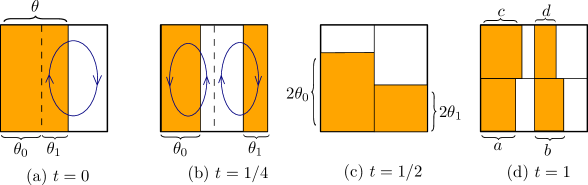
Figure 5. What $\rho(\cdot,t)$ would be at different times if $\psi^{\delta}$ were replaced by $\psi$ in the construction of the flow $u$.

For $t\in(0,\tfrac{1}{4}]$ let $u(x,y,t)=0$ when $x\in(0,\theta_{0}]$ and

$$u(x,y,t):=\nabla^{\perp}\left[2(1-\theta_{0})\psi^{\delta}\left(\frac{x-\theta_{0}}{1-\theta_{0}},y\right)\right]$$ (6.4)

when $x\in(\theta_{0},1)$. This flow, as well as $\rho(\cdot,0)$, is illustrated in Figure 5(a). Proposition 2.1(3) and symmetry show that if $\psi^{\delta}$ were replaced by $\psi$ here, then $\rho(\cdot,\tfrac{1}{4})$ would equal $\chi_{\{0<x<\theta_{0}\}}+\chi_{\{1-\theta_{1}<x<1\}}$, as illustrated in Figure 5(b). This is because the flow $\nabla^{\perp}[2\psi]$ rotates $Q$ by $180^{\circ}$ in time $\tfrac{1}{4}$. However, the factor $g^{\delta}$ in (6.2) limits us to only

$$\left\|\rho(\cdot,\tfrac{1}{4})-\chi_{\{0<x<\theta_{0}\}}-\chi_{\{1-\theta_{1}<x<1\}}\right\|_{1}\leq C\delta$$ (6.5)

for a new $C<\infty$. This is due to the area of the set of streamlines of $\psi$ whose distance from $\partial Q$ is $<\delta$ (which are the ones affected by $g^{\delta}$) being bounded by $C\delta$ (by $\nabla\varphi\in L^{\infty}$ and (A.5)). Notice also that $\theta_{0}\leq\tfrac{1}{2}$ and (6.3) show (with a new $C$)

$$\sup_{t\in(0,1/4]}\|\nabla u(\cdot,t)\|_{p}\leq C\delta^{-1+1/p}.$$ (6.6)

For $t\in(\tfrac{1}{4},\tfrac{1}{2}]$ let

$$u(x,y,t):=\nabla^{\perp}\left[\frac{(-1)^{\lfloor 2x\rfloor+1}}{2}\psi^{\delta}\left(\{2x\},y\right)\right],$$

with $\lfloor 2x\rfloor,\{2x\}$ the integer and fractional parts of $2x$, respectively. This flow is illustrated in Figure 5(b). Again (6.6) holds for $t\leq\tfrac{1}{2}$, and again, if $\psi^{\delta}$ were replaced by $\psi$ here and in (6.4), then $\rho(\cdot,\tfrac{1}{2})$ would equal

$$\chi_{(0,1/2)\times(0,2\theta_{0})}+\chi_{(1/2,1)\times(0,2\theta_{1})},$$

as shown in Figure 5(c). This is because the flow $\nabla^{\perp}\psi$ rotates $Q$ clockwise (and $\nabla^{\perp}[-\psi]$ rotates $Q$ counter-clockwise) by $90^{\circ}$ in time $\tfrac{1}{4}$, due to Proposition 2.1(3) and symmetry. However, as above, the extra factor $g^{\delta}$ means we only obtain (with a new $C$)

$$\left\|\rho(\cdot,\tfrac{1}{2})-\chi_{(0,1/2)\times(0,2\theta_{0})}-\chi_{(1/2,1)\times(0,2\theta_{1})}\right\|_{1}\leq C\delta.$$

For $t\in(\tfrac{1}{2},1]$ we run the same argument as for $t\in(0,\tfrac{1}{2}]$, but separately on the rectangles $(0,\tfrac{1}{2})\times(0,1)$ and $(\tfrac{1}{2},1)\times(0,1)$ instead of $Q$, and rotated by $90^{\circ}$ (so the first argument of the stream functions is either $2x$ or $2x-1$, instead of the second being $y$). The end result is

$$\left\|\rho(\cdot,1)-\chi_{(0,a)\times(0,1/2)}-\chi_{(1/2,1/2+b)\times(0,1/2)}-\chi_{(0,c)\times(1/2,1)}-\chi_{(1/2,1/2+d)\times(1/2,1)}\right\|_{1}\leq C\delta,$$

with a new $C$ and

$$a:=2^{1-2n}\sum_{i,j=0}^{2^{n-1}-1}\theta_{ij},\quad b:=2^{1-2n}\sum_{i=2^{n-1}}^{2^{n}-1}\sum_{j=0}^{2^{n-1}-1}\theta_{ij},\quad c:=2^{1-2n}\sum_{i=0}^{2^{n-1}-1}\sum_{j=2^{n-1}}^{2^{n}-1}\theta_{ij},\quad d:=2^{1-2n}\sum_{i,j=2^{n-1}}^{2^{n}-1}\theta_{ij}$$

(so $a+c=2\theta_{0}$ and $b+d=2\theta_{1}$). That is, $\rho(\cdot,1)$ is $C\delta$ close in $L^{1}(Q)$ to the function from Figure 5(d), which is the sum of characteristic functions of four rectangles, each being the intersection of one of the squares $Q_{100},Q_{101},Q_{110},Q_{111}$ with a half-plane with normal vector $(1,0)$, and each having area equal to $2^{-2n}$ times the sum of those $\theta_{ij}$ for which $Q_{nij}$ lies inside that square.

It is clear that a scaled version of this construction can be repeated for $t\in(1,2]$, separately on each square $Q_{100},Q_{101},Q_{110},Q_{111}$, with (6.6) still valid for these $t$ (because scaling of the stream functions is by a factor of 2 in space and $\tfrac{1}{4}$ in value) and at the expense of an additional $L^{1}$-norm error $\tfrac{1}{4}C\delta$ on each square. Continuing up to time $t=n$ and scale $2^{-n}$, we obtain $\|\rho(\cdot,n)-\sum_{i,j=0}^{2^{n}-1}\chi_{R_{ij}}\|_{1}\leq Cn\delta$, where $R_{ij}=(2^{-n}i,2^{-n}(i+\theta_{ij}))\times(2^{-n}j,2^{-n}(j+1))\subseteq Q_{nij}$ for any $i,j\in\{0,\dots,2^{n}-1\}$. So $S:=\bigcup_{i,j=0}^{2^{n}-1}R_{ij}$ and it now suffices to pick $\delta:=\tfrac{\kappa}{Cn}$.

The claim of the remark follows by replacing $\psi^{\delta}$ by $\psi$ in the proof. ∎

Proof of Corollary 1.7.

Let $\theta_{nij}:=2^{2n}|A\cap Q_{nij}|$ and consider the setting from the last sentence of the previous proof (i.e., $\kappa=0$ and $\psi$ in place of $\psi^{\delta}$) for any $n$ and with the $\theta_{ij}$ being the $\theta_{nij}$. Then the constructed flows for $n=n_{1}$ and $n=n_{2}$ obviously coincide for $t\in(0,\min\{n_{1},n_{2}\}]$. Thus there is a unique incompressible flow $u:Q\times{\mathbb{R}}^{+}\to{\mathbb{R}}^{2}$ satisfying the no-flow boundary condition which coincides with all these flows (for different $n$) on their time intervals of definition. One easily sees that $\sup_{t>0}\|u(\cdot,t)\|_{BV}<\infty$ so, in particular, (1.1) is well-posed.

Due to the nature of the scaling of the stream functions in the previous proof by a factor of $2^{k}$ in space and $2^{-2k}$ in value for $t\in(k,k+1]$ (relative to $t\in(0,1]$), we have

$$\sup_{t\in(k,k+1]}\|u(\cdot,t)\|_{\dot{W}^{s,p}}\leq C_{s,p}2^{(s-1)k}$$

for any $s<\tfrac{1}{p}$ and $k=0,1\dots$ (we need $s<\tfrac{1}{p}$ to make $u(\cdot,t)\in W^{s,p}$, since it is discontinuous along finitely many lines). Indeed, this follows from Lemma A.2 in the appendix (rather than from interpolation, as in the introduction, because the flows here do not belong to $W^{1,p}(Q)$). Scaling $u|_{(k,k+1]}$ in time by a factor of $(1-2^{s-1})^{-1}2^{(1-s)k}$ and multiplying it by the same factor creates an incompressible flow $\tilde{u}$ on $Q\times(0,1)$ such that

$$\sup_{t\in(0,1)}\|\tilde{u}(\cdot,t)\|_{\dot{W}^{s,p}}\leq C_{s,p}$$

(new $C_{s,p}$ equals old $C_{s,p}$ times $(1-2^{s-1})^{-1}$) and the solution to (1.1) with $\tilde{u}$ in place of $u$, and with $\rho(\cdot,0)=\chi_{\{0<x<|A|\}}$ satisfies $\fint_{Q_{nij}}\rho(x,y,1-2^{(s-1)n})\,dxdy=\theta_{nij}$ for all $n,i,j$. Because $A$ is measurable (so a.e. $(x,y)\in Q$ is its Lebesgue point), we obtain $\lim_{t\to 1}\|\rho(\cdot,t)-\chi_{A}\|_{1}=0$. ∎

Appendix: Properties of stream functions $\varphi,\varphi_{a},\varphi_{a,\delta}$ and two inequalities

Proof of Lemma 2.2.

The first two claims of (1) are obvious, and the other two follow from

$$\varphi_{x}(x,y)=4\cos(\pi x)\left(1+\dfrac{\sin(\pi x)}{\sin(\pi y)}\right)^{-2}$$ (A.1)

and a similar expression for $\varphi_{y}$.

To show (2), we start by taking another $x$-derivative of (A.1):

$$\varphi_{xx}(x,y)=-4\pi\sin(\pi x)\left(1+\dfrac{\sin(\pi x)}{\sin(\pi y)}\right)^{-2}-8\pi\cos^{2}(\pi x)\left(1+\dfrac{\sin(\pi x)}{\sin(\pi y)}\right)^{-2}\left(\sin(\pi x)+\sin(\pi y)\right)^{-1}.$$

Hence

$$|\varphi_{xx}(x,y)|\leq 4\pi+\frac{8\pi}{\sin(\pi x)+\sin(\pi y)}\leq 4\pi+\frac{8\pi}{\sqrt{2}\,d_{c}(x,y)}\leq\frac{40}{d_{c}(x,y)},$$

with $d_{c}$ the distance to the closest of the four corners of $Q$. Obviously, $\varphi_{yy}$ obeys the same bound due to symmetry. As for the cross term, taking the $y$ derivative of (A.1) gives

$$\varphi_{xy}(x,y)=8\pi\cos(\pi x)\cos(\pi y)\left(1+\dfrac{\sin(\pi x)}{\sin(\pi y)}\right)^{-1}\left(1+\dfrac{\sin(\pi y)}{\sin(\pi x)}\right)^{-1}\left(\sin(\pi x)+\sin(\pi y)\right)^{-1},$$

hence $|\varphi_{xy}(x,y)|\leq 20d_{c}(x,y)^{-1}.$ These estimates now show (2) because they yield

$$|\nabla^{2}\varphi(x,y)|\leq\frac{70}{d_{c}(x,y)}.$$ (A.2)

To show (3), first note that $\partial_{n}\varphi=-4$ on $\partial Q_{c}$ implies $T_{\varphi}(0)=1$. Consider the triangle $Q_{T}:=\{0<y<x<\tfrac{1}{2}\}$, and for $s\in(0,\tfrac{2}{\pi})$ let $\Gamma(s):=\{(x,y)\in Q_{T}:\varphi(x,y)=s\}$ (note that $0\leq\varphi\leq\tfrac{2}{\pi}$ on $Q$). By symmetry we have

$$T_{\varphi}(s)=8\int_{\Gamma(s)}\frac{1}{|\nabla\varphi|}d\sigma,$$

so with $|\Gamma(s)|$ the length of the curve $\Gamma(s)$,

$$T_{\varphi}(s)\leq 8|\Gamma(s)|\,\max_{\Gamma(s)}|\nabla\varphi|^{-1}.$$ (A.3)

Since $\varphi_{y}\geq\varphi_{x}>0$ on $Q_{T}$, the function of $x$ whose graph is $\Gamma(s)$ has slope between $-1$ and 0 on its domain $(b(s),\tfrac{1}{2})$, with $b(s):=\frac{1}{\pi}\arcsin\tfrac{\pi s}{2}$. Thus

$$|\Gamma(s)|\leq\sqrt{2}\left(\frac{1}{2}-\frac{1}{\pi}\arcsin\frac{\pi s}{2}\right)\quad(\leq 1),$$ (A.4)

for all $s$, and $\lim_{s\to 2/\pi}|\Gamma(s)|=0$. Moreover, on $\Gamma(s)$ we have $\sin(\pi x)\geq\sin(\pi y)$, so

$$\begin{split}|\nabla\varphi|^{-1}&\leq(\varphi_{y})^{-1}\leq\frac{1}{4\cos(\pi y)}\left(1+\frac{\sin(\pi y)}{\sin(\pi x)}\right)^{2}\leq\frac{1}{\cos(\pi b(s))}=\frac{1}{\sqrt{1-(\pi s/2)^{2}}}\end{split}$$ (A.5)

there. Combining (A.4) and (A.5) with (A.3) now gives

$$T_{\varphi}(s)\leq 8\sqrt{2}\,\frac{\frac{1}{2}-\frac{1}{\pi}\arcsin\frac{\pi s}{2}}{\sqrt{1-\left(\frac{\pi s}{2}\right)^{2}}}.$$

The fraction is bounded in $s\in[0,\frac{2}{\pi})$ away from $\tfrac{2}{\pi}$, and one can easily check that it converges to $\tfrac{1}{\pi}$ as $s\to\frac{2}{\pi}$. This proves (3).

It remains to prove (4). Let us first use the divergence theorem to find

$$\begin{split}T_{\varphi}(s)=\int_{\{\varphi=s\}}-n\cdot\frac{\nabla\varphi}{|\nabla\varphi|^{2}}d\sigma=\int_{\{\varphi>s\}}-\nabla\cdot\frac{\nabla\varphi}{|\nabla\varphi|^{2}}dxdy,\end{split}$$

with $n$ the outer unit normal vector to $\{\varphi>s\}$. This yields

$$T^{\prime}_{\varphi}(s)=\int_{\{\varphi=s\}}\frac{1}{|\nabla\varphi|}\nabla\cdot\frac{\nabla\varphi}{|\nabla\varphi|^{2}}d\sigma=\int_{\{\varphi=s\}}\left(\frac{\Delta\varphi}{|\nabla\varphi|^{3}}-2\frac{\nabla\varphi\cdot(\nabla^{2}\varphi\nabla\varphi)}{|\nabla\varphi|^{5}}\right)d\sigma$$ (A.6)

for $s\in(0,\tfrac{2}{\pi})$, so $T_{\varphi}$ is differentiable on $(0,\tfrac{2}{\pi})$. We also obtain

$$|T^{\prime}_{\varphi}(s)|\max_{\{\varphi=s\}}|\nabla\varphi|^{2}\leq 4\int_{\{\varphi=s\}}\frac{|\nabla^{2}\varphi|}{|\nabla\varphi|^{3}}d\sigma\left(\max_{\{\varphi=s\}}|\nabla\varphi|^{2}\right).$$ (A.7)

Recall that $\|\nabla\varphi\|_{\infty}<\infty$ by (1), and $|\nabla\varphi|^{-1}$ is easily seen to be uniformly bounded away from $(\tfrac{1}{2},\tfrac{1}{2})$ (where $s\approx\frac{2}{\pi}$). Since (A.2) shows that $|\nabla^{2}\varphi|$ is uniformly bounded away from the corners of $Q$ (where $s\approx 0$), we only need to bound the RHS of (A.7) near $s=0,\frac{2}{\pi}$.

For $s$ close to $\frac{2}{\pi}$ we have $|\nabla^{2}\varphi|\leq 200$ by (A.2), hence

$$|T^{\prime}_{\varphi}(s)|\max_{\{\varphi=s\}}|\nabla\varphi|^{2}\leq 800\int_{\{\varphi=s\}}\frac{1}{|\nabla\varphi|}d\sigma\frac{\max_{\{\varphi=s\}}|\nabla\varphi|^{2}}{\min_{\{\varphi=s\}}|\nabla\varphi|^{2}}=800T_{\varphi}(s)\frac{\max_{\{\varphi=s\}}|\nabla\varphi|^{2}}{\min_{\{\varphi=s\}}|\nabla\varphi|^{2}}.$$ (A.8)

The RHS is bounded near $\tfrac{2}{\pi}$ because $T_{\varphi}$ is bounded and the fraction is bounded near $\tfrac{2}{\pi}$. Indeed, by symmetry it suffices to show the latter with $\Gamma(s)$ in place of $\{\varphi=s\}$. We have

$$|\nabla\varphi|\geq\cos(\pi b(s))=\sin\left(\pi\left(\frac{1}{2}-b(s)\right)\right)$$

on $\Gamma(s)$ by (A.5). We also have $|\nabla\varphi|\leq\sqrt{2}\varphi_{y}\leq 4\sqrt{2}\cos(\pi y)$ on $\Gamma(s)$, as well as $y\geq b(s)-(\frac{1}{2}-b(s))=2b(s)-\tfrac{1}{2}$. The latter is because the curve starts at the point $(b(s),b(s))$ and its slope (as a function of $x$) is between 0 and $-1$ on the interval $(b(s),\tfrac{1}{2})$. It follows that

$$|\nabla\varphi|\leq 4\sqrt{2}\sin\left(2\pi\left(\frac{1}{2}-b(s)\right)\right)$$

on $\Gamma(s)$. Since $\frac{1}{2}-b(s)\approx 0$ for $s$ near $\frac{2}{\pi}$, the last fraction in (A.8) is bounded near $\tfrac{2}{\pi}$.

It remains to bound (A.7) for $s$ near $0$. Since $|\nabla\varphi|,|\nabla\varphi|^{-1}$ are both bounded near $\partial Q$ and the slope of $\Gamma(s)$ is between $0$ and $-1$, we obtain for some $C<\infty$,

$$\frac{1}{C}|T^{\prime}_{\varphi}(s)|\max_{\{\varphi=s\}}|\nabla\varphi|^{2}\leq\int_{\Gamma(s)}|\nabla^{2}\varphi|d\sigma\leq\int_{\Gamma(s)}\frac{70}{d_{c}(x,y)}d\sigma\leq\int_{b(s)}^{\frac{1}{2}}\frac{70\sqrt{2}}{x}dx\leq 100|\log b(s)|.$$

But $|\log b(s)|=|\log(\tfrac{1}{\pi}\arcsin\tfrac{\pi s}{2})|\leq|\log\tfrac{s}{2}|\leq 2|\log s|$ for $s$ near 0, so (4) is proved. ∎

Proof of Lemma 3.1.

Note that $\varphi_{a}=\varphi$ on $Q\setminus\{d_{P}<\tfrac{1}{5}\}\supseteq B_{3/10}(\frac{1}{2},\frac{1}{2})=:D$. All constants below may depend on $a\in(0,1]$.

The first, second, and fourth claim in (1) follow immediately from Lemma 2.2(1). We also obtain for $a>0$,

$$\begin{split}|\nabla\varphi_{a}(x,y)|&\leq|\nabla\varphi(x,y)|f(d_{P}(x,y))^{a}+\varphi(x,y)f(d_{P}(x,y))^{a-1}\|f^{\prime}\|_{\infty}|\nabla d_{P}(x,y)|\\ &\leq|\nabla\varphi(x,y)|\|f^{\prime}\|_{\infty}^{a}d_{P}(x,y)^{a}+\varphi(x,y)\|f^{\prime}\|_{\infty}^{a}d_{P}(x,y)^{a-1}\leq Cd_{P}(x,y)^{a}\end{split}$$ (A.9)

for some $C<\infty$, where in the last inequality we used $\varphi(x,y)\leq 2\pi d_{P}(x,y)$. So (1) is proved.

(2) is proved similarly: direct differentiation, together with $\varphi(x,y)\leq 2\pi d_{P}(x,y)$, (A.2), and $|\nabla^{2}d_{P}(x,y)|\leq d_{P}(x,y)^{-1}$ on $\{d_{P}<\tfrac{1}{5}\}$ yield for some $C<\infty$,

$$|\nabla^{2}\varphi_{a}(x,y)|\leq Cd_{P}(x,y)^{a-1}.$$ (A.10)

It remains to show (3) and (4). Since $\varphi_{a}=\varphi$ on $D$ (and $D$ fully contains the level sets $\{\varphi_{a}=s\}$ for all $s$ near $\tfrac{2}{\pi}$), all the claims hold when restricted to all $s$ near $\tfrac{2}{\pi}$, due to the same properties of $\varphi$. We therefore only need to consider $s$ away from $\tfrac{2}{\pi}$.

The claim in (3) about the level sets of $\varphi_{a}$ follows from the same statement for $\varphi$, and from positivity of the derivatives of $\varphi$ and $d_{P}$ in the direction $(\tfrac{1}{2},\tfrac{1}{2})-p$ inside each connected component of $\{d_{P}<\tfrac{1}{5}\}$, where $p$ is the unique point from $P$ belonging to that component. Also, since $s^{-2a/(a+1)}$ is integrable near 0 for $a\in(0,1)$ and $\nabla\varphi_{a}\in L^{\infty}(Q)$ for $a>0$, boundedness of $T_{\varphi_{a}}$ for $a\in(0,1)$ as well as (4) for $a\in(0,1]$ will follow if we show $\sup_{s\in(0,s_{0}]}s^{2a/(a+1)}|T_{\varphi_{a}}^{\prime}(s)|<\infty$ for $a\in(0,1]$, with $s_{0}:=\sup_{(x,y)\in Q\backslash D}\varphi(x,y)<\tfrac{2}{\pi}$.

For any $s\in(0,s_{0}]$, let $b_{a}(s)$ be the unique value such that $(b_{a}(s),b_{a}(s))\in\partial Q_{T}$ (with $Q_{T}$ from the proof of Lemma 2.2) and $\varphi_{a}(b_{a}(s),b_{a}(s))=s$. A direct computation yields $c^{\prime}s^{1/(a+1)}\leq b_{a}(s)\leq C^{\prime}s^{1/(a+1)}$ for some $c^{\prime},C^{\prime}\in(0,\infty)$. Due to (A.6) and symmetry we have

$$\begin{split}|T^{\prime}_{\varphi_{a}}(s)|\leq 32\int_{\{\varphi_{a}=s\}\cap Q_{T}}\frac{|\nabla^{2}\varphi_{a}|}{|\nabla\varphi_{a}|^{3}}d\sigma&=32\int_{b_{a}(s)}^{1/2}\frac{|\nabla^{2}\varphi_{a}(x,y_{a,s}(x))|}{|\nabla\varphi_{a}(x,y_{a,s}(x))|^{2}|(\varphi_{a})_{y}(x,y_{a,s}(x))|}dx\\ &\leq 32\int_{b_{a}(s)}^{1/2}\frac{|\nabla^{2}\varphi_{a}(x,y_{a,s}(x))|}{|(\varphi_{a})_{y}(x,y_{a,s}(x))|^{3}}dx,\end{split}$$ (A.11)

where $y_{a,s}(x)$ is such that $\varphi_{a}(x,y_{a,s}(x))=s$ and $(x,y_{a,s}(x))\in Q_{T}$. Its uniqueness is guaranteed by $(\varphi_{a})_{y}>0$ on $Q_{T}$, which holds because $\varphi,\partial_{y}\varphi$, and $f(d_{P}(x,y))$ are positive on $Q_{T}$, and $\partial_{y}[f(d_{P}(x,y))]\geq 0$ there. In fact, on $Q_{T}\cap\{\varphi<s_{0}\}$ we have for some $C<\infty$,

$$(\varphi_{a})_{y}(x,y)\geq\partial_{y}\varphi(x,y)f(d_{P}(x,y))^{a}\geq Cd_{P}(x,y)^{a}.$$

Combining this and (A.10) with (A.11) yields for $s\in(0,s_{0}]$ (with a new $C<\infty$),

$$\begin{split}\frac{1}{C}|T^{\prime}_{\varphi_{a}}(s)|&\leq\int_{b_{a}(s)}^{1/2}d_{P}(x,y_{a,s}(x))^{-1-2a}dx\\ &\leq\int_{b_{a}(s)}^{1/4}x^{-1-2a}dx+\int_{1/4}^{1/2-b_{a}(s)}\left(x-\frac{1}{2}\right)^{-1-2a}dx+\int_{1/2-b_{a}(s)}^{1/2}y_{a,s}(x)^{-1-2a}dx.\end{split}$$

The first two integrals are each bounded by $\tfrac{1}{2a}(c^{\prime})^{-2a}s^{-2a/(a+1)}$ (recall that $b_{a}(s)\geq c^{\prime}s^{1/(a+1)}$), as we need. For $x\in[\frac{1}{2}-b_{a}(s),\frac{1}{2}]$ and $s\in(0,s_{0}]$ we have (with $C:=\|\nabla\varphi\|_{\infty}\|f^{\prime}\|_{\infty}^{a}$)

$$\begin{split}s&=\varphi_{a}(x,y_{a,s}(x))\leq Cy_{a,s}(x)d_{P}(x,y_{a,s}(x))^{a}\leq C(C^{\prime})^{a}y_{a,s}(x)(s^{a/(a+1)}+y_{a,s}(x)^{a})\end{split}$$

because $\frac{1}{2}-x\leq b_{a}(s)\leq C^{\prime}s^{1/(a+1)}$. This gives $\max\{y_{a,s}(x)s^{a/(a+1)},y_{a,s}(x)^{a+1}\}\geq cs$ (with some $c\in(0,1]$), which implies $y_{a,s}(x)\geq cs^{1/(a+1)}$. This and $b_{a}(s)\leq C^{\prime}s^{1/(a+1)}$ show that the third integral is bounded by $C^{\prime}c^{-1-2a}s^{-2a/(a+1)}$ for $s\in(0,s_{0}]$. Hence we indeed get $\sup_{s\in(0,s_{0}]}s^{2a/(a+1)}|T_{\varphi_{a}}^{\prime}(s)|<\infty$ for $a\in(0,1]$, and we are done. ∎

Proof of Lemma 4.4.

Since $\varphi_{a,\delta}=\varphi_{a}$ on $D_{a,\delta}\cup\partial Q$, we only need to consider $s\in(0,\delta)$ in (1). Fix any $a\in(0,1)$, $\delta\in(0,\tfrac{1}{10})$, and $s\in(0,\delta)$. We also have $\varphi_{a,\delta}(x,y)=\varphi_{a}(x,y)$ when $d_{P}(x,y)\geq\tfrac{1}{5}d_{a,\delta}$, so their level sets coincide outside $B_{a,\delta}:=\{(x,y)\in Q:d_{P}(x,y)<\tfrac{1}{5}d_{a,\delta}\}$. (Recall that $d_{a,\delta}=c\delta^{1/(a+1)}$ for some $\delta$-independent $c>0$.) (1) now follows as the same claim for $\varphi_{a}$ in the proof of Lemma 3.1(3).

From Lemma 3.1(4) and $|\nabla\varphi|^{-1}$ being bounded except near the point $(\tfrac{1}{2},\tfrac{1}{2})$ (and hence $(\sup_{\{\varphi_{a}=s\}}|\nabla\varphi_{a}|^{2})^{-1}$ being bounded except near $s=\tfrac{2}{\pi}$) it follows that

$$\sup_{0<s\leq\delta<1/10}\delta^{-(1-a)/(a+1)}|T_{\varphi_{a}}(s)-T_{\varphi_{a}}(\delta)|<\infty.$$

It is therefore sufficient to show (2) with $T_{\varphi_{a}}(s)$ in place of $T_{\varphi_{a}}(\delta)$. The parts of the integrals defining $T_{\varphi_{a}}(s)$ and $T_{\varphi_{a,\delta}}(s)$ coincide outside $B_{a,\delta}$, so

$$T_{\varphi_{a,\delta}}(s)-T_{\varphi_{a}}(s)=\int_{\{\varphi_{a,\delta}=s\}\cap B_{a,\delta}}\frac{1}{|\nabla\varphi_{a,\delta}|}d\sigma-\int_{\{\varphi_{a}=s\}\cap B_{a,\delta}}\frac{1}{|\nabla\varphi_{a}|}d\sigma.$$

It therefore suffices to show

$$\sup_{0<s\leq\delta<1/10}\left(\delta^{(1-a)/(a+1)}\log\tfrac{2\delta}{s}\right)^{-1}\max\left\{\int_{\{\varphi_{a}=s\}\cap B_{a,\delta}}\frac{1}{|\nabla\varphi_{a}|}d\sigma,\int_{\{\varphi_{a,\delta}=s\}\cap B_{a,\delta}}\frac{1}{|\nabla\varphi_{a,\delta}|}d\sigma\right\}<\infty.$$ (A.12)

On $B_{a,\delta}$ we have $d_{P}\leq\tfrac{1}{10}$ (because $d_{a,\delta}<\tfrac{1}{2}$, which is due to $\varphi_{a}(\tfrac{1}{4},\tfrac{1}{4})=\tfrac{\sqrt{2}}{\pi}>\delta$), so

$$\varphi_{a}(x,y)=5^{a}\varphi(x,y)d_{P}(x,y)^{a}\qquad\text{and}\qquad\varphi_{a,\delta}(x,y)=5^{a}\varphi(x,y)d_{P}(x,y)^{a}f\left(\frac{d_{P}(x,y)}{d_{a,\delta}}\right)^{1-a}$$

there. Also, $B_{a,\delta}$ has 8 connected components, but the following analysis is essentially the same in each of them. We will therefore only consider the one near the origin (or rather one half of it, due to symmetry). So let $B^{\prime}:=B_{d_{a,\delta}/5}(0,0)\cap\{0<y<x\}$.

On $B^{\prime}$ we have $\varphi_{x},\varphi_{y},(d_{P})_{x},(d_{P})_{y}>0$, which together with $f^{\prime}\geq 0$ shows that (with the usual $\sim$ notation, where constants depend on $a$ but not on $\delta,s$)

$$|\nabla\varphi_{a}|\sim(\varphi_{a})_{x}+(\varphi_{a})_{y}\qquad\text{and}\qquad|\nabla\varphi_{a,\delta}|\sim(\varphi_{a,\delta})_{x}+(\varphi_{a,\delta})_{y}$$ (A.13)

and also that the curves $\{\varphi_{a}=s\}\cap B^{\prime}$ and $\{\varphi_{a,\delta}=s\}\cap B^{\prime}$ are graphs of decreasing functions of $x$. Those graphs start at some points $(b_{a}(s),b_{a}(s))$ and $(b_{a,\delta}(s),b_{a,\delta}(s))$ (the former being from the proof of Lemma 3.1). Since $\varphi(x,y)\sim y$ and $d_{P}(x,y)\sim x$ on $B^{\prime}$, and $f(r)\sim r$ on $(0,1)$, we obtain (using also $d_{a,\delta}=c\delta^{1/(a+1)}$)

$$b_{a}(s)\sim s^{1/(a+1)}\qquad\text{and}\qquad b_{a,\delta}(s)\sim\delta^{(1-a)/(2a+2)}s^{1/2}.$$ (A.14)

Since on $B^{\prime}$ we also have $0\leq\varphi_{x}\leq\varphi_{y}\sim 1$ and $0\leq(d_{P})_{y}\leq(d_{P})_{x}\sim 1$, it follows that

$$|\nabla\varphi_{a}(x,y)|\sim x^{a}\qquad\text{and}\qquad|\nabla\varphi_{a,\delta}(x,y)|\sim\delta^{-(1-a)/(a+1)}x$$

on $B^{\prime}$. From this and (A.14) we obtain that the first integral in (A.12), with $B_{a,\delta}$ replaced by $B^{\prime}$, is bounded above by a constant times

$$\int_{b_{a}(s)}^{d_{a,\delta}}x^{-a}(1+|h^{\prime}(x)|)dx\leq\int_{b_{a}(s)}^{d_{a,\delta}}x^{-a}dx+b_{a}(s)^{-a}b_{a}(s)\lesssim\delta^{(1-a)/(a+1)},$$

with $h$ the decreasing function whose graph is $\{\varphi_{a}=s\}\cap B^{\prime}$. By the same argument (and also using $\tfrac{1}{1+a}-\tfrac{1-a}{2a+2}=\tfrac{1}{2}$), the second integral is bounded above by a constant times

$$\int_{b_{a,\delta}(s)}^{d_{a,\delta}}\delta^{(1-a)/(a+1)}x^{-1}dx+\delta^{(1-a)/(a+1)}b_{a,\delta}(s)^{-1}b_{a,\delta}(s)\lesssim\delta^{(1-a)/(a+1)}(1+\log\tfrac{\delta}{s}).$$

The same bounds are obtained for the integrals from (A.12) over the remaining parts of $B_{a,\delta}$ (the 4 connected components in the corners of $Q$ are divided into 2 parts each, the other 4 connected components into 4 parts each). This proves (A.12), and thus (2). ∎

Lemma A.1.

There is $c>0$ such that for any $s\in[0,1]$ and $\kappa,\varepsilon\in(0,\tfrac{1}{2}]$, a function $f\in L^{\infty}(Q)$ is $\kappa$-mixed to scale $\varepsilon$ whenever $\|f\|_{{H}^{-s}}\leq c\kappa^{3s/2}\varepsilon^{1+s}\|f\|_{\infty}$.

Proof.

Let us consider the same test function $g:\mathbb{R}^{2}\to[0,1]$ as in [8, Lemma 2.3], smooth and satisfying $g=1$ on $B(0,\varepsilon)$, $g=0$ on ${\mathbb{R}}^{2}\setminus B(0,(1+\frac{\kappa}{20})\varepsilon)$, and $\|\nabla g\|_{\infty}\leq\tfrac{40}{\kappa\varepsilon}$. Elementary computations yield $\|g\|_{2}\leq C_{1}\varepsilon$ and $\|g\|_{\dot{H}^{1}}\leq C_{1}\kappa^{-1/2}$ for some $C_{1}<\infty$. Interpolation then gives us $\|g\|_{\dot{H}^{s}}\leq C_{1}\kappa^{-s/2}\varepsilon^{1-s}$ for $s\in[0,1]$. We thus have for any $x\in Q$ such that $d(x,\partial Q)\geq 2\varepsilon$ (so that $g(\cdot-x)$ is supported on $Q$),

$$\left|\int_{Q}f(y)g(y-x)dy\right|\leq\|f\|_{{H}^{-s}}\|g\|_{\dot{H}^{s}}\leq C_{1}c\kappa\varepsilon^{2}\|f\|_{\infty},$$

which gives

$$\left|\fint_{B_{\varepsilon}(x)}f(y)dy\right|\leq\frac{1}{\pi\varepsilon^{2}}\left(\left|\int_{Q}f(y)g(y-x)dy\right|+\frac{3\pi\kappa\varepsilon^{2}}{20}\|f\|_{\infty}\right)\leq\left(\frac{C_{1}c}{\pi}+\frac{3}{20}\right)\kappa\|f\|_{\infty}.$$ (A.15)

For $x\in Q$ such that $d(x,\partial Q)<2\varepsilon$ we instead use the test function $g(\cdot-x)h(\cdot)$, where $h(y)=1$ when $d(y,\partial Q)\geq\frac{\kappa\varepsilon}{20}$, $h=0$ on ${\mathbb{R}}^{2}\setminus Q$ and $\|\nabla h\|_{\infty}\leq\frac{40}{\kappa\varepsilon}$. An identical argument as above yields $\|g(\cdot-x)h(\cdot)\|_{\dot{H}^{s}}\leq C_{2}\kappa^{-s/2}\varepsilon^{1-s}$ for some $C_{2}<\infty$ and all $s\in[0,1]$. Similarly to (A.15) we also obtain

$$\left|\fint_{B_{\varepsilon}(x)\cap Q}f(y)dy\right|\leq\left(\frac{4C_{2}c}{\pi}+\frac{12}{20}\right)\kappa\|f\|_{\infty}$$ (A.16)

because $|B_{\varepsilon}(x)\cap Q|\geq\tfrac{\pi}{4}\varepsilon^{2}$. Choosing $c:=\tfrac{\pi}{10}\max\{C_{1},C_{2}\}^{-1}$ finishes the proof. ∎

Lemma A.2.

Let $p\in[1,\infty)$, $s\in(0,\tfrac{1}{p})$, and $n\geq 0$. Assume that a family of functions $\{f_{ij}\}_{i,j=0}^{2^{n}-1}$ on $Q$ satisfies $\|f_{ij}\|_{W^{s,p}}\leq 1$ and $\|f_{ij}\|_{\infty}\leq 1$ for any $i,j\in\{0,\ldots,2^{n}-1\}$. Let $f:Q\to\mathbb{R}$ be defined on each $Q_{nij}$ by

$$f(x)=2^{-n}f_{ij}(2^{n}x-(i,j)).$$

Then we have $\|f\|_{W^{s,p}}\leq C_{s,p}\,2^{-(1-s)n}$ for some $C_{s,p}>0$ which depends only on $s,p$.

Proof.

Since $s\in(0,1)$ and $Q\subseteq\mathbb{R}^{2}$, the fractional Sobolev norm can equivalently be defined by (see, e.g., [13])

$$\|f\|_{W^{s,p}}=\Bigg{(}\int_{Q}|f|^{p}dx+\underbrace{\int_{Q^{2}}\frac{|f(x)-f(y)|^{p}}{|x-y|^{2+sp}}dxdy}_{=:I[f]}\Bigg{)}^{1/p}.$$

Obviously $\|f\|_{p}\leq 2^{-n}$, so it is sufficient to show $I[f]\leq C_{s,p}2^{-(1-s)np}$. This would follow from

$$\int_{Q_{nij}\times Q}\frac{|f(x)-f(y)|^{p}}{|x-y|^{2+sp}}dxdy\leq C_{s,p}\,2^{-2n-(1-s)np}$$ (A.17)

for any $i,j\in\{0,\ldots,2^{n}-1\}$, which we shall now prove.

Since $I[f_{ij}]\leq 1$ for any $i,j$ by the hypothesis, we have

$$\int_{Q_{nij}^{2}}\frac{|f(x)-f(y)|^{p}}{|x-y|^{2+sp}}dxdy=2^{-2n-(1-s)np}I[f_{ij}]\leq 2^{-2n-(1-s)np}.$$ (A.18)

Also, for some $C_{s,p}<\infty$ and any $x\in Q_{nij}$ we have using $\|f\|_{L^{\infty}(Q)}\leq 2^{-n}$,

$$\int_{Q\setminus Q_{nij}}\frac{|f(x)-f(y)|^{p}}{|x-y|^{2+sp}}dy\leq\int_{d(x,\partial Q_{nij})}^{\sqrt{2}}\frac{(2\|f\|_{\infty})^{p}}{r^{2+sp}}2\pi rdr\leq C_{s,p}\,2^{-np}d(x,\partial Q_{nij})^{-sp}.$$

Integrating this in $x\in Q_{nij}$ and using $sp<1$ gives (with a new $C_{s,p}$)

$$\int_{Q_{nij}\times(Q\setminus Q_{nij})}\frac{|f(x)-f(y)|^{p}}{|x-y|^{2+sp}}dxdy\leq C_{s,p}\,2^{-np}\int_{Q_{nij}}d(x,\partial Q_{nij})^{-sp}dx\leq C_{s,p}\,2^{-2n-(1-s)np}.$$

Adding this to (A.18) yields (A.17). ∎

References

- [1] G. Alberti, G. Crippa, and A. Mazzucato, Exponential self-similar mixing and loss of regularity for continuity equations, preprint, 2014. arXiv:1407.2631
- [2] Y. Brenier, F. Otto, and C. Seis. Upper bounds on the coarsening rates in demixing binary viscous fluids. SIAM J. Math. Anal., 43:114–134, 2011.
- [3] A. Bressan. A lemma and a conjecture on the cost of rearrangements. Rend. Sem. Mat. Univ. Padova, 110:97–102, 2003.
- [4] A. Bressan. Prize offered for the solution of a problem on mixing flows. http://www.math.psu.edu/bressan/PSPDF/prize1.pdf, 2006.
- [5] P. Constantin, A. Kiselev, L. Ryzhik, and A. Zlatoš. Diffusion and mixing in fluid flow. Ann. of Math. (2), 168(2):643–674, 2008.
- [6] G. Crippa and C. De Lellis. Estimates and regularity results for the DiPerna-Lions flow. J. Reine Angew. Math., 616:15–46, 2008.
- [7] C. R. Doering and J.-L. Thiffeault. Multiscale mixing efficiencies for steady sources. Phys. Rev. E, 74 (2), 025301(R), August 2006.
- [8] G. Iyer, A. Kiselev, and X. Xu. Lower bounds on the mix norm of passive scalars advected by incompressible enstrophy-constrained flows. Nonlinearity, 27(5):973–985, 2014.
- [9] Z. Lin, J. L. Thiffeault, and C. R. Doering. Optimal stirring strategies for passive scalar mixing. J. Fluid Mech., 675:465–476, 2011.
- [10] E. Lunasin, Z. Lin, A. Novikov, A. Mazzucato, and C. R. Doering. Optimal mixing and optimal stirring for fixed energy, fixed power, or fixed palenstrophy flows. J. Math. Phys., 53(11):115611, 15, 2012.
- [11] G. Mathew, I. Mezić, and L. Petzold. A multiscale measure for mixing. Physica D, 211(1-2):23–46, 2005.
- [12] V. Maz’ya, Sobolev Spaces. With Applications to Elliptic Partial Differential Equations, 2nd, revised and augmented ed., Springer, Berlin, 2011.
- [13] E. Di Nezza, G. Palatucci, and E. Valdinoci. Hitchhiker’s guide to the fractional Sobolev spaces, Bull. Sci. math., 136(5):521–573, 2012.
- [14] F. Otto, C. Seis, and D. Slepčev. Crossover of the coarsening rates in demixing of binary viscous liquids. Commun. Math. Sci. 11:441–464, 2013.
- [15] C. Seis. Maximal mixing by incompressible fluid flows. Nonlinearity, 26(12):3279–3289, 2013.
- [16] D. Slepčev. Coarsening in nonlocal interfacial systems. SIAM J. Math. Anal., 40(3):1029–1048, 2008.
- [17] T. A. Shaw, J.-L. Thiffeault, and C. R. Doering. Stirring up trouble: multi-scale mixing measures for steady scalar sources. Phys. D, 231(2):143–164, 2007.
- [18] J.-L. Thiffeault. Using multiscale norms to quantify mixing and transport. Nonlinearity, 25(2):R1–R44, 2012.
- [19] J.-L. Thiffeault, C. R. Doering, and J. D. Gibbon. A bound on mixing efficiency for the advection-diffusion equation. J. Fluid Mech., 521:105–114, 2004.