Accessing topological order in fractionalized liquids with gapped edges

Abstract

We consider manifestations of topological order in time-reversal-symmetric fractional topological liquids (TRS-FTLs), defined on planar surfaces with holes. We derive a formula for the topological ground state degeneracy of such a TRS-FTL, which applies to cases where the edge modes on each boundary are fully gapped by appropriate backscattering terms. The degeneracy is exact in the limit of infinite system size, and is given by $q^{N^{\,}_{\mathrm{h}}}$, where $N^{\,}_{\mathrm{h}}$ is the number of holes and $q$ is an integer that is determined by the topological field theory. When the degeneracy is lifted by finite-size effects, the holes realize a system of $N^{\,}_{\mathrm{h}}$ coupled spin-like $q$-state degrees of freedom. In particular, we provide examples where $\mathbb{Z}^{\,}_{q}$ quantum clock models are realized on the low-energy manifold of states. We also investigate the possibility of measuring the topological ground state degeneracy with calorimetry, and briefly revisit the notion of topological order in $s$-wave BCS superconductors.

I Introduction

The robust ground state degeneracy (GSD) that arises in topologically ordered systems Wen (1989); Wen and Niu (1990); Wen (1991) has been an object of intense study over the past quarter-century. Interest in such states of matter has been motivated in large part by the desire to access quasiparticles with non-Abelian statistics, whose nontrivial braiding could be used as a platform for quantum computation. Nayak et al. (2008) Nevertheless, to date there has been no definitive experimental proof that such non-Abelian quasiparticles exist, nor has there been any direct observation of topological GSD.

There have been several theoretical proposals for the experimental detection of topological degeneracy. One set of proposals for the (putative) non-Abelian $\nu=5/2$ quantum Hall state focuses on measuring the contribution of the GSD to the electronic portion of the entropy at low temperatures. Observable signatures of this contribution include the thermopower Yang and Halperin (2009); Barlas and Yang (2012) and the temperature dependence of the electrochemical potential and orbital magnetization. Cooper and Stern (2009) The thermopower has been measured on several occasions Chickering et al. (2010, 2013) with no conclusive signatures. Abelian fractional quantum Hall (FQH) states Wen and Zee (1992) are also topologically ordered, but the bulk GSD in these systems is only accessible on closed surfaces (e.g., the torus). This is unnatural for experiments, which are confined to finite planar systems, although a recent proposal Barkeshli et al. (2014) suggests a transport measurement in a bilayer FQH system that avoids this handicap by effectively altering the topology of the system.

In this paper, we propose that time-reversal-symmetric fractional topological liquids (FTLs) may constitute a promising alternative platform for realizing the topological GSD in experimentally accessible geometries. FTLs with time-reversal symmetry (TRS) have an effective description in terms of doubled Chern-Simons (CS), or so-called BF, theories. Freedman et al. (2004) Examples of time-reversal-symmetric FTLs with topological order include fractional quantum spin Hall systems, Kane and Mele (2005a, b); Bernevig and Zhang (2006) certain spin liquids, Scharfenberger et al. (2011) Kitaev’s toric code, Kitaev (2003) and even the $s$-wave BCS superconductor. Wen (1991); Hansson et al. (2004) In the present work we emphasize FTLs whose edge states in planar geometries can be completely gapped without breaking TRS, which is possible when certain criteria are satisfied. Levin and Stern (2009); Neupert et al. (2011) In these cases, the degenerate ground state manifold is well separated from excited states and the GSD on punctured planar surfaces is accessible experimentally.

Our program for this paper is as follows. We first derive a formula for the GSD of a doubled CS theory defined on a plane with $N^{\,}_{\mathrm{h}}$ holes, in cases where all helical edge modes are gapped by appropriate backscattering terms. This topological degeneracy increases exponentially with the number of holes, and is exact in the limit where all holes are infinitely large and infinitely far apart. We then consider finite-sized systems, where the degeneracy is split exponentially by quasiparticle tunneling processes. In this setting, we argue that the holes themselves realize an effective spin-like system, whose Hilbert space consists of what was formerly the degenerate ground state manifold. We then examine calorimetry as a possible experimental probe of the degeneracy. We argue that, for suitable materials, the contribution of the GSD to the low-temperature heat capacity could be observed experimentally, even in the presence of the expected phononic and electronic backgrounds. Finally, we also briefly revisit the notion of topological order in $s$-wave superconductors, which was suggested by WenWen (1991) and investigated in detail by Hansson et al. in Ref. Hansson et al., 2004. We argue that, for a thin-film superconductor with (3+1)-dimensional electromagnetism, there is indeed a ground state degeneracy, which is related to flux quantization. However, this degeneracy is lifted in a power-law fashion, rather than exponentially, and is therefore not topological in the canonical sense of Refs. Wen, 1989–Wen, 1991.

II The topological degeneracy

In this section we derive a formula for the ground state degeneracy of a TRS-FTL with appropriately gapped edges. We begin with some preliminary information before moving on to the derivation.

II.1 Definitions and notation

A general time-reversal-symmetric doubled Chern-Simons theory in (2+1)-dimensional space and time has the form Neupert et al. (2011)

$$\mathcal{L}^{\,}_{\mathrm{CS}} \,\raisebox{0.85pt}{.}\raisebox{2.85pt}{.}\!\!=\,\frac{1}{4\pi}\,K^{\,}_{\mathsf{ij}}\,\epsilon^{\mu\nu\rho}\,a^{\mathsf{i}}_{\mu}\,\partial^{\,}_{\nu}\,a^{\mathsf{j}}_{\rho}+\frac{e}{2\pi}\,Q^{\,}_{\mathsf{i}}\,\epsilon^{\mu\nu\rho}\,A^{\,}_{\mu}\,\partial^{\,}_{\nu}\,a^{\mathsf{i}}_{\rho},$$ (1a)

where $$\mathsf{i},\mathsf{j}=1,\ldots,2N \mu,\nu,\rho=0,1,2 2N\times 2N K^{\,}_{\mathsf{ij}} \epsilon^{\mu\nu\rho} \epsilon^{012}=1 A^{\,}_{\mu} \bm{Q} a^{\mathsf{i}}_{\mu} e N 2N\times 2N K$$, , and summation on repeated indices is implied. Here, the matrix is symmetric, invertible, and integer-valued. The fully antisymmetric Levi-Civita tensor appears with the convention . The components of the electromagnetic gauge potential are restricted to (2+1)-dimensional space and time, and the vector has integer entries that measure the charges of the various CS fields in units of the electron charge . The theory contains Kramers pairs of CS fields, which transform into one another under the operation of time-reversal. We will therefore be particularly interested in scenarios where the matrix has the following block form, which is consistent with TRS, as was shown in Ref. Neupert et al., 2011,

$$K\,\raisebox{0.85pt}{.}\raisebox{2.85pt}{.}\!\!=\,\begin{pmatrix}\kappa&\Delta\\ \Delta^{\mathsf{T}}&-\kappa\end{pmatrix},$$ (1b)

where the $$N\times N \kappa=\kappa^{\mathsf{T}} \Delta=-\Delta^{\mathsf{T}}$$ matrices and . TRS further imposes that the charge vector possess the block form (see Ref. Neupert et al., 2011)

$$\bm{Q}\,\raisebox{0.85pt}{.}\raisebox{2.85pt}{.}\!\!=\,\begin{pmatrix}\varrho\\ \varrho\end{pmatrix}.$$ (1c)

The theory (1) can also be re-expressed in terms of an equivalent BF theory Santos et al. (2011) by defining the linear transformation $\tilde{a}^{\mathsf{i}}_{\mu}\,\raisebox{0.85pt}{.}\raisebox{2.85pt}{.}\!\!=\,R^{\,}_{\mathsf{ij}}\,a^{\mathsf{j}}_{\mu}$, where

$$R\,\raisebox{0.85pt}{.}\raisebox{2.85pt}{.}\!\!=\,\begin{pmatrix}\mathbbm{1}&\mathbbm{1}\\ \frac{\mathbbm{1}}{2}&-\frac{\mathbbm{1}}{2}\end{pmatrix},$$ (2a)

with $$\mathbbm{1} N\times N K$$ the identity matrix. This linear transformation induces the -matrix and charge vector

$$\tilde{K} \,\raisebox{0.85pt}{.}\raisebox{2.85pt}{.}\!\!=\,(R^{-1})^{\mathsf{T}}\,K\,R^{-1}=\begin{pmatrix}0&\varkappa\\ \varkappa^{\mathsf{T}}&0\end{pmatrix},$$ (2b)

$$\varkappa \,\raisebox{0.85pt}{.}\raisebox{2.85pt}{.}\!\!=\,\kappa-\Delta,$$ (2c)

$$\tilde{\bm{Q}} \,\raisebox{0.85pt}{.}\raisebox{2.85pt}{.}\!\!=\,(R^{-1})^{\mathsf{T}}\,\bm{Q}=\begin{pmatrix}\varrho\\ 0\end{pmatrix}.$$ (2d)

Note that the transformation (2a) preserves $\det\,K$ [c.f. Eq. (2d)].

When defined on a manifold with boundary, the CS theory (1a) has an associated theory of $2N$ chiral bosons $\phi^{\,}_{\mathsf{i}}$ at the edge. In the most generic case, the boundary of the system consists of a disjoint union of an arbitrary number of edges, each with a Lagrangian density of the form (in the absence of the gauge field $A^{\,}_{\mu}$) Neupert et al. (2011)

$$\mathcal{L}^{\,}_{\mathrm{E}} =\frac{1}{4\pi}\,\left(K^{\,}_{\mathsf{ij}}\,\partial^{\,}_{t}\,\phi^{\,}_{\mathsf{i}}\,\partial^{\,}_{x}\,\phi^{\,}_{\mathsf{j}}-V^{\,}_{\mathsf{ij}}\,\partial^{\,}_{x}\,\phi^{\,}_{\mathsf{i}}\,\partial^{\,}_{x}\,\phi^{\,}_{\mathsf{j}}\right)+\mathcal{L}^{\,}_{\mathrm{T}},$$ (3)

where $K^{\,}_{\mathsf{ij}}$ is the same $2N\times 2N$ matrix as before and the positive-definite, real-valued, symmetric matrix $V^{\,}_{\mathsf{ij}}$ encodes non-universal information specific to a particular edge. The Lagrangian density $\mathcal{L}^{\,}_{\mathrm{T}}$ generically contains all inter-channel tunneling operators,

$$\mathcal{L}^{\,}_{\mathrm{T}}\,\raisebox{0.85pt}{.}\raisebox{2.85pt}{.}\!\!=\,\sum_{\bm{T}\in\mathbb{L}}U^{\,}_{\bm{T}}(x)\,\cos\Big{(}\bm{T}^{\mathsf{T}}\,K\,\bm{\phi}(x)+\zeta^{\,}_{\bm{T}}(x)\Big{)},$$ (4)

where $\bm{T}$ is a $2N$-dimenisonal integer vector, $\bm{\phi}^{\mathsf{T}}=(\phi^{\,}_{1}\ \ldots\ \phi^{\,}_{2N})$, and $\mathbb{L}$ is the set of all tunneling vectors $\bm{T}$ allowed by TRS and charge conservation (if it holds). The real-valued functions $U^{\,}_{\bm{T}}(x)$ and $\zeta^{\,}_{\bm{T}}(x)$ encode information about disorder at the edge and are further constrained to be consistent with TRS (see Ref. Neupert et al., 2011). When TRS is imposed, a necessary and sufficient condition for gapping out the bosonic modes in the edge theory (3) is the existence of $N$ $2N$-dimensional vectors $\bm{T}^{\,}_{i}\in\mathbb{L}$ satisfying Neupert et al. (2011); Haldane (1995)

$$\bm{T}^{\mathsf{T}}_{i}\,\bm{Q}=0,\quad\forall\ i\indent\text{(charge conservation)},$$ (5a)

$$\bm{T}^{\mathsf{T}}_{i}\,K\,\bm{T}^{\,}_{j}=0,\quad\forall\ i,j\indent\text{(Haldane criterion)}.$$ (5b)

Strictly speaking, the criterion (5a) need not hold in a general system, such as (for example) in the case of a superconductor. In this case, one replaces charge conservation with charge conservation mod 2 (i.e., conservation of fermion parity), so that $\bm{T}^{\mathsf{T}}_{i}\,\bm{Q}$ is only constrained to be even. In the next section, we will focus on cases where the criteria (5) are satisfied.

II.2 Gauge invariance in a system with gapped edges

The need for the edge theory (3) arises from the failure of gauge invariance in Chern-Simons theories on manifolds with boundary. For non-chiral Chern-Simons theories, like those of the form (1), the ability to gap out the edge states necessitates an alternate route to gauge invariance, as we now show. For simplicity, we will work on the disk, although analogous results hold for manifolds with multiple disconnected boundaries.

To proceed, we rewrite the Lagrangian density (1a), in the absence of the electromagnetic gauge potential $A^{\,}_{\mu}$ (which we ignore hereafter), in terms of two separate sets of $N$ CS fields $\alpha^{\mathtt{i}}$ and $\beta^{\mathtt{i}}$,

$$\begin{split}\mathcal{L}^{\,}_{\mathrm{CS}}=&\,\frac{\epsilon^{\mu\nu\rho}}{4\pi}\,\left[\kappa^{\,}_{\mathtt{ij}}\,\left(\alpha^{\mathtt{i}}_{\mu}\,\partial^{\,}_{\nu}\,\alpha^{\mathtt{j}}_{\rho}-\beta^{\mathtt{i}}_{\mu}\,\partial^{\,}_{\nu}\,\beta^{\mathtt{j}}_{\rho}\right)\right.\\ &\,\left.+\Delta^{\,}_{\mathtt{ij}}\left(\alpha^{\mathtt{i}}_{\mu}\,\partial^{\,}_{\nu}\,\beta^{\mathtt{j}}_{\rho}-\beta^{\mathtt{i}}_{\mu}\,\partial^{\,}_{\nu}\,\alpha^{\mathtt{j}}_{\rho}\right)\right].\end{split}$$ (6)

Here, ${\mathtt{i}},\mathtt{j}\in\{1,\ldots,N\}$, and the “new” CS fields are defined as $\alpha^{\mathtt{i}}_{\mu}(\bm{x},t)\equiv a^{\mathtt{i}}_{\mu}(\bm{x},t)$ and $\beta^{\mathtt{i}}_{\mu}(\bm{x},t)\equiv a^{{\mathtt{i}}+N}_{\mu}(\bm{x},t)$. We define the CS action on the disk $D$ to be

$$S^{\,}_{\mathrm{CS}}\,\raisebox{0.85pt}{.}\raisebox{2.85pt}{.}\!\!=\,\int\limits\mathrm{d}t\int\limits_{D}\mathrm{d}^{2}x\,\mathcal{L}^{\,}_{\mathrm{CS}}(\bm{x},t).$$ (7)

Its transformation law under any local gauge transformation of the form

$$\alpha^{\mathtt{i}}_{\mu}\mapsto\alpha^{\mathtt{i}}_{\mu}+\partial^{\,}_{\mu}\,\chi^{\mathtt{i}}_{\alpha},\qquad\beta^{\mathtt{i}}_{\mu}\mapsto\beta^{\mathtt{i}}_{\mu}+\partial^{\,}_{\mu}\,\chi^{\mathtt{i}}_{\beta},$$ (8a)

where $$\mathtt{i}=1,\ldots,N \chi^{\mathtt{i}}_{\alpha} \chi^{\mathtt{i}}_{\beta}$$ and and are real-valued scalar fields, is

$$S^{\,}_{\mathrm{CS}}\mapsto S^{\,}_{\mathrm{CS}}+\delta S^{\,}_{\mathrm{CS}}$$ (8b)

with the boundary contribution

$$\delta S^{\,}_{\mathrm{CS}}\,\raisebox{0.85pt}{.}\raisebox{2.85pt}{.}\!\!=\, \,\int\limits\mathrm{d}t\oint\limits_{\partial D}\mathrm{d}x^{\,}_{\mu}\,\frac{\epsilon^{\mu\nu\rho}}{4\pi}\,\left[\kappa^{\,}_{\mathtt{ij}}\left(\chi^{\mathtt{i}}_{\alpha}\,\partial^{\,}_{\nu}\,\alpha^{\mathtt{j}}_{\rho}-\chi^{\mathtt{i}}_{\beta}\,\partial^{\,}_{\nu}\,\beta^{\mathtt{j}}_{\rho}\right)\right.$$

$$\,\left.+\Delta^{\,}_{\mathtt{ij}}\left(\chi^{\mathtt{i}}_{\alpha}\,\partial^{\,}_{\nu}\,\beta^{\mathtt{j}}_{\rho}-\chi^{\mathtt{i}}_{\beta}\,\partial^{\,}_{\nu}\,\alpha^{\mathtt{j}}_{\rho}\right)\right].$$ (8c)

Here, the boundary $\partial D$ of the disk $D$ is the circle $S^{1}$, and $\mathrm{d}x^{\,}_{\mu}\,\raisebox{0.85pt}{.}\raisebox{2.85pt}{.}\!\!=\,\epsilon^{\,}_{\mu 0\sigma}\,\mathrm{d}\ell^{\sigma}$, with $\mathrm{d}\ell^{\sigma}$ the line element along the boundary.

There are two ways to impose gauge invariance in the doubled Chern-Simons theory $S^{\,}_{\mathrm{CS}}$. On the one hand, if the criteria (5) do not hold, we must demand that there exist a gapless edge theory with an action $S^{\,}_{E}$ that transforms as $S^{\,}_{\mathrm{E}}\mapsto S^{\,}_{\mathrm{E}}-\delta S^{\,}_{\mathrm{CS}}$, so that the total action $S^{\,}_{\mathrm{CS}}+S^{\,}_{\mathrm{E}}$ is gauge invariant. On the other hand, if the criteria (5) hold, then the edge fields $\phi^{\,}_{\mathsf{i}}$ become pinned to the classical minima of the cosine potentials in $\mathcal{L}^{\,}_{\mathrm{T}}$ for large $|U^{\,}_{\bm{T}}(x)|$, and are then no longer dynamical degrees of freedom. In this case, gauge invariance can be achieved by demanding that the anomalous term $\delta S^{\,}_{\mathrm{CS}}=0$ identically. The latter option can be accomplished by imposing the boundary conditions

$$\chi^{\mathtt{i}}_{\alpha}|^{\,}_{\partial D}=T^{\,}_{\mathtt{ij}}\,\chi^{\mathtt{j}}_{\beta}|^{\,}_{\partial D},\qquad\alpha^{\mathtt{i}}_{\mu}|^{\,}_{\partial D}=T^{\,}_{\mathtt{ij}}\,\beta^{\mathtt{j}}_{\mu}|^{\,}_{\partial D},$$ (9a)

for all $$\mathtt{i}=1,\dots,N N\times N T$$, where the invertible matrix satisfies the following algebraic criterion:

$$T^{\mathsf{T}}\,\kappa\,T-\kappa+T^{\mathsf{T}}\,\Delta-\Delta\,T=0.$$ (9b)

One can show that, in order for the boundary conditions (9a) to be well-defined and consistent with TRS, the matrix $T$ must have rational entries and satisfy $T^{2}=\mathbbm{1}$ (see the Appendix).

It is natural to wonder whether different choices of the matrix $T$ in Eqs. (9) correspond to different ways of gapping out the edge theory, i.e., to different choices of the set of $N$ linearly independent tunneling vectors $\bm{T}^{\,}_{i}$ ($i=1,\dots,N$) that satisfy Haldane’s criterion (5b). In the Appendix, we argue that this is indeed the case, although the correspondence need not be one-to-one. In particular, while any well-defined choice of the matrix $T$ implies a particular choice of the set $\{\bm{T}^{\,}_{i}\}$, most (but not all) choices of the set $\{\bm{T}^{\,}_{i}\}$ imply a particular choice of $T$. In the remainder of this paper, we restrict our attention to cases where the edge theory is gapped in such a way that this correspondence holds.

We close this section with the observation that the boundary conditions (9) can be defined on manifolds with multiple disconnected boundaries. For example, the boundary $\partial A$ of the annulus

$$A\,\raisebox{0.85pt}{.}\raisebox{2.85pt}{.}\!\!=\,[0,\pi]\times S^{1}$$ (10)

consists of the disjoint union of two circles ($\partial A=S^{1}\sqcup S^{1}$). In this case, one imposes independent boundary conditions of the form (9a) on each copy of $S^{1}$. If both edges are gapped in the same way, then the boundary conditions (9a) involve the same matrix $T$ on both edges. It is natural to assume that this is the case when both boundaries of the annulus separate the TRS-FTL from vacuum, since both edges have the same symmetries and can therefore be expected to flow under RG to the same strong-disorder fixed point with the $N$ most relevant tunneling processes described by the same set of tunneling vectors $\{\bm{T}_{i}\}^{N}_{i=1}$. We will therefore make this assumption in the derivation below.

II.3 Calculation of the degeneracy

The ground state degeneracy on the torus of a multi-component Abelian Chern-Simons theory of the form (1a) is known on general grounds to be given by $|\det\,K|$. Wen (1989); Wen and Zee (1992); Wesolowski et al. (1994) We now present an argument that, for a doubled CS theory whose $K$-matrix is of the form (1b), the ground-state degeneracy of the theory on the annulus is given by the formula

$$\text{GSD}=\sqrt{|\det\,K|}=\left|\text{Pf}\begin{pmatrix}\Delta&\kappa\\ -\kappa&\Delta^{\mathsf{T}}\end{pmatrix}\right|,$$ (11)

provided that both edges of the annulus are gapped by the same tunneling terms of the form (4), and provided that these terms are chosen appropriately. Note that $|\det\,K|$ is the square of an integer, Neupert et al. (2011); Santos et al. (2011) so the GSD in these cases is also an integer.

The GSD of non-chiral Chern-Simons theories on manifolds with boundary depends on the details of how the different edges are gapped (see, e.g., Ref. Wang and Levin, 2013). In our argument, this dependence will manifest itself in different choices of the boundary conditions (9a) for the bulk Chern-Simons fields, which affect the counting of the degeneracy.

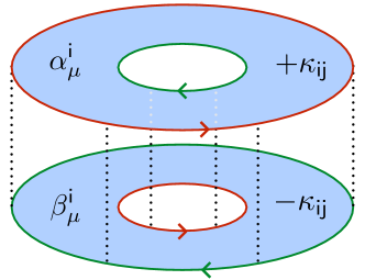
Figure 1: (Color online) Gluing argument for the special case $\Delta=0$. In this case, the CS theory consists of two independent copies, with equal and opposite $K$-matrices. The tunneling processes (dotted lines) that gap out each pair of counterpropagating edge modes couple the two annuli, and the conditions (9) ensure that the two copies of the theory can be consistently “glued” together.

Using these boundary conditions, it is possible to show that Eq. (11) follows in much the same way as its counterpart on the torus, so long as both edges of the annulus are gapped by the same tunneling terms of the form (4). Before proceeding with the full argument, we first provide an intuitive picture of why this is, for the case where $\Delta=0$ in Eq. (1b). In this case, Eq. (6) describes two decoupled CS liquids, one with $K$-matrix $\kappa$ and the other with $K$-matrix $-\kappa$. We can imagine that the two CS liquids live on separate copies of the annulus $A$, which are coupled by the tunneling processes that gap out the edges. The conditions in Eq. (9) ensure that the two coupled annuli can be “glued” together into a single surface, on which lives a composite CS theory with a GSD given by $|\det\kappa|$ (see Fig. 1). Remarkably, these gluing conditions are also sufficient to treat cases where $\Delta\neq 0$, as we now show.

II.3.1 Wilson loops, large gauge transformations, and their algebras

Suppose that we are given a doubled Chern-Simons theory on the annulus of the form (1), and that both edges of the annulus are fully gapped by identical tunneling terms of the form (4). Let us further impose boundary conditions of the form (9) at each edge, with the matrix $T$ chosen appropriately (see the Appendix). We can now use these boundary conditions, arising as they do from the need to cancel the anomalous boundary term (8c), to construct Wilson loop operators, which can in turn be used to determine the dimension of the ground state subspace.

To do this, we first perform a change of basis on the CS Lagrangian (1a) by defining the linear combinations

$$\begin{split}a^{\mathtt{i}}_{+,\mu}&\,\raisebox{0.85pt}{.}\raisebox{2.85pt}{.}\!\!=\,T^{\,}_{\mathtt{ij}}\,\alpha^{\mathtt{j}}_{\mu}+\beta^{\mathtt{i}}_{\mu}\\ a^{\mathtt{i}}_{-,\mu}&\,\raisebox{0.85pt}{.}\raisebox{2.85pt}{.}\!\!=\,\frac{1}{2}\left(\alpha^{\mathtt{i}}_{\mu}-T^{\,}_{\mathtt{ij}}\,\beta^{\mathtt{j}}_{\mu}\right),\end{split}$$ (12a)

where $$\mathtt{i}=1,\dots,N$$. In terms of these fields, the transformed CS Lagrangian reads

$$\mathcal{L}^{\,}_{\mathrm{CS}}= \frac{\epsilon^{\mu\nu\rho}}{4\pi}\,\left(\varkappa^{\,}_{\mathtt{ij}}\,a^{\mathtt{i}}_{+,\mu}\,\partial^{\,}_{\nu}\,a^{\mathtt{j}}_{-,\rho}+\varkappa^{\mathsf{T}}_{\mathtt{ij}}\,a^{\mathtt{i}}_{-,\mu}\,\partial^{\,}_{\nu}\,a^{\mathtt{j}}_{+,\rho}\right.$$

$$\qquad\left.+\widetilde{\varkappa}^{\,}_{\mathtt{ij}}\,a^{\mathtt{i}}_{-,\mu}\,\partial^{\,}_{\nu}\,a^{\mathtt{j}}_{-,\rho}\right),$$ (12b)

where we have defined the $$N\times N$$ matrices

$$\varkappa \,\raisebox{0.85pt}{.}\raisebox{2.85pt}{.}\!\!=\,\kappa\,T-T^{\mathsf{T}}\,\Delta T,$$ (12c)

$$\widetilde{\varkappa} \,\raisebox{0.85pt}{.}\raisebox{2.85pt}{.}\!\!=\,\kappa-\Delta\,T-T^{\mathsf{T}}\,\Delta^{\mathsf{T}}-T^{\mathsf{T}}\,\kappa T.$$ (12d)

Before we continue, note that the linear transformation defined by Eq. (12a) has determinant $$\pm 1 |\det K|$$, so that this change of basis leaves invariant. Consequently, we have that

$$|\det K|=|\det\varkappa|^{2}.$$ (12e)

Furthermore, observe that, in the case $$T=\mathbbm{1} \varkappa T \varkappa$$, the matrix above coincides with the one defined in Eq. (2c). For reasons that will be made clear below, we restrict our attention to cases where the matrix can be chosen such that the matrix has integer entries.

In this new basis, the gluing conditions (9) become Dirichlet boundary conditions on the $(-)$ fields,

$$\chi^{\mathtt{i}}_{-}|^{\,}_{\partial A}=0,\qquad a^{\mathtt{i}}_{-,\mu}|^{\,}_{\partial A}=0,$$ (13)

for $\mathtt{i}=1,\ldots,N$. Rewriting the Lagrangian density in the gauge $a^{\mathtt{i}}_{\pm,0}=0$ (this can be done using a gauge transformation obeying the gluing conditions), we obtain

$$\begin{split}\mathcal{L}^{\,}_{\mathrm{CS}}=&\,\frac{1}{4\pi}\,\left[\varkappa^{\,}_{\mathtt{ij}}\left(a^{\mathtt{i}}_{+,2}\,\partial^{\,}_{0}\,a^{\mathtt{j}}_{-,1}-a^{\mathtt{i}}_{+,1}\,\partial^{\,}_{0}\,a^{\mathtt{j}}_{-,2}\right)\right.\\ &\,\left.+\varkappa^{\mathsf{T}}_{\mathtt{ij}}\,\left(a^{\mathtt{i}}_{-,2}\,\partial^{\,}_{0}\,a^{\mathtt{j}}_{+,1}-a^{\mathtt{i}}_{-,1}\,\partial^{\,}_{0}\,a^{\mathtt{j}}_{+,2}\right)\right.\\ &\,\left.+\widetilde{\varkappa}_{\mathtt{ij}}\,\left(a^{\mathtt{i}}_{-,2}\,\partial^{\,}_{0}\,a^{\mathtt{j}}_{-,1}-a^{\mathtt{i}}_{-,1}\,\partial^{\,}_{0}\,a^{\mathtt{j}}_{-,2}\right)\right]\end{split}$$ (14a)

supplemented by the $$2N a^{\mathtt{i}}_{0} \mathtt{i}=1,\ldots,N$$ constraints arising from the equations of motion for (),

$$\partial^{\,}_{1}\,a^{\mathtt{i}}_{+,2}-\partial^{\,}_{2}\,a^{\mathtt{i}}_{+,1}=0,\qquad\partial^{\,}_{1}\,a^{\mathtt{i}}_{-,2}-\partial^{\,}_{2}\,a^{\mathtt{i}}_{-,1}=0.$$ (14b)

The constraints (14b) are met by the decompositions

$$a^{\mathtt{i}}_{\pm,1}(x^{\,}_{1},x^{\,}_{2},t)=\partial^{\,}_{1}\,\chi^{\mathtt{i}}_{\pm}(x^{\,}_{1},x^{\,}_{2},t)+\bar{a}^{\mathtt{i}}_{\pm,1}(x^{\,}_{1},t),$$ (15a)

$$a^{\mathtt{i}}_{\pm,2}(x^{\,}_{1},x^{\,}_{2},t)=\partial^{\,}_{2}\,\chi^{\mathtt{i}}_{\pm}(x^{\,}_{1},x^{\,}_{2},t)+\bar{a}^{\mathtt{i}}_{\pm,2}(x^{\,}_{2},t),$$ (15b)

of the CS fields, provided that $\chi^{\mathtt{i}}_{\pm}(x^{\,}_{1},x^{\,}_{2},t)$ are everywhere smooth functions of $x^{\,}_{1}$ and $x^{\,}_{2}$, while $\bar{a}^{\mathtt{i}}_{\pm,1}(x^{\,}_{1},t)$ and $\bar{a}^{\mathtt{i}}_{\pm,2}(x^{\,}_{2},t)$ are independent of $x^{\,}_{2}$ and $x^{\,}_{1}$, respectively. Furthermore, the geometry of an annulus is implemented by the boundary conditions

$$\chi^{\mathtt{i}}_{\pm}(x^{\,}_{1},x^{\,}_{2}+2\pi,t)=\chi^{\mathtt{i}}_{\pm}(x^{\,}_{1},x^{\,}_{2},t)$$ (16a)

for the fields parametrizing the pure gauge contributions and

$$\chi^{\mathtt{i}}_{-}(0,x^{\,}_{2},t)=\chi^{\mathtt{i}}_{-}(\pi,x^{\,}_{2},t)=0,$$ (16b)

$$\bar{a}^{\mathtt{i}}_{-,1}(0,t)=\bar{a}^{\mathtt{i}}_{-,1}(\pi,t)=0,$$ (16c)

$$\bar{a}^{\mathtt{i}}_{-,2}(x^{\,}_{2},t)|^{\,}_{x^{\,}_{1}=0}=\bar{a}^{\mathtt{i}}_{-,2}(x^{\,}_{2},t)|^{\,}_{x^{\,}_{1}=\pi}=\bar{a}^{\mathtt{i}}_{-,2}(x^{\,}_{2},t)=0,$$ (16d)

for the gluing conditions. The coordinate system employed in these definitions is depicted in Fig. 2.

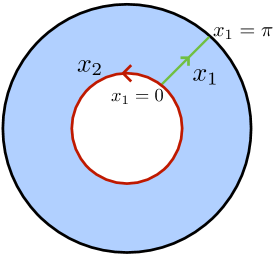
Figure 2: (Color online) Coordinate system on the annulus $A=[0,\pi]\times S^{1}$. The inner boundary is at $x^{\,}_{1}=0$, while the outer boundary is at $x^{\,}_{1}=\pi$. The coordinate $x^{\,}_{2}$ is defined on the circle $S^{1}$.

The next step is to show that the barred variables decouple from the remaining (pure gauge) degrees of freedom. This can be done by inserting the decomposition (15) into the action and using the boundary conditions (16). In the course of this calculation, the terms containing $\widetilde{\varkappa}$ that involve barred variables are found to vanish due to the fact that $\bar{a}^{\mathtt{i}}_{-,2}(x^{\,}_{2},t)=0$ for all $x^{\,}_{2}$ and $t$, and to the periodicity in $x^{\,}_{2}$ of the functions $\chi^{\mathtt{i}}_{-}(x^{\,}_{1},x^{\,}_{2},t)$. We then find an action involving only the matrix $\varkappa$ that governs the barred variables alone,

$$S^{\,}_{\mathrm{top}}=\frac{1}{2\pi}\,\int\limits\mathrm{d}t\ \varkappa^{\,}_{\mathtt{ij}}\,A^{\mathtt{i}}_{2}\,\dot{A}^{\mathtt{j}}_{1},$$ (17a)

where, for all $$\mathtt{i}=1,\ldots,N$$, we have defined the global degrees of freedom

$$A^{\mathtt{i}}_{1}(t)\,\raisebox{0.85pt}{.}\raisebox{2.85pt}{.}\!\!=\,\int\limits\limits_{0}^{\pi}\mathrm{d}x^{\,}_{1}\,\bar{a}^{\mathtt{i}}_{-,1}(x^{\,}_{1},t),$$ (17b)

$$A^{\mathtt{i}}_{2}(t)\,\raisebox{0.85pt}{.}\raisebox{2.85pt}{.}\!\!=\,\int\limits\limits_{0}^{2\pi}\mathrm{d}x^{\,}_{2}\,\bar{a}^{\mathtt{i}}_{+,2}(x^{\,}_{2},t).$$ (17c)

In Eq. (17a), we employ the notation $\dot{A}^{\mathtt{j}}_{1}=\partial^{\,}_{t}A^{\mathtt{j}}_{1}\equiv\partial^{\,}_{0}A^{\mathtt{j}}_{1}$. According to the topological action (17a), the variable $\varkappa^{\,}_{\mathsf{ij}}\,A^{\mathtt{i}}_{2}/(2\pi)$ is canonically conjugate to the variable $A^{\mathtt{j}}_{1}$. Canonical quantization then gives the equal-time commutation relations

$$\left[A^{\mathtt{i}}_{1},A^{\mathtt{j}}_{2}\right] =2\pi\mathrm{i}\,\varkappa^{-1}_{\mathtt{ij}},$$ (18a)

$$\left[A^{\mathtt{i}}_{1},A^{\mathtt{j}}_{1}\right] =\left[A^{\mathtt{i}}_{2},A^{\mathtt{j}}_{2}\right]=0,$$ (18b)

for $\mathtt{i},\mathtt{j}=1,\ldots,N$. We may now define the Wilson loop operators

$$W^{\mathtt{i}}_{1}\,\raisebox{0.85pt}{.}\raisebox{2.85pt}{.}\!\!=\,e^{\mathrm{i}A^{\mathtt{i}}_{1}},\qquad W^{\mathtt{i}}_{2}\,\raisebox{0.85pt}{.}\raisebox{2.85pt}{.}\!\!=\,e^{\mathrm{i}A^{\mathtt{i}}_{2}},$$ (19a)

whose algebra is found to be

$$W^{\mathtt{i}}_{1}\,W^{\mathtt{j}}_{2}=e^{-2\pi\mathrm{i}\,\varkappa^{-1}_{\mathtt{ij}}}\,W^{\mathtt{j}}_{2}\,W^{\mathtt{i}}_{1},$$ (19b)

$$\left[W^{\mathtt{i}}_{1},W^{\mathtt{j}}_{1}\right]=\left[W^{\mathtt{i}}_{2},W^{\mathtt{j}}_{2}\right]=0.$$ (19c)

There is still a set of symmetries that imposes constraints on the dimension of the Hilbert space associated with $S^{\,}_{\mathrm{top}}$. In particular, the path integral is invariant under the “large gauge transformations”

$$A^{\mathtt{i}}_{1,2}\mapsto A^{\mathtt{i}}_{1,2}+2\pi$$ (20)

for any $\mathtt{i}=1,\ldots,N$. The large gauge transformations are implemented by the operators

$$U^{\mathtt{i}}_{1}\,\raisebox{0.85pt}{.}\raisebox{2.85pt}{.}\!\!=\,e^{+\mathrm{i}\,\varkappa^{\,}_{\mathtt{ij}}\,A^{\mathtt{j}}_{2}},\qquad U^{\mathtt{i}}_{2}\,\raisebox{0.85pt}{.}\raisebox{2.85pt}{.}\!\!=\,e^{-\mathrm{i}\,\varkappa^{\,}_{\mathtt{ij}}\,A^{\mathtt{j}}_{1}},$$ (21a)

which satisfy the algebra

$$U^{\mathtt{i}}_{1}\,U^{\mathtt{j}}_{2}=e^{-2\pi\mathrm{i}\,\varkappa^{\,}_{\mathtt{ij}}}\,U^{\mathtt{j}}_{2}\,U^{\mathtt{i}}_{1},$$

$$\left[U^{\mathtt{i}}_{1},U^{\mathtt{j}}_{1}\right]=\left[U^{\mathtt{i}}_{2},U^{\mathtt{j}}_{2}\right]=0,$$ (21b)

for any $\mathtt{i},\mathtt{j}=1,\ldots,N$. Because we require that $\varkappa$ is an integer matrix, this means that

$$\left[U^{\mathtt{i}}_{1},U^{\mathtt{j}}_{2}\right]=\left[U^{\mathtt{i}}_{1},U^{\mathtt{j}}_{1}\right]=\left[U^{\mathtt{i}}_{2},U^{\mathtt{j}}_{2}\right]=0$$ (22)

for all $\mathtt{i},\mathtt{j}=1,\ldots,N$. Hence, all $U^{\mathtt{i}}_{1}$, $U^{\mathtt{i}}_{2}$ with $\mathtt{i}=1,\ldots,N$ can be diagonalized simultaneously. Since any one of $U^{\mathtt{i}}_{1}$ and $U^{\mathtt{i}}_{2}$ generates a transformation that leaves the path integral invariant, the vacua of the theory must be eigenstates of any one of $U^{\mathtt{i}}_{1}$ and $U^{\mathtt{i}}_{2}$ for ${\mathtt{i}}=1,\ldots,N$.

II.3.2 Dimension of the ground-state subspace

In order to determine the GSD of the theory, it suffices to determine the number of eigenstates of any one of $U^{\mathtt{i}}_{1}$ and $U^{\mathtt{i}}_{2}$ for ${\mathtt{i}}=1,\ldots,N$. To do this, we follow the argument of Wesolowski et al., Wesolowski et al. (1994) which can be adapted to our case with only minor modifications.

First, we define the eigenstates of any one of $U^{\mathtt{i}}_{1}$ and $U^{\mathtt{i}}_{2}$ for ${\mathtt{i}}=1,\ldots,N$ by

$$U^{\mathtt{i}}_{1}\,\ket{\Psi}=e^{\mathrm{i}\gamma^{\mathtt{i}}_{1}}\,\ket{\Psi},\qquad U^{\mathtt{i}}_{2}\,\ket{\Psi}=e^{\mathrm{i}\gamma^{\mathtt{i}}_{2}}\,\ket{\Psi}.$$ (23)

Since $A^{\mathtt{i}}_{1}$ and $A^{\mathtt{j}}_{2}$ do not commute, we may choose to represent the state $\ket{\Psi}$ in the basis for which $A^{\mathtt{i}}_{1}$ is diagonal by

$$\psi(\{A^{\mathtt{i}}_{1}\})\,\raisebox{0.85pt}{.}\raisebox{2.85pt}{.}\!\!=\,\braket{\{A^{\mathtt{i}}_{1}\}}{\Psi}.$$ (24)

The representation $\psi(\{A^{\mathtt{i}}_{2}\})$ follows from the representation $\psi(\{A^{\mathtt{i}}_{1}\})$ by a change of basis to the one in which $A^{\mathtt{i}}_{2}$ is diagonal. The large gauge transformations (21a) are represented by

$$U^{\mathtt{i}}_{1}\,\raisebox{0.85pt}{.}\raisebox{2.85pt}{.}\!\!=\,e^{2\pi\,\partial/\partial A^{\mathtt{i}}_{1}},\qquad U^{\mathtt{i}}_{2}\,\raisebox{0.85pt}{.}\raisebox{2.85pt}{.}\!\!=\,e^{-\mathrm{i}\,\varkappa^{\,}_{\mathtt{ij}}\,A^{\mathtt{j}}_{1}},$$ (25)

in the basis (24). The eigenvalue problem then becomes

$$U^{\mathtt{i}}_{1}\,\psi(\{A^{\mathtt{i}}_{1}\})\,\raisebox{0.85pt}{.}\raisebox{2.85pt}{.}\!\!=\, \,\psi\left(A^{1}_{1},\ldots,A^{\mathtt{i}}_{1}+2\pi,\ldots,A^{N}_{1}\right)$$

$$\equiv \,e^{\mathrm{i}\gamma^{\mathtt{i}}_{1}}\,\psi(\{A^{\mathtt{i}}_{1}\}),$$ (26a)

$$U^{\mathtt{i}}_{2}\,\psi(\{A^{\mathtt{i}}_{1}\})\,\raisebox{0.85pt}{.}\raisebox{2.85pt}{.}\!\!=\, \,e^{-\mathrm{i}\,\varkappa^{\,}_{\mathtt{ij}}\,A^{\mathtt{j}}_{1}\,\psi(\{A^{\mathtt{i}}_{1}\})}$$

$$\equiv \,e^{\mathrm{i}\gamma^{\mathtt{i}}_{2}}\,\psi(\{A^{\mathtt{i}}_{1}\}).$$ (26b)

Equation (26a) implies that we can write the following series for $\psi$,

$$\psi(\{A^{\mathtt{i}}_{1}\})\equiv\psi(\bm{A}^{\,}_{1})=e^{\mathrm{i}\bm{\gamma}^{\,}_{1}\cdot\bm{A}^{\,}_{1}/2\pi}\,\sum_{\bm{n}}d(\bm{n})\,e^{\mathrm{i}\bm{n}\cdot\bm{A}^{\,}_{1}},$$ (27)

where $\bm{n}=(n^{\,}_{1},\ldots,n^{\,}_{N})^{\mathsf{T}}\in\mathbb{Z}^{N}$, $\bm{A}^{\,}_{1}=(A^{1}_{1},\ldots,A^{N}_{1})^{\mathsf{T}}\in\mathbb{R}^{N}$, and $\bm{\gamma}^{\,}_{1}=(\gamma^{1}_{1},\ldots,\gamma^{N}_{1})^{\mathsf{T}}\in\mathbb{R}^{N}$.

Second, we seek the constraints on the real-valued coefficients $d(\bm{n})$ entering the expansion (27) that, as we shall demonstrate, fix the dimension of the ground-state subspace. To this end, we extract from the $N\times N$ matrix $\varkappa$ that was defined in Eq. (2c) the family

$$\varkappa\,=\!\!\raisebox{0.85pt}{.}\raisebox{2.85pt}{.}\,\begin{pmatrix}\bm{k}^{\,\mathsf{T}}_{1}\\ \vdots\\ \bm{k}^{\,\mathsf{T}}_{N}\end{pmatrix}$$ (28a)

of $$N \mathbb{Z}^{N} \varkappa^{-1}$$ vectors from and from its inverse the family

$$\varkappa^{-1}\,=\!\!\raisebox{0.85pt}{.}\raisebox{2.85pt}{.}\,\begin{pmatrix}\bm{\ell}^{\,}_{1}&\ldots&\bm{\ell}^{\,}_{N}\end{pmatrix}$$ (28b)

of $$N \mathbb{Q}^{N}$$ vectors from . By construction, these vectors satisfy

$$\bm{k}^{\,}_{\mathtt{i}}\cdot\bm{\ell}^{\,}_{\mathtt{j}}=\delta^{\,}_{\mathtt{ij}}.$$ (28c)

Using these vectors, we observe that inserting the series (27) into the left-hand side of Eq. (26b) gives

$$U^{\mathtt{i}}_{2}\,\psi(\bm{A}^{\,}_{1})= \,e^{\mathrm{i}\bm{\gamma}^{\,}_{1}\cdot\bm{A}^{\,}_{1}/(2\pi)}\,e^{-\mathrm{i}\bm{k}^{\,}_{\mathtt{i}}\cdot\bm{A}^{\,}_{1}}\,\sum_{\bm{n}}d(\bm{n})\,e^{\mathrm{i}\bm{n}\cdot\bm{A}^{\,}_{1}}$$

$$= \,e^{\mathrm{i}\bm{\gamma}^{\,}_{1}\cdot\bm{A}^{\,}_{1}/(2\pi)}\,\sum_{\bm{n}}d(\bm{n}+\bm{k}^{\,}_{\mathtt{i}})\,e^{\mathrm{i}\bm{n}\cdot\bm{A}^{\,}_{1}}$$

$$= \,e^{\mathrm{i}\gamma_{2}^{\mathtt{i}}}\,\psi(\bm{A}^{\,}_{1}),$$ (29)

which implies

$$d(\bm{n}+\bm{k}^{\,}_{\mathtt{i}})=e^{\mathrm{i}\gamma^{\mathtt{i}}_{2}}\,d(\bm{n})$$ (30)

for all ${\mathtt{i}}=1,\ldots,N$. The constraint (30) is automatically satisfied by demanding that

$$d(\bm{n})=e^{\mathrm{i}\bm{\gamma}^{\,}_{2}\cdot(\varkappa^{-1})^{\mathsf{T}}\bm{n}}\,\tilde{d}(\bm{n})$$ (31a)

with

$$\tilde{d}(\bm{n})=\tilde{d}(\bm{n}+\bm{k}^{\,}_{\mathtt{i}}),$$ (31b)

since

$$\bm{\gamma}^{\,}_{2}\cdot(\varkappa^{-1})^{\mathsf{T}}\,\bm{k}^{\,}_{\mathtt{i}}=\gamma^{\mathtt{j}}_{2}(\bm{\ell}^{\,}_{\mathtt{j}}\cdot\bm{k}^{\,}_{\mathtt{i}})=\gamma^{\mathtt{i}}_{2}.$$ (31c)

Hence, insertion of (31a) into the expansion (27) that solves the eigenvalue problem (26a) gives the expansion

$$\psi(\bm{A}^{\,}_{1})=e^{\mathrm{i}\bm{\gamma}^{\,}_{1}\cdot\bm{A}^{\,}_{1}/(2\pi)}\sum_{\bm{n}}e^{\mathrm{i}\bm{\gamma}^{\,}_{2}\cdot(\varkappa^{-1})^{\mathsf{T}}\bm{n}}\,\tilde{d}(\bm{n})\,e^{\mathrm{i}\bm{n}\cdot\bm{A}^{\,}_{1}}$$ (32)

that solves the eigenvalue problem (26b).

Third, condition (31b) implies that the set of vectors $\{\bm{n}\}$ forms a lattice with basis vectors $\{\bm{k}^{\,}_{\mathtt{i}}\}$. The number of inequivalent points in the lattice is therefore given by

$$r\,\raisebox{0.85pt}{.}\raisebox{2.85pt}{.}\!\!=\,\left|\det\begin{pmatrix}\bm{k}^{\,}_{1}&\ldots&\bm{k}^{\,}_{N}\end{pmatrix}\right|=\left|\det\,\varkappa^{\mathsf{T}}\right|=|\det\,\varkappa|.$$ (33)

This means that we can decompose any $\bm{n}$ as

$$\bm{n}=\bm{v}^{\,}_{m}+p^{\,}_{\mathtt{i}}\,\bm{k}^{\,}_{\mathtt{i}},$$ (34)

where $p^{\,}_{\mathtt{i}}\in\mathbb{Z}$ and we have introduced $r$ linearly independent vectors $\bm{v}^{\,}_{m}$. We can therefore rewrite

$$\psi(\bm{A}^{\,}_{1})=\sum_{m=1}^{r}\tilde{d}^{\,}_{m}\,f^{\,}_{m}(\bm{A}^{\,}_{1}),$$ (35a)

where

$$\tilde{d}^{\,}_{m}\,\raisebox{0.85pt}{.}\raisebox{2.85pt}{.}\!\!=\,\tilde{d}(\bm{v}^{\,}_{m}+p^{\,}_{\mathtt{i}}\,\bm{k}^{\,}_{\mathtt{i}})=\tilde{d}(\bm{v}^{\,}_{m}),$$ (35b)

and

$$\begin{split}f^{\,}_{m}(\bm{A}^{\,}_{1})\,\raisebox{0.85pt}{.}\raisebox{2.85pt}{.}\!\!=\,&\,e^{\mathrm{i}\bm{\gamma}^{\,}_{1}\cdot\bm{A}^{\,}_{1}/(2\pi)}\\ &\,\times\!\!\!\!\sum_{p^{\,}_{1},\ldots,p^{\,}_{N}}\!\!\!\!e^{\mathrm{i}\bm{\gamma}^{\,}_{2}\cdot(\varkappa^{-1})^{\mathsf{T}}\left(\bm{v}^{\,}_{m}+p^{\,}_{\mathtt{i}}\,\bm{k}^{\,}_{\mathtt{i}},\right)}\,e^{\mathrm{i}(\bm{v}^{\,}_{m}+p^{\,}_{\mathtt{i}}\,\bm{k}^{\,}_{\mathtt{i}})\cdot\bm{A}^{\,}_{1}}.\end{split}$$ (35c)

Since any $\psi(\bm{A}^{\,}_{1})$ in the ground-state manifold can be written in this way, we have demonstrated that there are $r=|\det\,\varkappa|$ linearly independent ground-state wavefunctions $f^{\,}_{m}(\bm{A}^{\,}_{1})$ in the topological Hilbert space. In other words, we have shown that

$$\begin{split}\text{GSD}&=|\det\,\varkappa|=\sqrt{|\det K|},\end{split}$$ (36)

with $K$ defined in Eq. (1b). This is precisely the result advertised in Eq. (11). Note that because $\varkappa$ is an integer-valued matrix, it has an integer-valued determinant. Consequently, $\sqrt{|\det K|}=|\det\varkappa|$ is an integer.

II.3.3 Generalization to manifolds with multiple holes

It is instructive to consider generalizing these arguments to the case of a system with the topology of an $N^{\,}_{\mathrm{h}}$-punctured disk. In this generalization, the boundary can be viewed as the disjoint union of $N^{\,}_{\mathrm{h}}+1$ copies of $S^{1}$. Since each of these edges is gapped, anomaly cancellation enforces independent gluing conditions for each copy of $S^{1}$. In principle, a different matrix $T$ could be chosen for each boundary. This could happen if, for example, different edges are gapped by different sets of tunneling vectors $\bm{T}$ that enter Eq. (4). If this is the case, then it may not be possible to find a linear transformation of the form (12a) such that $N$ of the CS fields obey Dirichlet boundary conditions on all edges, as in Eq. (13). The remainder of the argument presented here for counting the degeneracy then breaks down. Finding an alternative argument that applies in these cases is an interesting problem for future work, but is beyond the scope of this paper.

In the case where all boundaries are gapped in the same way, however, one obtains a set of Wilson loops like those in Eqs. (19a) for each hole. [See, e.g., Eqs. (37) in the next section.] Since these sets of Wilson loops are completely independent, one obtains a degeneracy of size $|\det\,K|^{N^{\,}_{\mathrm{h}}/2}$.

III Applications

(a)
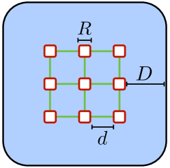
(b)

Figure 3: (Color online) A punctured TRS-FTL with gapped edges. (a) Schematic representation of an “artificial” spin-like system. In the limit $D\gg d,R$, each hole (white square) carries with it a $q$-fold topological degeneracy that is split exponentially by tunneling processes that encircle (red lines) or connect (green lines) the holes. (b) Wilson loops defined in Eqs. (37). The dashed line represents the product of the two Wilson loops above it, which connects the two holes.

With the results of Sec. II in hand, we now explore some of the consequences of Eq. (11). We begin by examining the fate of the topological degeneracy in finite-sized systems, before considering the possibility of using calorimetry to detect experimental signatures of the degeneracy. We close the section by re-evaluating the proposed Hansson et al. (2004) topological field theory for the $s$-wave BCS superconductor in light of the results of this paper.

III.1 Finite systems: clock models and beyond

On closed manifolds, the topological degeneracy is exact only in the limit of infinite system size. This is a result of the fact, pointed out by Wen and Niu, Wen and Niu (1990) that quasiparticle tunneling events over distances of the order of the system size lift the topological degeneracy by a splitting that is exponentially small in the linear size of the system. This observation was also confirmed numerically for the case of the (2+1)-dimensional Abelian Higgs model on the torus by Vestergren et al. in Refs. Vestergren et al., 2005 and Vestergren and Lidmar, 2005. A similar splitting occurs for manifolds with boundary, like those studied in this work. For a planar system with many holes, each of which carries a $q$-fold degeneracy (where $q\,\raisebox{0.85pt}{.}\raisebox{2.85pt}{.}\!\!=\,\sqrt{|\det\,K|}$) in the limit of infinite system size, there are two kinds of tunneling events that can lift the degeneracy. These are (1) tunnelings that encircle a single hole and (2) tunnelings between boundaries. Below we argue that, in a finite-sized system with $N^{\,}_{\mathrm{h}}$ holes, the array of $N^{\,}_{\mathrm{h}}$ coupled $q$-state degrees of freedom can be modeled as a spin-like system [see Fig. 3(a)].

To see how this arises, we first note that for a system with $N^{\,}_{\mathrm{h}}$ holes it is possible to define a set of Wilson loops for each hole. Analogously to Eqs. (19a), for any $\mathtt{i}=1,\ldots,N$ we define

$$W^{\mathtt{i}}_{1,j}\,\raisebox{0.85pt}{.}\raisebox{2.85pt}{.}\!\!=\,\exp\Bigg{(}\mathrm{i}\int\limits_{\mathcal{C}^{\,}_{1,j}}\mathrm{d}\bm{\ell}\cdot\bar{\bm{a}}^{\mathtt{i}}_{-}(\bm{x},t)\Bigg{)},$$ (37a)

$$W^{\mathtt{i}}_{2,j}\,\raisebox{0.85pt}{.}\raisebox{2.85pt}{.}\!\!=\,\exp\Bigg{(}\mathrm{i}\oint\limits_{\mathcal{C}^{\,}_{2,j}}\mathrm{d}\bm{\ell}\cdot\bar{\bm{a}}^{\mathtt{i}}_{+}(\bm{x},t)\Bigg{)},$$ (37b)

where the open curve $$\mathcal{C}^{\,}_{1,j} j \mathcal{C}^{\,}_{2,j} j j k$$ connects the -th hole to the outer boundary, and the closed curve encircles the -th hole [see Fig. (3)(b)]. Each set of operators obeys an independent copy of the algebra (19c). Furthermore, for any pair of holes and , the Wilson loop

$$W^{\mathtt{i}}_{1,jk}\,\raisebox{0.85pt}{.}\raisebox{2.85pt}{.}\!\!=\,W^{\mathtt{i}\,{\dagger}}_{1,j}\,W^{\mathtt{i}}_{1,k}$$ (37c)

connects these holes. More generally, any number of holes can be connected by compositions of the Wilson loops defined in Eqs. (37). In an infinite system, the topological protection of the degeneracy (36) arises because the Wilson loops defined in Eqs. (19a) are nonlocal operators and are therefore forbidden from entering the Hamiltonian. In a finite system, however, the Wilson loops are no longer nonlocal degrees of freedom and can therefore enter the effective theory. In principle, all powers and combinations of the Wilson loops are allowed to enter the effective Hamiltonian

$$H^{\,}_{\mathrm{eff}}\,\raisebox{0.85pt}{.}\raisebox{2.85pt}{.}\!\!=\, \,\sum_{{\mathtt{i}}=1}^{N}\sum_{j=1}^{N^{\,}_{\mathrm{h}}}\Bigg{(}h^{\mathtt{i}}_{1,j}\,W^{\mathtt{i}}_{1,j}+h^{\mathtt{i}}_{2,j}\,W^{\mathtt{i}}_{2,j}+\sum_{k=1}^{N^{\,}_{\mathrm{h}}}J^{\mathtt{i}}_{jk}\,W^{\mathtt{i}}_{1,jk}$$

$$\,+\ldots\Bigg{)},$$ (38)

where the omitted terms include higher powers of the Wilson loops as well as all necessary Hermitian conjugates. In practice, however, all couplings in $H^{\,}_{\mathrm{eff}}$ are exponentially small in the shortest available length scale, which limits the tunneling rates. For example, $J^{\mathtt{i}}_{jk}\propto e^{-c\,d_{jk}/\xi}$, where $c$ is a constant of order one, $d_{jk}$ is the distance between holes $j$ and $k$ [see Fig. 3(a)], and $\xi$ is a length scale associated with quasiparticle tunneling. foo (a)

It is interesting to note that the Hamiltonian $H^{\,}_{\mathrm{eff}}$ admits a certain amount of external control – the holes can be arranged in arbitrary ways, and the magnitudes of the couplings can be tuned by changing the length scales $R$, $d^{\,}_{jk}$, and $D$ defined in Fig. 3. In particular, many terms in $H^{\,}_{\mathrm{eff}}$ can be tuned to zero by varying these length scales. We will make use of this freedom below.

To illustrate in what sense the effective Hamiltonian (III.1) can be thought of as a spin-like system, we consider a specific class of examples. In particular, we consider the family of TRS-FTLs defined by

$$K\,\raisebox{0.85pt}{.}\raisebox{2.85pt}{.}\!\!=\,\begin{pmatrix}q&0\\ 0&-q\end{pmatrix},\qquad\bm{Q}\,\raisebox{0.85pt}{.}\raisebox{2.85pt}{.}\!\!=\,\begin{pmatrix}2\\ 2\end{pmatrix},$$ (39)

where $q$ is an even integer. One verifies using Eq. (5) that a single tunneling term of the form (4) with $\bm{T}=(1,-1)^{\mathsf{T}}$ is sufficient to gap out the counterpropagating edge modes without breaking TRS as defined in Ref. Neupert et al., 2011. (The gluing conditions (9) can be implemented by the $1\times 1$ gluing “matrix” $T=1$.) In this case, Eq. (11) predicts a $q$-fold degeneracy per hole. To obtain the explicit effective Hamiltonian, we define

$$\sigma^{\,}_{j}\,\raisebox{0.85pt}{.}\raisebox{2.85pt}{.}\!\!=\,W^{\,}_{1,j},\qquad\tau^{\,}_{j}\,\raisebox{0.85pt}{.}\raisebox{2.85pt}{.}\!\!=\,W^{\,}_{2,j},$$ (40a)

whose only nonvanishing commutation relations arise from the algebra [recall Eq. (19b)]

$$\sigma^{\,}_{j}\,\tau^{\,}_{j}=e^{-2\pi\mathrm{i}/q}\,\tau^{\,}_{j}\,\sigma^{\,}_{j}.$$ (40b)

One can check by writing down explicit representations of $\sigma^{\,}_{j}$ and $\tau^{\,}_{j}$ that they also satisfy

$$\sigma^{q}_{j}=\tau^{q}_{j}=\mathbbm{1}.$$ (41)

For example, in the case $q=2$ we may use Pauli matrices, e.g.,

$$\sigma^{\,}_{j}=\sigma^{\,}_{z},\qquad\tau^{\,}_{j}=\sigma^{\,}_{x},$$ (42)

and in the case $q=4$ we may use

$$\sigma^{\,}_{j}\,\raisebox{0.85pt}{.}\raisebox{2.85pt}{.}\!\!=\,\text{diag}\left(1,\,e^{-\mathrm{i}\,\pi/2},\,e^{-\mathrm{i}\,\pi},\,e^{-\mathrm{i}\,3\pi/2}\right),$$ (43a)

$$\tau^{\,}_{j}\,\raisebox{0.85pt}{.}\raisebox{2.85pt}{.}\!\!=\,\begin{pmatrix}0&0&0&1\\ 1&0&0&0\\ 0&1&0&0\\ 0&0&1&0\end{pmatrix}.$$ (43b)

For a system with $N^{\,}_{\mathrm{h}}$ holes of size $R$ arranged in a one-dimensional chain with lattice spacing $d$, the effective Hamiltonian in the limit $D\gg d,R$ (with $D,d,R$ defined in Fig. 3) becomes that of a one-dimensional $\mathbb{Z}^{\,}_{q}$ quantum clock model (see Ref. fen, and references therein),

$$H^{\,}_{\mathrm{eff}}\,\raisebox{0.85pt}{.}\raisebox{2.85pt}{.}\!\!=\,\sum_{i=1}^{N^{\,}_{\mathrm{h}}-1}J^{\,}_{i}\,\left(\sigma^{{\dagger}}_{i}\,\sigma^{\,}_{i+1}+\text{H.c.}\right)+\sum_{i=1}^{N^{\,}_{\mathrm{h}}}h^{\,}_{i}\left(\tau^{\,}_{i}+\text{H.c.}\right),$$ (44)

where $J^{\,}_{i}\propto e^{-c^{\,}_{1}\,d/\xi}$ and $h^{\,}_{i}\propto e^{-c^{\,}_{2}\,R/\xi}$, with the real constants $c^{\,}_{1}$ and $c^{\,}_{2}$ of order unity. For simplicity, we have constrained the couplings $J^{\,}_{i}$ and $h^{\,}_{i}$ to be real, although their magnitude and sign is allowed to vary from hole to hole (hence the subscripts $i$). Note that in the above Hamiltonian, terms linear in $\sigma^{\,}_{j}$ do not appear, as the associated couplings are suppressed by factors of order $e^{-c^{\,}_{3}\,D/\xi}\ll e^{-c^{\,}_{1}\,d/\xi},\ e^{-c^{\,}_{2}\,R/\xi}$. Similarly, longer-range two-body terms, as well as higher powers of the $\sigma^{\,}_{j}$ and $\tau^{\,}_{j}$, are also omitted, as they correspond to higher-order tunneling processes.

The Hamiltonian of the clock model (44) is invariant under the symmetry operation

$$H^{\,}_{\mathrm{eff}}\mapsto\mathcal{S}\,H^{\,}_{\mathrm{eff}}\,\mathcal{S}^{-1}$$ (45a)

generated by

$$\mathcal{S}\,\raisebox{0.85pt}{.}\raisebox{2.85pt}{.}\!\!=\,\prod_{i=1}^{N^{\,}_{\mathrm{h}}}\tau^{{\dagger}}_{i}.$$ (45b)

Indeed, under conjugation by $\mathcal{S}$, $\tau^{{\dagger}}_{j}\mapsto\tau^{{\dagger}}_{j}$ and $\sigma^{{\dagger}}_{j}\mapsto e^{-2\pi\mathrm{i}/q}\sigma^{{\dagger}}_{j}$ for all $j$. This $\mathbbm{Z}^{\,}_{q}$ symmetry can be thought of as a remnant of the $q^{N^{\,}_{\mathrm{h}}}$-fold topological degeneracy of the TRS-FTL, which would be present in the limit $d,R,D\to\infty$.

Before closing this section, we point out that quantum clock models like the one discussed in this section have arisen in various contexts elsewhere in the recent literature, especially in quantum Hall systems with defects. Barkeshli et al. (2014); Clarke et al. (2013); Vaezi (2014); Mong et al. (2014)

III.2 Probing the topological degeneracy with calorimetry

In this section, we consider experimental avenues to detect the topological degeneracy of a punctured TRS-FTL. We focus our attention on calorimetry as a possible probe. In a sample with $N^{\,}_{\mathrm{h}}$ holes, the ground state degeneracy provides a contribution $S^{\,}_{\mathrm{GSD}}=N^{\,}_{\mathrm{h}}\,k^{\,}_{\mathrm{B}}\ln q$, where $k^{\,}_{\mathrm{B}}$ is the Boltzmann constant and $q=\sqrt{\det K}$, to the total entropy $S^{\,}_{\mathrm{tot}}$. If the areal density of holes is kept fixed, then for a sample of length $L$, we have $S^{\,}_{\mathrm{GSD}}\sim L^{2}$ for the topological contribution, which is extensive. This suggests that, were a suitable material to be discovered, one might be able to detect the topological degeneracy of a punctured TRS-FTL by measuring its heat capacity. Such a measurement is feasible with current technology, as membrane-based nanocalorimeters enable the determination of heat capacities $C^{\,}_{V}$ in microgram samples (and smaller), to an accuracy of $\delta C^{\,}_{V}/C^{\,}_{V}\sim 10^{-4}$–$10^{-5}$ down to temperatures of order $100$ mK. Garden et al. (2009); Ong et al. (2006); Tagliati et al. (2012); Tagliati and Rydh (2012)

We first determine the topological contribution to the heat capacity for some particular examples. To do this, we return to the class of TRS-FTLs defined in Eq. (39). The heat capacity in this case is easiest to determine from the clock model of Eq. (44) in the paramagnetic limit $J^{\,}_{i}\to 0$, which is achieved for $d\gg R$ [see Fig. 3(a)]. Setting $h^{\,}_{i}=h$ for convenience, we see that the clock model can be rewritten, after a change of basis, as

$$H^{\,}_{\mathrm{eff}}=h\sum_{i=1}^{N^{\,}_{\mathrm{h}}}\left(\sigma^{\,}_{i}+\sigma^{{\dagger}}_{i}\right)=2h\sum_{i=1}^{N^{\,}_{\mathrm{h}}}\cos\left(\frac{2\pi}{q}\,n^{\,}_{i}\right),$$ (46)

where $n^{\,}_{i}=0,\ldots,q-1$. Consequently the partition function is given by

$$Z=\left(\sum_{n=0}^{q-1}e^{-2\beta\,h\,\cos(2\pi\,n/q)}\right)^{N^{\,}_{\mathrm{h}}},$$ (47)

where $\beta\,\raisebox{0.85pt}{.}\raisebox{2.85pt}{.}\!\!=\,1/(k^{\,}_{\mathrm{B}}\,T)$ and $T$ is the temperature. The topological heat capacity at constant volume, $C^{\mathrm{top}}_{V}$, is then determined from the partition function by standard methods. For example,

$$C^{\mathrm{top}}_{V}=N^{\,}_{\mathrm{h}}\,\frac{h^{2}}{k^{\,}_{\mathrm{B}}\,T^{2}}\times\begin{cases}4\,\text{sech}^{2}\left(\frac{2\,h}{k^{\,}_{\mathrm{B}}\,T}\right),&q=2,\\ 2\,\text{sech}^{2}\left(\frac{h}{k^{\,}_{\mathrm{B}}\,T}\right),&q=4,\\ \frac{9\,\cosh\left(\frac{h}{k^{\,}_{\mathrm{B}}\,T}\right)+\cosh\left(\frac{3\,h}{k^{\,}_{\mathrm{B}}\,T}\right)+8}{\left[2\,\cosh\left(\frac{h}{k^{\,}_{\mathrm{B}}\,T}\right)+\cosh\left(\frac{2\,h}{k^{\,}_{\mathrm{B}}\,T}\right)\right]^{2}},&q=6,\end{cases}$$ (48)

and so on.

To date, there has been no experimental realization of a TRS-FTL or fractional topological insulator. Since background contributions to the heat capacity are material-dependent, it is difficult to provide a precise estimate of the observable effect. However, we can nevertheless identify some constraints on the possible materials that would favor such a measurement.

To do this, let us estimate the various background contributions to the heat capacity of a TRS-FTL. First, we note that, because any TRS-FTL must have a gap $\Delta$, the electronic contribution $C^{\mathrm{el}}_{V}$ to the heat capacity is

$$C^{\mathrm{el}}_{V}\propto\frac{\Delta}{T}\,e^{-\eta\,\Delta/(k^{\,}_{\mathrm{B}}\,T)},$$ (49a)

where $$\eta C^{\mathrm{el}}_{V}$$ is a constant of order one. The exponential suppression of implies that this contribution is always negligible at sufficiently small temperatures.

However, one must also consider the phononic contribution, which follows a Debye power law at low temperatures. This contribution scales with the sample volume, which could be three-dimensional if the TRS-FTL is formed in a heterostructure, as is the case in quantum Hall systems. This fact, which was noted in Ref. Cooper and Stern, 2009, poses the greatest challenge to detecting the topological contribution to the heat capacity, which scales with the area of the two-dimensional sample. In principle, however, one may assume that the TRS-FTL lives in a strictly two-dimensional sample, or at least in a thin film. In this case, we have that the phononic contribution $C^{\mathrm{ph}}_{V}$ to the heat capacity is

$$C^{\mathrm{ph}}_{V}\propto k^{\,}_{\mathrm{B}}\,(T/T^{\,}_{\mathrm{D}})^{2},$$ (49b)

where $T^{\,}_{\mathrm{D}}$ is the Debye temperature (100 K, say). foo (b) We verified numerically, by simulating a square lattice of masses and springs, that the presence or absence of holes has little effect on the phonon spectrum as long as the holes are sufficiently small. We therefore expect the Debye law to hold both with and without holes, as long as one takes into account the excluded volume due to the holes.

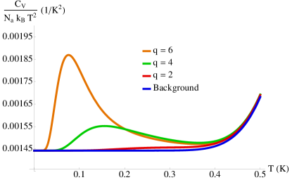
Figure 4: (Color online) Total heat capacity for a monolayer TRS-FTL with $N^{\,}_{\mathrm{a}}=10^{14}$. The topological contribution is shown (above background) for $q=2,4,$ and $6$. The parameters used for the topological contribution were $\nu=5\times 10^{-6}$ ($\sim 22000^{2}$ holes) and $h/k^{\,}_{\mathrm{B}}\approx 0.321$ K, which leads to a maximum excess (for $q=6$) of $\sim 30\%$ over the background (blue curve) near $T=0.1$ K.

The total heat capacity is obtained by adding the three contributions:

$$C^{\,}_{V}(T)=N^{\,}_{\mathrm{a}}\,\left[C^{\mathrm{top}}_{V}(T)+\nu\,C^{\mathrm{ph}}_{V}(T)+\frac{1}{N^{\,}_{\mathrm{a}}}\,C^{\mathrm{el}}_{V}(T)\right],$$ (49c)

where $N^{\,}_{\mathrm{a}}$ is the number of atoms in the sample and $\nu\,\raisebox{0.85pt}{.}\raisebox{2.85pt}{.}\!\!=\,N^{\,}_{\mathrm{h}}/N^{\,}_{\mathrm{a}}$ determines the number of holes. The above formula leads to the estimate of the specific heat curve presented in Fig. 4. A square array of $22000$ holes on a side produces an excess of up to $30\%$ (for $q=6$) on top of the background at $T=0.1$ K, which is well above the experimental error $\delta C^{\,}_{V}/C^{\,}_{V}\sim 10^{-4}$.

We now comment on possible difficulties with this measurement. Perhaps the most important of these is the fact that the energy scales $J^{\,}_{i}$ and $h^{\,}_{i}$ entering Eq. (44) are unknown. It may be possible to circumvent this issue by exploiting the exponential sensitivity of the couplings to the length scales $R$ and $d$. For example, one could prepare samples with $d\gg R$ to eliminate the first term in Eq. (44), and compare results for different values of $R$ to determine whether it is possible to resolve the effect. As long as $h\gtrsim 0.1\,\Delta$, it should be possible to tune $R$ such that the effect is visible.

The presence of disorder in the sample is another potential source of difficulty, as localized states due to disorder can also contribute to the entropy. However, intuition from noninteracting systems, where these states provide a logarithmic correction to the entropy,foo (c) suggests that this contribution would be subleading as compared to the power-law contribution $S_{\rm GSD}\sim L^{2}$ that we predict for a fixed areal density of holes.

III.3 Are superconductors topologically ordered?

In an insightful paper, it was argued by Hansson et al. in Ref. Hansson et al., 2004 that ordinary $s$-wave BCS superconductors are topologically ordered. In fact, it was shown that, when the electromagnetic gauge field is treated dynamically and confined to (2+1) dimensional space and time, the superconductor admits a description in terms of a BF theory like the one defined in Eqs. (2), with

$$\tilde{K}=\begin{pmatrix}0&2\\ 2&0\end{pmatrix}.$$ (50)

Furthermore, it was shown that the edge states that arise when the above theory is defined in a finite planar geometry are generically gapped by Cooper pair creation terms. The proposed theory is consistent with the time-reversal symmetry of the $s$-wave superconductor and captures the statistical phase of $\pi$ that is acquired by an electron upon encircling a vortex. This effective theory, which is the same as that of the $\mathbbm{Z}^{\,}_{2}$ lattice gauge theory in its deconfined phase, predicts a four-fold GSD on the torus, whose exponential splitting in finite systems was verified numerically in Refs. Vestergren et al., 2005 and Vestergren and Lidmar, 2005.

Since the theory defined by Eq. (50) falls squarely within the class of theories studied in this paper, it is tempting to draw the conclusion that the $s$-wave superconductor exhibits a two-fold GSD on the annulus. Below we argue that, while this is indeed the case, the degeneracy is not exponential but power-law in nature, and therefore is not what one might call a topological degeneracy in the canonical sense of Refs. Wen, 1989–Wen, 1991. The reason for this is that the topological nature of the superconductor results from the dynamics of the electromagnetic gauge field, which, in a real planar superconductor, is not confined to the sample itself, but rather extends through all three spatial dimensions. Consequently, the true electromagnetic gauge field that is present in the superconductor can be measured by local external probes.

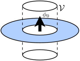
Figure 5: (Color online) Trapping a flux quantum inside a superconducting ring. Confining the flux inside the ring costs no energy for the electrons inside the superconductor, but there is an electromagnetic energy cost obtained by integrating the enclosed magnetic field intensity over the interior of the dashed cylinder, which we denote $\mathcal{V}$.

To see how this coupling to the environment lifts the degeneracy in a power-law fashion, let us consider the origin of the two-fold degeneracy. Recall that for an annular superconductor (a thin-film mesoscopic ring, for example), the phase of the superconducting order parameter winds by $2\pi$ around the hole if a flux quantum $\phi^{\,}_{0}=h/2e$ is trapped inside. This indicates that the electronic spectrum of the superconductor cannot be used to distinguish between cases where an even ($\phi=0$ mod $\phi^{\,}_{0}$) or odd ($\phi=1$ mod $\phi^{\,}_{0}$) number of flux quanta penetrate the hole. This is precisely the origin of the degeneracy. However, because the electromagnetic field also exists outside the sample, there is an additional electromagnetic energy cost associated with having a flux quantum trapped in the hole. If we assume for simplicity that the flux is distributed uniformly over the hole (radius $R$) and does not penetrate into the superconductor, then the energy cost is proportional to

$$\int\limits_{\mathcal{V}}\mathrm{d}^{3}r\,|\bm{B}|^{2}=\frac{\phi^{2}_{0}}{2\pi\,R^{2}}\,L^{\,}_{z},$$ (51)

where $\mathcal{V}$ is the interior of the cylinder in Fig. 5, and $L^{\,}_{z}$ is the height of the cylinder. Strictly speaking, because the magnetic field lines must close outside the annulus, one needs to replace $L^{\,}_{z}$ by a length scale bounded from below by the outer radius of the annulus. This energy cost vanishes as $1/R$ for $R,L^{\,}_{z}\to\infty$, which means that the ground state degeneracy is lifted as a power law, rather than exponentially.

The reason underlying this power-law splitting is the fact that the electromagnetic gauge field is not an emergent gauge field in the same sense as the Chern-Simons fields that are present in, say, a fractional topological insulator with gapped edges. To elaborate on this distinction, we first recall that the topological degeneracy derived in Ref. Hansson et al., 2004 arises from a dynamical treatment of the electromagnetic gauge field in (2+1)-dimensional space and time. The topological sectors in which this degeneracy is encoded reside in the Hilbert space of the electromagnetic gauge field, which is in turn entangled with the Hilbert space of the electronic degrees of freedom. Since the photonic degrees of freedom in a real annular superconductor also exist outside the sample, there is nothing to prevent the environment from fixing a topological sector. For example, the presence of an external magnetic field in the hole can privilege one topological sector over the other by fixing the flux through the hole.

It is crucial to contrast this with the case of a “true” TRS-FTL, where the Chern-Simons fields arise naturally from electron-electron interactions. In this case, the topological sectors reside in the Hilbert space of the electrons alone, and the CS fields do not exist outside the sample. Inserting an electromagnetic flux through the hole of an annular TRS-FTL switches between topological sectors, but does not betray any information about the identity of the initial or final sector. For this reason, the degeneracy of different topological sectors is completely protected from the environment in the limit of infinite system size.

IV Summary and conclusion

In this paper we have derived a formula for the topological ground state degeneracy of a time-reversal symmetric, multi-component, Abelian Chern-Simons theory. The formula, which holds when the edge states of the theory are gapped by appropriate perturbations, says that the GSD of the system on a planar surface with $N^{\,}_{\mathrm{h}}$ holes is given by $|\det\,K|^{N^{\,}_{\mathrm{h}}/2}$, where $K$ is the $K$-matrix. We then examined the situation where this topological degeneracy is split exponentially by finite-size effects, and found that the set of $N^{\,}_{\mathrm{h}}$ holes admits a description in terms of an effective spin-like system whose couplings can be tuned by varying the sizes and arrangement of the holes. We also considered calorimetry as a possible means of detecting the topological degeneracy. The proposed experiment would measure the contribution of the topological degeneracy to the heat capacity at low temperatures, which we argued could be visible on top of the expected electronic and phononic backgrounds as long as the host material is sufficiently thin. Finally, in light of these results, we revisited the notion that ordinary $s$-wave superconductors are topologically ordered. We argued that, while thin-film superconductors do indeed possess a ground state degeneracy on punctured planar surfaces, this degeneracy is lifted in a power-law, rather than an exponential, fashion due to the (3+1)-dimensional nature of the electromagnetic gauge field.

We close by pointing out several possible extensions of this work. First, we believe that the correspondence suggested in this paper between gluing conditions (9) and gapped edges of TRS-FTLs would benefit from further study. Sharpening this correspondence could provide a viewpoint on fractionalized phases with gapped edges that is complementary to the classification of such edges in terms of Lagrangian subgroups. foo (d); Barkeshli et al. (2013a, b); Levin (2013) Second, we note that our results concerning the ground state degeneracy may still apply to TRS-FTLs where the backscattering terms of Eq. (4) do not respect time-reversal symmetry. One could therefore also consider extending the results of this paper to fractional topological insulators whose protected edge modes are gapped by perturbations that break TRS, as is done in Refs. Lindner et al., 2012 and Motruk et al., 2013. Third, it would be interesting to determine what other kinds of “artificial” spin-like systems could be realized in TRS-FTLs with more complicated $K$-matrices than those in the class of Eq. (39). It is conceivable that remnants of the topological degeneracy may manifest themselves as exotic properties of these less conventional models. Finally, we must point out that a fractionalized two-dimensional state of matter with time-reversal symmetry has not yet been discovered experimentally, and that the search for such a state must remain a priority.

Appendix A Details on the gluing conditions (9)

A.1 Consistency conditions and constraints from TRS

In this section, we point out various consistency conditions that constrain the gluing conditions (9). Let $\mathtt{i}=1,\ldots,N$.

First, let us understand why the scalar fields $\chi^{\mathtt{i}}_{\alpha}$ and $\chi^{\mathtt{i}}_{\beta}$ are related by the same linear transformation $T$ as are the gauge fields $\alpha^{\mathtt{i}}_{\mu}$ and $\beta^{\mathtt{i}}_{\mu}$ appearing in Eq. (9a). To see this, suppose that we replace Eq. (9a) by

$$\chi^{\mathtt{i}}_{\alpha}\big{|}^{\,}_{\partial D}=T^{\,}_{\mathtt{ij}}\,\chi^{\mathtt{j}}_{\beta}\big{|}^{\,}_{\partial D},\qquad\alpha^{\mathtt{i}}_{\mu}\big{|}^{\,}_{\partial D}=U^{\,}_{\mathtt{ij}}\,\beta^{\mathtt{j}}_{\mu}\big{|}^{\,}_{\partial D},$$ (52a)

where $$U T U^{\,}_{\mathtt{ij}}\,\beta^{\mathtt{j}}_{\mu} \alpha^{\mathtt{i}}_{\mu}$$ and are both invertible linear transformations. In order for the alternative boundary conditions (52a) to be well-defined, we must demand that transforms in the same way under gauge transformations as , i.e.,

$$\alpha^{\mathtt{i}}_{\mu}\mapsto\alpha^{\mathtt{i}}_{\mu}+\partial^{\,}_{\mu}\chi^{\mathtt{i}}_{\mu},$$ (52b)

$$U^{\,}_{\mathtt{ij}}\,\beta^{\mathtt{j}}_{\mu}\mapsto U^{\,}_{\mathtt{ij}}\,\beta^{\mathtt{j}}_{\mu}+\partial^{\,}_{\mu}(U^{\,}_{\mathtt{ij}}\,\chi^{\mathtt{j}}_{\beta})$$

$$\hphantom{\alpha^{\mathtt{i}}_{\mu}\mapsto}=\alpha^{\mathtt{i}}_{\mu}+\partial^{\,}_{\mu}(U^{\,}_{\mathtt{ij}}\,T^{-1}_{\mathtt{jk}}\,\chi^{\mathsf{k}}_{\alpha}).$$ (52c)

Equating the two expressions, we find that $$U\,T^{-1}=\mathbbm{1}$$, or, equivalently,

$$U=T.$$ (52d)

Next, we demonstrate that the matrix $T$ entering Eqs. (9) must have rational-valued entries in order for the bosonic edge theory with the Lagrangian density (3) to support point-like excitations. To see this, recall [c.f., e.g., Ref. Santos et al., 2011] that the bulk-edge correspondence implies that

$$\alpha^{\mathtt{i}}_{1}\big{|}^{\,}_{\partial D}(t,x) =\partial^{\,}_{x}\phi^{\,}_{\mathtt{i}}(t,x)\,=\!\!\raisebox{0.85pt}{.}\raisebox{2.85pt}{.}\,\partial^{\,}_{x}\phi^{\mathtt{i}}_{\alpha}(t,x),$$ (53a)

$$\beta^{\mathtt{i}}_{1}\big{|}^{\,}_{\partial D}(t,x) =\partial^{\,}_{x}\phi^{\,}_{\mathtt{i}+N}(t,x)\,=\!\!\raisebox{0.85pt}{.}\raisebox{2.85pt}{.}\,\partial^{\,}_{x}\phi^{\mathtt{i}}_{\beta}(t,x).$$ (53b)

The gluing conditions (9a) therefore require that

$$\partial^{\,}_{x}\,\phi^{\mathtt{i}}_{\alpha}(t,x)\,=\!\!\raisebox{0.85pt}{.}\raisebox{2.85pt}{.}\,T^{\,}_{\mathtt{ij}}\,\partial^{\,}_{x}\phi^{\mathtt{j}}_{\beta}(t,x).$$ (53c)

Integrating this equation over the whole boundary (which we take to have length $$L$$) gives

$$\phi^{\mathtt{i}}_{\alpha}(t,L)-\phi^{\mathtt{i}}_{\alpha}(t,0)=T^{\,}_{\mathtt{ij}}\,[\phi^{\mathtt{j}}_{\beta}(t,L)-\phi^{\mathtt{j}}_{\beta}(t,0)].$$ (53d)

In order for the vertex operator $$\exp\big{(}-\mathrm{i}K^{\,}_{\mathsf{kl}}\,\bm{\phi}^{\,}_{\mathsf{l}}(t,x)\big{)} \mathsf{k}=1,\ldots,2N$$ with to obey well-defined periodic boundary conditions (see Ref. Neupert et al., 2011),

$$2\pi\,\mathbb{Z}^{2N}\ni \,K\left[\bm{\phi}(t,L)-\bm{\phi}(t,0)\right]$$

$$= \,\begin{pmatrix}\kappa&\Delta\\ \Delta^{\mathsf{T}}&-\kappa\end{pmatrix}\begin{pmatrix}\bm{\phi}^{\,}_{\alpha}(t,L)-\bm{\phi}^{\,}_{\alpha}(t,0)\\ \bm{\phi}^{\,}_{\beta}(t,L)-\bm{\phi}^{\,}_{\beta}(t,0)\end{pmatrix}$$

$$= \,\begin{pmatrix}\kappa&\Delta\\ \Delta^{\mathsf{T}}&-\kappa\end{pmatrix}\begin{pmatrix}T\,[\bm{\phi}^{\,}_{\beta}(t,L)-\bm{\phi}^{\,}_{\beta}(t,0)]\\ \bm{\phi}^{\,}_{\beta}(t,L)-\bm{\phi}^{\,}_{\beta}(t,0)\end{pmatrix},$$ (53e)

which is only possible if the elements of the $N\times N$ matrix $T$ are rational valued. The vertex operators $\exp\big{(}-\mathrm{i}K^{\,}_{\mathsf{kl}}\,\bm{\phi}^{\,}_{\mathsf{l}}(t,x)\big{)}$ then define point-like particles for $\mathsf{k}=1,\ldots,2N$.

Finally, we show that time-reversal symmetry implies the constraint

$$T=T^{-1}.$$ (54a)

TRS (implemented by the operator $$\mathcal{T}$$) acts on the Chern-Simons fields as (see Ref. Neupert et al., 2011)

$$\alpha^{\mathtt{i}}_{\mu}(t,\bm{x})\underset{\mathcal{T}}{\longrightarrow}-g^{\mu\nu}\,\beta^{\,\mathtt{i}}_{\nu}(-t,\bm{x}),$$ (54b)

so that on the boundary Eq. (9a) gives

$$\begin{split}\alpha^{\mathtt{i}}_{\mu}(t,\bm{x})&\underset{\mathcal{T}}{\longrightarrow}-g^{\mu\nu}\,\beta^{\mathtt{i}}_{\nu}(-t,\bm{x})\\ &=-g^{\mu\nu}\,T^{-1}_{\mathtt{ij}}\,\alpha^{\mathtt{j}}_{\nu}(-t,\bm{x}).\end{split}$$ (54c)

A second application of time-reversal yields

$$\begin{split}\alpha^{\mathtt{i}}_{\mu}(t,\bm{x})&\underset{\mathcal{T}^{2}}{\longrightarrow}T^{-1}_{\mathtt{ij}}\,\beta^{\mathtt{j}}_{\mu}(t,\bm{x})\\ &=T^{-1}_{\mathtt{ij}}\,T^{-1}_{\mathtt{jk}}\,\alpha^{\mathtt{k}}_{\mu}(t,\bm{k}).\end{split}$$ (54d)

Demanding that $\mathcal{T}^{2}=+1$ for the CS fields implies that $(T^{-1})^{2}=T^{2}=\mathbbm{1}$.

A.2 Connection between gluing conditions and gapped edges

In this section, we elaborate on the relationship between gluing conditions of the form (9) and gapped edges of TRS-FTLs. In particular, we show that a partial correspondence holds. Given any matrix $T$ satisfying Eq. (9b), it is possible to construct a gapped edge of a TRS-FTL. Conversely, given a particular gapped edge of a TRS-FTL, it is possible to construct an appropriate gluing condition provided that a criterion, related to the tunneling vectors that enter Eq. (4), is satisfied. While we believe that it may be possible to strengthen the latter direction of the correspondence, we leave this for future work.

A.2.1 Constructing a gapped edge given a gluing condition

Suppose that we are given an invertible, $N\times N$, rational-valued matrix $T$ that satisfies Eq. (9b) and respects TRS, i.e., it satisfies $T^{2}=\mathbbm{1}$. We would like to construct from the matrix $T$ a set of $N$ linearly independent vectors satisfying the Haldane criterion (5b).

Given such a matrix $T$, we can construct the $2N\times N$ matrix

$$\begin{pmatrix}T\\ \pm T\end{pmatrix}$$ (55a)

satisfying

$$\begin{pmatrix}T^{\mathsf{T}}&\pm T^{\mathsf{T}}\end{pmatrix}\begin{pmatrix}\kappa&\Delta\\ \Delta^{\mathsf{T}}&-\kappa\end{pmatrix}\begin{pmatrix}T\\ \pm T\end{pmatrix}=0.$$ (55b)

Therefore, given a matrix $T$ (with elements $T^{\,}_{\mathtt{ij}}$, where $\mathtt{i},\mathtt{j}=1,\ldots,N$) that satisfies Eq. (9), we automatically obtain at least two sets (one for each sign of the lower $N\times N$ block) of $N$ vectors in $\mathbb{Q}^{2N}$ that satisfy the Haldane criterion, namely

$$\left\{\tilde{\bm{T}}^{\,}_{\mathtt{i}}\,\raisebox{0.85pt}{.}\raisebox{2.85pt}{.}\!\!=\,\left(T^{\,}_{1\mathtt{i}}\ \dots\ T^{\,}_{N\mathtt{i}}\ |\ \pm T^{\,}_{1\mathtt{i}}\ \dots\ \pm T^{\,}_{N\mathtt{i}}\ \right)^{\mathsf{T}}\right\}_{\mathtt{i}=1}^{N}.$$ (56)

It remains to show that we can construct from these vectors a set of $N$ linearly independent vectors in $\mathbb{Z}^{2N}$ that satisfy the Haldane criterion. To do this, we first observe that, since the $\tilde{T}^{\,}_{\mathtt{i}}$ are rational-valued vectors, we can define the rescaled set

$$\left\{\bm{T}^{\,}_{\mathtt{i}}\,\raisebox{0.85pt}{.}\raisebox{2.85pt}{.}\!\!=\,m^{\,}_{\mathtt{i}}\,\tilde{\bm{T}}^{\,}_{\mathtt{i}}\in\mathbb{Z}^{2N}\right\}^{N}_{\mathtt{i}=1},$$ (57)

where $m^{\,}_{\mathtt{i}}$ is the smallest integer such that $T^{\,}_{\mathtt{i}}\in\mathbb{Z}^{2N}$. This rescaling can be achieved by

$$T\mapsto T\,M,\qquad M\,\raisebox{0.85pt}{.}\raisebox{2.85pt}{.}\!\!=\,\text{diag}\left(m^{\,}_{1},\dots,m^{\,}_{N}\right),$$ (58)

which leaves Eq. (55b) invariant. Furthermore, the rescaling does not alter the linear dependence or independence of the set $\{\tilde{\bm{T}}^{\,}_{\mathtt{i}}\}^{N}_{\mathtt{i}=1}$ – in other words, proving that the $T^{\,}_{\mathtt{i}}$ are linearly independent for all $\mathtt{i}=1,\ldots,N$ is equivalent to proving that the $\tilde{\bm{T}}^{\,}_{\mathtt{i}}$ are linearly independent for all $\mathtt{i}=1,\ldots,N$. To do this, we first suppose (for contradiction) that the set $\{\tilde{\bm{T}}^{\,}_{\mathtt{i}}\}^{N}_{\mathtt{i}=1}$ is linearly dependent. This implies that there exists a set of real numbers $\lambda^{\,}_{\mathtt{j}}$ with $\mathtt{j}=1,\dots,N$ such that

$$\sum_{\mathtt{i}=1}^{N}\lambda^{\,}_{\mathtt{i}}\,\tilde{\bm{T}}^{\,}_{\mathtt{i}}=0.$$ (59)

Recalling Eq. (56), this implies in particular that

$$\sum_{\mathtt{i}=1}^{N}\lambda^{\,}_{\mathtt{i}}\,\left(T^{\,}_{1\mathtt{i}}\ \dots\ T^{\,}_{N\mathtt{i}}\right)^{\mathsf{T}} =0.$$ (60)

In other words, the columns of the matrix $T$ are linearly dependent. As a result, $\det T=0$. However, this contradicts the assumption that $T$ is an invertible matrix. We conclude that the set $\{\bm{T}^{\,}_{\mathtt{i}}\}^{N}_{\mathtt{i}=1}$ consists of $N$ linearly independent integer vectors satisfying Haldane’s criterion.

The choice of sign in the definition of the vectors $\tilde{\bm{T}}^{\,}_{\mathtt{i}}$ in Eq. (56) determines whether the tunneling processes encoded by the vectors $\bm{T}^{\,}_{\mathtt{i}}$ conserve charge or fermion parity. To see this, we consider contracting all of the vectors $\bm{T}^{\,}_{\mathtt{i}}$ with the charge vector $\bm{Q}$ defined in Eq. (1c). This can be written in terms of the matrix-vector product [recall that $M$ is defined in Eq. (58)]

$$\Big{(}\begin{array}[]{cc}(T\,M)^{\mathsf{T}}&\pm(T\,M)^{\mathsf{T}}\end{array}\Big{)}\begin{pmatrix}\varrho\\ \varrho\end{pmatrix}= \,\left[(T\,M)^{\mathsf{T}}\pm(T\,M)^{\mathsf{T}}\right]\varrho$$ (62)

$$= \begin{cases}2\,(T\,M)^{\mathsf{T}}\varrho,\\ \\ 0,\end{cases}$$ (63)

if one chooses the positive or negative option, respectively. Since the $N\times N$ matrix $T\,M$ has integer-valued entries, we conclude that the positive option conserves fermion parity (since $\bm{T}^{\mathsf{T}}_{\mathtt{i}}\,\bm{Q}$ is an even integer for any $\mathtt{i}=1,\ldots,N$), while the negative option conserves charge [since $\bm{T}^{\mathsf{T}}_{\mathtt{i}}\,\bm{Q}=0$ for any $\mathtt{i}=1,\ldots,N$, as in Eq. (5a)].

Furthermore, the vectors $\bm{T}^{\,}_{\mathtt{i}}$ for $\mathtt{i}=1,\ldots,N$ are by construction eigenvectors of the $2N\times 2N$ matrix

$$\Sigma^{\,}_{1}=\begin{pmatrix}0&\mathbbm{1}\\ \mathbbm{1}&0\end{pmatrix}$$ (64)

with eigenvalues $\pm 1$, so that the edge is gapped in a way that does not explicitly break TRS. [For an explanation of this, see the next section, or, alternatively, Ref. Neupert et al., 2011.] We leave aside the question of whether the tunneling vectors $\bm{T}^{\,}_{\mathtt{i}}$ with $\mathtt{i}=1,\ldots,N$ lead to spontaneous breaking of TRS via, e.g., the mechanism pointed out in Refs. Neupert et al., 2011 and Levin and Stern, 2012. We nevertheless note that the spontaneous breaking of TRS may be unavoidable for certain choices of $K$-matrices and gluing matrices $T$.

A.2.2 Constructing a gluing condition given a gapped edge

In this section we show that a gapped edge of a doubled Chern-Simons theory implies a particular associated gluing condition, so long as an invertibility criterion is satisfied.

To prove this, suppose we are given $N$ linearly-independent tunneling vectors $\bm{T}^{\,}_{1},\dots,\bm{T}^{\,}_{N}\in\mathbbm{Z}^{2N}$ that satisfy the Haldane criterion (5b). Let us now build the $N\times N$ matrices

$$T\,\raisebox{0.85pt}{.}\raisebox{2.85pt}{.}\!\!=\,\begin{pmatrix}(\bm{T}^{\,}_{1})^{\,}_{1}&(\bm{T}^{\,}_{2})^{\,}_{1}&\dots&(\bm{T}^{\,}_{N})^{\,}_{1}\\ (\bm{T}^{\,}_{1})^{\,}_{2}&(\bm{T}^{\,}_{2})^{\,}_{2}&\dots&(\bm{T}^{\,}_{N})^{\,}_{2}\\ \vdots&\vdots&\dots&\vdots\\ (\bm{T}^{\,}_{1})^{\,}_{N}&(\bm{T}^{\,}_{2})^{\,}_{N}&\dots&(\bm{T}^{\,}_{N})^{\,}_{N}\\ \end{pmatrix}$$ (65a)

and

$$S^{-1}\,\raisebox{0.85pt}{.}\raisebox{2.85pt}{.}\!\!=\,\begin{pmatrix}(\bm{T}^{\,}_{1})^{\,}_{N+1}&(\bm{T}^{\,}_{2})^{\,}_{N+1}&\dots&(\bm{T}^{\,}_{N})^{\,}_{N+1}\\ (\bm{T}^{\,}_{1})^{\,}_{N+2}&(\bm{T}^{\,}_{2})^{\,}_{N+2}&\dots&(\bm{T}^{\,}_{N})^{\,}_{N+2}\\ \vdots&\vdots&\dots&\vdots\\ (\bm{T}^{\,}_{1})^{\,}_{2N}&(\bm{T}^{\,}_{2})^{\,}_{2N}&\dots&(\bm{T}^{\,}_{N})^{\,}_{2N}\\ \end{pmatrix}.$$ (65b)

As the set $\{\bm{T}^{\,}_{\mathtt{i}}\}^{N}_{\mathtt{i}=1}$ satisfies the Haldane criterion, then the matrices $T$ and $S^{-1}$ can be used to build a $2N\times N$ matrix satisfying the equation

$$\begin{split}0&=\begin{pmatrix}T^{\mathsf{T}}&(S^{-1})^{\mathsf{T}}\end{pmatrix}\begin{pmatrix}\kappa&\Delta\\ \Delta^{\mathsf{T}}&-\kappa\end{pmatrix}\begin{pmatrix}T\\ S^{-1}\end{pmatrix}\\ &=T^{\mathsf{T}}\,\kappa\,T-(S^{-1})^{\mathsf{T}}\,\kappa\,S^{-1}+T^{\mathsf{T}}\,\Delta\,S^{-1}+(S^{-1})^{\mathsf{T}}\,\Delta^{\mathsf{T}}\,T.\end{split}$$ (66)

Let suppose for the moment that both $T$ and $S^{-1}$ are invertible matrices. If this is true, then we can multiply Eq. (66) on the left by $S^{\mathsf{T}}$ and on the right by $S$, to obtain

$$(T\,S)^{\mathsf{T}}\,\kappa\,T\,S-\kappa+(T\,S)^{\mathsf{T}}\,\Delta-\Delta\,(T\,S)=0,$$ (67)

i.e., the matrix $TS$ exists, is invertible, and satisfies Eq. (9b). This invertibility requirement is the caveat advertised at the beginning of this section. It is unclear whether it is possible to construct a gluing matrix with the desired properties if this requirement is not satisfied.

Let us now impose the additional constraint that the set $\{\bm{T}^{\,}_{\mathtt{i}}\}^{N}_{\mathtt{i}=1}$ of tunneling vectors does not lead to the explicit breaking of time-reversal symmetry. We will show that this assumption implies that the matrix $T\,S$ satisfies the TRS condition for gluing matrices, namely $(T\,S)^{2}=\mathbbm{1}$. To see this, recall that time-reversal acts on the chiral bosons $\bm{\phi}$ as (see Ref. Neupert et al., 2011)

$$\bm{\phi}(\bm{x},t)\underset{\mathcal{T}}{\longrightarrow}\Sigma^{\,}_{1}\,\bm{\phi}(\bm{x},-t)+\pi\,K^{-1}\,\Sigma^{\,}_{\downarrow}\,\bm{Q},$$ (68a)

where the $$2N\times 2N$$ matrices

$$\Sigma^{\,}_{1}=\begin{pmatrix}0&\mathbbm{1}\\ \mathbbm{1}&0\end{pmatrix},\qquad\Sigma^{\,}_{\downarrow}=\begin{pmatrix}0&0\\ 0&\mathbbm{1}\end{pmatrix}.$$ (68b)

For a generic tunneling term of the form

$$\mathcal{L}^{\,}_{\mathrm{T}}=\sum_{\bm{T}\in\{\bm{T}^{\,}_{\mathtt{i}}\}^{N}_{\mathtt{i}=1}}U^{\,}_{\bm{T}}(x)\,\cos\left(\bm{T}^{\mathsf{T}}\,K\,\bm{\phi}+\zeta^{\,}_{\bm{T}}(x)\right),$$ (69)

time-reversal acts as

$$\mathcal{L}^{\,}_{\mathrm{T}}\underset{\mathcal{T}}{\longrightarrow} \sum_{\bm{T}\in\{\bm{T}^{\,}_{\mathtt{i}}\}^{N}_{\mathtt{i}=1}}U^{\,}_{\bm{T}}(x)\,\cos\Big{(}\bm{T}^{\mathsf{T}}\,K\,\Sigma^{\,}_{1}\bm{\phi}+\zeta^{\,}_{\bm{T}}(x)+\pi\,\bm{T}^{\mathsf{T}}\,\Sigma^{\,}_{\downarrow}\,\bm{Q}\Big{)}$$

$$=\sum_{\bm{T}\in\{\bm{T}^{\,}_{\mathtt{i}}\}^{N}_{\mathtt{i}=1}}U^{\,}_{\bm{T}}(x)\,\cos\Big{(}-(\Sigma^{\,}_{1}\,\bm{T})^{\mathsf{T}}\,K\,\bm{\phi}+\zeta^{\,}_{\bm{T}}(x)+\pi\,\bm{T}^{\mathsf{T}}\,\Sigma^{\,}_{\downarrow}\,\bm{Q}\Big{)}$$

$$=\sum_{\bm{T}\in\{\bm{T}^{\,}_{\mathtt{i}}\}^{N}_{\mathtt{i}=1}}U^{\,}_{\bm{T}}(x)\,\cos\Big{(}(\Sigma^{\,}_{1}\,\bm{T})^{\mathsf{T}}\,K\,\bm{\phi}-\zeta^{\,}_{\bm{T}}(x)-\pi\,\bm{T}^{\mathsf{T}}\,\Sigma^{\,}_{\downarrow}\,\bm{Q}\Big{)}$$

$$\overset{!}{=}\mathcal{L}^{\,}_{\mathrm{T}}.$$ (70)

The requirement of time-reversal invariance therefore implies that, for any $\bm{T}\in\{\bm{T}^{\,}_{\mathtt{i}}\}^{N}_{\mathtt{i}=1}$, there exists a $\bm{T}^{\prime}\in\{\bm{T}^{\,}_{\mathtt{i}}\}^{N}_{\mathtt{i}=1}$ such that

$$U^{\,}_{\bm{T}^{\prime}}(x)\,\cos\Big{(}(\bm{T}^{\prime})^{\mathsf{T}}\,K\,\bm{\phi}+\zeta^{\,}_{\bm{T}^{\prime}}(x)\Big{)}=U^{\,}_{\bm{T}}(x)\,\cos\Big{(}(\Sigma^{\,}_{1}\bm{T})^{\mathsf{T}}\,K\,\bm{\phi}-\zeta^{\,}_{\bm{T}}(x)-\pi\,\bm{T}^{\mathsf{T}}\,\Sigma^{\,}_{\downarrow}\,\bm{Q}\Big{)}.$$ (71)

This is only possible if $\bm{T}^{\prime}=\pm\bm{T}$. [In addition, there are constraints on the function $\zeta^{\,}_{\bm{T}}(x)$ under $\bm{T}\mapsto\Sigma^{\,}_{1}\,\bm{T}$ that are detailed in Ref. Neupert et al., 2011.] In other words, the set $\{\bm{T}^{\,}_{\mathtt{i}}\}^{N}_{\mathtt{i}=1}$ of tunneling vectors must map onto itself, possibly up to a signed permutation, under time reversal,

$$\Sigma^{\,}_{1}\begin{pmatrix}T\\ S^{-1}\end{pmatrix}=\begin{pmatrix}S^{-1}\\ T\end{pmatrix}=\begin{pmatrix}T\,P\\ S^{-1}\,P\end{pmatrix},$$ (72)

where $P$ is a signed permutation matrix. (We multiply from the right because we want to permute only the columns of $T$ and $S^{-1}$.) The second equality above implies that

$$S^{-1} =T\,P,\qquad\indent T=S^{-1}\,P.$$ (73a)

Observe that, since $$P T S^{-1} P=\mathbbm{1} P P$$ is invertible, the invertibility of is automatic provided that is invertible, and vice versa. Furthermore, note that the tunneling vectors constructed in the previous section satisfy Eq. (73a) (with ), and therefore do not explicitly break TRS. Multiplying the second equality in Eq. (73a) from the right by and using the first equality, we find that obeys

$$S^{-1}\,P^{2}=S^{-1},$$ (73b)

which implies that $P^{2}=\mathbbm{1}$ if we assume that $S^{-1}$ is invertible (as we must in order to construct the gluing matrix $T\,S$). Combining this with Eq. (73a), we can prove that $(T\,S)^{2}=\mathbbm{1}$. Indeed,

$$T\,S=S^{-1}\,P\,S\implies(T\,S)^{2}=S^{-1}\,P\,S\,S^{-1}\,P\,S=\mathbbm{1},$$ (74)

as desired.

References

- Wen (1989) X.-G. Wen, Phys. Rev. B 40, 7387 (1989).
- Wen and Niu (1990) X.-G. Wen and Q. Niu, Phys. Rev. B 41, 9377 (1990).
- Wen (1991) X.-G. Wen, Int. J. Mod. Phys. B 5, 1641 (1991).
- Nayak et al. (2008) C. Nayak, S. H. Simon, A. Stern, M. Freedman, and S. Das Sarma, Rev. Mod. Phys. 80, 1083 (2008).
- Yang and Halperin (2009) K. Yang and B. I. Halperin, Phys. Rev. B 79, 115317 (2009).
- Barlas and Yang (2012) Y. Barlas and K. Yang, Phys. Rev. B 85, 195107 (2012).
- Cooper and Stern (2009) N. R. Cooper and A. Stern, Phys. Rev. Lett. 102, 176807 (2009).
- Chickering et al. (2010) W. E. Chickering, J. P. Eisenstein, L. N. Pfeiffer, and K. W. West, Phys. Rev. B 81, 245319 (2010).
- Chickering et al. (2013) W. E. Chickering, J. P. Eisenstein, L. N. Pfeiffer, and K. W. West, Phys. Rev. B 87, 075302 (2013).
- Wen and Zee (1992) X.-G. Wen and A. Zee, Phys. Rev. B 46, 2290 (1992).
- Barkeshli et al. (2014) M. Barkeshli, Y. Oreg, and X.-L. Qi, e-print arXiv:1401.3750 (2014).
- Freedman et al. (2004) M. Freedman, C. Nayak, K. Shtengel, K. Walker, and Z. Wang, Ann. Phys. 310, 428 (2004).
- Kane and Mele (2005a) C. L. Kane and E. J. Mele, Phys. Rev. Lett. 95, 226801 (2005a).
- Kane and Mele (2005b) C. L. Kane and E. J. Mele, Phys. Rev. Lett. 95, 146802 (2005b).
- Bernevig and Zhang (2006) B. A. Bernevig and S.-C. Zhang, Phys. Rev. Lett. 96, 106802 (2006).
- Scharfenberger et al. (2011) B. Scharfenberger, R. Thomale, and M. Greiter, Phys. Rev. B 84, 140404 (2011).
- Kitaev (2003) A. Y. Kitaev, Ann. Phys. 303, 2 (2003).
- Hansson et al. (2004) T. H. Hansson, V. Oganesyan, and S. L. Sondhi, Ann. Phys. 313, 497 (2004).
- Levin and Stern (2009) M. Levin and A. Stern, Phys. Rev. Lett. 103, 196803 (2009).
- Neupert et al. (2011) T. Neupert, L. Santos, S. Ryu, C. Chamon, and C. Mudry, Phys. Rev. B 84, 165107 (2011).
- Santos et al. (2011) L. Santos, T. Neupert, S. Ryu, C. Chamon, and C. Mudry, Phys. Rev. B 84, 165138 (2011).
- Haldane (1995) F. D. M. Haldane, Phys. Rev. Lett. 74, 2090 (1995).
- Wesolowski et al. (1994) D. Wesolowski, Y. Hosotani, and C.-L. Ho, Int. J. Mod. Phys. A 9, 969 (1994).
- Wang and Levin (2013) C. Wang and M. Levin, Phys. Rev. B 88, 245136 (2013).
- Vestergren et al. (2005) A. Vestergren, J. Lidmar, and T. H. Hansson, Europhys. Lett. 69, 256 (2005).
- Vestergren and Lidmar (2005) A. Vestergren and J. Lidmar, Phys. Rev. B 72, 174515 (2005).
- foo (a) In the semiclassical approximation employed in Ref. Wen and Niu, 1990, , where is the effective mass of the quasiparticle and is the gap to quasiparticle excitations.
- (28) P. Fendley, J. Stat. Mech. Theor. Exp. P11020 (2012).
- Clarke et al. (2013) D. J. Clarke, J. Alicea, and K. Shtengel, Nat. Commun. 4, 1348 (2013).
- Vaezi (2014) A. Vaezi, Phys. Rev. X 4, 031009 (2014).
- Mong et al. (2014) R. S. K. Mong, D. J. Clarke, J. Alicea, N. H. Lindner, P. Fendley, C. Nayak, Y. Oreg, A. Stern, E. Berg, K. Shtengel, et al., Phys. Rev. X 4, 011036 (2014).
- Garden et al. (2009) J.-L. Garden et al., Thermochim. Acta 492, 16 (2009).
- Ong et al. (2006) F. R. Ong, O. Bourgeois, S. E. Skipetrov, and J. Chaussy, Phys. Rev. B 74, 140503 (2006).
- Tagliati et al. (2012) S. Tagliati, V. M. Krasnov, and A. Rydh, Rev. Sci. Instrum. 83, 055107 (2012).
- Tagliati and Rydh (2012) S. Tagliati and A. Rydh, J. Phys.: Conf. Ser. 400, 022120 (2012).
- foo (b) If instead we used the three-dimensional Debye formula, we would have , which would produce an even smaller contribution at low temperatures, so long as the sample is not too thick.
- foo (c) This logarithmic correction comes from so-called Lifshitz tailsLifshitz (1964) in the density of states. In two dimensions, localized states due to disorder provide a contribution to the density of states that scales as the system size times a function of energy that is exponentially suppressed in the single-particle gap. Therefore, equating the entropy to the logarithm of the density of states, we would expect an entropic contribution due to these states.
- foo (d) A Lagrangian subgroup is defined by a set of mathematical properties needed to describe the condensation of point-particles in an Abelian Chern-Simons theory (see Refs. Barkeshli et al., 2013a, b; Levin, 2013). In our context, it amounts to finding a maximal set of vectors that satisfy Haldane’s criterion and with which point-like particles can be defined through the construction of vertex operators. By a “maximal set,” we mean a set that contains vectors when the -matrix is .
- Barkeshli et al. (2013a) M. Barkeshli, C.-M. Jian, and X.-L. Qi, Phys. Rev. B 88, 241103 (2013a).
- Barkeshli et al. (2013b) M. Barkeshli, C.-M. Jian, and X.-L. Qi, Phys. Rev. B 88, 235103 (2013b).
- Levin (2013) M. Levin, Phys. Rev. X 3, 021009 (2013).
- Lindner et al. (2012) N. H. Lindner, E. Berg, G. Refael, and A. Stern, Phys. Rev. X 2, 041002 (2012).
- Motruk et al. (2013) J. Motruk, E. Berg, A. M. Turner, and F. Pollmann, Phys. Rev. B 88, 085115 (2013).
- Wang and Wen (2012) J. Wang and X.-G. Wen, e-print arXiv:1212.4863 (2012).
- Levin and Stern (2012) M. Levin and A. Stern, Phys. Rev. B 86, 115131 (2012).
- Lifshitz (1964) I. M. Lifshitz, Adv. Phys. 13, 483 (1964).