Galactic model parameters of cataclysmic variables: Results from a new absolute magnitude calibration with 2MASS and
Abstract
In order to determine the spatial distribution, Galactic model parameters and luminosity function of cataclysmic variables (CVs), a -band magnitude limited sample of 263 CVs has been established using a newly constructed period-luminosity-colours (PLCs) relation which includes , and -band magnitudes in 2MASS and photometries, and the orbital periods of the systems. This CV sample is assumed to be homogeneous regarding to distances as the new PLCs relation is calibrated with new or re-measured trigonometric parallaxes. Our analysis shows that the scaleheight of CVs is increasing towards shorter periods, although selection effects for the periods shorter than 2.25 h dramatically decrease the scaleheight: the scaleheight of the systems increases from 192 pc to 326 pc as the orbital period decreases from 12 to 2.25 h. The -distribution of all CVs in the sample is well fitted by an exponential function with a scaleheight of 213 pc. However, we suggest that the scaleheight of CVs in the Solar vicinity should be 300 pc and that the scaleheights derived using the sech2 function should be also considered in the population synthesis models. The space density of CVs in the Solar vicinity is found 5.58(1.35) pc-3 which is in the range of previously derived space densities and not in agreement with the predictions of the population models. The analysis based on the comparisons of the luminosity function of white dwarfs with the luminosity function of CVs in this study show that the best fits are obtained by dividing the luminosity functions of white dwarfs by a factor of 350-450.
keywords:
97.80.Gm Stars: cataclysmic variables , 97.10.Xq Stars: luminosity function , 98.35.Pr Galaxy: solar neighbourhood, ,
1 Introduction
Cataclysmic variables are defined as short-period semi-detached binary stars in which a white dwarf, the primary star, accretes matter via a gas stream and an accretion disc from a donor star, the secondary. Secondary stars are usually low-mass near-main-sequence stars with rare exceptions where the secondary evolved via nuclear processes. A bright spot is formed by shock-heating where the matter stream impacts the accretion disc. An accretion disc can not be formed in magnetic CVs with highly magnetized white dwarfs in which matter transfer occurs through accretion channels and columns. For comprehensive reviews of CVs, see Warner (1995), Hellier (2001), Smith (2007) and Knigge (2011).
As the orbital period () is the most precisely determined observational parameter for CVs, properties of the orbital period distribution can be easily examined. The orbital period gap between roughly 2 and 3 h (Spruit & Ritter, 1983; King, 1988; Knigge, 2011) and a sharp cut-off at about 80 min, period minimum (Hameury et al., 1988; Willems et al., 2005; Gänsicke et al., 2009), are the most striking features of the CV period distribution. Since this distribution is a useful indicator of dynamical evolution of the systems, most studies on the evolution of CVs are mainly concentrated on the explanation of the orbital period distribution. The standard CV formation and evolution theory successfully explains the orbital period gap and the period minimum, since its predictions on the orbital period gap and the period minimum are supported by observations (Patterson et al., 2005; Gänsicke et al., 2009; Knigge, 2011; Ritter, 2012). It should be stated that the evolution of magnetic CVs may be different from non-magnetic CVs (Townsley & Gänsicke, 2009).
In addition to the orbital period distribution, spatial distributions and kinematical analysis could be important to test evolutionary scenarios and their predictions, as the data obtained from stellar statistics must be in agreement with the proposed evolutionary schemes (Duerbeck, 1984). Although it is hard to measure the radial velocity variation of a CV and such measurements are affected by the other components and activity level of the system, stellar statistics could give more reliable results depending on the completeness of the samples (Ak et al., 2008, 2010). However, observational selection effects are usually strong, and even a rough estimate of Galactic model parameters such as space density and scaleheight obtained from the stellar statistics may be crucial to constrain the evolutionary models (Patterson, 1984). For example, observations of CVs and predictions from CV population models give space densities pc-3 (Warner, 1974; Patterson, 1984, 1998; Ringwald, 1993; Schwope et al., 2002a; Araujo-Betancor et al., 2005; Pretorius et al., 2007a; Ak et al., 2008; Revnivtsev et al., 2008; Pretorius & Knigge, 2012; Pretorius et al., 2013) and pc-3 (Ritter & Burkert, 1986; de Kool, 1992; Kolb, 1993; Politano, 1996; Willems et al., 2005, 2007), respectively. Although there is a rough agreement between the observed and predicted space densities, the wide range of the observational values is striking. Similarly, the observed luminosity function (Ringwald, 1993; Sazonov et al., 2006; Revnivtsev et al., 2008; Ak et al., 2008; Byckling et al., 2010; Pretorius & Knigge, 2012) of CVs can give clues on evolution and mass distribution as a function of the orbital period. Regarding the exponential scaleheight of CVs, Patterson (1984) and van Paradijs et al. (1996) found 19030 pc and 160-230 pc, respectively, while Pretorius et al. (2007b) adopted 120, 260 and 450 pc for long, for normal short orbital period systems and for period bouncers, respectively, for modeling the Galactic population of CVs. Gänsicke et al. (2009) concluded that scaleheight of CVs is very likely larger than the 190 pc found by Patterson (1984). It should be noted that previous measurements for the scaleheight of CVs were made from the samples which are strongly biased towards bright objects. That is why Pretorius et al. (2007b) argued that the 190 pc used by Patterson (1984) can be suitable only for youngest CVs. However, Ak et al. (2008) found from a large sample of CVs including both short and long orbital period systems that the exponential scaleheight is 15814 pc for the 2MASS (Two Micron All Sky Survey; Skrutskie et al., 2006) -band limiting apparent magnitude of 15.8 which was set by authors to obtain a complete sample.
Disagreements of the Galactic model parameters in various studies of CVs could originate from selection effects and inadequate numbers of systems with reliable distances, which are encountered in almost all cases (Ak et al., 2008). With the exception of Ak et al. (2008), previous Galactic model parameters of CVs were derived from the samples for which distances were estimated using various methods. As the first step of deriving Galactic model parameters and a luminosity function is to collect truthful distances of systems in a selected sample, it is crucial to find a single method for estimating CV distances. Near-infrared photometric methods proposed by Ak et al. (2007), Beuermann (2006) and Knigge (2006, 2007) could allow researchers to collect a fairly homogeneous sample of CVs regarding the distances. All three methods are based on the Barnes-Evans relation (Barnes & Evans, 1976) which states that the surface brightness of the late-type main-sequence stars, such as the secondary stars in CVs, in near-infrared is nearly constant. An important advantage of these methods is the use of magnitudes measured in the near-infrared wavelengths for which the interstellar absorption is much weaker than that in the optical wavelengths. Several studies to estimate CV distances using the Barnes-Evans relation have been done (Bailey, 1981; Berriman et al., 1985; Sproats et al., 1996). Gariety & Ringwald (2012) express that the method proposed by Ak et al. (2007) works best overall for all CVs, an expected result as the PLCs relation in Ak et al. (2007) is calibrated by the trigonometric parallaxes which is the most reliable distance estimation method. A new relation similar to Ak et al.’s (2007) PLCs relation may be re-constructed using the near-infrared 2MASS and mid-infrared (Wide-field Infrared Survey Explorer; Wright et al., 2010) photometries together that comprise a wide range of wavelengths. Such a new relation must be calibrated using corrected parallaxes (van Leeuwen, 2007) and new or re-measured trigonometric parallaxes of CVs (Patterson et al., 2008; Thorstensen et al., 2008, 2009). It should be noted that absolute magnitudes of the secondary stars in CVs can not be directly calculated from the PLCs relation. Although almost all flux in near and mid-infrared comes from the secondary star in a CV (Harrison et al., 2013), it is clear that outer parts of the accretion disc or circumbinary dust can contribute to the total infrared flux of the system.
The aim of this paper is to derive the Galactic model parameters and luminosity function of CVs in the Solar neighbourhood. As the distance is the key parameter for such a study, we first obtain in Section 2 a new PLCs relation using , and -band magnitudes in 2MASS and photometries and of CVs with new or re-measured trigonometric parallaxes in order to collect a homogeneous sample of CVs regarding to distances. Section 3 includes the estimation of the Galactic model parameters of CVs in a sample collected from Ritter Kolb’s (2003, Edition 7.20) catalogue. Also, a discussion of the completeness of the sample and the analysis regarding to space distribution and luminosity function are given in Section 3. We compare and discuss the results of this study in Section 4.
2 The PLCs relation
2.1 The data
The data sample used in construction of the new PLCs relation consists of CVs in Table 1 including their classes, orbital periods (), trigonometric parallaxes (), relative parallax errors (), 2MASS and magnitudes and magnitudes. Their classes and orbital periods were taken from Ritter Kolb’s111http://physics.open.ac.uk/RKcat/ (2003, Edition 7.20) catalogue. The near-infrared and magnitudes of CVs in this calibration sample were taken from the point-source catalogue and atlas (Cutri et al., 2003) which is based on the 2MASS observations. Mid-infrared -band magnitudes of CVs were taken from NASA/IPAC Infrared Science Archive222http://irsa.ipac.caltech.edu/ (Cutri et al., 2012). In order to eliminate misidentification, coordinates of the systems taken from Ritter & Kolb (2003) and database were matched with 2MASS images in Aladin Sky Atlas333http://aladin.u-strasbg.fr/aladin.gml. is an infrared space telescope with much higher sensitivity than previous survey missions (Wright et al., 2010). The space telescope surveyed the entire sky from 2010, January 14 to 2010, July 17 in four mid-infrared bands (3.4, 4.6, 12 and 22 m). These bands are denoted as 1, 2, 3 and 4 with the angular resolutions 6.1, 6.4, 6.5 and 12 arcsec, respectively. goes one magnitude deeper than the 2MASS -band magnitude in 1 for sources with spectra close to that of an A0 star and even deeper for moderately red sources like K-type stars (Yaz Gökçe et al., 2013). Note that secondary stars in CVs are near, but not necessarily identical to, G-K-M type main-sequence stars (Beuermann et al., 1998; Knigge, 2006).
Systems listed in Table 1 have orbital periods 82.4 (min) 720 as CVs with 720 and 82 min have secondaries on the way to becoming a red giant (Hellier, 2001) and a degenerate star (Gänsicke et al., 2009), respectively.
| ID | GCVS-name | Type | ||||||||
|---|---|---|---|---|---|---|---|---|---|---|
| (hr) | (mas) | |||||||||
| 1 | QZ Vir | DN | 1.412 | 10.20a | 0.12 | 14.7710.041 | 0.9450.066 | 0.4610.058 | 0.011 | 9.80 |
| 2 | DW Cnc | NL | 1.435 | 4.80b | 0.21 | 14.6540.031 | 0.6210.067 | 0.2580.066 | 0.016 | 8.50 |
| 3 | VY Aqr | DN | 1.514 | 11.20a | 0.12 | 15.2780.051 | 0.6900.103 | 0.5150.095 | 0.049 | 10.48 |
| 4 | BZ UMa | DN | 1.632 | 4.90b | 0.22 | 14.8240.042 | 0.8190.069 | -0.2370.063 | 0.031 | 8.24 |
| 5 | EX Hya | NL | 1.638 | 15.50c | 0.02 | 12.2740.021 | 0.5870.030 | 0.2400.031 | 0.022 | 8.21 |
| 6 | IR Gem | DN | 1.642 | 3.00b | 0.37 | 15.2180.039 | 0.6860.081 | 0.6490.076 | 0.049 | 7.56 |
| 7 | VV Pup | NL | 1.674 | 9.30b | 0.13 | 15.5530.065 | 1.0090.113 | 0.7160.097 | 0.014 | 10.39 |
| 8 | HT Cas | DN | 1.768 | 9.00b | 0.12 | 14.7030.029 | 0.8600.061 | 0.3360.060 | 0.034 | 9.44 |
| 9 | V893 Sco | DN | 1.823 | 7.40a | 0.32 | 13.2220.023 | 0.5400.037 | 0.1400.039 | 0.040 | 7.53 |
| 10 | SU UMa | DN | 1.832 | 7.40a | 0.23 | 11.7770.018 | 0.1070.026 | -1.1810.031 | 0.021 | 6.10 |
| 11 | MR Ser | NL | 1.891 | 9.20b | 0.11 | 14.0820.024 | 0.7280.048 | -0.3540.048 | 0.019 | 8.88 |
| 12 | AR UMa | NL | 1.932 | 12.20b | 0.10 | 14.1480.022 | 0.8820.041 | 0.1480.042 | 0.007 | 9.57 |
| 13 | YZ Cnc | DN | 2.083 | 3.34d | 0.13 | 13.1660.017 | 0.3370.027 | 0.0240.032 | 0.021 | 5.76 |
| 14 | AM Her | NL | 3.094 | 13.00a | 0.08 | 11.7030.020 | 0.7010.028 | 0.4340.030 | 0.010 | 7.26 |
| 15 | TT Ari | NL | 3.301 | 0.20e | 39.00 | 10.9980.018 | 0.1200.026 | -2.2940.031 | 0.042 | 2.54 |
| 16 | V603 Aql | N | 3.317 | 4.96f | 0.49 | 11.7000.023 | 0.3490.039 | 0.5560.044 | 0.127 | 5.07 |
| 17 | V1223 Sgr | NL | 3.366 | 1.96g | 0.09 | 12.8100.021 | 0.1700.037 | 0.1270.038 | 0.093 | 4.19 |
| 18 | LX Ser | NL | 3.802 | 0.70e | 5.57 | 13.9260.026 | 0.2800.045 | 0.1770.044 | 0.034 | 3.12 |
| 19 | KT Per | DN | 3.904 | 6.90b | 0.17 | 13.3110.021 | 0.6860.031 | 0.4610.033 | 0.068 | 7.45 |
| 20 | U Gem | DN | 4.246 | 9.96d | 0.04 | 11.6510.018 | 0.8230.025 | 0.3040.029 | 0.006 | 6.63 |
| 21 | V405 Peg | DN | 4.264 | 7.20h | 0.15 | 12.6660.018 | 0.8520.025 | 0.0430.029 | 0.094 | 6.87 |
| 22 | SS Aur | DN | 4.387 | 5.99d | 0.06 | 12.7010.017 | 0.7000.027 | -0.1000.032 | 0.050 | 6.55 |
| 23 | MQ Dra | NL | 4.391 | 6.70b | 0.15 | 14.5940.034 | 0.8290.063 | 0.3750.058 | 0.006 | 8.72 |
| 24 | IX Vel | NL | 4.654 | 10.34f | 0.09 | 9.1180.027 | 0.2900.032 | 0.0760.028 | 0.065 | 4.13 |
| 25 | HX Peg | DN | 4.819 | 3.90e | 1.13 | 13.2240.021 | 0.2980.039 | -0.2680.042 | 0.035 | 6.15 |
| 26 | V3885 Sgr | NL | 4.972 | 9.45f | 0.19 | 9.9550.023 | 0.3390.033 | 0.1560.034 | 0.021 | 4.81 |
| 27 | RX And | DN | 5.037 | 0.60e | 20.50 | 12.4540.023 | 0.8940.034 | 0.5370.033 | 0.050 | 1.30 |
| 28 | TV Col | NL | 5.486 | 2.70i | 0.04 | 13.1970.024 | 0.5050.038 | 0.1290.042 | 0.026 | 5.33 |
| 29 | RW Tri | NL | 5.565 | 2.93j | 0.11 | 11.9380.019 | 0.4780.028 | -0.0240.030 | 0.075 | 4.20 |
| 30 | RW Sex | NL | 5.882 | 3.46k | 0.71 | 10.3210.023 | 0.2510.030 | 0.1110.031 | 0.034 | 2.99 |
| 31 | AH Her | DN | 6.195 | 3.00a | 0.50 | 11.8060.018 | 0.4310.029 | 0.2110.032 | 0.032 | 4.16 |
| 32 | SS Cyg | DN | 6.603 | 6.06d | 0.07 | 8.5160.009 | 0.2170.016 | -0.8880.026 | 0.084 | 2.36 |
| 33 | Z Cam | DN | 6.956 | 8.90a | 0.19 | 11.5710.025 | 0.7150.033 | 0.8160.032 | 0.011 | 6.31 |
| 34 | RU Peg | DN | 8.990 | 3.55d | 0.07 | 11.0690.018 | 0.6050.023 | 0.0130.029 | 0.049 | 3.78 |
| 35 | AE Aqr | NL | 9.880 | 11.61f | 0.23 | 9.4590.021 | 0.6860.030 | 0.1550.030 | 0.016 | 4.77 |
| 36 | QU Car | NL | 10.896 | 2.52f | 0.52 | 10.9720.018 | 0.2650.026 | 0.1800.029 | 0.085 | 2.90 |
2.2 Colour excesses, intrinsic colours and absolute magnitudes
Although the CVs in the calibration sample are relatively close to the Sun, the total interstellar absorption in the direction of the system in question should be taken into account. For the determination of the total absorption for , and -bands, the equations of Fiorucci & Munari (2003) and Bilir et al. (2011) were used, respectively, i.e. , and . Here, is adopted (Cardelli et al., 1989). Colour excesses were obtained from the Schlafly & Finkbeiner’s (2011) maps, which is based on the maps of Schlegel et al. (1998), by using the NASA/IPAC Extragalactic Database444http://ned.ipac.caltech.edu/. As the colour excesses in the directions of the stars are actually given up to the edge of the Galaxy by the Schlafly & Finkbeiner (2011) maps, reduction of values from the maps according to the actual distance of each system in the calibration sample and estimation of the total interstellar absorption in the photometric band used were done as described in Ak et al. (2007). After computing total interstellar absorptions , and in the direction of the star, the de-reddened colours and were obtained from , and .
Once de-reddened -band apparent magnitudes and distances were obtained for the CVs in the calibration sample, their -band absolute magnitudes were easily calculated from the well-known Pogson’s equation, i.e. . The calculated values are given in Table 1.
2.3 The PLCs relation
The data of the 36 systems in Table 1 were collected to derive an absolute magnitude calibration, the PLCs relation, for CVs. By checking standard deviations and correlation coefficients of the fit equations, after trying various colours and equation forms, we preferred to use a fit equation in the following form to find the dependence of the absolute magnitude on the orbital period and colours and :
| (1) |
However, as can be seen from Table 1, the relative parallax errors of some CVs are too high and these systems must not be taken into account in the least square fit procedure. Thus, we preferred to exclude CVs with relative parallax errors 0.5 from the calibration sample in Table 1. These systems are TT Ari, LX Ser, HX Peg, RX And, RW Sex and QU Car. In addition, we found using the data in the AAVSO555http://www.aavso.org/ (American Association of Variable Star Observers) archive that the 2MASS colour indices of SS Cyg and SU UMa shift to smaller values during outburst and superoutburst activities, respectively. For this reason, we also removed SS Cyg and SU UMa from the calibration sample. During the regression analysis, MQ Dra, IR Gem and VY Aqr were also removed from the calibration sample due to high scatter. It is known that low accretion rate polars like MQ Dra have lower luminosities compared to CVs with a similar orbital period (Schwope et al., 2002b; Schmidt et al., 2005). The mass of the white dwarf in IR Gem is somewhat higher than those in CVs whose orbital periods are near this system’s orbital period. Thus, the irradiation of the secondary star by the white dwarf in IR Gem could be higher than in other CVs near its orbital period (Fu et al., 2004). Regarding VY Aqr, various studies assigned different spectral types to the secondary star in this system (Harrison et al., 2009). Consequently, 25 systems remained in the calibration sample. A least square fit gives the coefficients and their 1 errors listed in Table 2. The correlation coefficient and standard deviation of the calibration were calculated as and mag, respectively. This relation is valid for the ranges; (h) , , and mag. Monte Carlo simulations performed to estimate the errors of the coefficients suggest that the relation provides absolute magnitudes within an accuracy of about mag.
| Coefficient | ||||
|---|---|---|---|---|
| Value | 5.966 | -4.781 | 5.037 | 0.617 |
| Error | 0.365 | 0.359 | 0.418 | 0.331 |
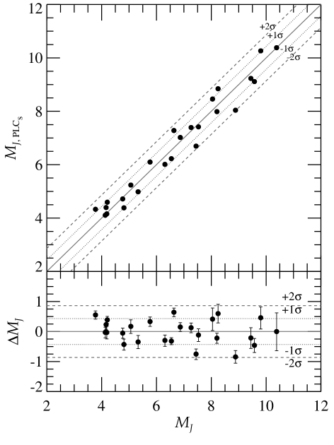
A comparison of the -band absolute magnitudes () estimated using trigonometric parallaxes with those obtained from the PLCs relation () found above is presented in Fig. 1. This figure shows that almost all absolute magnitudes estimated from the PLCs relation are within the 1 limit, and the scatter is not more than 0.9 mag despite large errors of faint objects. In addition, absolute magnitudes estimated from both method are in agreement for short period CVs and there is no systematic effect. A numerical comparison between the PLCs relations found in this study and Ak et al. (2007) can be done using the mean values and standard deviations of the differences , which are calculated -0.005 and 0.403 mag for this study and 0.041 and 0.732 mag for the PLCs relation in Ak et al. (2007). This comparison shows that the PLCs relation suggested in this study gives more reliable results than that in Ak et al. (2007) as the new PLCs relation provides -band absolute magnitudes 2 times more precise compared to those of Ak et al. (2007). We conclude from these comparisons that our PLCs relation can be used to collect a homogeneous sample of CVs regarding to the distances. Reliable Galactic model parameters of CVs can be derived from such a sample.
3 Analysis
3.1 The data sample
In order to obtain a sample of CVs, a preliminary list of the systems whose orbital periods are known and between 82.4 and 720 min is taken from Ritter Kolb (2003, Edition 7.20). The number of CVs in this preliminary sample is 858. However, the number of systems having both 2MASS and observations in this sample is 509. In addition, 196 of these systems were removed because they are beyond the limits of applicability of the PLCs relation found above. Thus, the number of CVs that can be used in this study reduced to 313 and all are listed in an electronic table as a supplement to this paper. In this table, DN denotes dwarf novae, NL nova-like stars, N novae, RN recurrent novae. Polars and intermediate-polars are indicated with P and IP, respectively. In this study, magnetic systems (polars and intermediate polars) were evaluated separately since their evolution may be different from non-magnetic CVs (Townsley & Gänsicke, 2009). Interstellar absorptions in , and bands were estimated using an iterative process described in Ak et al. (2008). De-reddened colours , were calculated as described in Section 2. Finally, absolute magnitudes in -band and distances were estimated from the PLCs relation and Pogson’s equation, respectively.
3.2 Completeness of the sample
Incompleteness of surveys could be often expressed as the reason for disagreements of the results obtained from observational and theoretical studies. Incompleteness of the samples are mostly due to the observational selection effects (Della Valle & Livio, 1996; Aungwerojwit et al., 2005; Gänsicke, 2005; Pretorius et al., 2007b).
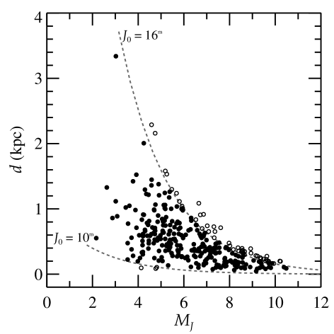
Low-mass transfer rate systems are likely under-represented in the CV samples since systems with rare and low-amplitude outbursts are harder to discover (Patterson, 1998; Pretorius et al., 2007b; Ak et al., 2008). As the theory predicts that the most CVs should be intrinsically faint objects, one of the goals of CV surveys has been to reduce the selection effects by observing the fainter objects. It seems that apparent magnitude limits of surveys are one of the strongest selection effects. Therefore, the completeness limit of the data must be taken into account in a study based on stellar statistics. In order to set a limiting magnitude for the CV sample in this study, the histogram for the de-reddened -band magnitudes () of CVs in the electronic table is shown in Fig. 2. From Fig. 2, the apparent bright and faint limiting -band magnitudes of 10 and 16 mag were selected, respectively, in order to obtain a complete CV sample in a certain volume with the Sun in its centre. By removing systems beyond the limiting magnitudes, the number of CVs drops to 263 from which the Galactic model parameters will be obtained. In Fig. 3, the absolute magnitudes of CVs in the electronic table is plotted against to their distances. Systems between the bright and faint limiting magnitudes are shown with filled circles in Fig. 3, while removed CVs are indicated with open circles.

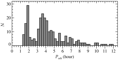
The orbital period distribution of CVs in the final sample is presented in Fig. 4. Among the 263 systems, 124 are nova-like stars, 118 dwarf novae, 14 novae, 6 CVs with unknown type and 1 recurrent nova. There are 73 magnetic CVs (polars and intermediate polars) in this sample. Systems that are not classified as polar or intermediate polar are denoted as non-magnetic systems. Fig. 4 shows that our sample comprises CVs from all orbital period intervals.
The refined sample of 263 CVs in this study is not free from the selection effects. However, selection effects on this sample are likely less than for any sample so far in the literature as the limits defined above make it almost complete in a certain volume. In addition, it is one of the largest CV samples used for deriving the Galactic model parameters available in the literature. Thus, Galactic model parameters of CVs in the Solar neighbourhood derived from this sample should be reliable and useful for CV population models.
3.3 Spatial distribution
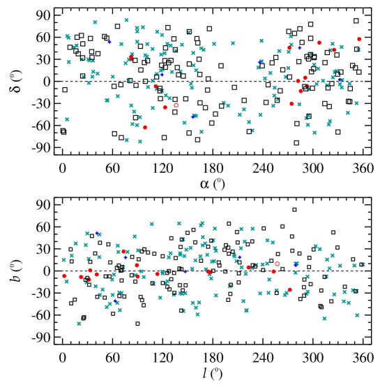
The distribution of CVs according to equatorial (, ) and Galactic coordinates (, ) are plotted in Fig. 5 which indicates that the systems in general are symmetrically distributed about the Galactic plane. The heliocentric rectangular Galactic coordinates ( towards Galactic centre, Galactic rotation, north Galactic Pole) are very useful in order to inspect the Galactic distribution of CVs in the Solar neighbourhood. Thus, the Sun centered rectangular Galactic coordinates of CVs in the sample were calculated and their projected positions on the Galactic plane ( plane) and on a plane perpendicular to it ( plane) are displayed in Fig. 6. The numbers, median distances and median heliocentric Galactic distances of CVs are given in Table 3. Fig. 6 and Table 3 demonstrate that the Galactic positions of CVs in the Solar neighbourhood do not introduce a striking bias for this study, in general. However, it should be noted that the subgroups such as novae (N), recurrent novae (RN) and CVs with unknown type (CV) including only a few members may introduce considerable bias to derivation of the Galactic model parameters for these sub-classes. The numbers, median distances and median heliocentric Galactic distances of CVs above ((h) ) and below ((h) ) the orbital period gap are also given in Table 3. The lower and upper borders for the period gap were adopted from Knigge (2006).
The numbers, median distances and median heliocentric Galactic distances of CVs above ((h) ) and below ((h) ) the period gap are also given in Table 3.
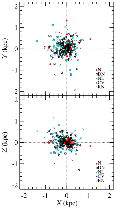
| Type | Number | ||||
| (pc) | (pc) | (pc) | (pc) | ||
| ALL | 263 | 423 | -36 | 59 | 9 |
| h | 59 | 204 | 9 | -24 | 15 |
| h | 185 | 540 | -82 | 102 | 9 |
| DN | 118 | 337 | -13 | 53 | 12 |
| NL | 124 | 528 | -68 | 45 | 15 |
| N | 14 | 720 | 12 | 183 | -24 |
| mCV | 73 | 385 | -56 | 17 | 34 |
| non-mCV | 190 | 458 | -20 | 77 | 2 |
3.4 Galactic model parameters and space density
The number of stars per unit volume is a function of the Galactic positions of stars. Studies based on the deep sky surveys showed that scalelength of the thin-disc stars is larger than 2.6 kpc (Bilir et al., 2006a; Jurić et al., 2008). An inspection of the electronic table shows that the distances of 95 per cent of CVs in the sample are smaller than 1 kpc. This implies that almost all CVs in the sample should be members of the thin-disc component of the Galaxy. Thus, they were not classified according to the population types and estimation of scalelength of CVs were not attempted.
-histograms that exhibit the vertical distribution of objects in the Galaxy must be studied in order to find the Galactic model parameters of the objects in a sample. is the distance of objects from the Galactic plane: where is the Sun’s vertical distance from the Galactic plane (24 pc, Jurić et al., 2008), distance from the Sun and Galactic latitude. Hence, -histograms binned per 100 pc for all CVs (ALL), non-magnetic systems (non-MCV) and magnetic systems (MCV) in the sample are shown in Fig. 7. -histograms of dwarf novae (DN), nova-like stars (NL) and novae (N) are presented in Fig. 8, as well. Although the exponential function has usually been used to describe the number density variation of stars by the distance from the Galactic plane and, thus, to derive the Galactic model parameters, Bilir et al. (2006a, b) showed that observed vertical distribution in the Solar neighbourhood is well-approximated by a secans hyperbolic function. Hence, in order to derive scaleheight and number density of CVs in the Solar neighbourhood, the following two functions were preferred and fitted to -histograms:
| (2) |
and
| (3) |
where is the number of stars in the Solar neighbourhood, and are the exponential and sech2 scaleheights, respectively. By definition, the relation between the exponential and sech2 scaleheight is (Bilir et al., 2006a, b). All error estimates in the analysis were obtained by changing Galactic model parameters until an increase or decrease by 1 in was achieved (Press et al., 1997). The best fits to the -histograms of all CVs in the sample and subgroups are shown in Figs. 7 and 8. The scaleheight and the number of stars in the Solar neighbourhood obtained from the minimum analysis are given in Table 4. In the last column of Table 4, the observed number of CVs with 100 pc () is also listed.


| Subgroup | Function | ||||
|---|---|---|---|---|---|
| ALL | 127 | 213 | 3.45 | 97 | |
| sech2 | 89 | 326 | 7.37 | 97 | |
| DN | 66 | 191 | 5.82 | 49 | |
| sech2 | 47 | 289 | 9.22 | 49 | |
| NL | 47 | 278 | 3.27 | 39 | |
| sech2 | 34 | 404 | 3.42 | 39 | |
| N | 11 | 164 | 1.54 | 7 | |
| sech2 | 9 | 196 | 0.97 | 7 | |
| non-mCV | 84 | 236 | 6.26 | 65 | |
| sech2 | 59 | 356 | 9.03 | 65 | |
| mCV | 44 | 173 | 1.93 | 32 | |
| sech2 | 31 | 264 | 1.97 | 32 |
| Subgroup | Function | ||||
|---|---|---|---|---|---|
| (h) (ALL) | 97 | 135 | 0.39 | 47 | |
| sech2 | 57 | 230 | 1.26 | 47 | |
| non-mCV | 65 | 131 | 0.62 | 31 | |
| sech2 | 37 | 226 | 1.40 | 31 | |
| mCV | 32 | 144 | 0.01 | 16 | |
| sech2 | 19 | 239 | 0.10 | 16 | |
| (h) (ALL) | 41 | 326 | 2.86 | 30 | |
| sech2 | 31 | 444 | 2.58 | 30 | |
| non-mCV | 27 | 364 | 1.72 | 20 | |
| sech2 | 20 | 479 | 1.43 | 20 | |
| mCV | 13 | 305 | 0.28 | 10 | |
| sech2 | 10 | 412 | 0.63 | 10 | |
| (h) (ALL) | 59 | 210 | 0.47 | 38 | |
| sech2 | 39 | 337 | 2.41 | 38 | |
| non-mCV | 35 | 253 | 1.03 | 25 | |
| sech2 | 24 | 390 | 2.46 | 25 | |
| mCV | 23 | 170 | 0.01 | 13 | |
| sech2 | 16 | 250 | 0.01 | 13 | |
| (h) (ALL) | 66 | 192 | 1.65 | 38 | |
| sech2 | 41 | 319 | 2.21 | 38 | |
| non-mCV | 48 | 213 | 0.81 | 30 | |
| sech2 | 31 | 342 | 1.72 | 30 | |
| mCV | 11 | 271 | 0.17 | 8 | |
| sech2 | 8 | 412 | 0.61 | 8 |
Table 4 shows that the exponential function well represents the -histogram constructed for all CVs (ALL) in the sample, dwarf novae (DN), non-magnetic CVs (non-mCV) and magnetic CVs (mCV), with scaleheights of 213, 191, 236 and 173 pc, respectively. However, the -histograms of nova-like stars (NL) and novae (N) are better fitted by the sech2 function which gives scaleheights of 404 and 196 pc, respectively. It should be noted that the number of novae in the sample is too small to draw firm conclusions. Since the exponential function represents the vertical distribution of all CVs in the sample better, a comparison of with for the model distribution produced using this function reveals that there are 308 CVs hiding in the Solar vicinity. Moreover, it is possible to estimate roughly the number of these missing systems in terms of the classes by comparing with obtained from the exponential fits in Table 4: 176 dwarf novae, 84 nova-like stars and 4 novae. We performed Monte Carlo simulations to estimate the contribution of thick-disc CVs in the Solar neighbourhood to the Galactic model parameters since Ak et al. (2013) found that about 6 per cent of CVs in the Solar neighbourhood are members of the thick-disc population in the Galaxy. Assuming that 6, 8 and 10 per cent of CVs in the sample are the thick-disc CVs, our Monte Carlo simulations demonstrate that the effect of these systems to the scaleheights derived above is less than 4 per cent, which can be considered as a negligible contribution.

The Galactic model parameters of CVs classified in terms of the orbital period were derived, as well. In order to define the limits of the orbital period intervals, we divided the CVs in the sample according to almost the same number of systems at four period intervals: 59 systems in the period interval (h) , 59 systems in (h) , 57 systems in (h) and 59 systems in (h) . By this classification, the total number of CVs to be used in deriving the Galactic model parameters drops to 234 as a limiting magnitude of 14 mag was set for CVs with (h) and systems with kpc were ignored to ensure the completeness of the subgroups, while the limiting magnitude of 16 selected above was maintained for CVs in the subgroups with h. Magnetic and non-magnetic systems in these period intervals were also considered as different subgroups. Note that the number of magnetic systems is very small for orbital periods above the orbital period gap. The -histograms of CVs in these subgroups with their best fits are shown in Figs. 9-11. The Galactic model parameters are given in Table 5. The exponential function well represents the -histograms constructed for the CV groups in Figs. 9-11, in general. Table 5 and Figs 9-11 show that the systems with shorter orbital periods ((h) ) have larger scaleheights than CVs in the period range (h) . For the exponential function, the scaleheight increases from 192 to 326 pc while the orbital period decreases from 12 to 2.25 h. However, this trend is broken for the shortest orbital period CVs with h: the scaleheight suddenly decreases to 135 pc for systems with h. A similar trend is also found for the sech2 function. The scaleheight for the sech2 function changes from 319 to 444 pc for CVs with increasing periods in the range (h) , while it drops to 230 pc for CVs with h. The scaleheights estimated from the exponential and sech2 functions for non-magnetic systems (non-mCV) show the same trend as found for all systems in the sample.


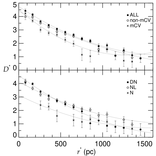
We derived the space density of CVs by dividing the number of stars in consecutive distances from the Sun to the corresponding partial spherical volumes: (Bilir et al., 2006a, b) where is the number of stars in the partial spherical volume which is defined by consecutive distances and from the Sun. The logarithmic space density is expressed . The logarithmic density functions of all CVs, non-magnetic CVs, magnetic CVs, dwarf novae, nova-like stars and novae in the Solar neighbourhood are shown in Fig. 12. In Fig. 12, denotes the centroid distance of the partial spherical volume: . The local space density is the space density estimated for pc. The local space densities obtained for all CVs and subgroups in the sample are listed in Table 6 which shows that the space density of CVs in the Solar neighbourhood is 5.58(1.35) pc-3. Dwarf novae’s (DN) space density is almost the same as found for all CVs in the sample: 4.05(1.27) pc-3. However, the space density of nova-like stars (NL) is only 34 per cent of the space density of DNs. The space density of magnetic (mCV) and non-magnetic CVs (non-mCV) are found to be very similar: 3.13(0.77) and 2.45(0.70) pc-3, respectively. The space densities of CVs in different period intervals are also given in Table 6. Table 6 demonstrates that the space density of CVs in the orbital period intervals above 2.25 h are almost the same with an average value of 0.62 pc-3, while the space density of systems with h is about six times the space density of CVs with h.
| Subgroup | ( pc-3) | Period Interval | ( pc-3) |
|---|---|---|---|
| ALL | 5.58 1.35 | (h) | 3.73 0.12 |
| DN | 4.05 1.27 | (h) | 0.67 0.03 |
| NL | 1.39 0.39 | (h) | 0.64 0.03 |
| N | 0.14 0.10 | (h) | 0.54 0.02 |
| non-mCV | 2.45 0.70 | ||
| mCV | 3.13 0.77 |
3.5 Luminosity function
We defined the luminosity function as the space density of objects in a certain absolute magnitude interval following Bilir et al. (2006a, b). The partial spherical volume including the objects is defined by and distances which correspond to the bright and faint limiting apparent magnitudes of and , respectively, for the absolute magnitude interval in question. The logarithmic luminosity functions are estimated for all systems, dwarf novae, nova-like stars, novae, non-magnetic systems and magnetic systems in the sample and listed in Table 7 and plotted in Fig. 13. An inspection of Table 7 shows that luminosity functions for all subgroups increase towards fainter absolute magnitudes. Table 7 indicates that dwarf novae and nova-like stars have similarly shaped luminosity functions. In addition, similar luminosity functions are also found for non-magnetic and magnetic systems. Novae have a luminosity function rather smaller than those estimated for all the subgroups.

| All Systems | Dwarf novae | Nova-like Stars | Novae | non-Magnetic CVs | Magnetic CVs | |||||||||
|---|---|---|---|---|---|---|---|---|---|---|---|---|---|---|
| N | N | N | N | N | N | |||||||||
| (1.5, 2.5] | 398–6310 | 1.05(E12) | 1 | — | - | — | 1 | — | - | — | 1 | — | - | — |
| (2.5, 3.5] | 251–3981 | 2.64(E11) | 6 | -10.641.90 | 2 | -11.123.40 | 3 | -10.942.70 | 1 | -11.425.00 | 6 | -10.641.90 | - | — |
| (3.5, 4.5] | 158–2512 | 6.64(E10) | 36 | -9.270.70 | 10 | -9.821.40 | 23 | -9.460.90 | 2 | -10.523.20 | 28 | -9.370.70 | 8 | -9.920.70 |
| (4.5, 5.5] | 100–1585 | 1.67(E10) | 67 | -8.400.40 | 17 | -8.990.90 | 43 | -8.590.60 | 5 | -9.521.80 | 49 | -8.530.40 | 18 | -8.970.40 |
| (5.5, 6.5] | 63–1000 | 4.19(E9) | 46 | -7.960.50 | 21 | -8.300.80 | 21 | -8.300.80 | 2 | -9.322.90 | 35 | -8.080.50 | 11 | -8.580.50 |
| (6.5, 7.5] | 40–631 | 1.05(E9) | 52 | -7.310.40 | 31 | -7.530.60 | 15 | -7.850.90 | 4 | -8.421.80 | 40 | -7.420.40 | 12 | -7.940.40 |
| (7.5, 8.5] | 25–398 | 2.64(E8) | 30 | -6.940.60 | 19 | -7.140.70 | 11 | -7.381.00 | - | — | 16 | -7.220.60 | 14 | -7.280.60 |
| (8.5, 9.5] | 16–251 | 6.62(E7) | 20 | -6.520.60 | 14 | -6.670.80 | 6 | -7.041.20 | - | — | 12 | -6.740.60 | 8 | -6.920.60 |
| (9.5, 10.5] | 10–158 | 1.65(E7) | 5 | -6.521.20 | 4 | -6.621.40 | 1 | -7.223.10 | - | — | 3 | -6.741.30 | 2 | -6.921.30 |
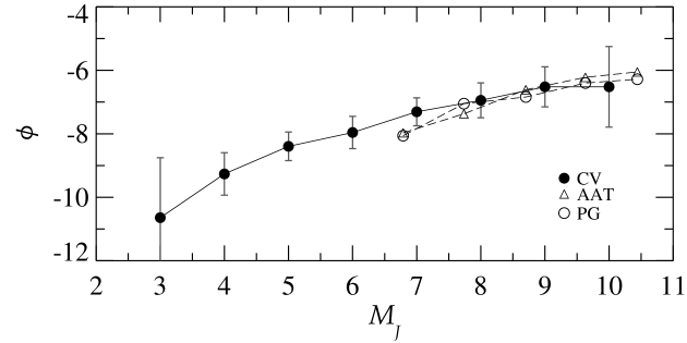
For a comparison of the luminosity function of DA white dwarfs found from the Anglo Australian Telescope survey (AAT, Boyle, 1989) and Palomar Green survey (PG, Fleming et al., 1986) with the luminosity function of CVs derived in this study, the Johnson absolute magnitudes of CVs are transformed to 2MASS absolute magnitudes using Padova Isochrones (Bressan et al., 2012). Since the spatial distribution of CVs in Fig. 6 shows that these systems belong to the old thin disc of the Galaxy, in general, an analytical relation between and by assuming a mass fraction of metals of , a logarithmic surface gravity of and a mean age of Gyr (Ak et al., 2010) are obtained in the selection of isochrones. The comparison of the luminosity functions of DA white dwarfs and CVs in the sample is shown in Fig. 14. The analysis show that the best fits between the luminosity functions of CVs and white dwarfs are obtained by dividing the luminosity functions of white dwarfs a factor of 450 and 350 for the PG and AAT surveys, respectively.
4 Conclusions
In order to derive the spatial distribution, Galactic model parameters and luminosity function of CVs, a new PLCs relation has been obtained using the 2MASS and photometries. This new PLCs relation gives more reliable results than that in Ak et al. (2007). A CV sample was collected using the new PLCs relation. The sample was limited in terms of the -band magnitudes to ensure its completeness. The Galactic model parameters, space densities and luminosity functions derived in this study can be used to constrain the population models of CVs. Our conclusions can be summarized as follows:
-
•
Estimated distances to the Sun are smaller than 1 kpc for CVs in the sample. CVs in the Solar neighbourhood are located in the thin-disc with distances lower than 700 pc, in general, a result consistent with (Ak et al., 2013).
-
•
The exponential scaleheight of CVs in the sample is 213 pc. This value is in agreement with the exponential scaleheights of 190 and 160-230 pc suggested by Patterson (1984) and van Paradijs et al. (1996), respectively. However, it is considerably larger than the exponential scaleheight of 15814 pc derived by Ak et al. (2008).
-
•
If the -distribution of all CVs in the sample is modeled by a sech2 function (Bilir et al., 2006a, b), the scaleheight of CVs in the Solar neighbourhood is derived 326 pc. This scaleheight seems to be acceptable as Gänsicke et al. (2009) concluded that the scaleheight of CVs is very likely larger than the 190 pc found by Patterson (1984). Moreover, Pretorius et al. (2007b) argues that the 190 pc used by Patterson (1984) can be suitable only for youngest CVs. This is a very plausible argument since the previous measurements for the scaleheight of CVs were based on the samples which are strongly biased towards bright objects and these measurements were made using only the exponential function. Thus, we suggest that the scaleheight of CVs in the Solar vicinity should be 330 pc and that the sech2 function should be also considered in the CV population models. However, it must be keep in mind that the bias of the bright CVs in the sample can be dominant on the derivation of observational Galactic model parameters.
-
•
Our analysis show that the systems with short orbital periods (2.25-3.7h) have larger scaleheights than that estimated for CVs with h. Also, it seems that the observational scaleheights derived in this study are not in agreement with the scaleheights adopted by Pretorius et al. (2007b). The trend of the scaleheight in terms of the orbital period encourages us to predict that the exponential and sech2 scaleheights of the CVs with h are larger than 326 and 444 pc, respectively, even though the observed scale height of these (faint) systems is much smaller.
-
•
The logarithmic density functions of CVs show that the density functions derived in this study is in agreement with those shown in Ak et al. (2008). We found that the space density of CVs in the Solar neighbourhood is 5.58(1.35) pc-3, a result consistent with (Warner, 1974; Patterson, 1984, 1998; Ringwald, 1993; Schwope et al., 2002a; Araujo-Betancor et al., 2005; Pretorius et al., 2007a; Ak et al., 2008; Revnivtsev et al., 2008; Pretorius & Knigge, 2012; Pretorius et al., 2013). However, the predicted values in the population synthesis studies are pc-3 (Ritter & Burkert, 1986; de Kool, 1992; Kolb, 1993; Politano, 1996; Willems et al., 2005, 2007). Although we used a fairly complete data sample, this comparison shows that there is still not a satisfactory agreement between the observational and predicted space densities of CVs.
-
•
Space densities of the CVs with h in the Solar neighbourhood are almost the same: 0.62 pc-3, in average. However, the space density of CVs with the orbital periods shorter than 2.25 h is about 6 times larger than that derived for longer period CVs. This result indicates that the faintest systems with distances greater than 200 pc could not be observed yet.
-
•
Although it is not clear if masses of the white dwarfs in CVs are similar to those of isolated DA white dwarfs (Sion, 1999), our analysis based on the comparisons of the luminosity function of DA white dwarfs (Fig. 14) found from the AAT survey (Boyle, 1989) and the PG survey (Fleming et al., 1986) with the luminosity function of CVs show that the best fits are obtained by dividing the luminosity functions of white dwarfs by 450 and 350 for the PG and AAT surveys, respectively.
5 Acknowledgments
This work has been supported in part by the Scientific and Technological Research Council of Turkey (TÜBİTAK) 212T091. This work has been supported in part by Istanbul University: Project number 27839. We thank the anonymous referee for a through report and useful comments that helped improving an early version of the paper. This research has made use of the Wide-field Infrared Survey Explorer and NASA/IPAC Infrared Science Archive and Extragalactic Database (NED), which are operated by the Jet Propulsion Laboratory, California Institute of Technology, under contract with the National Aeronautics and Space Administration. This publication makes use of data products from the Two Micron All Sky Survey, which is a joint project of the University of Massachusetts and the Infrared Processing and Analysis Center/California Institute of Technology, funded by the National Aeronautics and Space Administration and the National Science Foundation. This research has made use of the SIMBAD, and NASA’s Astrophysics Data System Bibliographic Services.
References
- Ak et al. (2007) Ak, T., Bilir, S., Ak, S., Retter, A., 2007. NewA 12, 446.
- Ak et al. (2008) Ak, T., Bilir, S., Ak, S., Eker, Z., 2008. NewA 13, 133.
- Ak et al. (2010) Ak, T., Bilir, S., Ak, S., Coşkunoğlu, K.B., Eker, Z., 2010. NewA 15, 491.
- Ak et al. (2013) Ak, T., Bilir, S., Güver, T., Çakmak, H., Ak, S., 2013. NewA 22, 7.
- Araujo-Betancor et al. (2005) Araujo-Betancor, S.,Gänsicke, B.T., Long, K.S., Beuermann, K., de Martino, D., Sion, E.M., Szkody, P., 2005. ApJ 622, 589.
- Aungwerojwit et al. (2005) Aungwerojwit, A. et al., 2005. A&A 443, 995.
- Bailey (1981) Bailey, J., 1981. MNRAS 197, 31.
- Barnes & Evans (1976) Barnes, T.G., Evans, D.S., 1976. MNRAS 174, 489.
- Berriman et al. (1985) Berriman, G., Szkody, P., Capps, R.W., 1985. MNRAS 217, 327.
- Beuermann (2006) Beuermann, K., 2006. A&A 460, 783.
- Beuermann et al. (1998) Beuermann, K., Baraffe, I., Kolb, U., Weichhold, M., 1998. A&A 339, 518.
- Beuermann et al. (2003) Beuermann, K., Harrison, Th.E., McArthur, B.E., Benedict, G.F., Gänsicke, B.T., 2003. A&A 412, 821.
- Beuermann et al. (2004) Beuermann, K., Harrison, T.E., McArthur, B.E., Benedict, G.F., Gänsicke, B.T., 2004. A&A 419, 291.
- Bilir et al. (2006a) Bilir, S., Karaali, S., Ak, S., Yaz, E., Hamzaoğlu, E., 2006a. NewA 12, 234.
- Bilir et al. (2006b) Bilir, S., Karaali, S., Gilmore, G., 2006b. MNRAS 366, 1295.
- Bilir et al. (2011) Bilir, S., Karaali, S., Ak, S., Dağtekin, N.D., Önal, Ö., Yaz, E., Coşkunoğlu, B., Cabrera-Lavers, A., 2011. MNRAS 417, 2230.
- Boyle (1989) Boyle, B.J., 1989. MNRAS 240, 549.
- Bressan et al. (2012) Bressan, A., Marigo, P., Girardi, L., Salasnich, B., Dal Cero, C., Rubele, S., Nanni, A., 2012. MNRAS 427, 127.
- Byckling et al. (2010) Byckling, K., Mukai, K., Thorstensen, J.R., Osborne, J.P., 2010. MNRAS 408, 2298.
- Cardelli et al. (1989) Cardelli, J.A., Clayton, G.C., Mathis, J.S., 1989. ApJ 345, 245.
- Cutri et al. (2003) Cutri, R.M. et al., 2003. VizieR On-line Data Catalog: II/246. Originally published in: University of Massachusetts and Infrared Processing and Analysis Center, (IPAC/California Institute of Technology).
- Cutri et al. (2012) Cutri, R.M. et al., 2012. All-Sky Data Release, VizieR Online Data Catalog, 2311.
- de Kool (1992) de Kool, M., 1992. A&A 261, 188.
- Della Valle & Livio (1996) Della Valle, M., Livio, M., 1996. ApJ 457, L77.
- Duerbeck (1984) Duerbeck, H.W., 1984. Ap&SS 99, 363.
- Duerbeck (1999) Duerbeck, H.W., 1999. IBVS No.4731, 1.
- Fiorucci & Munari (2003) Fiorucci, M., Munari, U., 2003. A&A 401, 781.
- Fleming et al. (1986) Fleming, T.A., Liebert, J., Green, R.F., 1986. ApJ 308, 176.
- Fu et al. (2004) Fu, H., Li, Z.-Y., Leung, K.-C, Zhang, Z.-S., Li, Z.-L., Gaskell, C.M., 2004. Chinese J. Astron. Astrophys. 4, 88.
- Gariety & Ringwald (2012) Gariety, M.J., Ringwald, F.A., 2012. NewA 17, 154.
- Gänsicke (2005) Gänsicke, B.T., 2005. in The Astrophysics of Cataclysmic Variables and Related Objects, ASP Conf. Ser., Vol. 330, J.-M. Hameury, J.-P. Lasota eds., 3.
- Gänsicke et al. (2009) Gänsicke, B.T., et al., 2009. MNRAS 397, 2170.
- Hameury et al. (1988) Hameury, J.M., King, A.R., Lasota, J.P., Ritter, H., 1988. ApJ 327, 77.
- Harrison et al. (2004) Harrison, T.E., Johnson, J.J., McArthur, B.E., Benedict, G.F., Szkody, P., Howell, S.B., Gelino, D.M., 2004. AJ 127, 460.
- Harrison et al. (2009) Harrison, T.E., Bornak, J., Howell, S.B., Mason, E., Szkody, P., McGurk, R., 2009. AJ 137, 4061.
- Harrison et al. (2013) Harrison, T.E., et al., 2013. AJ 145, 19.
- Hellier (2001) Hellier, C., 2001. Cataclysmic Variable Stars, How and why they vary. Springer-Praxis Books in Astronomy and Space Sciences, Cornwall, UK.
- Jurić et al. (2008) Jurić, M., et al., 2008. ApJ 673, 864.
- King (1988) King, A.R., 1988. QJRAS 29, 1.
- Knigge (2006) Knigge, C., 2006. MNRAS 373, 484.
- Knigge (2007) Knigge, C., 2007. MNRAS 382, 1982.
- Knigge (2011) Knigge, C., 2011. Evolution of compact binaries. ASP Conference Proceedings, Vol. 447, Linda Schmidtobreick, Matthias R. Schreiber, and Claus Tappert (eds.), 3.
- Kolb (1993) Kolb, U., 1993. A&A 271, 149.
- McArthur et al. (1999) McArthur, B.E., Benedict, G.F., Lee, J., Lu, C.-L., van Altena, W.F. et al., 1999. ApJ 520, L59.
- McArthur et al. (2001) McArthur, B.E., Benedict, G.F., Lee, J., van Altena, W.F., Slesnick, C.L., et al., 2001. ApJ 560, 907.
- Patterson (1984) Patterson, J., 1984. ApJS 54, 443.
- Patterson (1998) Patterson, J., 1998. PASP 110, 1132.
- Patterson et al. (2005) Patterson, J., et al., 2005. PASP 117, 1204.
- Patterson et al. (2008) Patterson, J., Thorstensen, J.R., Knigge, C., 2008. PASP 120, 510.
- Politano (1996) Politano, M., 1996. ApJ 465, 338.
- Press et al. (1997) Press, W.H., Teukolsky, S.A., Vetterling, W.T., Flannery, B.P., 1997. Numerical Recipes in Fortran 77 - The Art of Scientific Computing, Second Edition, ISBN 0-521-43064-X, Cambridge Univ. Press., 688.
- Pretorius et al. (2007a) Pretorius, M.L., Knigge, C., O’Donoghue, D., Henry, J.P., Gioia, I.M., Mullis, C.R., 2007a. MNRAS 382, 1279.
- Pretorius et al. (2007b) Pretorius, M.L., Knigge, C., Kolb, U., 2007b. MNRAS 374, 1495.
- Pretorius & Knigge (2012) Pretorius, M.L., Knigge, C., 2012. MNRAS 419, 1442.
- Pretorius et al. (2013) Pretorius, M.L., Knigge, C., Schwope, A.D., 2013. MNRAS 432, 570.
- Revnivtsev et al. (2008) Revnivtsev, M., Lutovinov, A., Churazov, E., Sazonov, S., Gilfanov, M., Grebenev, S., Sunyaev, R., 2008. A&A, 491, 209.
- Ringwald (1993) Ringwald, F.A., 1993. PASP 105, 805.
- Ritter (2012) Ritter, H., 2012. MmSAI 83, 505.
- Ritter & Burkert (1986) Ritter, H., Burkert, A., 1986. A&A 158, 161.
- Ritter & Kolb (2003) Ritter H., Kolb U., 2003. A&A 404, 301 (update RKcat7.20, 2013).
- Sazonov et al. (2006) Sazonov, S., Revnivtsev, M., Gilfanov, M., Churazov, E., Sunyaev, R., 2006. A&A 450, 117.
- Schlafly & Finkbeiner (2011) Schlafly, E.F., Finkbeiner, D.P., 2011. ApJ 737, 103.
- Schlegel et al. (1998) Schlegel, D.J., Finkbeiner, D.P., Davis, M., 1998. ApJ 500, 525.
- Schmidt et al. (2005) Schmidt, G.D., et al., 2005, ApJ 630, 1037.
- Schwope et al. (2002a) Schwope, A.D., Brunner, H., Buckley, D., Greiner, J., Heyden, K.V.D., Neizvestny, S., Potter, S., Schwarz, R., 2002a. A&A 396, 895.
- Schwope et al. (2002b) Schwope, A.D., Brunner, H., Hambaryan, V., Schwarz, R., 2002b. The Physics of Cataclysmic Variables and Related Objects, ASP Conference Proceedings, Vol. 261, B.T. Gänsicke, K. Beuermann, and K. Reinsch (eds.), 102.
- Skrutskie et al. (2006) Skrutskie, M.F., et al., 2006. AJ 131, 1163.
- Sion (1999) Sion, E.M., 1999. PASP 111, 532.
- Smith (2007) Smith, R.C., 2007. arXiv:astro-ph/0701654.
- Sproats et al. (1996) Sproats, L.N., Howell, S.B., Mason, K.O., 1996. MNRAS 282, 1211.
- Spruit & Ritter (1983) Spruit, H.C., Ritter, H., 1983. A&A 124, 267.
- Thorstensen (2003) Thorstensen, J.R., 2003. AJ 126, 3017.
- Thorstensen et al. (2008) Thorstensen, J.R., Lépine, S., Shara, M., 2008. AJ 136, 2107.
- Thorstensen et al. (2009) Thorstensen, J.R., et al., 2009. PASP 121, 465.
- Townsley & Gänsicke (2009) Townsley, D.M., Gänsicke, B.T., 2009. ApJ 693, 1007.
- van Altena et al. (1995) van Altena, W.F., Lee, J.T., Hoffleit, D., 1995. VizieR On-line Data Catalog: I/174.
- van Leeuwen (2007) van Leeuwen, F., 2007. A&A 474, 653.
- van Paradijs et al. (1996) van Paradijs, J., Augusteijn, T., Stehle, R., 1996. A&A 31, 93.
- Warner (1974) Warner, B., 1974. MNSSA 33, 21.
- Warner (1995) Warner, B., 1995. Cataclysmic Variable Stars. Cambridge University Press, Cambridge.
- Willems et al. (2005) Willems, B., Kolb, U., Sandquist, E.L., Taam, R.E., Dubus, G., 2005. ApJ 635, 1263.
- Willems et al. (2007) Willems, B., Kolb, U., Sandquist, E.L., Taam, R.E., Dubus, G., 2007. ApJ 657, 465.
- Wright et al. (2010) Wright, E.L., et al., 2010. AJ 140, 1868.
- Yaz Gökçe et al. (2013) Yaz Gökçe, E., Bilir, S., Öztürkmen, N.D., Duran, Ş., Ak, T., Ak, S., Karaali, S., 2013. NewA 25, 19.