How Well Can Future CMB Missions Constrain Cosmic Inflation?

Abstract

We study how the next generation of Cosmic Microwave Background (CMB) measurement missions (such as EPIC, LiteBIRD, PRISM and COrE) will be able to constrain the inflationary landscape in the hardest to disambiguate situation in which inflation is simply described by single-field slow-roll scenarios. Considering the proposed PRISM and LiteBIRD satellite designs, we simulate mock data corresponding to five different fiducial models having values of the tensor-to-scalar ratio ranging from $10^{-1}$ down to $10^{-7}$. We then compute the Bayesian evidences and complexities of all Encyclopædia Inflationaris models in order to assess the constraining power of PRISM alone and LiteBIRD complemented with the Planck 2013 data. Within slow-roll inflation, both designs have comparable constraining power and can rule out about three quarters of the inflationary scenarios, compared to one third for Planck 2013 data alone. However, we also show that PRISM can constrain the scalar running and has the capability to detect a violation of slow roll at second order. Finally, our results suggest that describing an inflationary model by its potential shape only, without specifying a reheating temperature, will no longer be possible given the accuracy level reached by the future CMB missions.

1 Introduction

Primordial gravity waves could play a crucial role in our attempts to learn about the early Universe. They are a generic prediction of inflation and their amplitude, described by the tensor-to-scalar ratio $r$, carries precious information about the energy scale of inflation. The observational situation of $r$, however, is at the time of writing, unclear. The Cosmic Microwave Background (CMB) Planck data puts an upper bound on $r$ (the precise value of which depends on the assumptions made on the power spectra and on the priors; in a minimal set up, one obtains $r\lesssim 0.11$) while the BICEP2 measurement of the $B$-mode angular power spectrum would imply $r=0.16^{+0.06}_{-0.05}$ [1, 2]. This last value is currently debated and needs to be confirmed in view of the role played by polarized foregrounds [3, 4, 5]. In this respect, the next release of the Planck data will be of crucial importance, in particular in order to assess the compatibility of these two data sets.

Recently, different CMB missions have been proposed and, among other results, are expected to provide unprecedented constraints on $r$. This includes the Experimental Probe of Inflationary Cosmology (EPIC) [6], the Lite satellite for the studies of B-mode polarization and Inflation from cosmic background Radiation Detection (LiteBIRD) [7], the Polarized Radiation Imaging and Spectroscopy Mission (PRISM) [8] and the Cosmic Origins Explorer (COrE) [9]. These missions have different designs and goals but, roughly speaking, they would allow a measurement of a tensor-to-scalar ratio down to $r\simeq 10^{-3}$ (without assuming delensing [10, 11]). It seems therefore worth studying to which extent such a measurement could improve our knowledge of inflation compared to what has already been established with the Planck data [12, 13]. In particular, it is interesting to consider “the hardest to disambiguate situation” in which inflation is well described by minimal single-field slow-roll models. In this situation, which is the one favored by Planck 2013, there is no entropy perturbations in the CMB, non-Gaussianities remain unobservable while the primordial power spectra are featureless [14]. We choose to focus on this case since this is the most difficult and conservative situation one can imagine. Indeed, if realized, we won’t be able to use the observables mentioned before to narrow down the inflationary landscape. In other words, if non-vanilla properties are detected by future missions, it could only improve our ability to test and constrain inflation and, therefore, the results discussed here represent what can be done in the “worst case scenario”.

In quantitative terms, the performance of a model, given a data set, can be measured by calculating its Bayesian evidence [15, 16, 17, 18]. For all the Encyclopædia Inflationaris models [19], which currently achieve the best compromise between quality of the fit and simplicity of the theoretical description (since, as already mentioned, we do not observe entropy mode and/or non-Gaussianities), Bayes factors have been recently computed for the Planck data in Refs. [13, 20] and for the BICEP2 data in Ref. [21]. A way to discuss the constraining power of an experiment in this context is to use the Jeffreys’ scale and count the number of models in the “inconclusive”, “weak evidence”, “moderate evidence” and “strong evidence” zones with respect to the best model. For instance, from the Planck data, one finds $26\%$ of the models in the first category (corresponding to $17$ different shapes of the potential), $21\%$ in the second, $17\%$ in the third, and $34\%$ in the fourth and last one. These numbers can be further improved in one uses the Bayesian complexity as another statistical indicator [22]. Of course, the Jeffreys’ scale is indicative only, although it is usually considered that models belonging to the strong evidence category can really be considered as “ruled out”, but the way the inflationary scenarios are distributed among the Jeffreys’ categories for different experiments gives a fair view of their constraining power.

Satellite	$C_{\mathrm{noise}}^{\mathrm{T}}$	$C_{\mathrm{noise}}^{\mathrm{E}}$	$C_{\mathrm{noise}}^{\mathrm{B}}$	$\theta_{\mathrm{fwhm}}$	$f_{\mathrm{sky}}$
PRISM	$5\times 10^{-7}\,\mathrm{\mu K}^{2}$	$2C_{\mathrm{noise}}^{\mathrm{T}}$	$2C_{\mathrm{noise}}^{\mathrm{T}}$	$3.2^{\prime}$	$0.7$
LiteBIRD	$7\times 10^{-7}\,\mathrm{\mu K}^{2}$	$2C_{\mathrm{noise}}^{\mathrm{T}}$	$2C_{\mathrm{noise}}^{\mathrm{T}}$	$38.5^{\prime}$	$0.7$

Table 1: The two idealized CMB missions considered in this paper. They match the optimal specifications of LiteBIRD and PRISM and should be representative of other similar proposed designs (see text).

In this work, we simulate mock data for five fiducial models and two representative future CMB missions corresponding to the idealized design of LiteBIRD and PRISM (see Table 1). Then, using the pipeline described in Refs. [23, 13, 20], we compute the Bayesian evidences of all Encyclopædia Inflationaris models and their distribution among the Jeffreys’ categories for the two missions quoted before. This is our main result and it is displayed in Fig. 6.

This article is organized as follows. In the next section, Sec. 2, we describe the method used while the results are presented in Sec. 3, namely the percentage of models in each Jeffreys’ categories for LiteBIRD and PRISM. Finally, the implications for inflation and future strategies are discussed in the conclusion in Sec. 4.

2 Methodology

The cosmological model that we consider is an inflationary flat $\Lambda$CDM scenario. It is characterized by the parameters $\theta=\{\theta_{\mathrm{s}},\theta_{\mathrm{reh}},\theta_{\mathrm{inf}}\}$ where the quantities $\theta_{\mathrm{s}}$, given by $\theta_{\mathrm{s}}\equiv\{\Omega_{\mathrm{b}}h^{2},\Omega_{\mathrm{dm}}h^{2},\tau,100\theta_{{\scriptscriptstyle{\mathrm{MC}}}}\}$ (respectively, the baryons normalized density, the cold dark matter normalized density, the optical depth and an angle related to the angular size of the sound horizon on the last scattering surface; $h$ being the reduced Hubble parameter), describe post-inflationary physics, the $\theta_{\mathrm{reh}}$’s describe the reheating phase and the $\theta_{\mathrm{inf}}$’s are inflationary parameters describing the shape of the inflaton potential [24, 25]. The initial power spectra for density perturbations and primordial gravity waves are given by formulas derived in the slow-roll approximation, i.e. a scale-invariant piece plus small scale dependent logarithmic corrections [26, 27]. As a consequence, they depend on the parameter $P_{*}$, describing the overall normalization of the primordial fluctuations and three slow-roll parameters (at second order in slow roll) evaluated at Hubble radius crossing during inflation, $\epsilon_{1}$, $\epsilon_{2}$ and $\epsilon_{3}$; for explicit formulas, see for instance Refs. [28, 29, 19]. The dependence on specific inflationary scenarios lies in the fact that $\epsilon_{n}=\epsilon_{n}\left(\theta_{\mathrm{inf}},\theta_{\mathrm{reh}}\right)$.

Fiducial model	Potential $V(\phi)/M^{4}$	Potential parameters
$\mathrm{LFI}_{\mathrm{fid}}$	$\left(\phi/M_{\scriptscriptstyle{\mathrm{Pl}}}\right)^{2}$
$\mathrm{DWI}_{\mathrm{fid}}$	$\left[(\phi/\phi_{{}_{0}})^{2}-1\right]^{2}$	$\phi_{{}_{0}}/M_{\scriptscriptstyle{\mathrm{Pl}}}=25$
$\mathrm{HI}_{\mathrm{fid}}$	$\left[1-\exp\left(-\sqrt{2/3}\phi/M_{\scriptscriptstyle{\mathrm{Pl}}}\right)\right]^{2}$
$\mathrm{ESI}_{\mathrm{fid}}$	$1-\exp\left(-q\frac{\phi}{M_{\scriptscriptstyle{\mathrm{Pl}}}}\right)$	$q=8$
$\mathrm{MHI}_{\mathrm{fid}}$	$1-\operatorname{sech}\left(\phi/\mu\right)$	$\mu/M_{\scriptscriptstyle{\mathrm{Pl}}}=0.01$

Table 2: The five fiducial models used to generate the mock data and the corresponding potential parameters value. The post-inflationary cosmological parameters have been fixed to typical values compatible with the Planck 2013 data, namely $\Omega_{\mathrm{b}}h^{2}\equiv 0.0223$, $\Omega_{\mathrm{dm}}h^{2}\equiv 0.120$, $\Omega_{\nu}h^{2}\equiv 6.45\times 10^{-4}$, $\tau\equiv 0.0931$ and $h\equiv 0.674$. The reheating temperature has been set to $T_{\mathrm{reh}}\equiv 10^{8}\,\mathrm{GeV}$ with a reheating mean equation of state $\overline{w}_{\mathrm{reh}}\equiv 0$ and a primordial amplitude for the scalar perturbations $P_{*}\equiv 2.203\times 10^{-9}$.

Fiducial model	$\epsilon_{1}$	$\epsilon_{2}$	$\epsilon_{3}$	$n_{\scriptscriptstyle{\mathrm{S}}}$	$r$
$\mathrm{LFI}_{\mathrm{fid}}$	$9.63\times 10^{-3}$	$1.93\times 10^{-2}$	$1.93\times 10^{-2}$	$0.961$	$1.52\times 10^{-1}$
$\mathrm{DWI}_{\mathrm{fid}}$	$5.40\times 10^{-3}$	$2.77\times 10^{-2}$	$1.41\times 10^{-2}$	$0.962$	$8.45\times 10^{-2}$
$\mathrm{HI}_{\mathrm{fid}}$	$2.65\times 10^{-4}$	$3.81\times 10^{-2}$	$1.93\times 10^{-2}$	$0.961$	$4.12\times 10^{-3}$
$\mathrm{ESI}_{\mathrm{fid}}$	$3.28\times 10^{-6}$	$4.10\times 10^{-2}$	$2.05\times 10^{-2}$	$0.959$	$5.09\times 10^{-5}$
$\mathrm{MHI}_{\mathrm{fid}}$	$2.19\times 10^{-8}$	$4.19\times 10^{-2}$	$2.09\times 10^{-2}$	$0.958$	$3.40\times 10^{-7}$

Table 3: Fiducial values for the slow-roll parameters, the spectral index and the tensor-to-scalar ratio (at the pivot scale $k_{*}=0.05\,\mathrm{Mpc}^{-1}$) for the five fiducial models used to generate the mock data (see Table. 2).

Let us now present the line of reasoning used in this article. The first step has been to generate mock data. We have chosen to analyze five different situations, associated with five fiducial models summarized in table 2.

The first one corresponds to a case where B-modes should easily be detected by the future experiments because the underlying model is compatible with the BICEP2 value, $r\simeq 0.16$. To model this case, we have chosen a fiducial slow-roll inflationary scenario given by the quadratic Large Field model $m^{2}\phi^{2}/2$ ($\mathrm{LFI}_{2}$ in the Encyclopædia Inflationaris terminology). The second case is supposed to describe a situation where the estimated value of the tensor-to-scalar ratio is smaller than the BICEP2 value due to a possible re-estimation of the polarized foregrounds contribution, say $r\simeq 0.08$ [3, 4]. To describe this case, we have considered a Double Well inflation scenario ($\mathrm{DWI}$) with $\phi_{{}_{0}}/M_{\scriptscriptstyle{\mathrm{Pl}}}\equiv 25$. The third situation corresponds to a case where one is close to the detection limit of $r$ and we use the Starobinsky (or Higgs) inflation model ($\mathrm{HI}$) to parametrize this situation. The fourth example is chosen such that the tensor-to-scalar ratio is less than the threshold value $r=10^{-3}$ and we consider an Exponential Supersymmetric scenario ($\mathrm{ESI}$) with $q\equiv 8$. Finally, the fifth and last case corresponds to a situation where the fiducial model is associated with an undetectable amount of primordial gravity waves. To describe this possibility, we have chosen a Mutated Hilltop inflation model ($\mathrm{MHI}$) with $\mu\equiv 0.01M_{\scriptscriptstyle{\mathrm{Pl}}}$ (see Ref. [19] for more details on these models).

Moreover, all fiducial models share the same reheating and cosmological parameters. The reheating temperature has been fixed to $T_{\mathrm{reh}}\equiv 10^{8}\,\mathrm{GeV}$ with a mean equation of state $\overline{w}_{\mathrm{reh}}\equiv 0$ while the post-inflationary evolution is assumed to be described by a flat $\Lambda$CDM model with $\Omega_{\mathrm{b}}h^{2}\equiv 0.0223$, $\Omega_{\mathrm{dm}}h^{2}\equiv 0.120$, $\Omega_{\nu}h^{2}\equiv 6.45\times 10^{-4}$, $\tau\equiv 0.0931$ and $h\equiv 0.674$. For each fiducial model, the first three Hubble flow functions have been calculated using the ASPIC library and they are given in table 3. For each model, the ASPIC code solves the reheating consistent slow-roll equations to get the field value at which the pivot scale $k_{*}$ crossed the Hubble radius during inflation, and then the corresponding values for the Hubble flow functions (see section 2.2 in Ref. [19]). At last, we have used a modified version of the CAMB code to generate the fiducial temperature and polarization multipole moments [30].

Once these mock data have been generated, the next step is to analyze them from the point of view of the two CMB missions under focus and this requires to specify their likelihood function. For this purpose, assuming Gaussian statistics, one can show that the likelihood function $\mathcal{L}\left[C_{\ell}^{\mathrm{mock}}|C_{\ell}^{\mathrm{th}}\left(\theta_{\mathrm{s}},\theta_{\mathrm{reh}},\theta_{\mathrm{inf}}\right),\Sigma\right]$ over the full sky is given by a Wishart distribution [31, 32, 33, 34]. Here $C_{\ell}^{\mathrm{mock}}$ and $C_{\ell}^{\mathrm{th}}$ stand for the mock and theoretical angular power spectra, respectively. These distributions are different for the two experiments under scrutiny, PRISM and LiteBIRD, due to their different specifications and this is encoded in the quantity $\Sigma\equiv\{C_{\mathrm{noise}}^{\mathrm{T}},C_{\mathrm{noise}}^{\mathrm{E}},C_{\mathrm{noise}}^{\mathrm{B}},\theta_{\mathrm{fwhm}},f_{\mathrm{sky}}\}$. The noise power $C_{\mathrm{noise}}$ for temperature and polarization, the full width at half maximum (fwhm) $\theta_{\mathrm{fwhm}}$ for the (assumed) Gaussian beam and fraction of sky coverage $f_{\mathrm{sky}}$ are summarized in Table 1. As can be seen in this table, the LiteBIRD beam resolution is relatively poor, by design, and as such, we have complemented the LiteBIRD forecast with the Planck 2013 data.

In order to carry out a Bayesian analysis, one must specify the priors. Here, we have chosen the same priors on $\theta_{\mathrm{s}}$, $\theta_{\mathrm{reh}}$ and $\theta_{\mathrm{inf}}$ than those discussed at length in Refs. [13, 21]. Bayesian evidences and complexities are then derived by performing a data analysis for each experiment and each fiducial model by using all the model of Encyclopædia Inflationaris. Moreover, we have assumed uninformative priors between the different models $\mathcal{M}_{i}$, that is to say $\pi(\mathcal{M}_{i})=1/N^{{\scriptscriptstyle{\mathrm{mod}}}}$, where $N^{{\scriptscriptstyle{\mathrm{mod}}}}$ is the number of Encyclopædia Inflationaris scenarios that we consider. In practice, we have followed the same method as described in Refs. [23, 13, 21] which involves the derivation of an effective marginalized likelihood function depending only on the reheating and primordial parameters. All evidences have been derived using the MultiNest nested sampling algorithm [35, 36, 37] with a target accuracy of $10^{-4}$ and a number a live points equals to $30000$.

In the following section, we report the results that have been obtained for all the Encyclopædia Inflationaris scenarios. To make the comparison with the current Planck (and BICEP2) constraints realistic, let us stress that the fiducial models, having zero free parameters and used to generate the mock data, are not included in the list of models tested.

3 Results and Discussion

Figure 1: PRISM (left) and LiteBird+Planck (right) one-dimensional marginalized posterior distributions of the post-inflationary ($\Omega_{\mathrm{b}}h^{2}$, $\Omega_{\mathrm{dm}}h^{2}$, $100\theta_{{\scriptscriptstyle{\mathrm{MC}}}}$, $\tau$) and primordial ($P_{*}$, $\epsilon_{1}$, $\epsilon_{2}$, $\epsilon_{3}$) parameters for the five fiducial models, compared to the Planck 2013 posteriors (see legend).

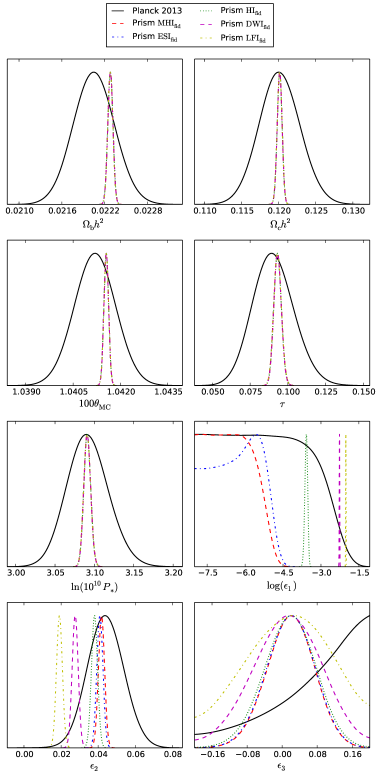
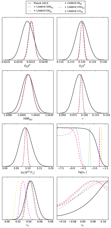
We start this section by presenting the one-dimensional marginalized distributions of the $\Lambda$CDM and inflationary parameters for PRISM and LiteBIRD+Planck in Fig. 1. Concerning the post-inflationary parameters, and $P_{*}$, the corresponding posteriors are strongly peaked at their fiducial values and this is compatible with previous results for PRISM [8]. For LiteBIRD+Planck, it is instructive to compare these posteriors to the ones of Planck 2013 alone (also represented in Fig. 1) as any improvement necessarily comes for LiteBIRD alone.

More interestingly, we notice that for all the fiducial models considered, the posteriors for the cosmological parameters remain the same showing that they do not correlate significantly with the primordial parameters.

Regarding the slow-roll parameters, $\epsilon_{1}$ is, as expected, well determined for $\mathrm{LFI}_{\mathrm{fid}}$, $\mathrm{DWI}_{\mathrm{fid}}$ and $\mathrm{HI}_{\mathrm{fid}}$. For $\mathrm{ESI}_{\mathrm{fid}}$ and $\mathrm{MHI}_{\mathrm{fid}}$, the amount of primordial tensor mode is under the detection threshold and only an upper bound on $\epsilon_{1}$ can be extracted. Let us remark the small bump for $\mathrm{ESI}_{\mathrm{fid}}$ which is at $\epsilon_{1}\simeq 3\times 10^{-6}$ while the underlying fiducial value is $\epsilon_{1}\equiv 3.28\times 10^{-6}$. The second slow-roll parameter $\epsilon_{2}$ is also well inferred and always peaked at its fiducial value which is not surprising as it encodes the tilt of the scalar power spectrum. One remarks that the PRISM precision on this parameter is much better than the LiteBIRD+Planck one.

The situation concerning the third slow-roll parameter $\epsilon_{3}$, which appears at second order in slow roll and determines the running of the power spectra, is completely new [38]. We see that PRISM would be able to constrain this parameter thereby adding a new observable for the inflationary dynamics. This is not the case for LiteBIRD+Planck and can be traced to the range of angular scales accessible to PRISM due to both its resolution and sensitivity.

Figure 2: PRISM two-dimensional marginalized posterior distributions of the slow-roll parameters ($P_{*}$, $\epsilon_{1}$, $\epsilon_{2}$, $\epsilon_{3}$) for the five fiducial models considered, compared to the Planck 2013 two-dimensional posterior distributions (black shaded region). The $\mathrm{MHI}_{\mathrm{fid}}$ red shaded region is almost entirely behind the $\mathrm{ESI}_{\mathrm{fid}}$ blue shaded region.

Figure 3: LiteBIRD+Planck two-dimensional marginalized posterior distributions of the slow-roll parameters ($P_{*}$, $\epsilon_{1}$, $\epsilon_{2}$, $\epsilon_{3}$) for the five fiducial models considered, compared to the Planck 2013 two-dimensional posterior distributions (black shaded region). The $\mathrm{MHI}_{\mathrm{fid}}$ red shaded region is almost entirely behind the $\mathrm{ESI}_{\mathrm{fid}}$ blue shaded region.

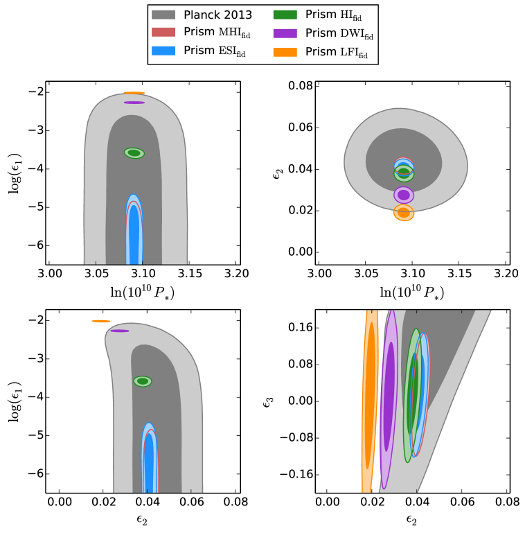
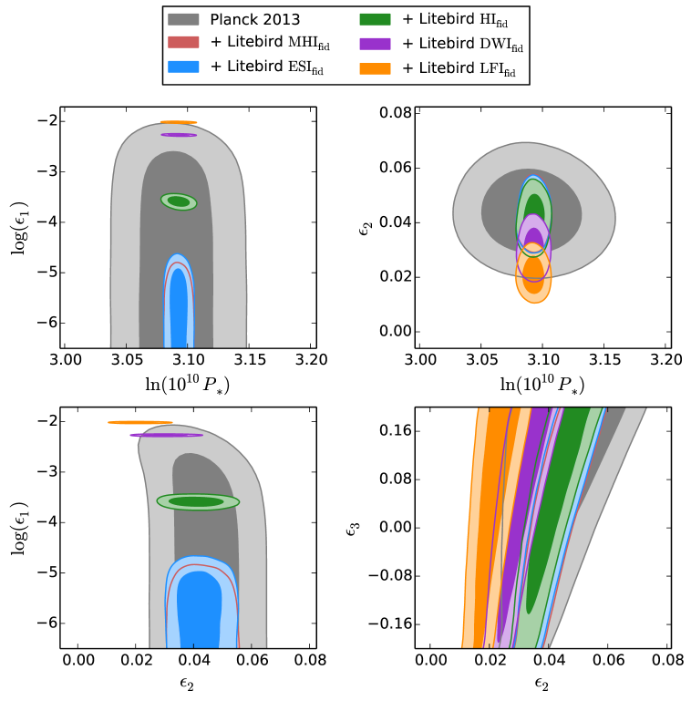
In Figs. 2 and 3, we present the two-dimensional marginalized probability distributions for the primordial parameters $P_{*}$, $\epsilon_{1}$, $\epsilon_{2}$, and $\epsilon_{3}$. The two-dimensional posteriors in the plane $\left(\log\epsilon_{1},\epsilon_{2}\right)$ illustrate the differences in design between PRISM and LiteBIRD. The sensitivity of both experiments in the $B$-modes gives very strong constraints on $\epsilon_{1}$ when the fiducial model lies above the detection threshold. However, as opposed to PRISM, the low angular resolution of LiteBIRD does not allow to significantly improve the determination of $\epsilon_{2}$ compared to Planck alone. Finally, let us again notice that PRISM yields closed contours for the two-sigma confidence intervals in the plane $(\epsilon_{2},\epsilon_{3})$.

Figure 4: PRISM (left) and LiteBIRD+Planck (right) one-dimensional marginalized posterior distributions of the scalar spectral index $n_{\scriptscriptstyle{\mathrm{S}}}$ (top panels) and of the tensor-to-scalar ratio $r$ (bottom panels) for the same five fiducial models compared to the Planck posterior distributions (solid black line). They have been obtained from importance sampling based on the slow-roll parameter posteriors (see Figs. 2 and 3).

Figure 5: PRISM (left) and LiteBIRD (right) two-dimensional marginalized posterior distributions of the derived power law parameters $(n_{\scriptscriptstyle{\mathrm{S}}},r)$ for the five fiducial models under scrutiny compared to the Planck two-dimensional posterior distributions (black shaded region). The $\mathrm{MHI}_{\mathrm{fid}}$ red shaded region is almost entirely hidden behind the one of $\mathrm{ESI}_{\mathrm{fid}}$.

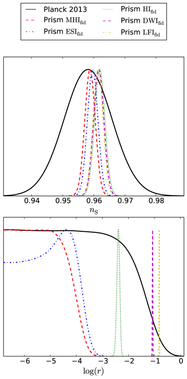
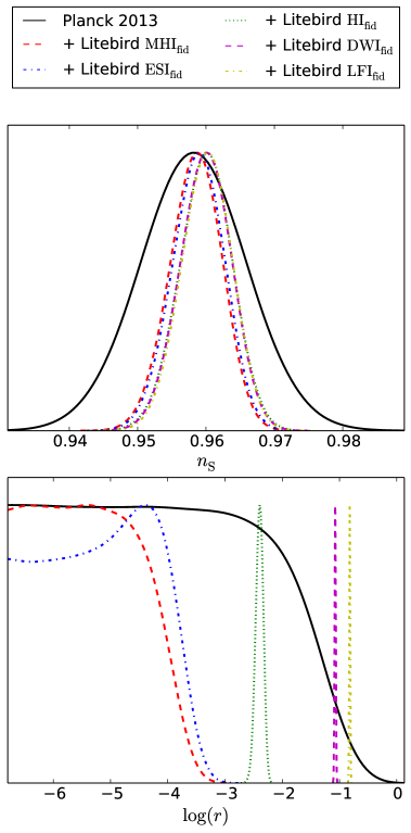
By importance sampling, one can also infer the so-called power-law parameters. In particular, the scalar spectral index $n_{\scriptscriptstyle{\mathrm{S}}}$ and the tensor-to-scalar ratio $r$ are analytic functions of the slow-roll parameters. At second order in slow roll, $n_{\scriptscriptstyle{\mathrm{S}}}$ is given by $n_{\scriptscriptstyle{\mathrm{S}}}=1-2\epsilon_{1}-\epsilon_{2}-2\epsilon_{1}^{2}-(2C+3)\epsilon_{1}\epsilon_{2}-C\epsilon_{2}\epsilon_{3}$ and $r=16\epsilon_{1}+16C\epsilon_{1}\epsilon_{2}$ (the parameter $C\simeq-0.73$ is a numerical constant). The corresponding one-dimensional marginalized distributions for $n_{\scriptscriptstyle{\mathrm{S}}}$ and $r$ are represented in Fig. 4 for PRISM and LiteBIRD+Planck. One notices that, for the five fiducial models, the scalar spectral index is well reconstructed and that its posterior distribution peaks at its fiducial value. For $\mathrm{LFI}_{\mathrm{fid}}$, $\mathrm{DWI}_{\mathrm{fid}}$ and $\mathrm{HI}_{\mathrm{fid}}$, this is because the posterior distributions of $\epsilon_{1}$ and $\epsilon_{2}$ are also well constrained. For $\mathrm{ESI}_{\mathrm{fid}}$ and $\mathrm{MHI}_{\mathrm{fid}}$, there is only an upper bound on $\epsilon_{1}$ but, since it is a very small parameter compared to $\epsilon_{2}$, one has in fact $n_{\scriptscriptstyle{\mathrm{S}}}\simeq 1-\epsilon_{2}$. Therefore, up to the second order corrections, the posterior of $n_{\scriptscriptstyle{\mathrm{S}}}$ is essentially driven by the one on $\epsilon_{2}$. In particular, the difference between the width of these posteriors also comes from different beam resolution between LiteBIRD and PRISM.

Concerning the posterior of $r$, the discussion is essentially similar to the one about the posterior distribution of $\epsilon_{1}$ (since these two parameters are proportional at leading order in slow roll). The quantity $r$ is strongly peaked at its fiducial value for $\mathrm{LFI}_{\mathrm{fid}}$, $\mathrm{DWI}_{\mathrm{fid}}$ and $\mathrm{HI}_{\mathrm{fid}}$, while it is only constrained from above for $\mathrm{ESI}_{\mathrm{fid}}$ and $\mathrm{MHI}_{\mathrm{fid}}$.

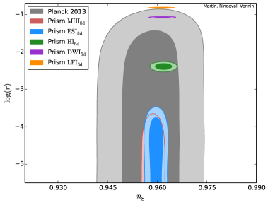
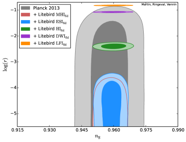
Finally, in Fig. 5, we have represented the two-dimensional posterior distribution in the plane $(n_{\scriptscriptstyle{\mathrm{S}}},\log r)$ for the five different cases studied in this paper.

Figure 6: Distribution of the Encyclopædia Inflationaris models within each Jeffreys’ categories for PRISM and LiteBIRD+Planck and for the five different fiducial models. The Planck [13] and BICEP2 [21] results have been reported for the sake of comparison.

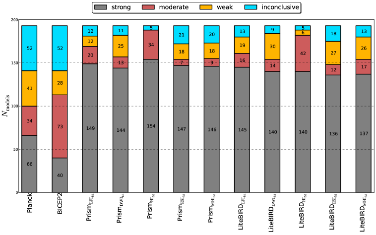
Let us now turn to the computation of the Bayesian evidences. In Fig. 6, for both PRISM and LiteBIRD as well as for each fiducial models ($\mathrm{LFI}_{\mathrm{fid}}$, $\mathrm{DWI}_{\mathrm{fid}}$, $\mathrm{HI}_{\mathrm{fid}}$, $\mathrm{ESI}_{\mathrm{fid}}$ and $\mathrm{MHI}_{\mathrm{fid}}$), we have reported the number of Encyclopædia Inflationaris models in each of the four Jeffreys’ categories giving the strength of belief that the model is explaining the data compared to the best. We have also reported the results obtained in Ref. [13] for Planck 2013 and in Ref. [21] for BICEP2.

One notices the remarkable constraining power of these two experiments: PRISM is able to rule out (“strong” in the Jeffreys’ scale) more than three quarters of the inflationary models in all the situations we have studied, $77\%$ if $\mathrm{LFI}_{\mathrm{fid}}$ is the fiducial model, $75\%$ for $\mathrm{DWI}_{\mathrm{fid}}$, $80\%$ for $\mathrm{HI}_{\mathrm{fid}}$, $76\%$ for $\mathrm{ESI}_{\mathrm{fid}}$ and $76\%$ for $\mathrm{MHI}_{\mathrm{fid}}$. These numbers are similar (although slightly smaller) for LiteBIRD+Planck, namely $75\%$ for $\mathrm{LFI}_{\mathrm{fid}}$, $73\%$ for $\mathrm{DWI}_{\mathrm{fid}}$, $73\%$ for $\mathrm{HI}_{\mathrm{fid}}$, $70\%$ for $\mathrm{ESI}_{\mathrm{fid}}$ and $71\%$ for $\mathrm{MHI}_{\mathrm{fid}}$. One should compare these performances to the Planck (and BICEP2) results that are able to respectively reject $34\%$ and $21\%$ of the inflationary scenarios. It is also interesting to remark that the percentage of models in the strong zone does not depend a lot on the assumed fiducial model and, therefore, appears to be quite generic.

Let us now discuss the opposite end of the Jeffreys’ scale, namely the models in the “inconclusive” zone.

For PRISM with $\mathrm{LFI}_{\mathrm{fid}}$ as fiducial model, we find that only $6\%$ of the scenarios are in this category. If, in addition, we take into account the Bayesian complexity and restrict ourselves to models having a number of unconstrained parameter between zero and one, then this number falls to $4\%$.

In the case of the fiducial model $\mathrm{DWI}_{\mathrm{fid}}$, one finds very similar numbers. For PRISM, we get $6\%$ in the “inconclusive” zone and $3\%$ in the “inconclusive” zone having a number of unconstrained parameters between zero and one.

If the fiducial model is now the Starobinsky model, $\mathrm{HI}_{\mathrm{fid}}$, then the performances are even better: only $3\%$ of the models are in the inconclusive zone and, if one considers only the scenarios with a number of unconstrained parameters between zero and one, then one singles out a subset of three models only, corresponding to $1.5\%$ of the total number of Encyclopædia Inflationaris scenarios. It appears that if the inflationary model actually realized in Nature is similar to $\mathrm{HI}_{\mathrm{fid}}$, then PRISM and LiteBIRD+Planck would provide an optimal setting.

In the case where $\mathrm{ESI}_{\mathrm{fid}}$ is the fiducial model, $11\%$ of the scenarios are in the inconclusive zone (and $4\%$ if the number of unconstrained parameters is taken between zero and one). Let us recall that, in this situation, and contrary to the three preceding examples, the detection of primordial gravity waves is no longer possible.

Finally, the case where $\mathrm{MHI}_{\mathrm{fid}}$ is the fiducial scenario is quite similar. As for $\mathrm{ESI}_{\mathrm{fid}}$, this corresponds to a situation where the tensor-to-scalar ratio $r$ is too small to be measured, even by the PRISM experiment. One finds $11\%$ in the inconclusive category and $4\%$ if Bayesian complexity is also taken into account.

For LiteBIRD+Planck, these figures are almost the same while being in a non-significant way slightly less constraining (see Fig. 6). Only for $\mathrm{ESI}_{\mathrm{fid}}$ and $\mathrm{MHI}_{\mathrm{fid}}$, one finds less models in the inconclusive zone ($9\%$ and $7\%$, respectively), but this is due to a boundary effect as there are more models in the weak evidence zone.

In view of these results, a word of caution is in order. Indeed, one might naively conclude that a simple design like LiteBIRD, combined with Planck, would perform as well as a big mission like PRISM. However, here, we have assumed perfect foregrounds removal for both LiteBIRD and PRISM. This may be justified for PRISM because the mission is precisely designed to accurately measure various other astrophysical signals (such as the Cosmic Infrared Background, etc…) in addition to the CMB thereby allowing an optimal components separation [8]. This might not be the case for LiteBIRD and our forecasts for LiteBIRD+Planck may be over-idealized. Moreover, as it should be clear from Fig. 1, only PRISM will have the ability to measure $\epsilon_{3}$, that is to say the slow-roll running of the scalar power spectrum [38]. This is not so relevant for the model comparison here, precisely because all slow-roll models necessarily produce small values of $\epsilon_{3}$. However, if slow-roll ends up being violated at second order ($\epsilon_{3}>1$), PRISM will have the ability to detect it.

4 Conclusions

Let us now summarize our main findings. In this paper, we have studied the ability to constrain the inflationary theory of two post-Planck CMB missions: PRISM and LiteBIRD. Our method consists in simulating CMB data for five different inflationary scenarios corresponding to a representative sample of inflationary models, leading to different values of the tensor-to-scalar ratio $r$ smaller and larger that the target of those mission $r\simeq 10^{-3}$. For each mock data, we have computed the Bayesian evidences and complexities of all Encyclopædia Inflationaris models and have studied how they are distributed among the four Jeffreys’ categories with respect to the best model. We have found that the number of models that can be ruled out at a statistically significant level typically goes from one third for Planck to three quarters for PRISM and LiteBIRD+Planck. The gain in constraining power is therefore significant, illustrating the efficiency of constraining the observable $r$ (or $\epsilon_{1}$) as well as improving the measurement accuracy on the other primordial parameters.

Let us stress again that our results have been derived in what we have called “the worst case scenario”, namely for single-field slow-roll models. Indeed, these are considered to be the most difficult to infer as they produce an undetectable amount of non-Gaussianities and do not generate entropy perturbations. In a wider framework in which one would consider non-minimal inflationary models, one could only expect stronger constraints (see for instance Refs. [8, 39]). In this context, we have found that PRISM could rule out slow-roll inflation by its ability to measure a less than unity second order slow-roll parameter $\epsilon_{3}$, a result which has been discussed before only in the context of future 21cm experiments [40, 41].

Finally, let us discuss possible improvements of the present work. Going further than estimating the constraining power of the future CMB missions, it would be interesting to investigate the model identification problem. For instance, for the PRISM mission, we have checked that the Bayesian evidence of $\mathrm{DWI}_{25}$, a model sharing exactly the same potential shape as $\mathrm{DWI}_{\mathrm{fid}}$ but having an unknown reheating temperature and unknown potential normalization ($P_{*}$) would end up being moderately disfavored compared to $\mathrm{DWI}_{\mathrm{fid}}$. Another model $\mathrm{DWI}_{25}^{\mathrm{reh}}$, taken to be of same potential shape and reheating temperature than $\mathrm{DWI}_{\mathrm{fid}}$, but still having an unknown potential normalization, would remain within the inconclusive region compared to $\mathrm{DWI}_{\mathrm{fid}}$. This suggests that identifying the “correct” inflationary scenario with a mission like PRISM will necessitate to have a good prior knowledge on the reheating energy scale. Conversely, this also suggests that blindly looking at the potential shape without specifying how the reheating proceeds could lead to false positive identifications of the inflationary model. In other words, these future CMB missions will reach an accuracy such that specifying couplings of the inflaton to the Standard Model of particle physics will become compulsory [42] and will actually be seen in the CMB sky [38].

References

- [1] BICEP2 Collaboration Collaboration, P. Ade et al., Detection of B-Mode Polarization at Degree Angular Scales by BICEP2, Phys.Rev.Lett. 112 (2014) 241101, [arXiv:1403.3985].
- [2] BICEP2 Collaboration Collaboration, P. Ade et al., BICEP2 II: Experiment and Three-Year Data Set, Astrophys.J. 792 (2014) 62, [arXiv:1403.4302].
- [3] R. Flauger, J. C. Hill, and D. N. Spergel, Toward an Understanding of Foreground Emission in the BICEP2 Region, JCAP 1408 (2014) 039, [arXiv:1405.7351].
- [4] M. J. Mortonson and U. Seljak, A joint analysis of Planck and BICEP2 B modes including dust polarization uncertainty, JCAP 1410 (2014), no. 10 035, [arXiv:1405.5857].
- [5] Planck Collaboration Collaboration, P. Ade et al., Planck intermediate results. XIX. An overview of the polarized thermal emission from Galactic dust, arXiv:1405.0871.
- [6] J. Bock, A. Cooray, S. Hanany, B. Keating, A. Lee, et al., The Experimental Probe of Inflationary Cosmology (EPIC): A Mission Concept Study for NASA’s Einstein Inflation Probe, arXiv:0805.4207.
- [7] T. Matsumura, Y. Akiba, J. Borrill, Y. Chinone, M. Dobbs, et al., Mission design of LiteBIRD, arXiv:1311.2847.
- [8] PRISM Collaboration Collaboration, P. André et al., PRISM (Polarized Radiation Imaging and Spectroscopy Mission): An Extended White Paper, JCAP 1402 (2014) 006, [arXiv:1310.1554].
- [9] COrE, “A satellite mission for probing cosmic origins, neutrinos masses and the origin of stars and magnetic fields.” http://www.core-mission.org/science.php.
- [10] K. Sigurdson and A. Cooray, Cosmic 21-cm delensing of microwave background polarization and the minimum detectable energy scale of inflation, Phys.Rev.Lett. 95 (2005) 211303, [astro-ph/0502549].
- [11] T. Namikawa and R. Nagata, Lensing reconstruction from a patchwork of polarization maps, JCAP 1409 (2014) 009, [arXiv:1405.6568].
- [12] Planck Collaboration Collaboration, P. Ade et al., Planck 2013 results. XXII. Constraints on inflation, arXiv:1303.5082.
- [13] J. Martin, C. Ringeval, R. Trotta, and V. Vennin, The Best Inflationary Models After Planck, JCAP 1403 (2014) 039, [arXiv:1312.3529].
- [14] X. Chen and C. Ringeval, Searching for Standard Clocks in the Primordial Universe, JCAP 1208 (2012) 014, [arXiv:1205.6085].
- [15] R. Trotta, Applications of Bayesian model selection to cosmological parameters, Mon.Not.Roy.Astron.Soc. 378 (2007) 72–82, [astro-ph/0504022].
- [16] R. Trotta, Bayes in the sky: Bayesian inference and model selection in cosmology, Contemp.Phys. 49 (2008) 71–104, [arXiv:0803.4089].
- [17] J. Martin, C. Ringeval, and R. Trotta, Hunting Down the Best Model of Inflation with Bayesian Evidence, Phys.Rev. D83 (2011) 063524, [arXiv:1009.4157].
- [18] R. Easther and H. V. Peiris, Bayesian Analysis of Inflation II: Model Selection and Constraints on Reheating, Phys.Rev. D85 (2012) 103533, [arXiv:1112.0326].
- [19] J. Martin, C. Ringeval, and V. Vennin, Encyclopædia Inflationaris, Phys.Dark Univ. (2014) [arXiv:1303.3787].
- [20] J. Martin, Inflation after Planck: and the winners are, arXiv:1312.3720.
- [21] J. Martin, C. Ringeval, R. Trotta, and V. Vennin, Compatibility of Planck and BICEP2 in the Light of Inflation, Phys.Rev. D90 (Sept., 2014) 063501, [arXiv:1405.7272].
- [22] M. Kunz, R. Trotta, and D. Parkinson, Measuring the effective complexity of cosmological models, Phys.Rev. D74 (2006) 023503, [astro-ph/0602378].
- [23] C. Ringeval, Fast Bayesian inference for slow-roll inflation, Mon.Not.Roy.Astron.Soc. 439 (2014) 3253, [arXiv:1312.2347].
- [24] J. Martin and C. Ringeval, First CMB Constraints on the Inflationary Reheating Temperature, Phys.Rev. D82 (2010) 023511, [arXiv:1004.5525].
- [25] L. Dai, M. Kamionkowski, and J. Wang, Reheating constraints to inflationary models, Phys.Rev.Lett. 113 (2014) 041302, [arXiv:1404.6704].
- [26] M. B. Hoffman and M. S. Turner, Kinematic constraints to the key inflationary observables, Phys.Rev. D64 (2001) 023506, [astro-ph/0006321].
- [27] D. J. Schwarz, C. A. Terrero-Escalante, and A. A. Garcia, Higher order corrections to primordial spectra from cosmological inflation, Phys.Lett. B517 (2001) 243–249, [astro-ph/0106020].
- [28] J. Martin, C. Ringeval, and V. Vennin, K-inflationary Power Spectra at Second Order, JCAP 1306 (2013) 021, [arXiv:1303.2120].
- [29] J. Beltran Jimenez, M. Musso, and C. Ringeval, Exact Mapping between Tensor and Most General Scalar Power Spectra, Phys.Rev. D88 (2013) 043524, [arXiv:1303.2788].
- [30] A. Lewis, A. Challinor, and A. Lasenby, Efficient computation of CMB anisotropies in closed FRW models, Astrophys.J. 538 (2000) 473–476, [astro-ph/9911177].
- [31] J. Bond, A. H. Jaffe, and L. Knox, Radical compression of cosmic microwave background data, Astrophys.J. 533 (2000) 19, [astro-ph/9808264].
- [32] L. Perotto, J. Lesgourgues, S. Hannestad, H. Tu, and Y. Y. Wong, Probing cosmological parameters with the CMB: Forecasts from full Monte Carlo simulations, JCAP 0610 (2006) 013, [astro-ph/0606227].
- [33] W. J. Percival and M. L. Brown, Likelihood methods for the combined analysis of CMB temperature and polarisation power spectra, Mon.Not.Roy.Astron.Soc. 372 (2006) 1104–1116, [astro-ph/0604547].
- [34] S. Hamimeche and A. Lewis, Likelihood Analysis of CMB Temperature and Polarization Power Spectra, Phys.Rev. D77 (2008) 103013, [arXiv:0801.0554].
- [35] P. Mukherjee, D. Parkinson, and A. R. Liddle, A Nested Sampling Algorithm for Cosmological Model Selection, Astrophys. J. 638 (2006) L51–L54, [astro-ph/0508461].
- [36] F. Feroz and M. Hobson, Multimodal nested sampling: an efficient and robust alternative to MCMC methods for astronomical data analysis, Mon.Not.Roy.Astron.Soc. 384 (2008) 449, [arXiv:0704.3704].
- [37] F. Feroz, M. Hobson, and M. Bridges, MultiNest: an efficient and robust Bayesian inference tool for cosmology and particle physics, Mon.Not.Roy.Astron.Soc. 398 (2009) 1601–1614, [arXiv:0809.3437].
- [38] J. Martin, C. Ringeval, R. Trotta, and V. Vennin in preparation, 2014.
- [39] S. Clesse, B. Garbrecht, and Y. Zhu, Testing Inflation and Curvaton Scenarios with CMB Distortions, JCAP 1410 (2014), no. 10 046, [arXiv:1402.2257].
- [40] P. Adshead, R. Easther, J. Pritchard, and A. Loeb, Inflation and the Scale Dependent Spectral Index: Prospects and Strategies, JCAP 1102 (2011) 021, [arXiv:1007.3748].
- [41] S. Clesse, L. Lopez-Honorez, C. Ringeval, H. Tashiro, and M. H. Tytgat, Background reionization history from omniscopes, Phys.Rev. D86 (2012) 123506, [arXiv:1208.4277].
- [42] J. Garcia-Bellido, D. G. Figueroa, and J. Rubio, Preheating in the Standard Model with the Higgs-Inflaton coupled to gravity, Phys.Rev. D79 (2009) 063531, [arXiv:0812.4624].
- [43] A. Lewis and S. Bridle, Cosmological parameters from CMB and other data: A Monte Carlo approach, Phys.Rev. D66 (2002) 103511, [astro-ph/0205436].