11email: daniel.michalik@astro.lu.se, lennart@astro.lu.se, david@astro.lu.se 22institutetext: European Space Agency (ESA/ESAC), P.O. Box 78, ES-28691 Villanueva de la Cañada, Madrid, Spain
22email: uwe.lammers@sciops.esa.int
Joint astrometric solution of Hipparcos and Gaia
Abstract
Context. The first release of astrometric data from Gaia is expected in 2016. It will contain the mean stellar positions and magnitudes from the first year of observations. For more than 100 000 stars in common with the Hipparcos Catalogue it will be possible to compute very accurate proper motions due to the time difference of about 24 years between the two missions. This Hundred Thousand Proper Motions (htpm) project is planned to be part of the first release.
Aims. Our aim is to investigate how early Gaia data can be optimally combined with information from the Hipparcos Catalogue in order to provide the most accurate and reliable results for htpm.
Methods. The Astrometric Global Iterative Solution (agis) was developed to compute the astrometric core solution based on the Gaia observations and will be used for all releases of astrometric data from Gaia. We adapt agis to process Hipparcos data in addition to Gaia observations, and use simulations to verify and study the joint solution method.
Results. For the htpm stars we predict proper motion accuracies between 14 and 134 as yr-1, depending on stellar magnitude and amount of Gaia data available. Perspective effects will be important for a significant number of htpm stars, and in order to treat these effects accurately we introduce a formalism called smok (scaled model of kinematics). We define a goodness-of-fit statistic which is sensitive to deviations from uniform space motion, caused for example by binaries with periods of 10–50 years.
Conclusions. htpm will significantly improve the proper motions of the Hipparcos Catalogue well before highly accurate Gaia-only results become available. Also, htpm will allow us to detect long period binary and exoplanetary candidates which would be impossible to detect from Gaia data alone. The full sensitivity will not be reached with the first Gaia release but with subsequent data releases. Therefore htpm should be repeated when more Gaia data become available.
Key Words.:
Astrometry – Methods: data analysis – Methods: numerical – Space vehicles: instruments – Proper motions – Planets and satellites: detection1 Introduction
Stellar proper motions have traditionally been determined by analysing the differences in position at different epochs, often separated by many decades and obtained using vastly different instruments and methods. In this process, parallaxes (and radial motions, albeit relevant to a much lesser extent) were mostly ignored.
With the advent of space astrometry, most notably the European satellite Hipparcos (1989–1993, see ESA 1997), it became necessary to treat data in a unified manner, i.e., by applying a single least-squares solution for the position, parallax, and annual proper motion. Hipparcos determined these parameters for nearly stars111We use “star” to denote a catalogue entry even when it refers to a non-single or extragalactic object. In the context of Gaia data processing the term “source” is commonly used for such objects. mostly brighter than magnitude , with a median uncertainty of about 1 milli-arcsecond (mas). The Tycho-2 Catalogue (Høg et al. 2000) gave additional data for 2.5 million stars observed with the Hipparcos starmappers. The re-reduction of the Hipparcos raw data (van Leeuwen 2007a, b) significantly improved the main-mission results. Today, 25 years after the launch of the satellite, these catalogues remain the main source for the astrometric parameters of these stars.
The European space astrometry mission Gaia will soon change this picture. Gaia, launched at the end of 2013, will determine the astrometric parameters of up to a billion stars between magnitude and with unprecedented accuracies reaching a few tens of micro-arcseconds (as) for Gaia magnitude . The vast amounts of data will be processed in a single coherent least-squares solution, which solves not only for the astrometric parameters but also for a large number of parameters describing the time-varying spacecraft attitude and the geometry of the optical instrument. Due to the very large number of parameters to be determined from the observational data the system cannot be solved directly (Bombrun et al. 2010) but has to be tackled in a block-iterative manner with the so called “Astrometric Global Iterative Solution” (agis). The agis software has been designed and implemented by groups at ESA/ESAC, Lund Observatory and others, and is described in detail together with the fundamental algorithms and mathematical framework by Lindegren et al. (2012).
Astrometric measurements obtained in the past, even of moderate accuracy by modern standards, have lasting value as they represent a state of the Universe that is never repeated. A good example is the construction of proper motions in the Tycho-2 Catalogue using Hipparcos and century-old photographic positions. When the astrometric parameters are propagated over a long time interval, uncertainties in the tangential and radial motions accumulate to a significant positional uncertainty. Yet long-term deviations from linear space motion (e.g., in long-period binaries) increase even more drastically with time. Such deviations might not be detectable within the time spans of the Hipparcos or Gaia missions individually, but could be detectable by combining the results of the two. Thus, although Hipparcos will soon be superseded by Gaia in terms of the expected accuracies at current epochs, its data form a unique comparison point in the past, very valuable in combination with later results. For this reason the first Gaia data release scheduled for 2016 will not only publish stellar positions and magnitudes based on the first Gaia observations, but also a combination of these observations with the Hipparcos Catalogue for all stars common between the two missions. This part of the release is called the Hundred Thousand Proper Motions project (htpm), originally proposed by F. Mignard in a Gaia-internal technical document (Mignard 2009).
This paper gives a recipe for the practical realisation of the htpm project in the context of the already existing agis scheme for the astrometric solution of Gaia data. The proper motions in htpm might be trivially computed from the positional differences between an early Gaia solution and the Hipparcos Catalogue – the “conventional catalogue combination” approach of Sect. 2.3. However, we argue that the more elaborate “joint solution” method described in Sect. 2.4 will have important advantages for the htpm project, and in Sect. 3 we show how to implement it as part of agis. The validity and accuracy of the method is demonstrated by means of a joint solution of simulated Gaia observations of the Hipparcos stars (Sect. 4). In the final sections we discuss the limitations of the results and their validity in the light of Gaia’s full nominal mission performance, as well as possible applications of the joint solution method to other astrometric data.
The htpm project should use the re-reduction of the raw Hipparcos data (van Leeuwen 2007b), as it represents a significant improvement over the original Hipparcos Catalogue (ESA 1997). Therefore it is also used in all our simulations. For the purpose of demonstrating the htpm solution we regard all valid entries of the Hipparcos Catalogue as astrometrically well-behaved (effectively single) stars. Their space motions are therefore regarded as uniform (rectilinear, with constant speed) over the time interval covered by Hipparcos and Gaia. This is obviously a very simplified picture of the true content of the Hipparcos Catalogue. However, getting the solution right in this simple case is a first necessary step for any more sophisticated treatment of detected binaries and multiple stars in the Hipparcos Catalogue.
2 Theory
Combining astrometric catalogues requires that data are expressed in the same reference system and described in terms of a common kinematic model. In this section we describe the adopted model and how it is connected to the definition of the astrometric parameters. We outline the conventional approach to catalogue combination and develop the “joint solution” as an optimal generalisation of the method. We show how to detect deviations from the kinematic model or misfits between the datasets. We also outline how to reconstruct the required information from Hipparcos and how to integrate the proposed scheme in the astrometric solution algorithm of Gaia.
2.1 Kinematic model of stellar motion
The choice of astrometric parameters is a direct result of choosing a model of stellar motion. The most basic assumption is for stars to move uniformly, i.e., linearly and with constant speed, relative to the Solar System Barycentre (SSB). Note that this also means that the stars are assumed to be single. This is obviously not true for all of them, but a good basic assumption for most stars. During the data reduction stars that are not “well behaved” in an astrometric sense can be filtered out and treated further, e.g., by adding additional parameters for components of stellar systems or for acceleration through external influences.
A uniform space motion can be fully described by six parameters: three for the position in space at a chosen reference epoch, and three for the velocity. Traditionally, the three positional parameters are right ascension , declination , and parallax relative to the SSB at the reference epoch of the catalogue. The motion is then described by three parameters, where and are the proper motions in right ascension and declination, respectively, and the third parameter is the radial motion component. The radial component is more commonly given as the radial velocity in km s-1, but in an astrometric context it is conveniently expressed as the radial proper motion (equivalent to the relative change in distance over time, or )
| (1) |
where is the astronomical unit expressed in km yr s-1. Only the first five parameters are classically considered astrometric parameters. Based on only a few years of observations it is usually not possible to determine the radial component from astrometry with sufficient accuracy (Dravins et al. 1999). Hence the radial component is better determined by other techniques, i.e., from spectroscopy. For Gaia the radial component will be significant for many more stars, although the affected fraction remains very small (de Bruijne & Eilers 2012). Even though is not determined in the astrometric solution for the vast majority of sources, it is convenient and sometimes necessary to formulate astrometric problems with the full set of six astrometric parameters, as we do in this paper. We will also show how to treat the sixth component when the radial velocity is unknown or added from spectroscopy.
2.2 Dealing with non-linearities: smok
When comparing and subsequently combining astrometric catalogues one needs to deal with the fact that the mapping from rectilinear to spherical coordinates is strongly non-linear. This becomes significant at the as level when the differences in and exceed some arcsec. For example, the barycentric direction traced out in , due to the proper motion will not be linear even though the star is assumed to move uniformly through space. The traditional way to deal with this is to introduce higher-order correction terms computed by Taylor expansion of the rigorous equations (e.g., Taff 1981). In this paper we take a different approach, based on the “scaled modelling of kinematics” (smok) concept described in Appendix A. For the present purpose it is sufficient to know that may be replaced by linear coordinates relative to a designated, fixed comparison point, with time derivatives , representing the components of proper motion in and . The six parameters , , , , , (where is the smok equivalent of the radial proper motion) provide an alternative and equivalent parametrization of the kinematics, more convenient for the catalogue combination than the usual set , , , , , .
2.3 Conventional catalogue combination
In the conventional catalogue combination the astrometric parameters in each catalogue are independently estimated from separate sets of observations, and the combination is done a posteriori from the individual catalogues. Let () at time be the position and parallax of a star in the first catalogue, and () at time the corresponding information in the second catalogue. The proper motion parameters , are then derived as the positional difference over time
| (2) |
which is possible thanks to the reformulation of the astrometric parameters in smok. The proper motion uncertainties are
| (3) |
where is the uncertainty of , etc. The third kinematic parameter for the radial motion could in theory be derived from the (negative, relative) difference in parallax, but in practice it is derived from the spectroscopic radial velocity as discussed in Sect. 2.1.
While the proper motions are obtained by taking position differences over time, the combined parameters for position and parallax are formed as weighted means. For this gives
| (4) |
referring to the mean epoch of the combination
| (5) |
The reference time is the optimal time in-between the two catalogues at which the position and proper motion are uncorrelated and the uncertainty of is minimal, given by . The expressions for and are analogous.
This combination scheme has some limitations, in that it does not take correlations between the astrometric parameters into account, nor the individual proper motions that may exist in each catalogue. In the next section we describe a more general approach.
2.4 Joint solution
The reduction of astrometric data is typically done using least-squares solutions, resulting in a linear system of normal equations . Here, is the vector of resulting astrometric parameters, the normal equations matrix, and a vector constructed from the residuals of the problem.222The least squares problem can be solved using a number of alternative numerical algorithms, for example based on orthogonal transformations. However, as these algorithms are all mathematically equivalent to the use of normal equations, our results remain valid independent of the chosen solution algorithm. The covariance of the solution is formally given by .
In agis the observations of all well-behaved stars (“primary sources”) must be considered together in a single, very large least-squares solution (Sect. 2.7). For primary sources, would then be the full vector of astrometric parameters, with and of corresponding dimensions. However, for the present exposition it is sufficient to consider one star at a time, so that and are of length 6 and has dimensions . In practice only five of the six parameters are estimated, and should hereafter be regarded as the inverse of the upper-left submatrix.333The full matrix is nevertheless needed for the covariance propagation in Sect. 2.6.
On the assumption that the adopted kinematic model is valid for a particular star, the matrix and vector encapsulate the essential information on the astrometric parameters, as determined by the least-squares solution. Thus, in order to make optimal use of the Hipparcos data for a given star there is no need to consider the individual observations of that star: all we need is contained in the “information array” . In Sect. 2.6 we show how this array is reconstructed from the published Hipparcos Catalogue.
Let and be the information arrays for the same star as given by two independent astrometric catalogues. From the way the normal equations are calculated from observational data it is clear that the information arrays are additive, so that is the information array that would have resulted from processing the two datasets together. In Michalik et al. (2012) we have proposed that the optimum combination of the catalogues is done a priori, that is by adding the corresponding arrays before solving. The result,
| (6) |
is the joint solution of the astrometric parameters, with covariance . The two catalogue entries for the star must use the same reference epoch and the same smok comparison point.
The joint solution has several advantages over the conventional combination method outlined in Sect. 2.3. Because it uses the full information in each catalogue it makes better use of the data and allows to estimate the resulting uncertainties more accurately, taking into account the correlations. The individual proper motion information available in each catalogue is automatically incorporated in the joint proper motion. Moreover, a solution might be possible where the data in each set individually is insufficient to solve for all astrometric parameters, that is, may be non-singular even if , , or both, are singular. In practice if comes from the Hipparcos data it will always be non-singular (since there is a Hipparcos solution), and the sum is then also non-singular. Hence it will always be possible to make a joint solution for all five astrometric parameters of the htpm stars, Finally, the joint solution scheme is a clean and rigorous approach and can be integrated into the existing implementation of the astrometric solution for Gaia with moderate effort.
The joint solution can be seen as a multidimensional generalisation of the conventional scheme in Sec. 2.3, with representing the weights () and the astrometric parameters multiplied by their weights (e.g., ). Then Eq. (6) is the matrix equivalent of Eq. (4). The joint solution can also be understood in terms of Bayesian estimation theory (assuming multivariate Gaussian parameter errors), with representing the prior information, the new data, and their sums the posterior information.
2.5 Goodness of fit of the joint solution
The goodness of fit of a least-squares solution can be described in terms of the sum of the squares of the normalized post-fit residuals,
| (7) |
where and are the observed and calculated (fitted) angular focal-plane coordinates of the star in observation , and is the standard error of the observation. is calculated for each star separately and is simply a function of . The least-squares solution minimizes and for any other parameter vector we have
| (8) |
If the kinematic model is correct and the standard errors of the observations are correctly estimated one expects the minimum value to follow the chi-square distribution with degrees of freedom, . Here is equal to the number of observations (that is the number of terms in Eq. 7) diminished by the rank of . Note that this holds even if is singular (i.e., , where is the number of fitted parameters). In the singular case is not unique, yet has a well-defined value (which may be 0 or positive).
Analogous to Eq. (8), in the joint solution we minimize the total goodness of fit,
| (9) |
Here is the solution obtained by using only catalogue , i.e., minimizing , which results in the minimum value . It is readily seen that Eq. (9) is minimized precisely for the joint solution vector in Eq. (6).
Each of the four terms in Eq. (9) has a simple interpretation. The first term, , is the chi-square obtained when fitting the astrometric parameters only to the first set of data (in our case the Hipparcos data); similarly, is the chi-square obtained when fitting only to the second set of data (from Gaia). The sum of the last two terms is minimized for , and shows how much the chi-square is increased by forcing the same parameters to fit both sets of data in the joint solution. This quantity is useful for assessing whether the two datasets are mutually consistent and we therefore introduce a separate notation for it,
| (10) |
The two terms give the increase in chi-square due to the first and second dataset, respectively.
Long-period astrometric binaries may have significantly different proper motions at the Hipparcos and Gaia epochs, and these in turn may differ from the mean proper motion between the epochs. If the differences are significant, compared with the measurement precisions, they will result in an increased value of . The null hypothesis, namely that the star is astrometrically well-behaved, should be rejected if exceeds a certain critical value. In order to calculate the critical value it is necessary to know the expected distribution of under the null hypothesis.
Let and be the number of observations and degrees of freedom in catalogue . The number of degrees of freedom in the joint solution is . Under the null-hypothesis we have (, 2), , and consequently
| (11) |
where
| (12) |
In the special case when , , and all have full rank (equal to , the number of astrometric parameters) we have . At a significance level of 1% the critical values of , above which the null hypothesis should be rejected, are 15.086, 13.277, 11.345, 9.210, and 6.635 for , 4, 3, 2, and 1, respectively (e.g., Abramowitz & Stegun 2012). With this criterion only 1% of the well-behaved stars should be accidentally misclassified as not well-behaved. The expected distribution of can be verified in the simulations which, by design, only includes well-behaved stars.
2.6 Reconstruction of , for the Hipparcos Catalogue
When using the joint solution for incorporating Hipparcos data in the solution of early Gaia data it is necessary to reconstruct the normal matrix and the right hand side from Hipparcos for each star. These are initially calculated for the reference epoch of the Hipparcos catalogue (J1991.25) and later propagated to the adopted reference epoch of the joint solution (see Sect. 2.7).
Let , , , , be the astrometric parameters from the Hipparcos Catalogue after transformation into the smok notation (see Appendix A). The upper-left submatrix of the covariance matrix can be taken without changes from the Hipparcos Catalogue (see Appendix B for details) since , , with sufficient accuracy at the reference epoch of the catalogue and provided that the smok comparison point is close enough to the astrometric parameters of the star. The sixth parameter and its corresponding entries in the covariance matrix need to be added from external sources or set to sensible values if not available (see below). Then the normal matrix is simply the inverse of the covariance matrix and
| (13) |
ESA (1997), Volume 1, Eq. [1.5.69] shows how to reconstruct the elements , that is the sixth column and row of the covariance matrix corresponding to the radial motion . Let , , be the true values and , , the errors. The expression in Eq. [1.5.69] for the diagonal element is only valid if the relative uncertainties in the radial velocity and parallax are small, i.e., , . If this is not the case we need to consider the complete expression for the calculated radial motion,
| (14) |
where , leading to
| (15) |
Squaring and taking the expectation while assuming that the errors in parallax and radial velocity are uncorrelated gives
| (16) |
where we replaced the true quantities by the observed ones. The third term is the required generalization if or is zero, or if the relative errors are large. For example, if parallax and radial motion are unknown they could be assumed to be zero with a large uncertainty. The generalized version of Eq. [1.5.69] in ESA (1997) reads
| (17) |
The Hipparcos Catalogue contains numerous entries for non-single stars, for which additional parameters are given, describing deviations from uniform space motion. These additional parameters are ignored in our simulations, which regard every star as single. In the actual htpm solution many of these stars may require more specialised off-line treatment. This is not further discussed in this paper.
2.7 Joint solution in agis
In reality the astrometric solution cannot be done separately for each star as described in Sect. 2.4 but must consider all the stars together with the spacecraft attitude and instrument calibration. Without prior information on the astrometric parameters this leaves the solution undetermined with respect to the reference frame. This is not the case for the joint solution, however, as the Hipparcos prior information contains positions and proper motions that are expressed in a specific reference frame, namely the Hipparcos realisation of the International Celestial Reference System (icrs; Feissel & Mignard 1998). The incorporation of the Hipparcos prior in the joint solution automatically ensures that the resulting data are on the Hipparcos reference frame. If required, the data can later be transformed into a more accurate representation of the ICRS (see Sect. 5.3).
Due to the size of the data reduction problem agis does not directly solve but iteratively improves the astrometric parameters by computing the updates , i.e., the difference to the current best estimate values. When incorporating Hipparcos data this requires us to also express the Hipparcos data (subscript H) as a difference to the current best estimate (subscript c). Therefore we construct
| (18) |
Before solving we add the corresponding matrices for the Gaia data. If no additional Gaia data would be added the solution would immediately recover the Hipparcos Catalogue parameters.
The reference epoch of the joint solution can be arbitrarily chosen. In practice the Gaia data are much better than the Hipparcos data, therefore the optimal reference epoch would always be very close to the epoch of the Gaia data alone. Assuming one releases Gaia-only data and htpm results at the same time it might be convenient to publish both for the same reference epoch, i.e., the Gaia-only reference epoch of the data release.
3 Simulations
3.1 Logic of simulations
Simulations are based on agislab (Holl et al. 2012), a small-scale version of the agis data reduction created and maintained at Lund Observatory. It is used to aid the development of algorithms for the astrometric data reduction of Gaia. Simulation runs are carried out in the following steps (cf. Fig. 1):
-
1.
Creating catalogues of all the stars used in the simulation, namely the Hipparcos stars and the auxiliary stars (see below). Two catalogues are needed: a simulated “true” catalogue to generate Gaia observations and to evaluate the uncertainties of the astrometric performance, and an initial catalogue of starting values for the data reduction;
-
2.
Simulating observations of the stars using the Nominal Scanning Law (de Bruijne et al. 2010), including perturbations according to the expected precision of Gaia measurements;
-
3.
Improving the astrometry of the initial catalogue through the astrometric solution (agis), resulting in the final catalogue. This can be done with or without incorporation of prior information from Hipparcos;
-
4.
Evaluating the error of the resulting solution by comparing the final catalogue with the true catalogue.
Details of the first two steps are given below, while remaining steps are covered in Sect. 4.
3.2 Simulating the stellar catalogues
All catalogues consist of two parts, the Hipparcos stars and the additional auxiliary stars. The Hipparcos stars are necessary for the realisation of the htpm scheme, and 113 396 stars are within the nominal magnitude range of Gaia (–20). In order to obtain a reliable astrometric solution with a realistic modelling of the attitude constraints we find that a minimum of one million stars is needed, uniformly distributed on the sky. 886 604 auxiliary stars are therefore added to the Hipparcos stars in the solution. The astrometric results for the auxiliary stars are not included in the statistics for the htpm performance, which is based only on the results for the Hipparcos stars. However they contribute indirectly to the htpm solution via the attitude.
3.2.1 Simulated “true” catalogue
The true catalogue defines the stars used for creating the simulated Gaia observations. For the real mission the true catalogue is of course not known.
To derive the Hipparcos portion of the true catalogue we assume that the true parameters deviate from the Hipparcos values by random amounts consistent with the Hipparcos covariances. The Hipparcos Catalogue is taken from CDS and contains the astrometric parameters for the reference epoch J1991.25, including their covariance matrices (Appendix B). For each star let be its covariance matrix, the lower triangular matrix resulting from the Cholesky decomposition , and a vector of six independent standard Gaussian random variables (zero mean, unit standard deviation). Then the true parameters (subscript T) are obtained by applying the error vector to the astrometric parameters from the Hipparcos Catalogue (subscript H):
| (19) |
Since , where denotes the expectation value, it follows that . Moreover, since (the identity matrix), it is readily verified that has the desired covariance . For a joint solution with simulated Gaia data the Hipparcos Catalogue needs to be propagated to the reference epoch used in the solution.
Rigorous propagation of the astrometric parameters must take into account the radial motions of the stars, for which radial velocities are needed. We use data from xhip (Anderson & Francis 2012), a compilation of radial velocities and other data for the Hipparcos stars from 47 different sources. We only use radial velocities with quality flag “A” or “B” in xhip. This makes for a total of 40 171 radial velocities which are used as true values in our simulations. For the remaining Hipparcos stars we assign random radial velocities from a Gaussian distribution with , km s-1 using Eq. (19), based on the assumption that radial velocities are typically smaller than that. The radial velocity uncertainty (taken from xhip or using 30 km s-1) is also used to expand the covariance matrix by a sixth column and row for the uncertainty and correlation of the radial motion, using Eq. (17).
For the auxiliary stars, the positions are chosen to give a random uniform distribution across the sky with a mean density of about 21 stars deg-2, corresponding to one million stars needed for the solution. We assume magnitude for all auxiliary stars. Since the number density of actual stars with is about 60 deg-2 at the Galactic poles, the assumed distribution is a rather conservative estimate of the density of bright stars available for the astrometric solution. The parallaxes of the auxiliary stars are assumed to have a log-normal distribution with median parallax 2.5 mas and a standard deviation of 0.6 dex.444Neglecting extinction, this corresponds to a Gaussian distribution of absolute magnitudes with mean value and standard deviation 3 mag. This is not unreasonable for a local magnitude-limited stellar sample; cf. the HR diagram for nearby Hipparcos stars, such as Fig. 1 in Dehnen & Binney (1998). The assumed distribution of true parallaxes and proper motions has some impact on our case B simulation results as discussed in Sect. 5.2. The true proper motions and radial velocities are calculated by assuming an isotropic velocity distribution relative to the Sun with a standard deviation of 30 km s-1.
3.2.2 Initial catalogue and astrometric solution
The initial catalogue contains the starting values for the data processing. The Hipparcos portion of it is identical to the astrometric parameters read from the Hipparcos Catalogue. For the auxiliary stars the initial positions are obtained by perturbing the true positions with Gaussian noise of standard deviation 100 mas in each coordinate, while the initial parallax and proper motion are set to zero. This is similar to a real life scenario where one would assume initial stellar positions from ground based observations or the first published Gaia positions without additional knowledge on the parallax or proper motion. The astrometric values in the initial catalogue are subsequently updated by the agis processing, resulting in the final catalogue once the solution is found. We do not solve for the radial motion but set the radial velocity to either zero (assuming no knowledge about it) or the true value (assuming it is perfectly known). In the first case perspective acceleration may show up for some stars as discrepancies in the solution, which disappear when the true radial velocities are used instead (see Sect. 4.3).
3.2.3 Final catalogue
The final catalogue contains the astrometric parameters after data processing. The difference to the simulated true catalogue gives the final errors of the reduced data and is used to evaluate the quality of the astrometric results. In this evaluation we focus on the improvement in the astrometric parameters of the Hipparcos stars.
3.3 Simulating Gaia observations
The observations of the one million stars described above are simulated using the Nominal Scanning Law of Gaia. We neglect so called “dead time” (when no data can be accumulated for example due to orbit maintenance manoeuvres and micro-meteoroid hits), which may amount to up to 15% of the mission time. We do however account for the dead time originating from stellar transits coinciding with gaps between the CCDs in the focal plane, i.e., our simulations remove such observations before further processing of the data.
To account for observation noise, i.e., the expected centroiding performance of Gaia, we use a simplified noise model that ignores the gating scheme that Gaia exploits for bright star detection. This noise model assumes a constant centroiding performance for all Hipparcos stars, identical to the centroiding performance for the brightest ungated stars at magnitude 13. The typical along-scan standard error due to photon statistics is 94 as. A second noise component is added to account for various effects, such as attitude modelling errors (Risquez et al. 2013) and uncertainties originating from geometrical calibration parameters of the spacecraft. Although this additional noise component may be correlated between individual CCD observations, we model it by quadratically adding a conservative RMS value of as to the photon statistical standard error per CCD.
Based on the current Gaia data release scenario555See http://www.cosmos.esa.int/web/gaia/release (2014 July 23). The first release of Gaia data is foreseen for summer 2016. Discounting in-orbit commissioning, ecliptic pole scanning, and time for data processing leaves us with about one year of Gaia data. we assume that the htpm project will initially be based on one year of Gaia data. The simulation results presented in Sect. 4 use one year of Gaia observations centred around the adopted reference epoch J2015.0.
4 Results
4.1 Astrometric solution scenarios
| Case A (optimistic) | Case B (conservative) | |||
| Gaia 12 | htpm | Gaia 12 | htpm | |
| Hipparcos stars | 5 | 5 | 2 | 5 |
| Auxiliary stars | 5 | 5 | 2 | 2 |
Table 1 gives an overview of the four different solution scenarios investigated in this paper. The two cases called Gaia 12 do not use any prior data from the Hipparcos Catalogue, but only the 12 months of Gaia observations. The other two, called htpm, use the Hipparcos covariances and astrometric parameters as priors in the processing of the same Gaia observations as in Gaia 12. A comparison between the htpm and Gaia 12 scenarios thus allows to assess the improvement brought by the Hipparcos prior information.
The scenarios are subdivided into cases A and B. In case A we assume that there is sufficient Gaia data to perform a full five-parameter astrometric solution for all stars even without the Hipparcos prior. This is an optimistic assumption, since in reality one year of data is only barely sufficient for a five-parameter solution under ideal conditions, i.e., without data gaps. Dead time as outlined before and the actual temporal distribution of observations over the year could mean that the solution must be constrained to estimate only the two positional parameters for most of the stars. We simulate this in case B by conservatively assuming that all stars for which we do not include a prior will have a two-parameter solution. In such a solution the parallaxes and proper motions are effectively assumed to be zero, which gives a large additional error component in the estimated positions.666Forcing a two-parameter solution in case B for the stars without a prior creates residuals that are much larger than the formal uncertainties of the Gaia observations. The astrometric solution copes with this situation by means of the excess noise estimation described in Sect. 3.6 of Lindegren et al. (2012). Effectively this reduces the weight of the Gaia observations but does not affect the Hipparcos prior. Without excess noise estimation the errors of the htpm proper motions in case B would be several times larger. While the Gaia 12-B solution is then restricted to two parameters for all stars, htpm-B can still solve all five parameters of the Hipparcos stars. Case B might be closer to the foreseen first release of Gaia data and the first release of htpm. Case A on the other hand demonstrates the capabilities of Gaia and htpm once sufficient data for a full astrometric solution are available in subsequent releases of Gaia data.
| Mag. | Number | Position [as] | Parallax [as] | Proper motion [as yr-1] | |||||||||||||
|---|---|---|---|---|---|---|---|---|---|---|---|---|---|---|---|---|---|
| Hip | Hip 2015 | Gaia 12 | htpm | Hip | Gaia 12 | htpm | Hip | Gaia 12 | htpm | ||||||||
| A | B footnotemark: | A | B | A | B | A | B footnotemark: | A | B | A | B | ||||||
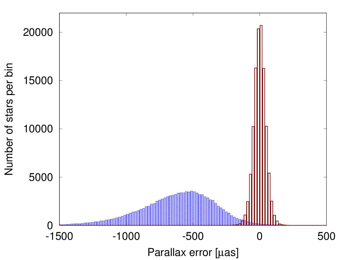
| 6–7 | 9 381 | 367 | 10 892 | 41 | 3 388 footnotemark: | 36 | 312 | 501 | 82 | - | 43 | 250a𝑎aa𝑎aCase B parallaxes are biased as shown in Fig. 2. This bias is not included in the RSE values given here. | 458 | 207 | - | 14 | 27 |
| 7–8 | 23 679 | 497 | 14 434 | 41 | 2 692 footnotemark: | 35 | 318 | 684 | 81 | - | 43 | 261a𝑎aa𝑎aCase B parallaxes are biased as shown in Fig. 2. This bias is not included in the RSE values given here. | 608 | 204 | - | 19 | 30 |
| 8–9 | 40 729 | 682 | 19 947 | 41 | 2 369 footnotemark: | 35 | 330 | 939 | 77 | - | 43 | 271a𝑎aa𝑎aCase B parallaxes are biased as shown in Fig. 2. This bias is not included in the RSE values given here. | 840 | 197 | - | 26 | 35 |
| 9–10 | 27 913 | 936 | 27 629 | 40 | 2 663 footnotemark: | 35 | 333 | 1 284 | 77 | - | 43 | 274a𝑎aa𝑎aCase B parallaxes are biased as shown in Fig. 2. This bias is not included in the RSE values given here. | 1 165 | 194 | - | 35 | 43 |
| 10–11 | 8 563 | 1 403 | 41 352 | 42 | 5 240 footnotemark: | 36 | 343 | 1 921 | 83 | - | 46 | 283a𝑎aa𝑎aCase B parallaxes are biased as shown in Fig. 2. This bias is not included in the RSE values given here. | 1 744 | 205 | - | 50 | 60 |
| 11–12 | 2 501 | 2 125 | 61 896 | 41 | 13 687 footnotemark: | 35 | 357 | 2 882 | 78 | - | 47 | 291a𝑎aa𝑎aCase B parallaxes are biased as shown in Fig. 2. This bias is not included in the RSE values given here. | 2 607 | 195 | - | 70 | 85 |
| 12 | 630 | 3 248 | 109 030 | 42 | 13 926 footnotemark: | 38 | 378 | 4 291 | 80 | - | 51 | 295a𝑎aa𝑎aCase B parallaxes are biased as shown in Fig. 2. This bias is not included in the RSE values given here. | 4 578 | 209 | - | 94 | 134 |
| all | 113 396 | 753 | 22 148 | 41 | 2 856 footnotemark: | 35 | 328 | 1 033 | 79 | - | 44 | 271a𝑎aa𝑎aCase B parallaxes are biased as shown in Fig. 2. This bias is not included in the RSE values given here. | 932 | 199 | - | 29 | 38 |
4.2 Predicted astrometric accuracies of htpm
Table 2 summarizes the results for the entire set of Hipparcos stars, and subdivided by magnitude. No results are given for the auxiliary stars, but they are similar to the results for the Hipparcos stars in the Gaia 12 scenarios. For comparison we also give the formal uncertainties from the Hipparcos Catalogue. For the positions they are given both at the original epoch J1991.25 and at the epoch J2015 of the Gaia data. It should be noted that the simulations include stars which in the Hipparcos Catalogue are described with more than five parameters, but are here treated as single stars. Excluding them from the statistics would systematically reduce the Hipparcos uncertainties in Table 2. The real htpm solution will also include all Hipparcos stars independent of the type of solution in the Hipparcos Catalogue. A poor fit between the Gaia and Hipparcos data will then be used to filter out binary candidates for further treatment.
All Gaia 12 and htpm uncertainties in Table 2 are derived from the distribution of the actual errors (calculated values minus true values) obtained in the solutions, using the “Robust Scatter Estimate” (RSE).888The RSE is defined as 0.390152 times the difference between the 90th and 10th percentiles of the distribution of the variable. For a Gaussian distribution it equals the standard deviation. Within the Gaia core processing community the RSE is used as a standardized, robust measure of dispersion (Lindegren et al. 2012). Rather than stating the uncertainty of and separately we give the mean of the RSE in the two coordinates as the position uncertainty. Similarly the proper motion uncertainty is the mean RSE of the errors in and .
Proper motion
The joint solution shows a big improvement in the proper motion uncertainties compared with the Hipparcos data. The improvement factor of htpm compared with Hipparcos alone is 32 in case A and 25 in case B. The factors are similar because the Hipparcos position uncertainty dominates over the Gaia uncertainty in both cases. In the optimistic case A, the proper motions from the Gaia-only data are already better than Hipparcos alone, but not as good as the joint htpm solution.
Using Eq. (3) to estimate the expected precision of the conventional combination we find in case A proper motions of 16 and 137 as yr-1 for the brightest and faintest magnitude bins, compared with 14 and 94 as yr-1 in the htpm-A results. In case B we find 143 and 602 as yr-1, respectively, compared with 27 and 134 as yr-1 in htpm-B. The joint solution thus gives consistently better results as discussed in Sect. 2.4.
Parallax
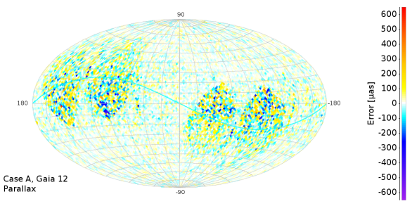
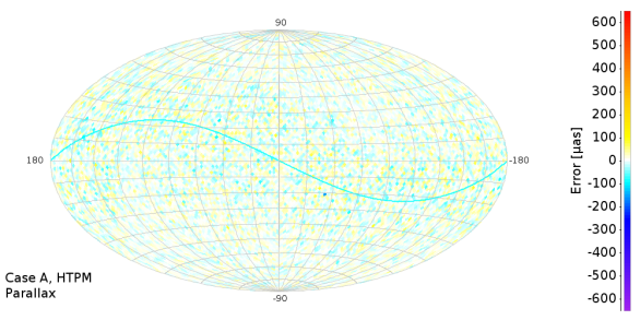
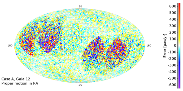
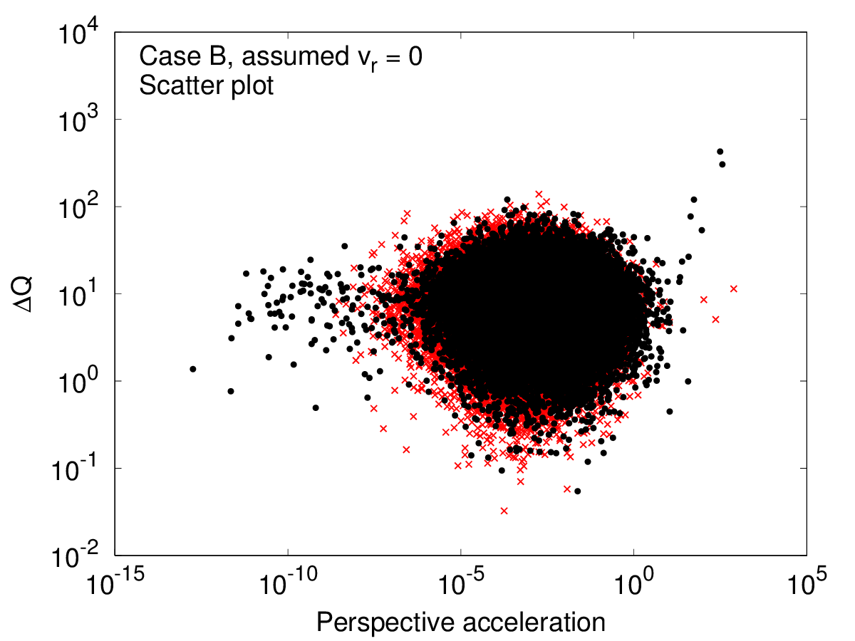
The improved proper motions allows better to disentangle the five parameters in the joint astrometric solution (cf. Fig. 3), resulting in improved parallax uncertainties. In case A we find that the parallax uncertainties in the joint solution improve by a factor 23 compared with Hipparcos, and a factor 2 compared with Gaia 12. However in the more realistic case B the improvement is much smaller (a factor 3 compared with Hipparcos) and the parallaxes are strongly biased as shown in Fig. 2. This bias originates from the assumption of zero parallax and proper motion in the two-parameter solution of the auxiliary stars. The true positive parallaxes result in a biased attitude, which propagates into the five-parameter solution of the Hipparcos stars making their parallaxes systematically too small. (As discussed in Sect. 5.2, this bias can be entirely avoided in later releases of Gaia data through a proper selection of primary sources.)
Position
The extremely good Gaia observations lead to an improvement by up to a factor 600 compared with Hipparcos positions propagated to J2015. In case A the slight improvement in the htpm positions compared with Gaia 12 comes from the better determination of proper motion and parallax. In case B the Gaia-only positions show a large uncertainty due to the two-parameter solution which neglects the true parallaxes and proper motions of the stars. The increase in position uncertainties is especially pronounced for the fainter stars due to preferential selection of nearby high-proper motion stars in the non-survey part of the Hipparcos Catalogue, which means that their (neglected) parallaxes and proper motions are statistically much larger than for the brighter (survey) stars. In the htpm solution for case B all five parameters are solved for the Hipparcos stars, so the sizes of their parallaxes and proper motions have no direct impact on the accuracy of the solution. However, the positional uncertainties are still much increased compared with case A, because the two-parameter solutions for the auxiliary stars degrade the attitude estimate.
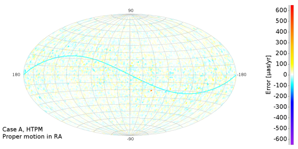
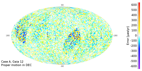
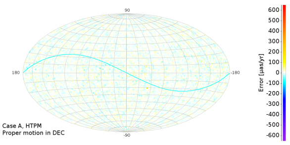
4.3 Goodness of fit statistics
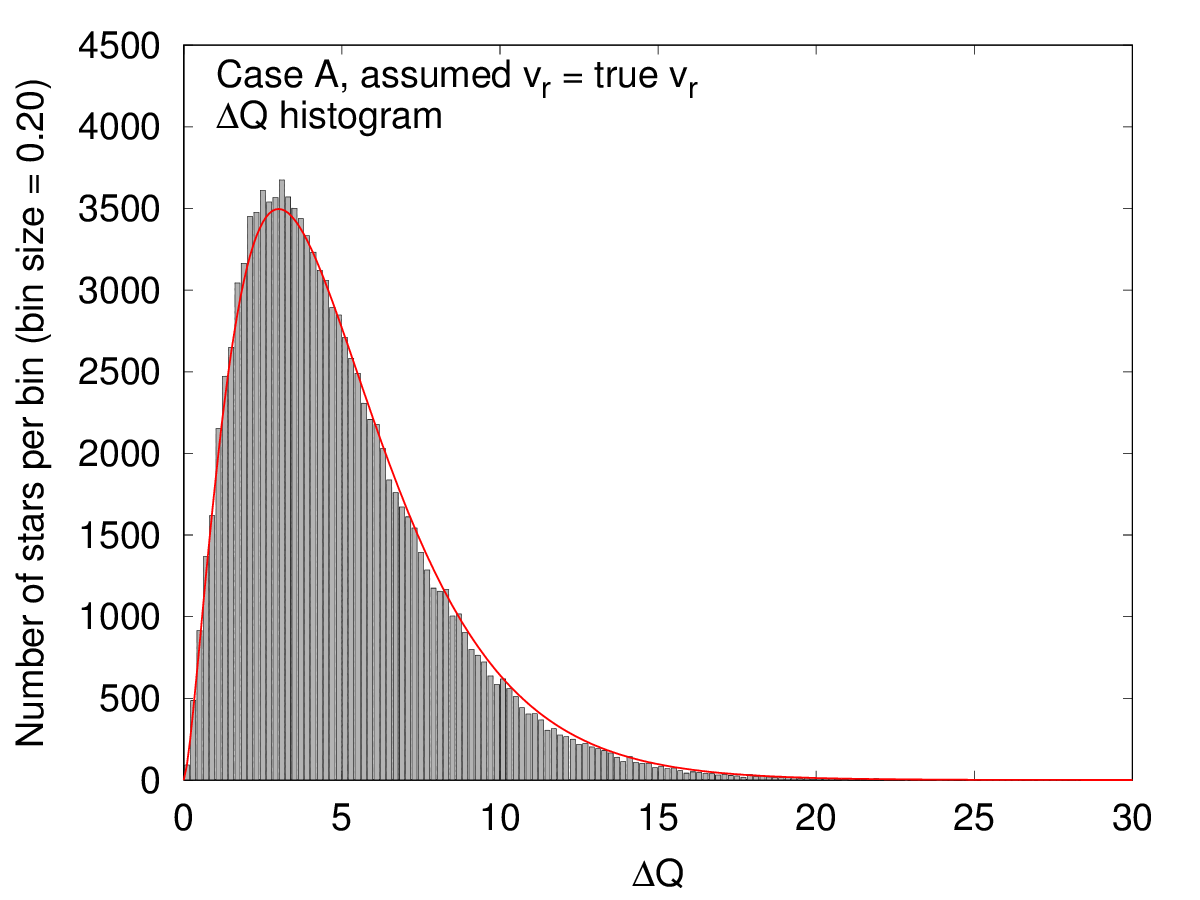
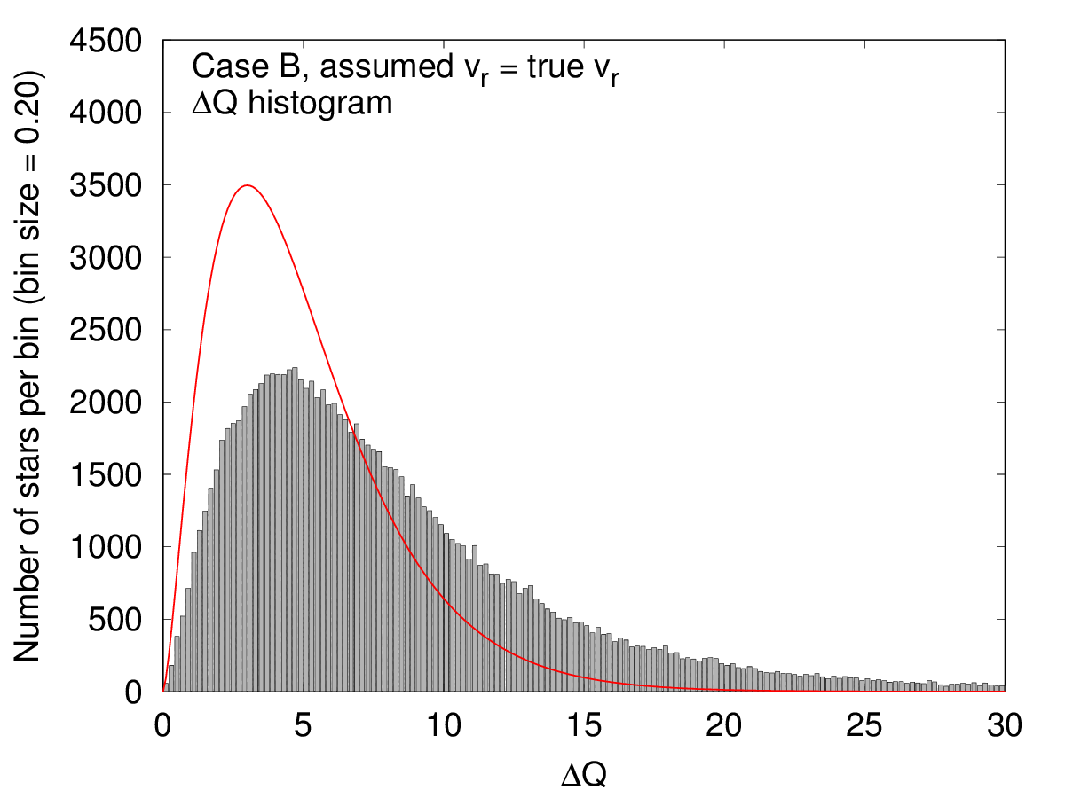
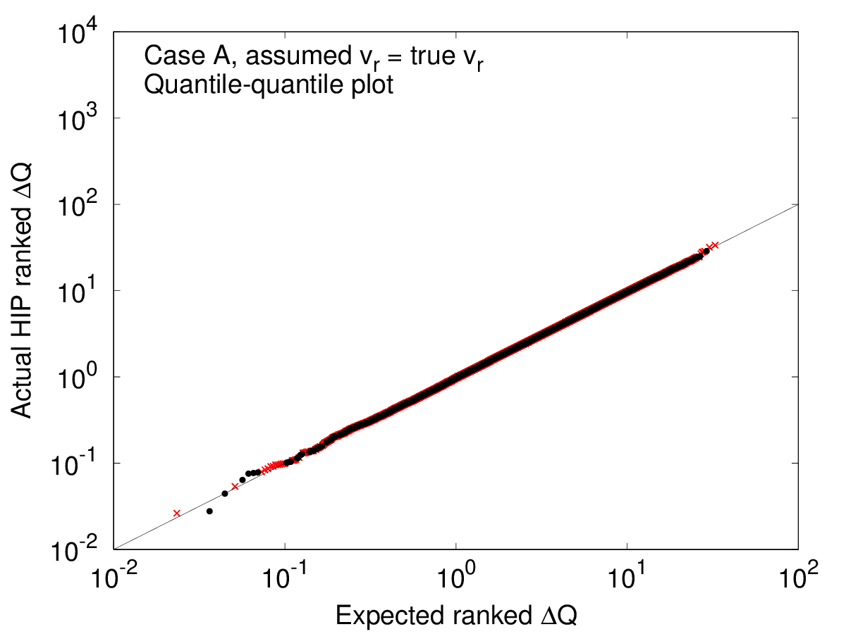
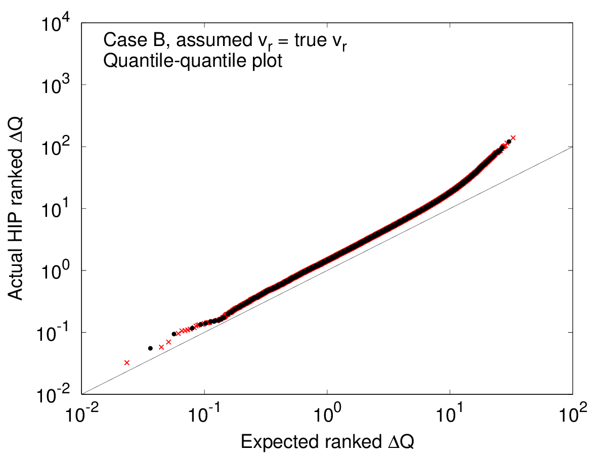


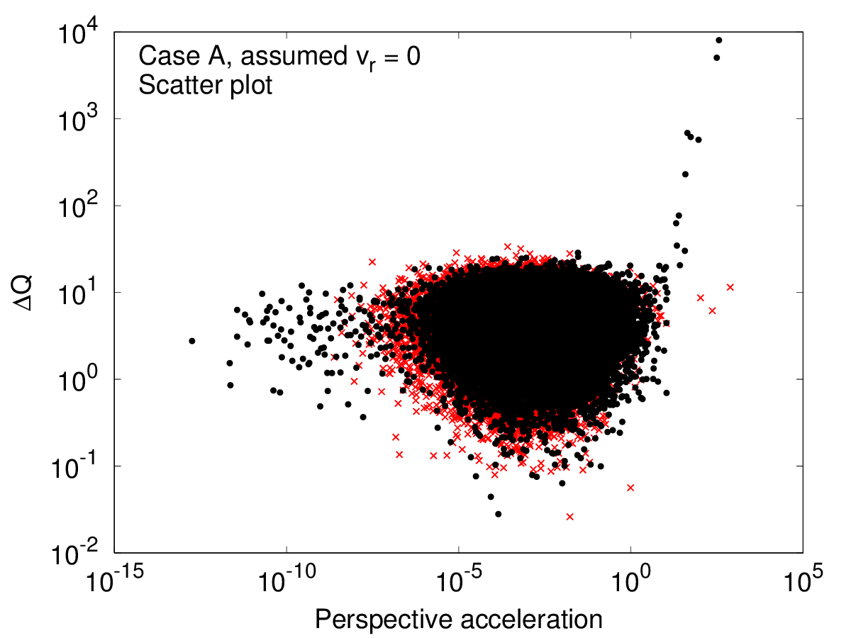
As discussed in Sect. 2.5 the goodness of fit value from Eq. (10) describes how well the joint astrometric solution fits the individual observations of both missions together. If all the observations are consistent with the kinematic model, then is expected to follow a distribution with five degrees of freedom. Larger values indicate deviations from the model, for example non-uniform motion caused by invisible companions or astrometric binaries. In the present simulations we do not include any such objects, so we expect to follow the theoretical distribution.
The top two diagrams in the left column in Fig. 4 shows that this is indeed true in case A, if the radial velocities assumed in the solution are the true ones. The result would have been the same if the assumed radial velocities had only been wrong by a few km s-1. If instead we assume zero radial velocities for all stars, as was done in the bottom two diagrams (while the observations were still generated with non-zero radial velocities), we find a small number of outliers. It turns out that all of them are nearby, high-velocity stars (Table 3) expected to show significant perspective acceleration, that is the change in proper motion due to the changing stellar distance and the changing angle between the line of sight and motion of the star (Schlesinger 1917; van de Kamp 1977; Murray 1983). This perspective acceleration is not taken into account in the solution when the radial velocities are assumed to be zero, giving a mismatch between the Hipparcos data and the observed Gaia position. The positional offset due to the perspective acceleration after years amounts to
| (20) |
where is the total proper motion. As shown in Table 3, the stars with a large also have a large offset at the Gaia epoch, compared with the positional uncertainty of the solution at that epoch.
This demonstrates that knowledge of radial velocities is required for a number of stars to avoid false positives in the detection of non-uniform space motion (de Bruijne & Eilers 2012). It also shows that is a useful statistic for detecting non-uniform space motion in general.
The right column in Fig. 4 shows the corresponding results in case B. Here follows a scaled version of the expected distribution with a somewhat extended tail. The two bottom panels show that is still a useful measure of deviations from the adopted kinematic model although it is much less sensitive than in case A. As a result only two outliers due to the perspective acceleration are found if the assumed radial velocities are set to zero. This demonstrates the strong dependency of on the quality of the Gaia solution.
| HIP | Remark | |||||||
|---|---|---|---|---|---|---|---|---|
| [mas ] | [mas yr-1] | [km s-1] | [mas yr-1] | [mas] | ||||
| 87937 | 8 044.46 | 9.490 | 548.31 | 10 358.94 | 361.87 | Barnard’s star | ||
| 24186 | 5 053.12 | 8.932 | 255.66 | 8 669.40 | 245.19 | 13 223.43 | 312.01 | Kapteyn’s star |
| 57939 | 686.11 | 6.564 | 109.99 | 7 059.03 | 43.72 | Groombridge 1830 | ||
| 104217 | 618.09 | 6.147 | 285.88 | 5 172.58 | 54.70 | 61 Cyg Ba𝑎aa𝑎a61 Cyg A (HIP104214) was not included in the simulations since it is brighter than the nominal Gaia bright star limit. | ||
| 54035 | 572.73 | 7.506 | 392.64 | 4 801.04 | 92.31 | |||
| 70890 | 229.59 | 10.761 | 771.64 | 3 852.57 | 38.32 | Proxima Centauri | ||
| 74235 | 76.86 | 9.200 | 34.65 | 3 681.26 | 310.12 | 2 266.79 | 24.80 | |
| 439 | 62.69 | 8.618 | 230.42 | 6 100.36 | 25.38 | 1 233.65 | 20.64 | |
| 74234 | 34.62 | 9.568 | 35.14 | 3 680.96 | 310.77 | 2 303.67 | 21.63 | |
| 54211 | 30.13 | 8.803 | 206.27 | 4 510.10 | 68.89 | 2 997.58 | 36.97 |
5 Discussion
5.1 Longevity of the htpm solution: detection of binary and exoplanetary candidates
As Gaia collects further data the accuracy of the proper motions determined from Gaia data alone will eventually supersede that of htpm. Assuming nominal mission performance and that the proper motion uncertainty scales with mission length as , this will happen already after 2–3 years of Gaia data have been accumulated. Still, htpm will remain a valuable source of information as it is based on a much longer time baseline. This is relevant for long period companions which create astrometric signatures that cannot be seen in Gaia data alone. We therefore suggest that htpm should be repeated with future Gaia releases. The goodness-of-fit of the combined solution is sensitive to small deviations of the stellar motions from the assumed (rectilinear) model. This sensitivity will dramatically increase with more Gaia data, namely when the Gaia-only proper motions become as good as the combined htpm proper motions.
The potential for detecting faint (stellar or planetary) companions to nearby stars can be illustrated by a numerical example. Consider a star at 10 pc distance ( mas) from the Sun, with an invisible companion of mass orbiting at a period of years (semi-major axis au). The astrometric signature of the companion (i.e., the angular size of the star’s orbit around their common centre of mass; Perryman 2014) is mas if the orbit is seen face-on, and the instantaneous proper motion of the star relative to the centre of mass is mas yr-1. If Hipparcos effectively measures this instantaneous proper motion which is extrapolated over years, the extrapolated position from Hipparcos (with its uncertainty of about 22 mas, see Table 2) and the position observed by Gaia (with an uncertainty much smaller than from Hipparcos) could differ by up to mas. Assuming that detection is possible if the position difference is at least twice as large as the positional uncertainty,101010Table 3 shows that in case A may be sensitive to positional deviations at the Gaia epoch as small as 21 mas. we find that the initial htpm results could be sensitive to companion masses down to , that is brown dwarf or super-Jupiter companions.
If we instead let Gaia measure the instantaneous proper motion of the system and propagate backwards to the Hipparcos epoch, we can take advantage of the much better uncertainties of the Gaia astrometry. Two to three years of Gaia data already give proper motion uncertainties better than as yr-1 for the bright stars, and hence extrapolated position uncertainties better than Hipparcos at its own epoch, or mas (Table 2). Therefore the htpm sensitivity increases roughly by a factor 30, allowing the detection of companion masses down to about , or Saturn-type objects at a Saturn-like distance to the host star.
This demonstrates that the results of htpm can be used to find candidates for long period exoplanets around nearby stars, with a highly interesting companion mass range opening up with subsequent releases of Gaia data when combined with Hipparcos. These companions cannot be detected from Gaia data alone even at the full mission length, and are hard to detect through classical methods due to their long periods, low transit probability and small radial velocity signatures. Since is sensitive to deviations from uniform space motion, whether they are seen in the Hipparcos or in the Gaia data, or both, this statistic can be used to find candidate systems in all these cases. The further exploration of the candidate systems will however require specialised analysis tools.
In a future publication we will explore in more detail how can be used to identify binary and exoplanetary candidates with orbital periods of decades to centuries. Apart from the possibility to detect sub-stellar companions for the nearest stars, this will contribute to the census of the binary population within a few hundred parsecs from the sun by filling a difficult-to-observe gap between the shorter period spectroscopic and astrometric binaries and the visually resolved long-period systems.
5.2 Two versus five parameters
When evaluating the results of our simulations, case B deserves additional attention since it is the more realistic case for the first Gaia data release, and the first simulation of this case published so far. The two-parameter solution (Gaia 12 B in Table 2) leads to a large position error of several mas. This is caused by assuming the parallax, proper and radial motion to be zero in the solution, whereas in reality they are not. The actual positional uncertainties in this case depend on the true distribution of parallaxes and proper motions for all the stars, including the auxiliary stars, which are not very well known. The numerical values given here are based on the very schematic distribution model for the auxiliary stars described in Sect. 3.2.1, and should therefore be interpreted with caution.
This position error is also relevant for the case B htpm scenario, where the solution of the auxiliary stars is two parameters only, but where one solves all five parameters for the Hipparcos stars while incorporating prior information from the Hipparcos Catalogue. The position error of the auxiliary stars causes a poor attitude determination. This in turn leads to increased errors in the case B htpm results (compare htpm B and A in Table 2), with a bias in the parallax errors (see Sect. 4 and Fig. 2). For a parallax-unbiased solution it is necessary to estimate all five parameters for all stars included in the solution. Any mixture in the estimation of five and two parameters in the same solution will lead to a bias in the resulting parallaxes. This is not only true for the htpm scenario described in this paper but also in all Gaia-only data releases. Referring to the terminology used in Sect. 6.2 of Lindegren et al. (2012), any star for which not all five astrometric parameters can be solved must be treated as a “secondary source”, meaning that it does not contribute to the attitude determination and instrument calibration. This is necessary in order to avoid biases for the stars where all five parameters are estimated.
5.3 Frame rotation of the combined solution
For the final agis solution of Gaia the reference frame will be established by means of quasars, both by linking to the optical counterparts of radio (VLBI) sources defining the orientation of the International Celestial Reference Frame, and by using the zero proper motion of quasars to determine a non-rotating frame.111111 The apparent proper motion of quasars due to the Galactocentric acceleration is expected to have an amplitude of 4 as yr-1 and is taken into account when determining the spin of the reference frame. This can also be done for earlier Gaia data releases, at least for the orientation part, while the shorter time span will limit the determination of the spin. It is desirable to rotate the htpm results into the same reference frame as used for the first Gaia data release. This must be done in two steps. First, a provisional htpm must be computed in the Hipparcos frame (as it will be when the Hipparcos data are used as prior, see Sect. 2.7), without imposing any other constraints on the frame. This solution will contain (many) non-Hipparcos stars with only Gaia observations which include a multitude of quasars. Their positions and proper motions are used in a second step to correct the provisional htpm (and other data in the same solution) for the estimated orientation and spin. Since the htpm solution is integrated in agis, the estimation and correction of the frame can be accomplished using the procedures and tools developed for agis (Lindegren et al. 2012, Sect. 6.1).
5.4 Other applications of the joint solution method
The joint solution is applicable also to other combinations of astrometric data. Here we give two examples.
Nano-JASMINE (Hatsutori et al. 2009; Yamada et al. 2013) is an ultra-small Japanese satellite, a technology demonstrator for the JASMINE series of near-infrared astrometry missions, scheduled for launch in 2015. It targets bright stars between magnitude and , although the exact limits are not yet determined. Based on current performance estimates the uncertainties in stellar parameters will be similar to or slightly worse than the uncertainties of the Hipparcos data. However the data will still be very valuable since astrometric catalogues are best at their respective epochs and Nano-JASMINE may be the only astrometric mission at its epoch observing the brightest stars in the sky. The Nano-JASMINE data can be analysed together with Hipparcos data analogously to the htpm project to improve the proper motions of bright stars that may not be observed by Gaia (Michalik et al. 2013).
The Tycho-2 Catalogue (Høg et al. 2000) gives positions for 2.5 million stars, derived from starmapper observations of Hipparcos. The positions at the reference epoch J1991.25 have a median internal standard error of 7 mas for stars brighter than mag and 60 mas for the whole catalogue. Combining the Tycho-2 positions with Gaia data using the joint solution scheme would allow us to derive proper motions for these stars with median uncertainties of 0.3 and 2.5 mas yr-1, respectively. This is true even in the conservative scenario (Gaia 12-B), since the major uncertainty comes from the Tycho-2 positions. In this combination the proper motions given in Tycho-2 should not be used, as they may contain systematic errors of a similar magnitude due to the incorporated old photographic material. The derived Tycho-Gaia Proper Motions (tgpm) catalogue however could be used to correct the photographic positions in order to take advantage of the much longer temporal baseline.
6 Conclusions
We have developed the joint solution method for incorporating priors in the core astrometric solution of Gaia. The method can be used in the processing of early Gaia data to improve the proper motions of the Hipparcos stars, the so-called Hundred Thousand Proper Motions project.
Combining astrometric data from very different epochs requires careful treatment of the non-linear effects of the mapping from spherical to rectilinear coordinates and for high velocity stars due to perspective acceleration. Therefore we have introduced a “scaled model of kinematics” (smok) which allows to handle these effects in a simple and rigorous manner.
Using simulations we have verified that htpm, using the joint solution method, gives the expected large improvements in proper motion uncertainties for over 100 000 stars in the Hipparcos Catalogue. The predicted proper motion uncertainties range from 14 to 134 as yr-1 depending on the amount of Gaia data used and the stellar magnitude, about a factor 30 improvement compared with the Hipparcos uncertainties.
We have shown that htpm also delivers improved parallaxes, which however may be strongly biased unless a full five-parameter solution can be obtained from Gaia-only data also for all non-Hipparcos stars. Whether these parallaxes should be published as part of an htpm release should be decided based on the amount and quality of Gaia data available at the time.
The joint solution is applicable also to a combination of Tycho-2 positions with early Gaia data to derive improved proper motions for the 2.5 million stars. We suggest that this possibility of a Tycho-Gaia Proper Motions (tgpm) catalogue should be considered in the Gaia data release plan.
The proposed method to calculate htpm provides a goodness-of-fit measurement which is sensitive to deviations from the uniform linear space motion. However, accurate radial velocities are required for nearby fast moving stars in order to avoid mistaking outliers in for companion signatures. We recommend to publish as well as the radial velocities used for the htpm data reduction. This will allow further investigations of outliers which might indicate binary or exoplanetary candidates, and will permit a correction of the htpm results if better radial velocities become available.
The full power of htpm will not be reached with the first Gaia data, but only in subsequent releases benefiting from the increased sensitivity of with improved Gaia results. Because of the long temporal baseline and the combination of current with historic astrometry, htpm will remain relevant throughout the final Gaia release for the detection and measurement of binary and exoplanetary candidates.
Acknowledgements.
We thank F. van Leeuwen for clarification on certain data items in the Hipparcos Catalogue and for providing valuable feedback as the referee. We also thank C. Fabricius for many useful comments. This work was partly carried out under ESA Contract No. 4000105564/12/NL/GE. Support from the Swedish National Space Board and the Royal Physiographic Society in Lund is gratefully acknowledged.References
- Abramowitz & Stegun (2012) Abramowitz, M. & Stegun, I. 2012, Handbook of Mathematical Functions (New York: Dover Publications)
- Anderson & Francis (2012) Anderson, E. & Francis, C. 2012, Astronomy Letters, 38, 331
- Bombrun et al. (2010) Bombrun, A., Lindegren, L., Holl, B., & Jordan, S. 2010, A&A, 516, A77
- Brinker & Minnick (1995) Brinker, R. C. & Minnick, R. 1995, The Surveying Handbook, 2nd ed. (Dordrecht: Kluwer)
- de Bruijne et al. (2010) de Bruijne, J., Siddiqui, H., Lammers, U., et al. 2010, in IAU Symposium, Vol. 261, Relativity in Fundamental Astronomy: Dynamics, Reference Frames, and Data Analysis, ed. S. A. Klioner, P. K. Seidelmann, & M. H. Soffel, 331
- de Bruijne & Eilers (2012) de Bruijne, J. H. J. & Eilers, A.-C. 2012, A&A, 546, A61
- Dehnen & Binney (1998) Dehnen, W. & Binney, J. J. 1998, MNRAS, 298, 387
- Dravins et al. (1999) Dravins, D., Lindegren, L., & Madsen, S. 1999, A&A, 348, 1040
- Eichhorn & Rust (1970) Eichhorn, H. & Rust, A. 1970, Astronomische Nachrichten, 292, 37
- ESA (1997) ESA. 1997, The Hipparcos and Tycho Catalogues (Noordwijk: ESA), ESA SP-1200
- Feissel & Mignard (1998) Feissel, M. & Mignard, F. 1998, A&A, 331, L33
- Hatsutori et al. (2009) Hatsutori, Y., Suganuma, M., Kobayashi, Y., et al. 2009, Transactions of Space Technology Japan, 7, 19
- Høg et al. (2000) Høg, E., Fabricius, C., Makarov, V. V., et al. 2000, A&A, 355, L27
- Holl et al. (2012) Holl, B., Lindegren, L., & Hobbs, D. 2012, A&A, 543, A15
- Lindegren et al. (2012) Lindegren, L., Lammers, U., Hobbs, D., et al. 2012, A&A, 538, A78
- Michalik et al. (2012) Michalik, D., Lindegren, L., Hobbs, D., Lammers, U., & Yamada, Y. 2012, in ASP Conference Series, Vol. 461, Astronomical Data Analysis Software and Systems XXI, ed. P. Ballester, D. Egret, & N. P. F. Lorente, 549
- Michalik et al. (2013) Michalik, D., Lindegren, L., Hobbs, D., Lammers, U., & Yamada, Y. 2013, in IAU Symposium, Vol. 289, Advancing the Physics of Cosmic Distances, ed. R. de Grijs, 414
- Mignard (2009) Mignard, F. 2009, The Hundred Thousand Proper Motions Project, Gaia Data Processing and Analysis Consortium (DPAC) technical note GAIA-C3-TN-OCA-FM-040
- Murray (1983) Murray, C. A. 1983, Vectorial astrometry (Bristol: Adam Hilger)
- Perryman (2014) Perryman, M. 2014, The Exoplanet Handbook (Cambridge, UK: Cambridge University Press)
- Risquez et al. (2013) Risquez, D., van Leeuwen, F., & Brown, A. G. A. 2013, A&A, 551, A19
- Schlesinger (1917) Schlesinger, F. 1917, AJ, 30, 137
- Taff (1981) Taff, L. G. 1981, Computational spherical astronomy (New York: Wiley-Interscience)
- van Altena (2013) van Altena, W. F. 2013, Astrometry for Astrophysics (Cambridge, UK: Cambridge University Press)
- van de Kamp (1977) van de Kamp, P. 1977, Vistas in Astronomy, 21, 289
- van Leeuwen (2007a) van Leeuwen, F. 2007a, Hipparcos, the New Reduction of the Raw Data, Astrophysics and Space Science Library, Vol. 350 (Springer)
- van Leeuwen (2007b) van Leeuwen, F. 2007b, A&A, 474, 653
- Wilson & Hilferty (1931) Wilson, E. B. & Hilferty, M. M. 1931, Proceedings of the National Academy of Science, 17, 684
- Yamada et al. (2013) Yamada, Y., Fujita, S., Gouda, N., et al. 2013, in IAU Symposium, Vol. 289, Advancing the Physics of Cosmic Distances, ed. R. de Grijs, 429
Appendix A Scaled Modelling of Kinematics (smok)
A formalism called Scaled Modelling of Kinematics (smok) is introduced in this paper to facilitate a rigorous manipulation of small (differential) quantities in the celestial coordinates. It is reminiscent of the “standard” or “tangential” coordinates in classical small-field astrometry (e.g., Murray 1983; van Altena 2013), using a gnomonic projection onto a tangent plane of the (unit) celestial sphere, but extends to three dimensions by adding the radial coordinate perpendicular to the tangent plane. This simplifies the modelling of perspective effects.
Figure 5 illustrates the concept. In the vicinity of the star let be a comparison point fixed with respect to the Solar System Barycentre (SSB). As shown in the diagrams:
-
1.
The barycentric motion of the star is scaled by the inverse distance to , effectively placing the star on or very close to the unit sphere.
-
2.
Rectangular coordinates are expressed in the barycentric system with pointing towards , and , in the directions of increasing right ascension and declination.
The first point eliminates the main uncertainty in the kinematic modelling of the star due to its poorly known distance. The second point allows us to express the scaled kinematic model in smok coordinates , , that are locally aligned with , , and the barycentric vector.
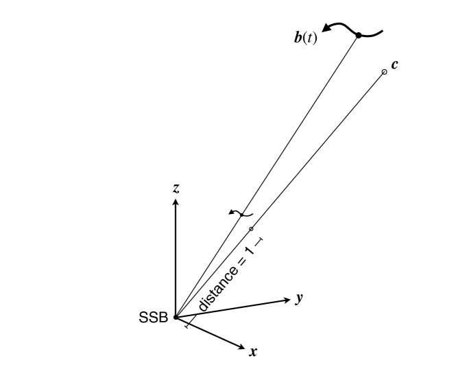
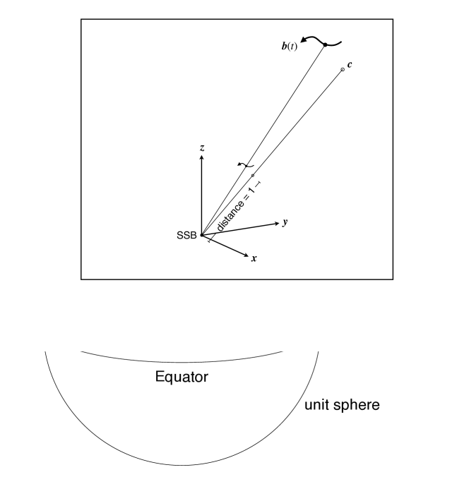
Up to the scale factor discussed below, the smok coordinate system is completely defined by the adopted comparison point using the orthogonal unit vectors
| (21) |
is the “normal triad” at the comparison point with respect to the celestial coordinate system (Murray 1983).121212 and point to the local “East” and “North”, respectively, provided that . However, the coordinate triad in Eq. (21) is well-defined even exactly at the poles, where remains significant for defining and . We are free to choose as it will best serve our purpose, but once chosen (for a particular application) it is fixed: it has no proper motion, no parallax, and no associated uncertainty. Typically is chosen very close to the mean position of the star.
The motion of the star in the Barycentric Celestial Reference System (BCRS) is represented by the function , where is the vector from SSB to the star as it would be observed from the SSB at time . The scaled kinematic model is given in smok coordinates as
| (22) |
and can in turn be reconstructed from the smok coordinates as
| (23) |
, , are dimensionless and the first two are typically small quantities (), while is very close to unity.
The whole point of the scaled kinematic modelling is that can be described very accurately by astrometric observations, even though may be poorly known due to a large uncertainty in distance. This is possible simply by choosing the scaling such that at some suitable time. This works even if the distance is completely unknown, or if it is effectively infinite (as for a quasar).
The scale factor is , where is the parallax of and the astronomical unit. The measured parallax can be regarded as an estimate of .
In the following we describe some typical applications of smok coordinates.
A.1 Uniform space motion
The simplest kinematic model is to assume that the star moves uniformly with respect to the SSB, that is
| (24) |
where is the barycentric position at the reference epoch , and is the (constant) space velocity. The scaled kinematic model expressed in the BCRS is
| (25) |
where
| (26) |
and
| (27) |
are constant vectors. The uniform motion can also be written in smok coordinates as
| (28) |
The six constants , , , , , are the kinematic parameters of the scaled model; however, to get the actual kinematics of the star we also need to know .
A.2 Relation to the usual astrometric parameters
Choosing to be the barycentric celestial coordinates of the star at , and equal to the parallax at the same epoch, we find
| (29) |
where , are the tangential components of the barycentric proper motion at the reference epoch , and is the “radial proper motion” allowing to take the perspective effects into account. is usually calculated from the measured radial velocity and parallax according to Eq. (1).
A.3 Differential operations
Uniform space motion does not map into barycentric coordinates , that are linear functions of time. The non-linearity derives both from the curvilinear nature of spherical coordinates and from perspective foreshortening depending on the changing distance to the object. Both effects are well known and have been dealt with rigorously by several authors (e.g., Eichhorn & Rust 1970; Taff 1981). The resulting expressions are non-trivial and complicate the comparison of astrometric catalogues of different epochs. For example, approximations such as
| (30) |
cannot be used when the highest accuracy is required. By contrast, the linearity of Eq. (28) makes it possible to write
| (31) |
to full accuracy, provided that the same comparison point is used for both epochs. (Strictly speaking, the same scale factor must also be used, so that in general .) If the position at the reference epoch coincides with the comparison point used, the resulting , are the looked-for proper motion components according to Eq. (29); otherwise a change of comparison point is needed (see below).
A.4 Changing the comparison point
Let and be different comparison points with associated triads and . If , , and , , describe the same scaled kinematics we have by Eq. (23)
| (32) |
Thus, given , , one can compute from the first equality in Eq. (32), whereupon the modified functions are recovered as
| (33) |
This procedure can be applied to for any particular as well as to linear operations on such as differences and time derivatives.
A.5 Epoch propagation
An important application of the above formulae is for propagating the six astrometric parameters , referring to epoch , to a different epoch . This can be done in the following steps:
-
1.
Use as the comparison point and compute by Eq. (21). At time the smok parameters relative to the first comparison point are , , , , .
- 2.
-
3.
Calculate by means of Eq. (25). Let be its length (close to unity).
-
4.
Calculate and hence the second comparison point and triad .
-
5.
Use Eq. (33) to calculate the smok parameters at referring to the second comparison point. For the position one trivially gets and . For the proper motion parameters one finds , , and .
-
6.
The astrometric parameters at epoch are , , , , , .
This procedure is equivalent to the one described in Sect. 1.5.5, Vol. 1 of The Hipparcos and Tycho Catalogues (ESA 1997).
Appendix B The Hipparcos Catalogue
This Appendix describes the calculation of relevant quantities from the new reduction of the Hipparcos Catalogue by van Leeuwen (2007b). Data files were retrieved from the Strasbourg astronomical Data Center (CDS) in November 2013 (catalogue I/311). These files differ slightly from the ones given on the DVD published along with the book (van Leeuwen 2007a), both in content and format, as some errors have been corrected. The data needed for every accepted catalogue entry are:
-
•
the five astrometric parameters ;
-
•
the normal matrix from the least-squares solution of the astrometric parameters (for a 5-parameter solution this equals the inverse of the covariance matrix );
-
•
the chi-square goodness-of-fit quantity for the 5-parameter solution of the Hipparcos data;
-
•
the degrees of freedom associated with .
The astrometric parameters at the Hipparcos reference epoch J1991.25 are directly taken from the fields labelled RArad, DErad, Plx, pmRA, and pmDE in the main catalogue file hip2.dat. Units are [rad] for and , [mas] for , and [mas yr-1] for and . It is convenient to express also positional differences (such as smok coordinates and ) and positional uncertainties in [mas]. The elements of thus have units [mas-2 yr], where , 1, or 2, depending on the position of the element in the matrix.
The calculation of , , and is described hereafter in some detail as the specification of deviates in some details from the published documentation. Clarification on certain issues was kindly provided by F. van Leeuwen (private comm.).
The number of degrees of freedom is
| (34) |
where is the number of field transits used (label Ntr in hip2.dat) and is the number of parameters in the solution (see below; most stars have ). The goodness-of-fit given in field F2 is the “gaussianized” chi-square (Wilson & Hilferty 1931)
| (35) |
computed from , the sum of the squared normalized residuals, and . For “good” solutions is expected to follow the chi-square distribution with degrees of freedom (), in which case approximately follows the standard normal distribution, . Thus, means that is “too large” for the given at the same level of significance as the criterion for a Gaussian variable (probability ).131313This transformation was also used to generate the F2 statistic given in field H30 of the Hipparcos and Tycho Catalogues (ESA 1997). Given from field F2, and from Eq. (34), it is therefore possible to reconstruct the chi-square statistic of the -parameter solution as
| (36) |
We also introduce the square-root of the reduced chi-square,
| (37) |
which is expected to be around 1.0 for a “good” solution (see further discussion below). is sometimes referred to as the standard error of unit weight (Brinker & Minnick 1995).
The catalogue gives the covariance matrix in the form of an upper-diagonal “weight matrix” such that, formally, . This inverse exists for all stars where a solution is given. (For the joint solution we actually need the normal matrix , see below.) For solutions with astrometric parameters there are non-zero elements in . For some stars the solution has more than five parameters, and the main catalogue then only gives the first 15 non-zero elements, while remaining elements are given in separate tables. Let , , , be the 15 values taken from the fields labelled UW in hip2.dat. The matrix is computed as
| (38) |
Here , , are scaling factors which for the CDS data must be calculated as
| (39) | ||||||||
where is given by Eq. (37) and are the standard errors given in fields e_RArad through e_pmDE of hip2.dat. Equation (B) applies to data taken from the CDS version of the catalogue (I/311). For catalogue data on the DVD accompanying the book (van Leeuwen 2007a), scaling factors apply, although those data are superseded by the CDS version.
The matrix computed using the first five rows and columns in , as given in Eq. (38), contains the relevant elements of the normal matrix for any solution with . Thus, for solutions with there is no need, for the catalogue combination, to retrieve the additional elements of from hip7p.dat, etc. The situation is different when the covariance matrix is needed: it is then necessary to compute the full normal matrix before can be computed.
The normal matrix computed as described above incorporates the formal uncertainties of the observations; as described in van Leeuwen (2007a) these are ultimately derived from the photon statistics of the raw data after careful analysis of the residuals as function of magnitude, etc. If the adopted models are correct we expect the statistic to be normally distributed with zero mean and unit standard deviation, and the standard error of unit weight, , to be on the average equal to 1. In reality we find (for solutions with ) that their distributions are skewed towards larger values, especially for the bright stars where photon noise is small and remaining calibration errors are therefore relatively more important. To account for such additional errors the published standard errors , etc., in hip2.dat include, on a star-by-star basis, a correction factor equal to the unit weight error obtained in its solution. This is equivalent to scaling the formal standard errors of the data used in the solution by the same factor. In order to make the computed normal matrix, covariance matrix, and goodness-of-fit statistics consistent with the published standard errors it is then necessary to apply the corresponding corrections, viz.:
| (40) |
For the catalogue combination we use and whenever , but and if .