A Mathematical Model of Flavescence Dorée Epidemiology

Abstract

Flavescence dorée (FD) is a disease of grapevine transmitted by an insect vector, Scaphoideus titanus Ball. At present, no prophylaxis exists, so mandatory control procedures (e.g. removal of infected plants, and insecticidal sprays to avoid transmission) are in place in Italy and other European countries. We propose a model of the epidemiology of FD by taking into account the different aspects involved into the transmission process (acquisition of the disease, latency and expression of symptoms, recovery rate, removal and replacement of infected plants, insecticidal treatments, and the effect of hotbeds). The model was constructed as a system of first order nonlinear ODEs in four compartment variables. We perform a bifurcation analysis of the equilibria of the model using the severity of the hotbeds as the control parameter. Depending on the non-dimensional grapevine density of the vineyard we find either a single family of equilibria in which the health of the vineyard gradually deteriorates for progressively more severe hotbeds, or multiple equilibria that give rise to sudden transitions from a nearly healthy vineyard to a severely deteriorated one when the severity of the hotbeds crosses a critical value. These results suggest some lines of intervention for limiting the spread of the disease.
keywordsFlavescence dorée Grapevine epidemiology Critical transition Fold bifurcation Scaphoideus titanus Ball

1 Introduction

Flavescence dorée (hereafter FD) is a serious disease of grapevine, widespread in many European countries, caused by phytoplasmas belonging to 16SrV-C and 16SrV-D ribosomal groups [1]. Symptoms of FD include leaf yellowing or redness, lack of lignification of canes, lack of blossom, and so on. The infected plants stop to produce grapes, and die after a few years. Symptoms of FD are usually shown after a latency period of 1-3 years from infection; young plants are more likely to show symptoms just one year after infection [3, 2].

FD is transmitted vine-to-vine by an insect vector, Scaphoideus titanus Ball (Hemiptera: Cicadellidae), native to North America and introduced into Europe in the late 1950s [4, 17]. S. titanus feeds and reproduces only on grapevine (Vitis spp.), has a single generation per year, and overwinters in the egg stage, laid under the bark of grapes [5, 17]. Eggs start to hatch during spring, and the insect over-goes through five nymphal instars before becoming adult during summer [5, 6]. Nymphs from the 3rd and later instars acquire phytoplasmas when feeding on infected plants, and after a latency period lasting 4-5 weeks (meanwhile becoming adults) they are able to inoculate phytoplasmas to healthy plants [7]. Once infective, insects retain vector capability through their lifetime; on the other hand, no transovarial transmission has been proved for S. titanus at present, therefore newly born insects have to feed on infected plants in order to acquire phytoplasmas [8]. Other insects are acknowledged to be occasional vectors [9], however their role in the spread of Flavescence dorée to date is not considered to be important.

Infected plants may be subject to recovery, with symptoms disappearing within a few years after the infection with recovery rates that depend on cultivar and age of plants, the youngest being the less able to recover [3]. Observed recovery rates are highly variable and range from 1% to 70% of the infected plants, but show a strong inverse dependence on the abundance of the vector insect, with the highest recovery rates observed in vineyards subject to aggressive insecticide treatments, and the lowest in vineyards subject to no treatments [3, 10]. This supports the notion that recovered plants are not immune from reinfection. However, recovered plants are not a source of phytoplasmas for insects [11].

In Italy FD is subject to mandatory control procedures, including sprays of insecticide against the vector and removal of the infected plants, which, however, may have higher cost than insecticide treatment. In many vine-growing areas abandoned vineyards and woods containing wild grapevine act as hotbeds of both phytoplasmas and S. titanus [12, 13]. Adults of S. titanus are able to move from untreated to treated vineyards up to a distance of about 300 m [13].

In this paper we model the dynamics of the spread of FD over time, by considering the different aspects involved into (or influencing the) transmission process. The model could be used for forecasting the epidemiology of FD in a vineyard, given the knowledge of some parameters. More importantly, it highlights the key ecological factors involved in the infection process, and thus it offers guidance for planning an adequate response.

From a mathematical point of view, the model is a system of nonlinear, first-order, ordinary differential equations in the compartments $S$, $L$, $I$, $G$, modelling the dynamical behaviour of healthy full-grown, latent, infected and young (nursery) plants, respectively.

The rest of the paper is structured as follows. In Section 2 we formulate the model and present the main mathematical results. In Section 3 we discuss the ecological significance of those results. Conclusions are given in Section 4. The Appendix 5 contains proofs and other mathematical details that, for brevity and clarity, were omitted in the main text.

2 The model

2.1 Formulation

Previous modeling efforts have focused on the life-cycle of the S. titanus with the goal of optimizing the timing of pest management operations [14]. Models of this kind encompass a time frame of less than one year and are unable to describe the long-term evolution of an infested vineyard. In spite of the complicated life cycle, the year-to-year population levels of S. titanus in a vine growing area remains roughly constant, or at least of the same degree of magnitude, if all known relevant factors (e.g. timing, number and effectiveness of insecticidal sprays, the presence of nearby hotbeds of infestation) are kept constant. [15, 16, 14]. Therefore, for time scales longer than one year, it seems to be reasonable to formulate a continuous-time model whose variables are representative of plants densities in a vineyard, and where the insect vector does not appear explicitly, but is parameterized by a coupling term between the infected and the healthy plants.

Our model splits the grapevine population of a vineyard in four compartments (or stages), as shown in Figure

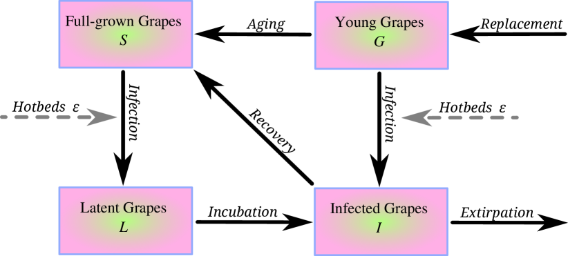
Figure 1: Graphical representation of the model. The grapevine population in a vineyard is split into four compartments, representing healthy, full-grown plants ($S$), healthy, young plants ($G$), latent plants ($L$) and infected plants ($I$). The solid black arrows represent the processes that increase (inward arrow) or decrease (outward arrow) the population of each compartment. The dashed gray arrows represent the effect of infection hotbeds close to the vineyard, triggering the infection fluxes in initially healthy vineyards.

1. The variable $S$ represents the density of healthy, full-grown plants (number of vines per unit area), and $I$ represents the density of infected plants. Because of the lack of transovarial transmission [8], individuals of S. titanus become vectors of the phytoplasma by feeding on infected plants. This occurs at the nymph stage, when the insect lacks the ability to move from plant to plant [17]. Therefore, after the eclosion, the abundance of mobile, phytoplasma-carrying adults will be proportional to the number of infected plants. Thus infection rate of the healthy plants should be modeled by a term of the form

$$\mathrm{Infection\,\,rate}=f(I)S$$ (1)

where $f$ is an unknown function that quantifies the efficiency of phytoplasma-carrying adults at infecting healthy plants. Obviously, $f$ must be a monotonically growing function of the density of infected plants, with $f(0)=0$. Laboratory experiments show that a small, but non-negligible fraction of plants remains healthy, after a relatively long exposure to a population fully composed by infected insects [18]. This suggests that many probes from infected adults may be required for a plant to eventually contract FD. If this hypothesis is correct, then small numbers of infected plants in a vineyard should not be very effective at spreading the disease, because the small number of phytoplasma-carrying adults originating from those plants would feed on many different healthy plants during their lifespan, and only rarely return on the same plant enough times to infect it. Thus we argue that also the derivative of $f$ vanishes for $I\to 0$. Of course, if the density of infected plants is large, the probability of recurrent feeding on the same healthy plant of phytoplasma-carrying insects must be large as well. Thus we argue that $f$ should grow faster than linearly with $I$, at least at moderately low values of $I$. The simplest mathematical expression that captures these assumptions is

$$\mathrm{Infection\,\,rate}=qSI^{2}$$ (2)

where $q$ is a constant whose value depends on the susceptibility to the infection of the particular cultivar which is being considered, and on the local abundance of S. titanus. The value of this constant is subject to large uncertainties. We estimate $q\approx 10^{-6}$ $\mathrm{ha^{2}}$ $\mathrm{plants^{-2}}$ $\mathrm{Y^{-1}}$ , but reasonable values range from $10^{-7}$ to $10^{-5}$ $\mathrm{ha^{2}}$ $\mathrm{plants^{-2}}$ $\mathrm{Y^{-1}}$ (see Appendix 5.1 for details). The effect of insecticide treatments is that of lowering the value of $q$. This is discussed in Section 3.2.

Table 1: Value (or range of likely values) for the parameters appearing in the model (3).

Process	Parameter	Value	Reference
Farmer’s intervention time	$\tau$	$1\,\mathrm{Y}$	In Italy immediate eradication of infected plants is mandatory by law (DM 32442/2000). Similar measures are in place in France.
Vineyard’s design density	$D$	$2000\,\mathrm{to}\,11000\,\mathrm{plants/ha}$
Coupling infected-healthy	$q$	$10^{-6}\,(10^{-7}\,\mathrm{to}\,10^{-5})\,\mathrm{ha^{2}plants{}^{-2}\,Y^{-1}}$
Recovery from infection	$k_{1}$	${\displaystyle 0.4\,\mathrm{Y}^{-1}}$	[10]
Latency before symptoms	$k_{2}$	${\displaystyle\frac{1}{3}\,\mathrm{Y}^{-1}}$	[2, 3]
Mortality of infected plants	$k_{3}$	$\begin{cases}\tau^{-1}&\mathrm{(managed\;vineyards)}\\ 0.1\,\,\mathrm{Y}^{-1}&\mathrm{(unmanaged\;vin.)}\end{cases}$	By law (DM 32442/2000) Our estimate
Aging of new plants	$k_{4}$	${\displaystyle\frac{1}{5}\,\mathrm{Y}^{-1}}$	[3]

Because direct laboratory measurements of $f$ are presently lacking, we have resisted the temptation of using more complicated functional forms that, for example, let $f$ taper off (and maybe approach a horizontal asymptote) as $I$ increases. At the end of Section 3 we discuss the effect of choosing $f$ proportional to $I$.

In the presence of hotbeds of infection nearby the modeled vineyard (such as infected wild grapes or an abandoned infected vineyard), the density of infected plants that enters in the infection rate terms should not be $I$, but rather $(I+\varepsilon)$, where the parameter $\varepsilon$ quantifies the phytoplasma-carrying insects coming from the hotbeds, which appears to decay exponentially with the distance of the hotbed [13].

In time, some infected plants have a chance to recover from the disease, and to return symptom-free. Furthermore, they may be re-infected, thus recovered plants do not require a separate compartment. The process of recovery is modeled by a flux from the $I$ to the $S$ compartments quantified as $k_{1}I$. Experimental data, taken in vineyards where insecticide treatments had brought to a negligible amount the presence of S. titanus, show that the constant $k_{1}^{-1}$ ranges between $2$ and $3$ years for the popular Barbera and Sauvignon cultivars [10]. For other cultivars these figures should be taken as representative of the order of magnitude, and not as accurate estimates of the recovery rate.

In full-grown plants, the symptoms of FD do not usually appear immediately after the inoculation. Inoculated individuals may remain in a latent, symptomless state for up to a few years. In our model the density of latent plants is quantified by the compartment $L$. The amount of latent plants that develops symptoms is quantified by the flux $k_{2}L$ from the $L$ to the $I$ compartments. The time scale $k_{2}^{-1}$ of the process is estimated to be approximately $3$ years [2, 3].

We assume that the farmer extirpates actively the infected plants, on a time scale $k_{3}^{-1}=\tau$. This causes a mortality of the infected plants quantified as $-k_{3}I$. On the same time scale, the manager attempts to maintain a constant density $D$ of plants in the vineyard, by planting healthy, young plants, whose density is quantified by the variable $G$. This process continues as long as the actual density of the vineyard (which is $S+L+I+G$) doesn’t match the desired density $D$. The constant $\tau$ quantifies the reaction time of the farmer. While $\tau$ can’t be smaller than one year (infected grapes are roughed at the end of summer, and nursery grapes are usually planted in the next spring in order to be productive in autumn) it may occasionally be larger, when economic constraints force a delay of the extirpation and replacement procedures. Young plants are subject to infection just in the same way as full-grown ones, with the only difference that they do not have a phase of latency, but develop the symptoms rapidly after acquiring the phytoplasma [3]. Thus, the process of infection produces a flux from $G$ to $I$ (rather than to $L$). The infection rate of young plants is quantified as $qG(I+\varepsilon)^{2}$, analogously to (2). In principle we could model a different susceptibility to the infection for the young and the full-grown plants by using different values of the constant $q$ for the two compartments. However, lacking a direct empirical evidence of an evident disparity in susceptibility between young and full-grown plants, for simplicity, we prefer to use the same value of $q$ for both. Young plants that do not become infected eventually turn into full-grown plants by aging. This process is modeled as a flux from the $G$ to the $S$ compartment quantified as $k_{4}G$. For most cultivars the aging time is about $k_{4}^{-1}\approx 5$ years [3].

The model as described by the above considerations is embodied by the following system of first-order ordinary differential equations:

$$\begin{cases}S^{\prime}=&-qS\left(I+\varepsilon\right)^{2}+k_{1}I+k_{4}G\\ L^{\prime}=&\hphantom{-}qS\left(I+\varepsilon\right)^{2}-k_{2}L\\ I^{\prime}=&\hphantom{-}qG\left(I+\varepsilon\right)^{2}+k_{2}L-k_{1}I-k_{3}I\\ G^{\prime}=&-qG\left(I+\varepsilon\right)^{2}-k_{4}G+\\ &\hphantom{-}\tau^{-1}\left(D-S-L-I-G\right)\end{cases}$$ (3)

where the dot denotes differentiation with respect to time.

In Table 1 we summarize the above best-guesses of the values (or value range) of the constants, deduced from evidence given in the accompanying references.

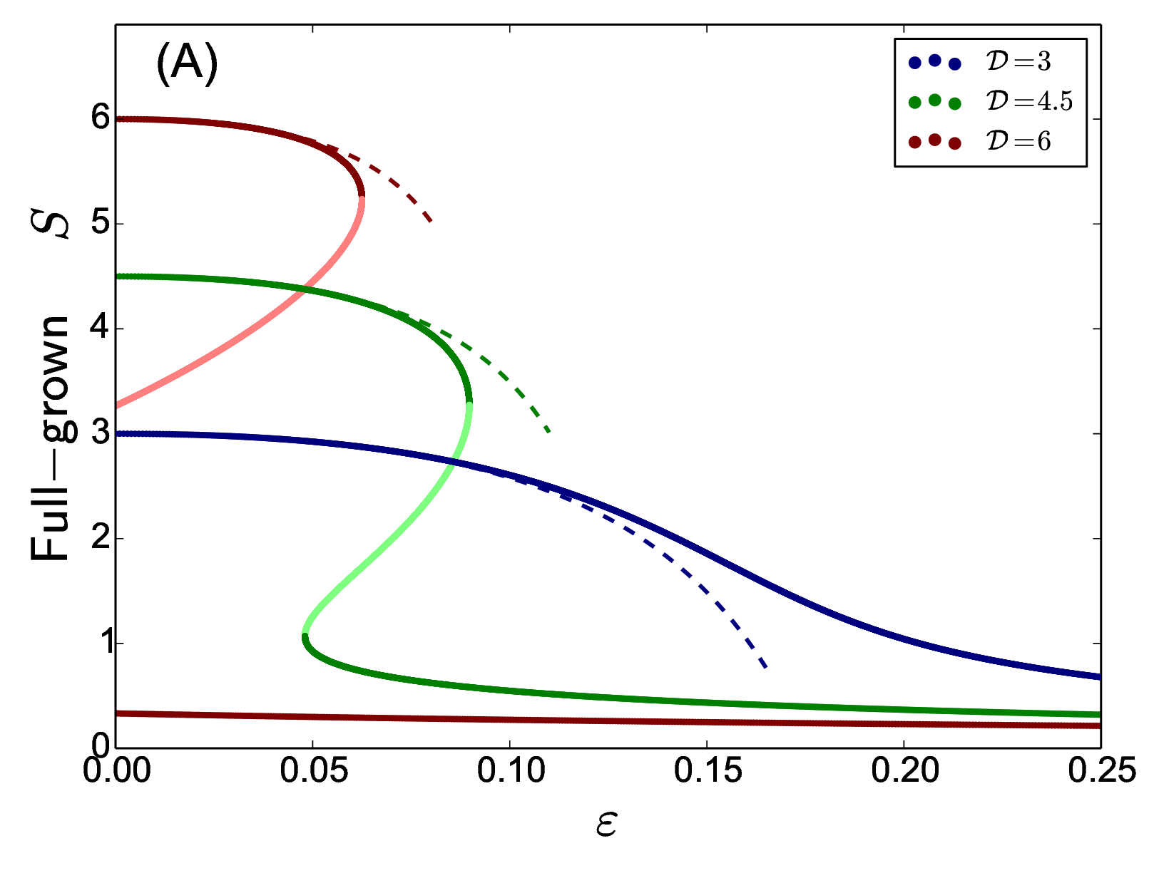
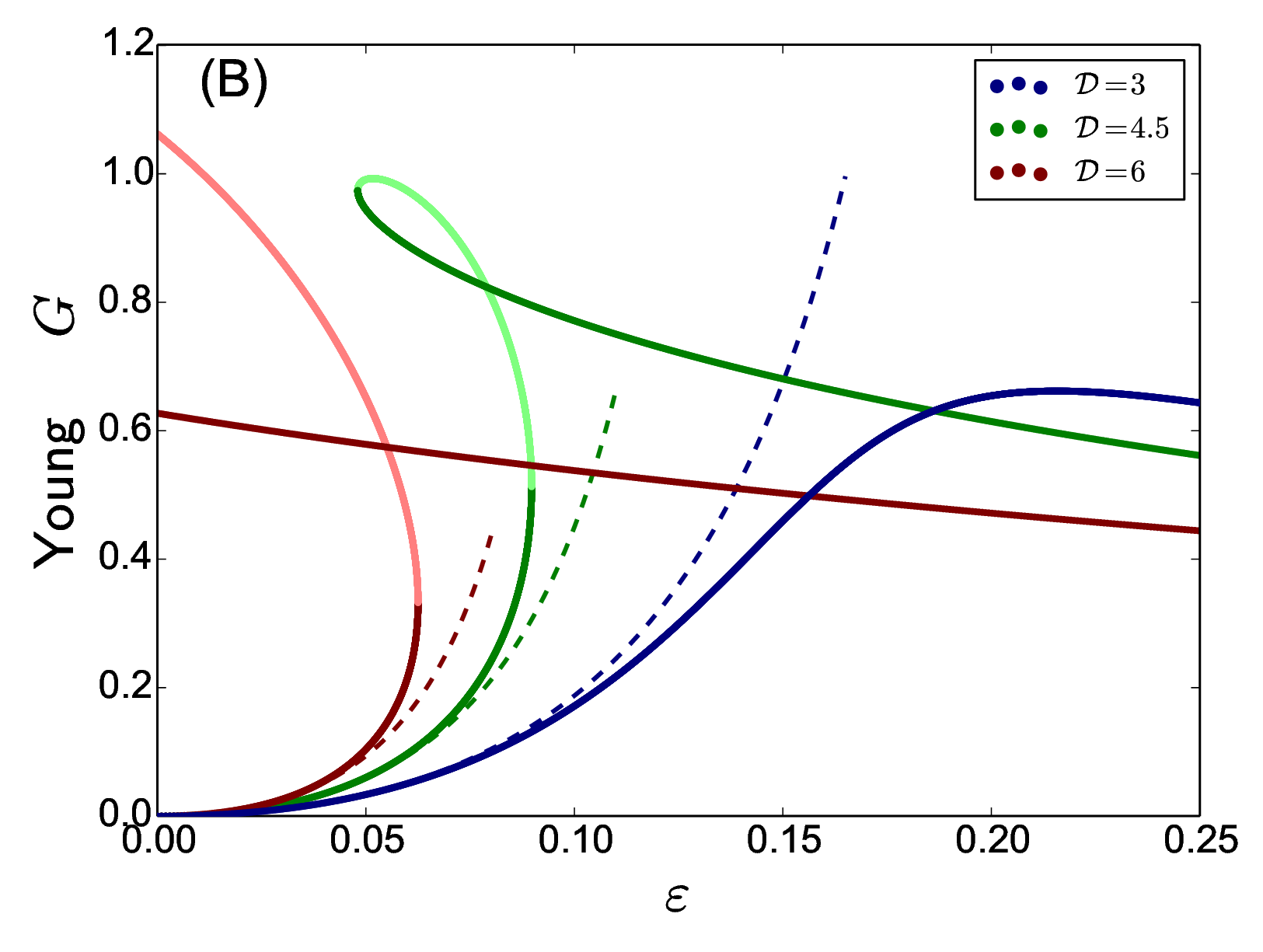
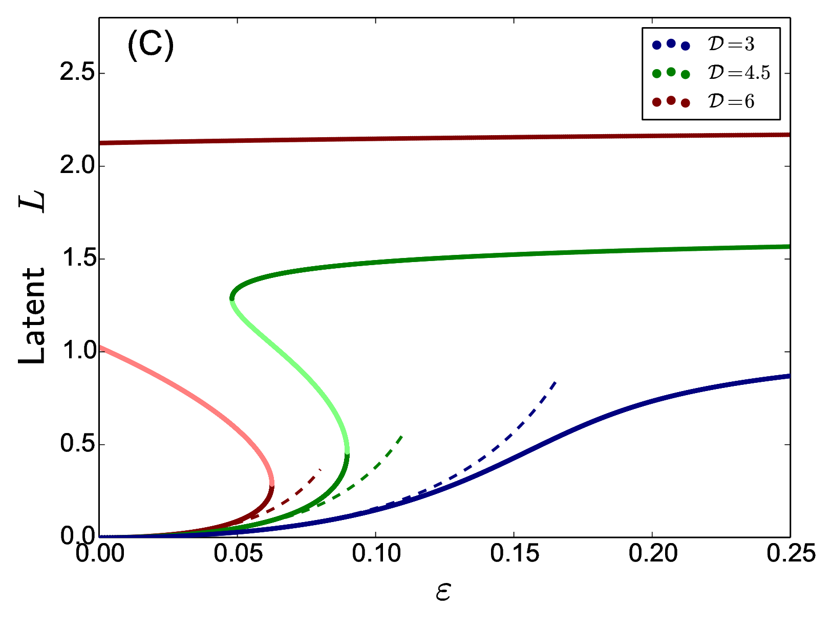
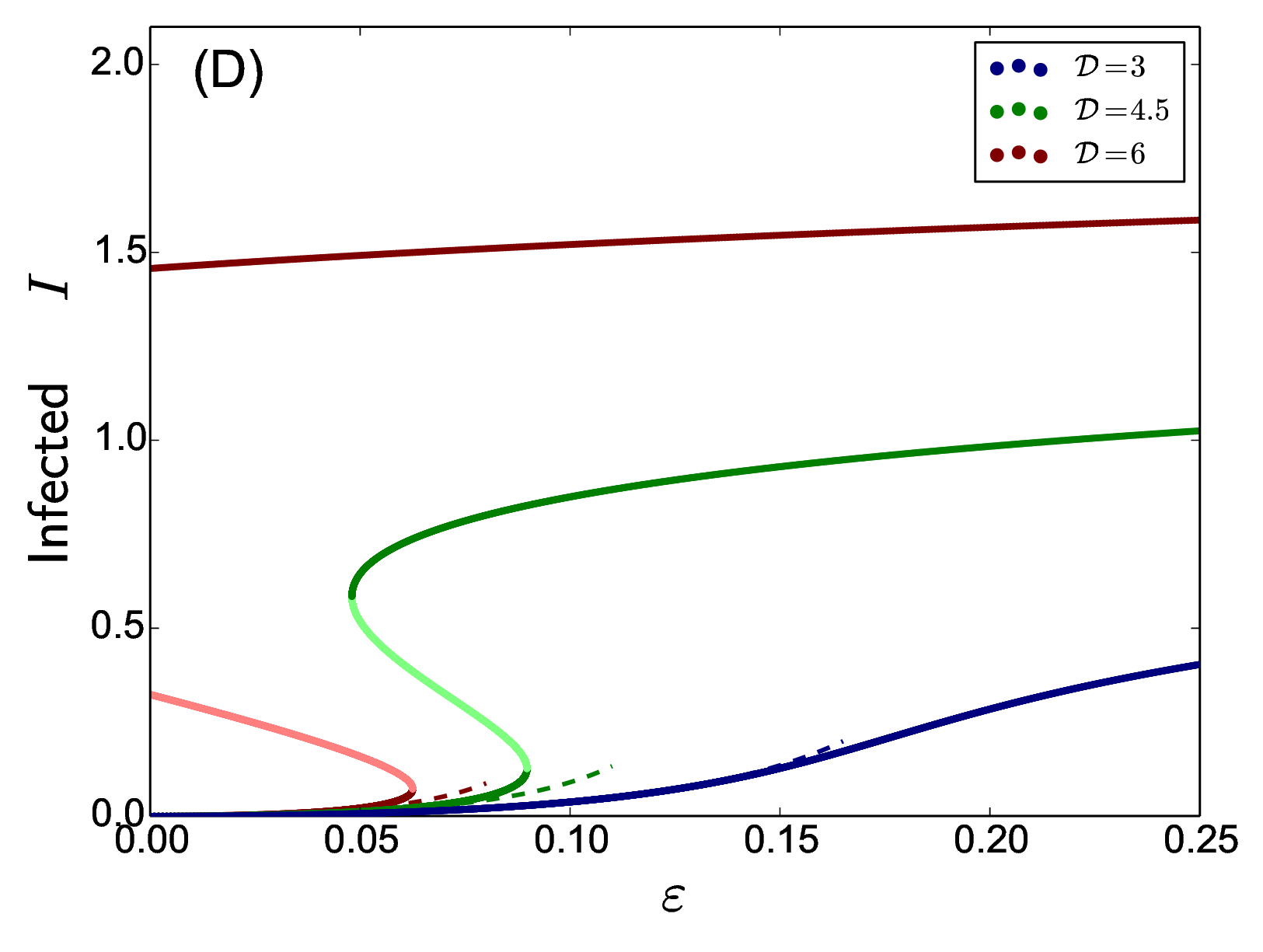
Figure 2: Equilibria of the vineyard model (4) as a function of $\epsilon$ for three different values of the vineyard density $\mathcal{D}$. Panels (A), (B), (C), (D) represent, respectively, the density of healty, full-grown plants (the $S$ compartment); healthy, young plants (the $G$ compartment); latent plants (the $L$ compartment); infected plants (the $I$ compartment). Dark/light color shades represent, respectively, stable and unstable equilibria. The dashed lines are the approximate expressions (16) of the equilibria close to the state (5) of healthy vineyard.

The system (3) may be brought to non-dimensional form by using $\tau$ as the scale of time and $(q\tau)^{-1/2}$ as the scale of grapevine density. Defining the non-dimensional quantities

$$(\tilde{S},\tilde{L},\tilde{I},\tilde{G})=(q\tau)^{1/2}(S,L,I,G),$$

the system in non-dimensional form reads:

$$\begin{cases}\dot{\tilde{S}}=&-\tilde{S}\left(\tilde{I}+\epsilon\right)^{2}+c_{1}\tilde{I}+c_{4}\tilde{G}\\ \dot{\tilde{L}}=&\hphantom{-}\tilde{S}\left(\tilde{I}+\epsilon\right)^{2}-c_{2}\tilde{L}\\ \dot{\tilde{I}}=&\hphantom{-}\tilde{G}\left(\tilde{I}+\epsilon\right)^{2}+c_{2}\tilde{L}-c_{1}\tilde{I}-c_{3}\tilde{I}\\ \dot{\tilde{G}}=&-\tilde{G}\left(\tilde{I}+\epsilon\right)^{2}-c_{4}\tilde{G}+\\ &\hphantom{-}\mathcal{D}-\left(\tilde{S}+\tilde{L}+\tilde{I}+\tilde{G}\right)\end{cases}$$ (4)

where the dot denotes derivation with respect to the non-dimensional time, and the (positive) constants are $c_{1}=k_{1}\tau$, $c_{2}=k_{2}\tau$, $c_{3}=k_{3}\tau$, $c_{4}=k_{4}\tau$, $\mathcal{D}=(q\tau)^{1/2}D$, $\epsilon=(q\tau)^{1/2}\varepsilon$. For typographical clarity for now on we shall omit the tildes have been omitted, and all quantities will be in non-dimensional form, unless otherwise specified.

2.2 Equilibria and their bifurcations

For initial data such that $S,L,I,G\geq 0$ and $S+L+I+G\leq\mathcal{D}$ then the solutions of (4) obey the bound $0\leq S,L,I,G\leq\mathcal{D}$ for all positive times (see Appendix 5.2 for a proof). If the initial condition is such that $S+L+I+G>\mathcal{D}$, then unacceptable solutions with negative values may develop. However, the only occurrence in which the density of the vineyard could be higher than the desired density $\mathcal{D}$ is when a farmer decides to thin out the vineyard in order to attain a lower desired density. Modeling this process is, of course, well beyond the aim of equations (4).

For $\epsilon=0$ the system (4) has the obvious equilibrium

$$S=\mathcal{D},\quad L=I=G=0$$ (5)

corresponding to an uninfected vineyard. Imposing the right-hand side of (4) to be zero, after some algebraic manipulations, the other equilibria of the model, for $I+\epsilon\neq 0$, may be expressed as solutions of the following system of non-linear algebraic equations:

$$\left\{\begin{array}[]{l}S={\displaystyle\frac{c_{1}I}{\left(I+\epsilon\right)^{2}}+{\displaystyle\frac{c_{3}c_{4}I}{\left(I+\epsilon\right)^{2}\left(c_{4}+\left(I+\epsilon\right)^{2}\right)}}}\\ L={\displaystyle\frac{c_{1}}{c_{2}}}I+{\displaystyle\frac{c_{3}c_{4}I}{c_{2}\left(c_{4}+\left(I+\epsilon\right)^{2}\right)}}\\ G={\displaystyle\frac{c_{3}I}{c_{4}+\left(I+\epsilon\right)^{2}}}\\ I=c_{3}^{-1}\left(\mathcal{D}-\left(S+L+I+G\right)\right)\end{array}.\right.$$ (6)

By substitution the first three equations of (6) into the fourth, one finds that the admissible equilibria (namely, those that do not have negative values in any of the four compartments) are determined by the non-negative roots of a fifth-order polynomial in the variable $I$. For $\epsilon=0$ one of the roots is $I=0$, which leads to the healthy vineyard equilibrium (5). For small values of $\epsilon$ there exists only one equilibrium at sufficiently small densities $\mathcal{D}$, and up to three at higher densities. No root exists with $I\geq\mathcal{D}$. Appendix 5.3 gives more details on these statements. The smallest positive root gives, for small non-zero $\epsilon$, an equilibrium very close to (5). A perturbative analysis confirms that very weak (or very far) hotbeds have almost no effect: if $\epsilon\ll 1$, then there exists an equilibrium which differs only by $O(\epsilon^{2})$ from the healthy vineyard. Explicit, approximate expressions of this equilibrium are given by eq. (16) in Appendix 5.4.

Families of equilibria depending on a parameter may be computed numerically [19, Chapter 10]. Using $\epsilon$ as the control parameter, the equilibria of the model (4) are shown in Figure 2, for several values of the vineyard’s desired density $\mathcal{D}$, and with $c_{1}=0.4$, $c_{2}=1/3$, $c_{3}=1$, $c_{4}=1/5$.

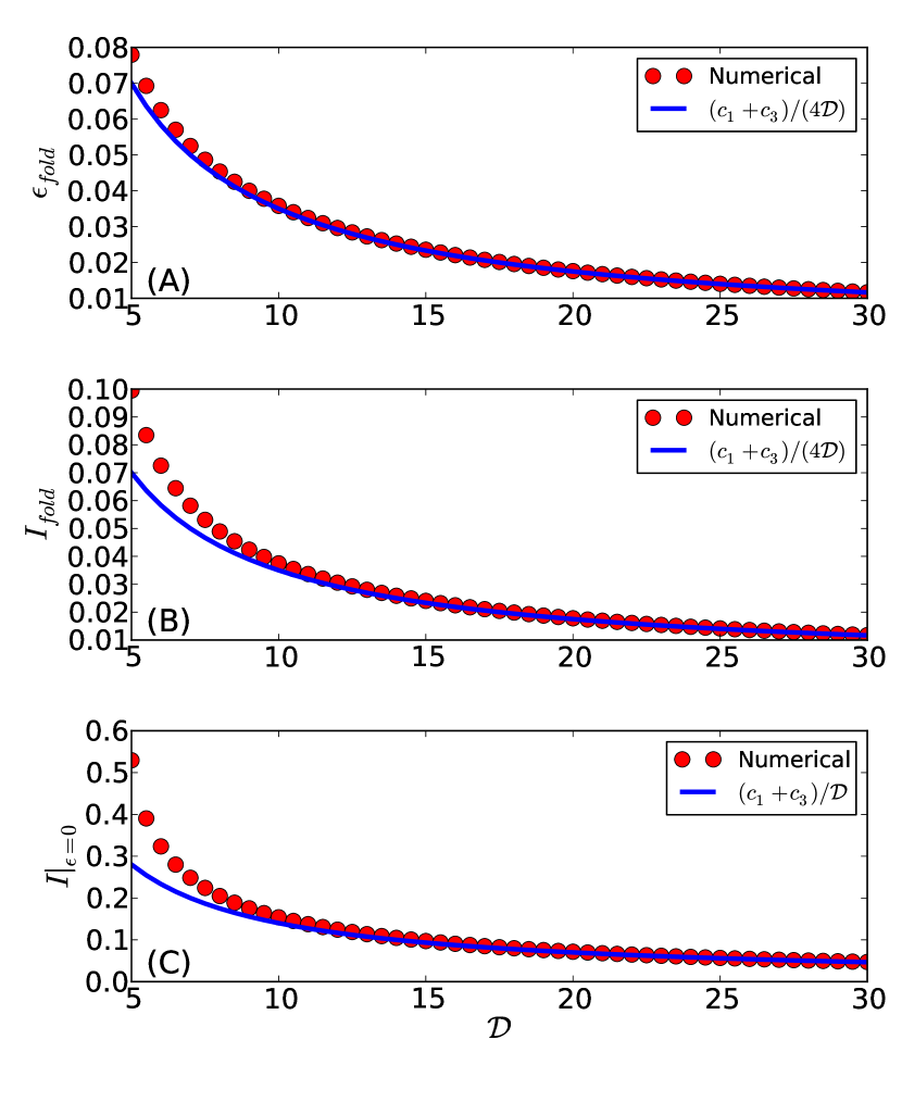
Figure 3: Panels (A) and (B): values of $\epsilon$ and of $I$ at the saddle-node bifurcation between the healthy vineyard branch and the saddle branch of equilibria for several values of $\mathcal{D}$. Panel (C): value of $I$ at the saddle equilibrium with $\epsilon=0$. The red dots are values computed numerically, the blue lines are the approximations discussed in the Appendix 5.5.

The linear stability of these equilibria is assessed by computing the eigenvalues of the linearization of equations (4) evaluated at the equilibrium. The healthy vineyard equilibrium (5) has four negative real eigenvalues $\lambda_{1,2,3,4}=(-1,-c_{1}-c_{3},-c_{2},-c_{4})$, and is therefore a stable node. For the other equilibria, shown in Figure 2, the eigenvalues were computed numerically. For $\mathcal{D}\lesssim 3.9$ there is only one equilibrium for each value of $\epsilon$, which is stable. At higher densities, there is an interval such that, if $\epsilon$ is within the interval, then there are three equilibria (two stable nodes and a saddle); if $\epsilon$ is outside the interval, then there is only one stable equilibrium; if $\epsilon$ is at one of the extremes of the interval, then the saddle and one of the two nodes coalesce in a saddle-node bifurcation (namely, the folds in Figure 2 where the curves have a vertical tangent and a stability change occurs). Only for intermediate values of the density $\mathcal{D}$ both extremes of this interval occur at positive values of $\epsilon$. For higher values of $\mathcal{D}$, the branch of stable equilibria that passes through the healthy vineyard equilibrium (5) folds at a positive $\epsilon$, the other stable branch folds at a negative $\epsilon$.

The critical values where the stable branch originating from the healthy vineyard state (5) looses stability have the following simple approximate expressions for large $\mathcal{D}$ (see Appendix 5.5 for details):

$$\epsilon_{fold}\approx\frac{c_{1}+c_{3}}{4\mathcal{D}},\qquad I_{fold}\approx\frac{c_{1}+c_{3}}{4\mathcal{D}}.$$ (7)

The critical values $S_{fold}$, $L_{fold}$, $G_{fold}$ are found by using (7) in (6). Figure 3 shows a comparison between the critical values determined numerically and the approximation (7).

2.3 The case of an abandoned vineyard

Sometimes, for economic reasons, vineyards are left unmanaged. In the absence of insecticide treatments and of active replacement of infected plants, unmanaged vineyards may become hotbeds of infection. A similar role is played by wild grapevines living in woodlands and shrublands. Equations (4) may be used to model these cases, simply by omitting the $G$ compartment of the young plants. The equations then read

$$\begin{cases}\dot{S}=&-SI^{2}+c_{1}I\\ \dot{L}=&\hphantom{-}SI^{2}-c_{2}L\\ \dot{I}=&-\left(c_{1}+c_{3}\right)I+c_{2}L\end{cases}$$ (8)

The values of the constants $c_{1}$ and $c_{2}$ may be taken the same as before. The mortality rate of the infected plants $c_{3}$ is, instead, much smaller, because plants are not actively eradicated once a year by a farmer, but rather die after several years of infection. We estimate that a single full-grown plant, when infected, should last about 10 years before dying (Table 1). In this very simplified approach we have omitted to introduce terms modeling the reproduction and the natural mortality of healthy grapevines. Owing to the long lifespan of grapevine plants, these processes occurs on time scales which are much longer than those involving the spread of FD, and should therefore be negligible in the present context. For simplicity, we have also omitted any coupling term with other nearby hotbeds: we assume that the abandoned vineyard is already infected, and we are interested in the time evolution of the most virulent phase of the infection, during which the abundance of infected individuals of S. titanus is determined by the local density of infected plants, and any inflow from external sources becomes negligible.

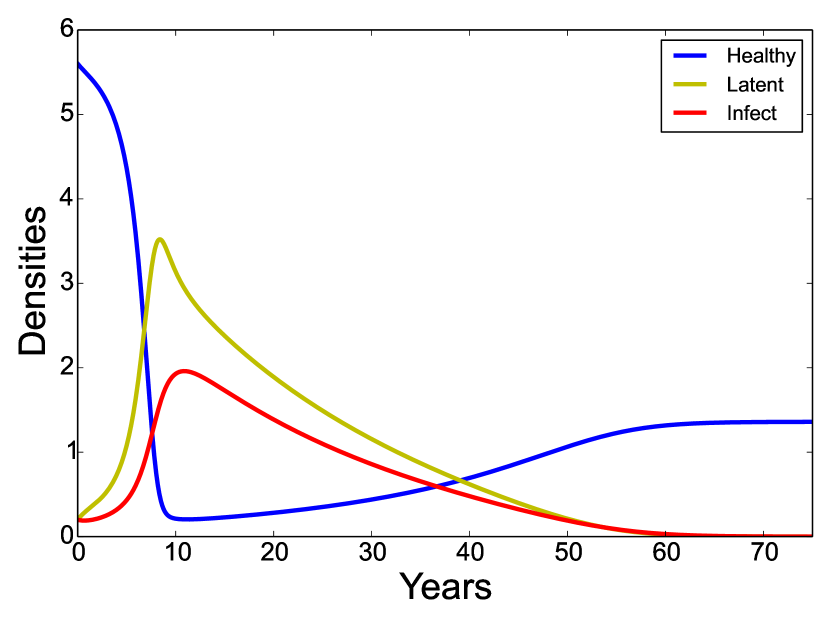
Figure 4: Numerical solution of equation (8) with the initial conditions $S(0)=5.6$, $L=0.2$, $I=0.2$. The constants $c_{1},$ $c_{2},$ $c_{3}$ are computed from the parameter values given in Table (1).

The set of states without infection $\mathcal{H}=\{S=S_{o},\,L=0,\,I=0\}$ where $S_{o}$ is an arbitrary constant, are the equilibria of the system of equations (8). By linearizing the equations around the equilibria we find that $\mathcal{H}$ is a normally hyperbolic manifold having two negative eigenvalues (namely, $\lambda_{1}=-c_{1}-c_{3}$ and $\lambda_{2}=-c2$). It is also the center manifold of each equilibrium [19, Chapter 5]. Therefore, initial conditions involving a very small number of infected and latent plants tend to fall back to an infection-free state in $\mathcal{H}$ without experiencing an appreciable growth of infected plants.

If the initial density of infected plants in the initial conditions is not very small, a more complicated dynamics, illustrated in Figure (4), will occur: from (8) we have

$$\frac{d}{dt}\left(L+I\right)=SI^{2}-\left(c_{1}+c_{3}\right)I,$$

thus, if initially it is $SI>c_{1}+c_{3}$, then the density of latent and infected plants will continue to grow as long as the latter inequality is satisfied. This produces, in the span of a few years, a dramatic decrease of the density of healthy plants mirrored by a corresponding rise of infected and latent plants. As the number of infected plants increases, so does the number of plants that recover and become healthy again. The epidemic peaks when the recovered plants become a substantial fraction of the healthy plants. This is in qualitative agreement with the results of the experiments of Morone et al. [3]. After this rapid, virulent phase, the density of healthy plants has dropped so much that $SI<c_{1}+c_{3}$. The density of latent and infected plants slowly decreases, whereas the density of healthy plants experiences a slow growth, thanks to the recovery of previously infected plants. Eventually, after an almost century-long transient, the abandoned vineyard returns to a healthy state, but with a drastically lower plant density.

3 Discussion

3.1 Practical implications of the structure of the bifurcation diagram

The bifurcation analysis of Section 2.2 shows the crucial importance of infection hotbeds in determining the state of a nearby vineyard. If the hotbeds are absent or weak (that is, if the value of $\epsilon$ is small), then there is always a stable state which doesn’t differ much from the healthy vineyard state: infected plants are very few and replacing them with young ones keeps the infection at very low levels.

If $\epsilon$ increases, the outcome depends on the value of the parameter $\mathcal{D}$ (the non-dimensional design density of the vineyard). For densities $\mathcal{D}\lesssim 3.9$ (which, according to our estimate of $q$, correspond to $D\lesssim 3900\;\mathrm{plants\,ha^{-1}}$) the number of healthy plants decreases gradually with increasing $\epsilon$: one would observe a progressive worsening of the vineyard’s health as the hotbeds become stronger (see the blue curve in Figure 2). For higher densities, the gradual decrease occurs only up to the critical value $\epsilon_{fold}$. When the strength of the hotbeds becomes such that $\epsilon>\epsilon_{fold}$, then the stable fixed point, corresponding to a vineyard with just a few infected plants, disappears. As a consequence, the vineyard undergoes a transition towards the only stable fixed point left, corresponding to a state dominated by infected and latent plants.

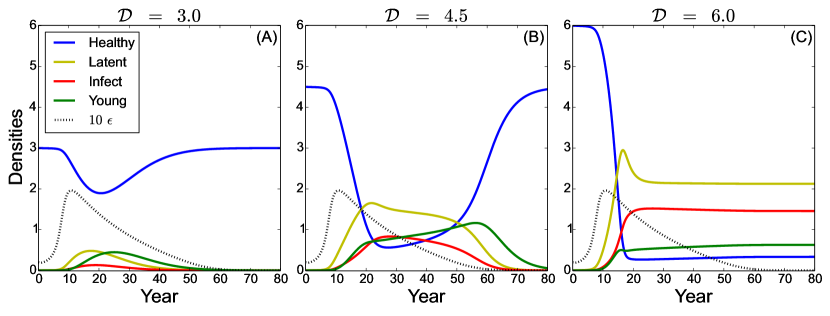
Figure 5: Time evolution of of a vineyard with design density $\mathcal{D}=3$ (A), $\mathcal{D}=4.5$ (B), and $D=6$ (C) exposed to hotbeds with a time-varying strength $\epsilon$. Note that, for clarity, the value of $\epsilon$ (represented by the dotted black line) is multiplied by ten.

After the transition, if the strength of the hotbeds eventually decreases and returns to zero, the outcome also depends on the design density of the vineyard. If $\mathcal{D}\lesssim 4.8$ (corresponding to $D\lesssim 4800\;\mathrm{plants\,ha^{-1}}$) then there exists another critical value of $\epsilon$, such that, when the strength of the hotbeds is lower than this critical value, the system experiences a transition back to the state with just a few infected plants (see the green curves in Figure 2). In this case, one would observe a classic hysteresis cycle. For higher densities (see the red curves in Figure 2) performing a complete cycle is impossible: the second critical value of $\epsilon$ is negative, which is impossible to attain, because it would correspond to a meaningless negative density of infected plants in the hotbeds. Therefore, even if all the hotbeds were removed (that is, $\epsilon=0$) the vineyard would remain stuck in the stable state with very few healthy plants.

In order to further elucidate this dynamics, and to show how the structure of the bifurcation diagram shapes the time evolution of a vineyard exposed to a nearby hotbed, we have solved numerically the equations (4) with a time varying $\epsilon$. We have set $\epsilon=c_{o}I_{a}$, where $I_{a}$ is the density of infected plants in an abandoned vineyard according to the model (8), with the parameters and initial conditions of Figure 4. The strength of the hotbed peaks about ten years after the beginning of the simulation, then slowly returns to zero. By setting $c_{o}=0.1$, and keeping all the other parameters of the managed vineyard as in Figure 2, we obtain the results shown in Figure 5.

At low densities (Figure 5 A) there is only one stable fixed point for each value of $\epsilon$. Thus, as $\epsilon$ varies in time, the state of the vineyard changes gradually, with only a moderate loss of healthy plants. When $\epsilon$ returns to zero, the vineyard returns to a healthy state.

At intermediate densities (Figure 5 B), after the initial transient during which the number of healthy plants decreases very slowly, the strength of the hotbed crosses the bifurcation point. The vineyard then experiences a rapid transition to the state with very few healthy plants. When the strength of the hotbed decreases below the second critical value, then the vineyard slowly recovers, and returns to a healthy state, closing the hysteresis cycle.

At high densities (Figure 5 C), there is also a rapid transient to the state with few healthy plants, but then the vineyard never recovers the healthy state, even for vanishingly low strengths of the hotbed, because the second critical point is unreachable and the hysteresis loop can not be closed.

3.2 The effect of the insecticides

Because insecticides cause a drop in the number of adults of S. titanus, they diminish the strength of the coupling between the infected and the healthy plants. In our model this translates in a decrease of the value of the parameter $q$ which appears in equations (3).

The consequences of this decrease are best understood by recalling that $q$ appears in the scale of density used to define the non-dimensional compartments. In particular, the non-dimensional design density and the dimensional one, are linked by the following identity

$$\mathcal{D}=\left(q\tau\right)^{1/2}D.$$ (9)

It follows that a decrease in $q$ is equivalent to a decrease in the non-dimensional value of the vineyard’s design density $\mathcal{D}$. Thus, the persistent use of insecticides may have the effect of changing the shape of the bifurcation diagram of a given vineyard from, say, one that looks like the red curves in Figure (2) to one that looks like the blue curves.

In this respect, insecticides should be seen as beneficial, because, by potentially removing the fold bifurcations, they avoid catastrophic transitions from a state in which the vineyard is close to the healthy state, to one in which most of the plants are either infected or latent. However, the insecticide treatment can not be interrupted while there are still nearby hotbeds of infection, because the bifurcation diagram would spring back to its original shape, and the state of the vineyard would rapidly deteriorate, even if it had attained an almost perfect recovery during the years of insecticide treatment.

On the other hand, if the hotbeds of infection were gradually eliminated, any vineyard still in relatively good health would return to the healthy state, without the need of insecticides, thanks just to the continued action of extirpation of the infected plants and replacement with the young ones. Therefore, the elimination of hotbeds as a source of inoculum seems to be crucial in maintaining a healthy status in vineyards.

In the situations in which a decrease of the value of $\mathcal{D}$ is desirable, this can also be achieved by decreasing the design density $D$ of the vineyard. In order to do so, a farmer may replace with young plants only a fraction of those eradicated because infected. This procedure has the added benefit of reducing the number of young plants in the vineyard, which, being not subject to a latency period, may immediately become infected, thus helping spreading the disease. Obviously, the decision of decreasing the design density of a vineyard has to be evaluated also on the basis of economic considerations, but it seems unwise to unconditionally exclude this option, and rely exclusively on insecticide treatments.

3.3 The functional form of the infection rate

We have argued that the function $f$ appearing in the infection rate (1) should grow faster than linearly with $I$ at low numbers of infected plants. In order to support our argument we have also investigated the case in which the infection rate is

$$\mathrm{Infection\,\,rate}=\hat{q}SI$$ (10)

where $\hat{q}$ is expressed as $\mathrm{ha\,plants^{-1}Y^{-1}}$. Thus a scale of grapevine density is $(\hat{q}\tau)^{-1}$. Using (10) in place of (2), the non-dimensional model (4) becomes the following

$$\begin{cases}\dot{S}=&-S\left(I+\hat{\epsilon}\right)+c_{1}I+c_{4}G\\ \dot{L}=&\hphantom{-}S\left(I+\hat{\epsilon}\right)-c_{2}L\\ \dot{I}=&\hphantom{-}G\left(I+\hat{\epsilon}\right)+c_{2}L-c_{1}I-c_{3}I\\ \dot{G}=&-G\left(I+\hat{\epsilon}\right)-c_{4}G+\\ &\hphantom{-}\hat{\mathcal{D}}-\left(S+L+I+G\right)\end{cases}$$ (11)

where $\left(\hat{\mathcal{D}},\hat{\epsilon}\right)=\hat{q}\tau\left(D,\varepsilon\right)$. The state of healthy vineyard (5) is obviously an equilibrium also for equations (11). A linear stability analysis shows that the linearization around this equilibrium has three negative eigenvalues. The fourth eigenvalue is

$$\lambda_{4}=\frac{\sqrt{4c_{2}\left(\mathcal{D}-c_{1}-c_{3}\right)+\left(c_{1}+c_{2}+c_{3}\right)^{2}}-\left(c_{1}+c_{2}+c_{3}\right)}{2}.$$

The healthy vineyard is the unstable if $\lambda_{4}>0$, that is if

$$\mathcal{D}>c_{1}+c_{3}.$$ (12)

A bifurcation analysis analogous to that of Section 2.2 shows that the state of healthy vineyard is part of a family of equilibria which exists for any $\epsilon\geq 0$ and is not subject to any bifurcation.

When (12) is satisfied, this family of equilibria is unstable. In addition, the $G$ compartment assumes negative values for $\epsilon>0$, which makes these equilibria ecologically meaningless. For the same parameters, there is a second family of equilibria which is stable, ecologically acceptable, and corresponds to a vineyard dominated by infected and latent plants.

If (12) is not satisfied, and $\mathcal{D}<c_{1}+c_{3}$ holds, then the family of equilibria containing the healthy vineyard is stable, and no compartment assumes negative values for any value of $\epsilon$. For increasing $\epsilon$, the density of healthy plants gradually decreases and that of latent and infected plants gradually increases.

An analysis analogous to that reported in Section 5.1 leads to an estimate of $\hat{q}$ in the range $10^{-3}$ to $10^{-2}$ $\mathrm{ha\,plants^{-1}Y^{-1}}$. Estimating $c_{1}+c_{3}\approx 1.4$ (see Table 1), this suggests that the typical healthy vineyard should be unstable to infinitesimal perturbations. As a consequence, even a small number of infected adults of S. titanus would precipitate a healthy vineyard into the stable state dominated by infected plants, on a time scale proportional to $\lambda_{4}^{-1}$. If, on the other hand, $\hat{q}$ were as small as to make stable the state of healthy vineyard, then a vineyard would never become dominated by infected plants, except when surrounded by very strong and virulent hotbeds.

Table 2: For seven Italian regions we report the date of the first known appearence of Flavescence Dorée, and the date of the beginning of the epidemics. In the region Marche, as of today, three well-established hotbeds have been reported, but not a widespread epidemics. For Valle d’Aosta the beginning of the epidemics is estimated from personal communications.

Region	First known appearence	Beginning of the epidemics
Veneto	1976 [21]	1980-82 [27]
Trentino	1985 [22]	1992 [28]
Friuli	uncertain	1986 [25]
Marche	2001 [26]	not yet [30]
Piemonte	1978 [23]	1998 [3]
Valle d’Aosta	2006 [24]	2010
Lombardia	1972 [20]	1985 [29]

These findings are at odds with the observed phenomenology of infestations of FD. If the model (11) were correct, when exposed to FD, a well-managed vineyard would either develop just a small number of infected plants, without further progresses (stable healthy state), or, more likely, rapidly experience a destructive infestation (unstable healthy state). A transition from the first to the second situation (as shown in Figure 5 B, C) appears to be impossible if one accepts the expression (10) for the infection rate. An example of this transition is reported for Serbia, where several vineyards of cultivar “Plovdina”, very sensitive to FD, raised up to a 100% symptomatic grapes in three years starting from an infection rate lower than 5% [31].

Table 2 shows that, in Italian wine-making regions, there has always been a delay of several years from the date of the first report of FD, to the date of the beginning of the epidemic status. The latter may be defined as when FD starts to spread all over the territory without being confined to a few hot points. Generally, the epidemic status is recognized when a consistent part of the vineyards has more than 30% of infected plants, and eradication is not considered possible anymore. For instance, in Piedmont, the territory is classified as: free but vulnerable areas (FD absent, but very likely to occur); hotspot areas (FD present but not settled, possible to eradicate); settlement areas (FD settled, impossible to eradicate).

If healthy vineyards were unstable with respect to small inflows of infected adults of S. titanus, one would expect a much more rapid development of the epidemics. The observed slow progression of the infestation, together with the fact that, in the presence of an epidemics, the infestation in a vineyard is unlikely to remain limited to a small portion of the plants, but generally progresses up to a state dominated by infected plants (sometimes even if insecticides are used), strongly points to the existence of a critical transition between two alternative stable states of almost-healthy vineyard and completely infested vineyard, as suggested by the bifurcation diagram of Figure 2.

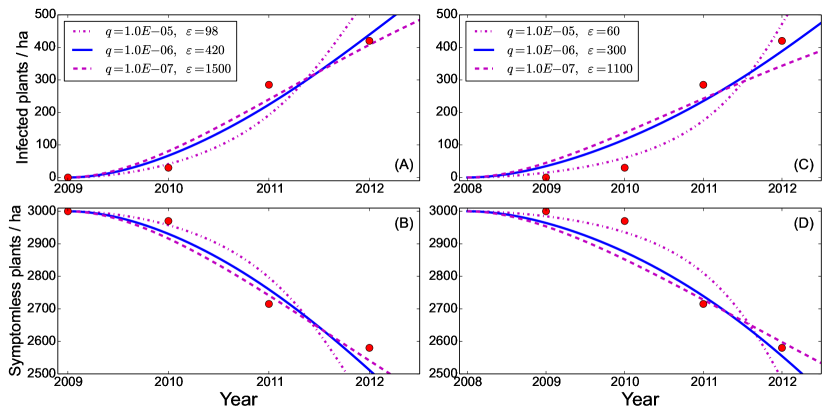
Figure 6: Comparison between observed data (dots) and the model (lines) for different values of the parameter $q$. In panels (A), (C) the dots represent the observed density of infected plants in an experimental vineyard, the lines are the $I$ compartment. In panels (B), (D) the dots represent the observed density of symptomless plants, the lines are the sum of the $S$ and $L$ compartments. In panels (A), (B) the numerical solution starts in 2009, and uses the $q\;\left(\mathrm{ha^{2}plants^{-2}Y^{-1}}\right)$ and $\varepsilon\;\left(\mathrm{plants\,ha^{-1}}\right)$ values given in the inset of panel (A). In panels (C), (D) the solution starts in 2008 and the $q,\;\varepsilon$ values are given in the inset of panel (C).

4 Conclusions

We have developed a model for the time evolution of a FD epidemics in a vineyard. The presence of the vector of the disease (the leafhopper Scaphoideus titanus Ball) is not explicitly modeled, but is parameterized as an interaction term between the infected and the healthy grapevine plants. The presence of infection hotbeds near the vineyard appears as a parameter in this interaction term. In addition to infection, the model takes also into account incubation, recovery and aging processes, and also extirpation and replacement of infected plants, operated by the farmer.

The model shows that, in the presence of abundant populations of S. titanus, or, equivalently, for vineyards with high plant density, two stable equilibria are possible. One of these corresponds to a situation with just a few infected plants, where the infection is kept under control by the extirpation and replacement process. The other equilibrium corresponds to a vineyard dominated by infected plants, where extirpation and replacement is ineffective. When the strength of the hotbeds crosses a critical threshold, only the latter equilibrium survives, and the former disappears. Therefore, vineyards infected with FD may undergo an irreversible transition from a near-healthy state to a severely compromised one.

The model suggests that insecticide treatments, together with continued extirpation and replacement of infected plants, may be an effective way to recover from a severe infestation. However, the model also demonstrates that insecticides are just a stopgap measure. Without the elimination of the hotbeds, FD would not disappear from an infested vineyard, and any weakening of the treatments may precipitate the situation again. This finding calls for a proactive search and removal of any infection hotbeds as soon as the presence of FD becomes apparent in a grapevine-farming territory. These preventive measures, if successful, could avoid the need of extensive insecticide treatments on productive vineyards.

Acknowledgements

This research was conducted within the frame of the project: "Elaborazione e stesura di un protocollo di lotta guidata alla Flavescenza dorata e al suo vettore Scaphoideus titanus nella zona di produzione dell’Asti docg", funded by "Consorzio per la tutela dell’Asti docg". We thank Jost von Hardenberg for a helpful discussion on this problem.

5 Appendix

5.1 An estimate of the value of $q$

As part of an experiment in the province of Cuneo (Italy), a small vineyard of $0.475$ ha was monitored from 2009 to 2012. The vineyard had an initial density $D=3000$ plants/ha and no infected plants. Flavescence Dorée was already well established in the surrounding territory. However we lack quantitative data allowing for the estimation of the appropriate value of $\varepsilon$. No insecticide treatments, nor extirpation of infected plants was performed. Every year, the number of infected and simptomless plants was assessed (the red dots in Figure 6 (A), (C) and (B),(D), respectively). The assessment would not distinguish between healthy and latent plants, both classified as symptomless.

In order to determine a reasonable range of values of $q$, we apply the model (3) by setting $G=0$ and dropping the last equation (which models the replacement of infected plants with young ones). Figure (6) shows a comparison between the model results and the observed data, for several choices of the parameters $q$ and $\varepsilon$. The other coefficients are those of Table 1. The density of symptomless plants is compared with the sum of the $S$ and $L$ compartments. The initial condition is $S=D$, $L=I=0$. In Figures 6 (A), (B) the numerical solution starts in 2009, the last year without infected plants. In Figures 6 (C), (D) the solution starts in 2008. This allows for the hypothesis that for one year all the inoculated plants remained in the latent state, or with symptoms as weak as to evade detection. In the first case, $q\approx 10^{-6}\,\mathrm{ha^{2}plants{}^{-2}\,Y^{-1}}$ gives a reasonable fit of the data, while in the second a value as high as $q\approx 10^{-5}\,\mathrm{ha^{2}plants{}^{-2}\,Y^{-1}}$ yields a more convincing fit. Values as low as $q\approx 10^{-7}\,\mathrm{ha^{2}plants{}^{-2}\,Y^{-1}}$ also give an acceptable fit, if the initial condition refers to 2009, but should probably be ruled out, because they require unrealistically high values of $\varepsilon$.

5.2 Boundedness and non-negativity of the solutions

For non-negative initial conditions such that $S+L+I+G\leq\mathcal{D}$ the solutions of the model equations (4) remain non-negative and bounded by $\mathcal{D}$ at all later times. In fact, by adding together the four equations in (4), and defining the total vineyard density $x=S+L+I+G$, we obtain

$$\dot{x}=\mathcal{D}-x-c_{3}I.$$ (13)

Considering $I$ as a known function of time, we have that the solution of (13) is

$$x(t)=\mathcal{D}+\left(x(0)-\mathcal{D}-c_{3}\int_{0}^{t}e^{s}I(s)\,\mathrm{d}s\right)e^{-t}.$$ (14)

This shows that, if the initial vineyard density is $x(0)\leq\mathcal{D}$, then, as long as $I$ remains non-negative, it will be $x(t)\leq\mathcal{D}$. But if at any time $t$ we have $S,L,I,G\geq 0$ and $x(t)\leq\mathcal{D}$, then from (4) we deduce $S=0\Rightarrow\dot{S}\geq 0$, $L=0\Rightarrow\dot{L}\geq 0$, $I=0\Rightarrow\dot{I}\geq 0$, and $G=0\Rightarrow\dot{G}\geq 0$. Therefore, none of the four compartments can become negative. Thus we have that $0\leq x(t)\leq\mathcal{D}$ at all times, which implies $0\leq S,L,I,G\leq\mathcal{D}$.

5.3 Determination of the equilibria of the model

By substituting the first three expressions of (6) in the fourth, and then multiplying by $c_{2}\left(I+\epsilon\right)^{2}\left(\left(I+\epsilon\right)^{2}+c_{4}\right)$ we obtain that the equilibrium densities of infected plants are the non-negative roots of the fifth-order polynomial $\mathcal{P}(I)=\sum_{n=0}^{5}q_{n}I^{n}$, whose coefficients are

$$\begin{array}[]{l}q_{5}=\hphantom{-}c_{2}\left(c_{3}+1\right)+c_{1}\\ q_{4}=-c_{2}\mathcal{D}+4q_{5}\epsilon\\ q_{3}=\hphantom{-}c_{2}\left(c_{3}+1\right)c_{4}+\left(c_{1}+c_{3}\right)\left(c_{2}+c_{4}\right)+4q_{4}\epsilon-10q_{5}\epsilon^{2}\\ q_{2}=-c_{2}c_{4}\mathcal{D}+2q_{3}\epsilon-2q_{4}\epsilon^{2}\\ q_{1}=\hphantom{-}c_{2}\left(c_{3}+c_{1}\right)c_{4}+2q_{2}\epsilon-3q_{3}\epsilon^{2}+4q_{4}\epsilon^{3}-5q_{5}\epsilon^{4}\\ q_{0}=-c_{2}c_{4}\mathcal{D}\epsilon^{2}-c_{2}\mathcal{D}\epsilon^{4}\end{array}$$ (15)

Recalling that $c_{1},\ldots,c_{4}>0$ and $\mathcal{D}>0$, from the last equation in (3) it follows that there are no equilibria with $I\geq\mathcal{D}$ and $S,L,G\geq 0$. Because from (6) it follows that to any non-negative root of $\mathcal{P}$ corresponds an equilibrium with non-negative values for all the four compartments, then we deduce that $\mathcal{P}$ cannot have real roots larger than $\mathcal{D}$.

Note that the coefficients $q_{5},\ldots,q_{0}$ are polynomials in $\epsilon$. We observe that, for any given $\mathcal{D}$, there are sufficiently small values of $\epsilon$ so that the coefficients of the odd powers are positive and those of the even powers are negative. Then, from Descartes’ rule of signs, it follows that $\mathcal{P}$ has no negative roots. Hence, being an odd-degree polynomial, it must have at least one non-negative real root. In the special case $\epsilon=0$ then $q_{0}=0$, and a real root is $I=0$, which yields the equilibrium (5). We also observe that for any positive value of $\epsilon$ as small as to make $q_{3},q_{1}>0$, $2q_{3}>q_{4}\epsilon$, there exist sufficiently small values of $\mathcal{D}$ such that $q_{4},q_{2}>0$. Then, from Descartes’ rule of signs, it follows that $\mathcal{P}$ has one, and only one positive root.

An extensive numerical exploration for reasonable values of the parameters has never yielded more than three positive real roots for $\mathcal{P}$. Neither we found numerical evidence of limit cycles or deterministic chaos. We therefore are confident that the bifurcation diagrams shown in Figure 2 determine all the qualitative dynamics of the model equations (4).

5.4 Approximate explicit expressions for the equilibria near the state of healthy vineyard

For $\epsilon\ll 1$, explicit, approximate expressions for the equilibria of the model (4) may be sought perturbatively, assuming an expansion of the form

$$S(\epsilon) = \mathcal{D}+\epsilon S_{1}+\epsilon^{2}S_{2}+\epsilon^{3}S_{3}+\cdots$$

$$L(\epsilon) = \epsilon L_{1}+\epsilon^{2}L_{2}+\epsilon^{3}L_{3}+\cdots$$

$$I(\epsilon) = \epsilon I_{1}+\epsilon^{2}I_{2}+\epsilon^{3}I_{3}+\cdots$$

$$G(\epsilon) = \epsilon G_{1}+\epsilon^{2}G_{2}+\epsilon^{3}G_{3}+\cdots$$

which represents a small correction upon the healthy vineyard equilibrium. The perturbative analysis reveals that $S_{1}=L_{1}=I_{1}=G_{1}=0$. That is, weak hotbeds at first perturbative order have no effect on a healthy vineyard. The second and higher orders are non-zero, and the information that they carry is best conveyed by using Padé approximants. The (2,1) Padé approximation of the equilibrium computed with the perturbative expansion up to the third order is the following

$$\begin{array}[]{l}S(\epsilon)=\mathcal{D}-{\displaystyle\frac{\left(c_{2}c_{3}+c_{4}\left(c_{1}+c_{2}+c_{3}\left(c_{2}+1\right)\right)\right)}{c_{2}c_{4}\left(c_{1}+c_{3}-2\epsilon\mathcal{D}\right)}}\epsilon^{2}\\ L(\epsilon)={\displaystyle\frac{\left(c_{1}+c_{3}\right)\mathcal{D}}{c_{2}\left(c_{1}+c_{3}-2\epsilon\mathcal{D}\right)}}\epsilon^{2}\\ I(\epsilon)\,={\displaystyle\frac{\mathcal{D}}{\left(c_{1}+c_{3}-2\epsilon\mathcal{D}\right)}}\epsilon^{2}\\ G(\epsilon)={\displaystyle\frac{c_{3}\mathcal{D}}{c_{4}\left(c_{1}+c_{3}-2\epsilon\mathcal{D}\right)}}\epsilon^{2}\end{array}$$ (16)

5.5 Approximate position of the saddle-node bifurcation

If the vineyard’s desired density $\mathcal{D}$ is sufficiently high, for $\epsilon=0$ there are three equilibria: the healthy vineyard stable node (5) (with no infected plants), a saddle (with an intermediate number of infected plants), and another stable node (with a high number of infected plants). As the parameter $\epsilon$ grows, the branch of stable nodes which passes through (5) and the branch of saddles move close to each other, and meet in a saddle-node bifurcation at $\epsilon_{fold}$ (e.g. Figure 2(D) for $\mathcal{D}=6$). The value of $\epsilon_{fold}$ and of the corresponding equilibrium value of infected plants $I_{fold}$ may be approximated with explicit expressions, as shown in Figure 3.

First we observe that for positive $\epsilon$ and sufficiently large $\mathcal{D}$ the polynomial $\mathcal{P}$ has one real positive root of size $O(\mathcal{D})$. The other roots, as $\mathcal{D}\to\infty$, tend to the solutions of

$$I^{4}+c_{4}I^{2}+c_{4}\epsilon^{2}+\epsilon^{4}=0$$

(where we have used the expressions (15) divided by $\mathcal{D}$). But this polynomial does not have real solutions. Therefore we conclude that for fixed $\epsilon>0$ and asymptotically large $\mathcal{D}$, the polynomial $\mathcal{P}$ has only one real root, which is positive.

For $\epsilon=0$ the polynomial $\mathcal{P}$ has the root $I=0$. The other equilibria are given by the solutions of

$$\frac{q_{5}}{\mathcal{D}}I^{4}-c_{2}I^{3}+\frac{q_{3}}{\mathcal{D}}I^{2}-c_{2}c_{4}I+\frac{c_{2}c_{4}\left(c_{1}+c_{3}\right)}{\mathcal{D}}=0$$ (17)

where $q_{5},q_{3},q_{1}$ are given by (15) with $\epsilon=0$. For $\mathcal{D}\to\infty$ one of the solutions of (17) approaches zero. Therefore it may be approximated by neglecting the terms of order higher than the first, yielding

$$\left.I\right|_{\epsilon=0}\approx\frac{c_{1}+c_{3}}{\mathcal{D}}.$$ (18)

For $0\leq\epsilon\leq\epsilon_{fold}$, a smooth family of equilibria connects the equilibrium corresponding to (18) to the healthy vineyard equilibrium (5), changing stability at $\epsilon_{fold}$. But for $\mathcal{D}\to\infty$ it must be $\epsilon_{fold}\to 0$ because for large $\mathcal{D}$ and positive $\epsilon$, $\mathcal{P}$ has only one real solution. Thus, if the family of equilibria is a smooth curve, asymptotically for large $\mathcal{D}$, it must be $0<I_{fold}<\left.I\right|_{\epsilon=0}$ and $\epsilon_{fold}\propto I_{fold}$. We have verified numerically for a large number of values of $c_{1},$ $c_{3}$ and $\mathcal{D}$, that

$$I_{fold}=\epsilon_{fold}=\frac{\left.I\right|_{\epsilon=0}}{4}$$

is a very good approximation for the position of the saddle-node bifurcation, except for the values of $\mathcal{D}$ so low that for $\epsilon=0$ , $\mathcal{P}$ has only the real root $I=0$ (e.g. the case $\mathcal{D}=4.5$ in Figure 2(D)).

References

- [1] Malembic-Maher S., Salar P., Carle P. and Foissac X., 2009. Ecology and taxonomy of Flavescence dorée phytoplasmas: the contribution of genetic diversity studies. Progrès Agricole et Viticole, 2009, Hors Série-Extended abstracts 16th meeting of ICVG, Dijon, France, 31 Aug.-4 Sept. 2009, pp. 132-134.
- [2] Osler R., Zucchetto C., Carraro L., Frausin C., Pavan F., Vettorello G., Girolami V., 2002. Trasmissione di flavescenza dorata e legno nero e comportamento delle viti infette. L’Informatore Agrario 19: 61-65.
- [3] Morone C., Boveri M., Giosuè S., Gotta P., Scapin I., Marzachì C., 2007. Epidemiology of Flavescence dorée in vineyards in Nortwestern Italy. Phytopathology 97: 1422-1427.
- [4] Bonfils J., Schvester D., 1960. Les Cicadelles (Homoptera Auchenorrhyncha) dans leur rapports avec la vigne dans le sud-ouest de la France. Annales Epiphyties 11: 325-336.
- [5] Vidano C., 1964. Scoperta in Italia dello Scaphoideus littoralis Ball cicalina americana collegata alla “Flavescence dorée” della vite. L’Italia Agricola 101: 1031-1049.
- [6] Bressan A., Larrue J., Boudon-Padieu E., 2006. Patterns of phytoplasma-infected and infective Scaphoideus titanus leafhoppers in vineyards with high incidence of Flavescence dorée. Entomologia Experimentalis et Applicata 119: 61-69.
- [7] Bressan A., Spiazzi S., Girolami V., Boudon-Padieu E. 2005. Acquisition efficiency of Flavescence dorée phytoplasma by Scaphoideus titanus Ball from infected tolerant of susceptible grapevine cultivars or experimental host plants. Vitis 44: 143-146.
- [8] Alma A., Bosco D., Danielli A., Bertaccini A., Vibio A., Arzone A., 1997. Identification of phytoplasmas in eggs, nymphs and adults of Scaphoideus titanus Ball reared on healthy plants. Insect Molecular Biology 6: 115-121.
- [9] Filippin L., Jovic J., Cvrkovic T., Forte V., Clair D., Tosevski I., Boudon-Padieu E., Borgo M., Angelini E., 2009. Molecular characteristics of phytoplasmas associated with Flavescence dorée in clematis and grapevine and preliminary results on the role of Dictyophara europaea as a vector. Plant Pathology 58: 826-837.
- [10] Zorloni A., Casati P., Quaglino F., Bulgari D., Bianco P.A., 2008. Incidenza del fenomeno del “recovery” in vigneti della Lombardia. Petria 18: 388-390.
- [11] Galetto L., Roggia C., Marzachi C., Alma A., Bosco D., 2009. Acquisition of Flavescence dorée phytoplasma by Scaphoideus titanus from recovered and infected grapevines of Barbera and Nebbiolo cultivars. Progrès Agricole et Viticole, 2009, Hors Série-Extended abstracts 16th meeting of ICVG, Dijon, France, 31 Aug.-4 Sept. 2009, pp. 170-171.
- [12] Pavan F., Mori N., Bigot G., Zandigiacomo P., 2012. Border effect in spatial distribution of Flavescence dorée affected grapevines and outside source of Scaphoideus titanus vectors. Bulletin of Insectology 65 (2): 281-290.
- [13] Lessio F. Tota F., Alma A. Tracking the dispersal of Scaphoideus titanus Ball from wild to cultivated grapes: use of a novel mark-capture technique. Bulletin of Entomological Research. DOI 10.1017/S0007485314000030.
- [14] Maggi F., Marzachì C., Bosco D., 2013. A Stage-Structured Model of Scaphoideus titanus in Vineyards. Environmental Entomology, 42 (2): 181-193.
- [15] Lessio F., Albertin I., Lombardo D.M., Gotta P., Alma A., 2011a. Monitoring Scaphoideus titanus for IPM purposes: results of a pilot-project in Piedmont (NW Italy). Bulletin of Insectology 64: 269-270.
- [16] Lessio F., Borgogno Mondino E., Alma A., 2011b. Spatial patterns of Scaphoideus titanus (Hemiptera: Cicadellidae): a geostatistical and neural network approach. International Journal of Pest Management 3: 205-216.
- [17] Chuche J., Thiéry D., 2014. Biology and ecology of the Flavescence dorée vector Scaphoideus titanus: a review. Agronomy for Sustainable Development. DOI 10.1007/s13593-014-0208-7.
- [18] Schvester D., Carle P., Moutous G., 1969. Nouvelles données sur la transmission de la Flavescence dorée de la vigne par Scaphoideus littoralis Ball. Annales de Zoologie et Écologie Animal 1(4): 445-465.
- [19] Y. A. Kuznetsov, 1995. Elements of applied bifurcation theory. Applied Mathematcal Sciences, 112, II edition. Springer-Verlag, New York.
- [20] Belli G., Fortusini A., Osler R., Amici A., 1973. Presenza di una malattia del tipo "flavescence dorée" in vigneti dell’Oltrepò pavese. Rivista di Patologia Vegetale 9(suppl.): 50-56.
- [21] Egger E., Borgo M., 1983. Diffusione di una malattia virus-simile su "Chardonnay" e altre cultivar nel Veneto. Informatore Agrario 29: 25547-25556.
- [22] Mescalchin E., Michelotti F., Vindimian M.E., 1986. Riscontrata in alcuni vigneti del Basso Sacra la flavescenza dorata della vite. Terra Trentina 32: 36-38.
- [23] Belli G., Fortusini A., Osler R., 1978. Present knowledge on diseases of the type "flavescence dorée" in vineyards of Northern Italy. In: Proc. 6th meeting ICVG, Cordoba, Spain, 1976, pp. 7-13.
- [24] Bonfanti R., Guglielmo F., Prosperi F., Junod E., Dallou S., Grivon R., 2008. Prime segnalazioni di Flavescenza dorata in Valle d’Aosta e indagini sulla sua diffusione. Petria 18: 278-280.
- [25] Carraro L., Osler R., Loi N., Refatti E., Girolami V., 1986. Diffusione nella regione Friuli-Venezia Giulia di una grave malattia della vite assimilabile alla flavescenza dorata. Un vigneto chiamato Friuli 4: 4-9.
- [26] Credi R., Terlizzi F. Stimilli F., Nardi G., Lagnese R., 2002. Flavescenza dorata della vite nelle Marche. Informatore Agrario 58: 61-63.
- [27] Belli G., Fortusini A., Riu D., Pizzoli L., Torresin G., 1983. Gravi danni da flavescenza dorata in vigneti di Pinot nel Veneto. Informatore Agrario 29: 24431-24433.
- [28] Vindimian M.E., Mescalchin E., Dal Rì M., Filippi M., Delaiti L., Capra L., Lucin R., 1983. Ulteriore conoscenza sulla flavescenza dorata. Terra Trentina 39: 22-27.
- [29] Fortusini A., Pontiroli R., Belli G., 1988. Nuovi dati e osservazioni sulla Flavescenza dorata della vite nell’Oltrepò pavese. Vignevini 15(3): 67-69.
- [30] Riolo P., Minuz R.L., Landi L., Nardi S., Ricci E., Righi M., Isidoro N., 2014. Population dynamics and dispersal of Scaphoideus titanus from recently recorded infested areas in central-eastern Italy. Bulletin of Insectology 67(1): 99-107.
- [31] S. Kuzmanović, M. Martini, P. Ermacora, F. Ferrini, M. Starović, M. Tosić, L. Carraro, R. Osler, 2008. Incidence and molecular characterization of flavescence dorée and stolbur phytoplasmas in grapevine cultivars from different viticultural areas of Serbia. Vitis 47 (2): 105–111.