The Logarithmic Super Divergence and its use in Statistical Inference

Abstract

This paper introduces a new superfamily of divergences that is similar in spirit to the $S$-divergence family introduced by Ghosh et al. (2013). This new family serves as an umbrella that contains the logarithmic power divergence family (Renyi, 1961; Maji, Chakraborty and Basu 2014) and the logarithmic density power divergence family (Jones et al., 2001) as special cases. Various properties of this new family and the corresponding minimum distance procedures are discussed with particular emphasis on the robustness issue; these properties are demonstrated through simulation studies. In particular the method demonstrates the limitation of the first order influence function in assessing the robustness of the corresponding minimum distance procedures.

Keywords: breakdown point, influence function, logarithmic density power divergence, logarithmic power divergence, robustness, $S$-divergence.

1 Introduction

The density-based minimum divergence approach, which includes both $\chi^{2}$ type (Csisźar, 1963) and Bregman (Bregman, 1967) divergences, has long history. A prominent member of the class of density-based divergences is the Pearson’s $\chi^{2}$ (Pearson, 1900) which started its journey from the very early days of formal research in statistics. From the robustness perspective, however, Beran’s 1977 work is the first useful reference in the literature of density-based minimum divergence inference. In the present paper we focus on a new subclass of density based divergences which encompasses some variants of the power divergence measure of Cressie and Read (1984) and the density power divergence of Basu et al. (1998) and discuss possible applications in statistical inference. Among many other things, our analysis highlights the limitation of the first order influence function analysis as an indicator of the robustness of these procedures.

In this article our primary aim is to describe some statistical uses of the proposed superfamily of divergences. To keep this focus clear, we will push most of the technical details including the proofs of the asymptotic distribution to a separate article, and will simply state the relevant theoretical results appropriately in the present context. The asymptotic results will be presented in Maji, Ghosh and Basu (2014).

The rest of the paper is organized as follows.

2 The Logarithmic Super Divergence and Parametric Estimation

We first define the generalized $S$-divergence (GSD) family. Given two probability density functions $g$ and $f$ with respect to the same measure, the GSD family is defined, as a function of two real parameters $\beta$ and $\gamma$, as

$${\rm GSD}_{\beta,\gamma}(g,f) = \frac{1}{A}~{}\psi\left(\int f^{1+\beta}\right)-\frac{1+\beta}{AB}~{}\psi\left(\int f^{B}g^{A}\right)+\frac{1}{B}~{}\psi\left(\int g^{1+\beta}\right),$$ (1)

$$~{}~{}~{}\beta>0,-\infty<\gamma<\infty,$$

where $A=1+\gamma(1-\beta)$ and $B=\beta-\gamma(1-\beta)$, and $\psi(x)$ is a function with suitable properties. Note that $\psi(x)=x$ in (1) recovers the $S$-divergence family considered by Ghosh et al. (2013); the function $\psi(x)=\log x$ generates another family of divergences which we will refer to as the logarithmic super divergence (logarithmic $S$-divergence or LSD for short). The generalizaion given in (1) is in the spirit of the general form considered by Kumar and Basu (2014) in relation to the density power divergence measure. However we will defer the exploration of the properties of this generalized divergence (including the properties that $\psi$ must possess to be statistically useful) to a sequel paper, and concentrate on the properties of the LSD family in the present paper. The Logarithmic $S$-Divergence (LSD) has the form

$${\rm LSD}_{\beta,\gamma}(g,f) = \frac{1}{A}~{}\log\int f^{1+\beta}-\frac{1+\beta}{AB}~{}\log\int f^{B}g^{A}+\frac{1}{B}~{}\log\int g^{1+\beta},$$ (2)

where $A$ and $B$ are as defined earlier. It has to be noted that, $A+B=1+\beta$. For $\beta=0~{}(A=1+\gamma,B=-\gamma),$ this family coincides with the logarithmic power divergence (LPD) family with parameter $\gamma$ where LPD has the form

$${\rm LPD}_{\gamma}(g,f)=\frac{1}{\gamma(\gamma+1)}\log\int\frac{g^{1+\gamma}}{f^{\gamma}},\gamma\in\mathbb{R},$$ (3)

while $\gamma=0$ gives the logarithmic density power divergence (LDPD) family with parameter $\beta$ where LDPD has the form

$${\rm LDPD}_{\beta}(g,f)=\displaystyle\log\int f^{1+\beta}-\left(1+\frac{1}{\beta}\right)\log\int f^{\beta}g+\frac{1}{\beta}\log\int g^{1+\beta},\beta\geq 0.$$ (4)

Clearly, for $\beta=0$ and $\gamma=0$, this family coincides with the likelihood disparity (LD) where LD has the form

$${\rm LD}(g,f)=\int g\log\left(\frac{g}{f}\right).$$ (5)

This is a version of the Kullback-Leibler divergence. On the other hand, the value $\beta=1$ generates the divergence

$$\log\left[\frac{\int f^{2}\int g^{2}}{\{\int fg\}^{2}}\right]$$ (6)

irrespective of the value of $\gamma$. Jones et al. (2001) have presented a comparison of the method based on DPD and LDPD, where a (weak) preference for DPD was indicated. Later on Fujisawa and Eguchi (2008) and Eguchi (2013) have reported some advantages for LDPD for parameter estimation under heavy contamination. Similar comparison between the $S$-divergence and the logarithmic $S$-divergence remain among our agenda for future work.

Theorem 1.

Given two densities $g$ and $f$, the measure ${\rm LSD}_{\beta,\gamma}(g,f)$ represents a genuine statistical divergence for all $\beta\geq 0$ and $\gamma\in\mathbb{R}$.

Proof.

A simple application of Holder’s inequality establishes the above result. ∎

2.1 Estimating Equation of the LSD

Consider a parametric class of model densities $\{f_{\theta}:\theta\in\Theta\subseteq{\mathbb{R}}^{p}\}$ and suppose that our interest is in estimating $\theta$. Let $G$ denote the distribution function corresponding to the true density $g$. The minimum LSD functional $T_{\beta,\gamma}(G)$ at $G$ is defined through the relation

$${\rm LSD}_{\beta,\gamma}\left(g,f_{T_{\beta,\gamma}(G)}\right)=\min\limits_{\theta\in\Theta}{\rm LSD}_{\beta,\gamma}(g,f_{\theta}).$$ (7)

A simple differentiation gives us the estimating equation for $\theta$, which is

$$\frac{\int f_{\theta}^{1+\beta}u_{\theta}}{\int f_{\theta}^{1+\beta}}=\frac{\int f_{\theta}^{B}g^{A}u_{\theta}}{\int f_{\theta}^{B}g^{A}}.$$ (8)

For $\beta=0~{}(A=1+\gamma,B=-\gamma)$, the equation becomes the same as the estimating equation of the logarithmic power divergence family with parameter $\gamma$. For $\gamma=0~{}(A=1,B=\beta)$, on the other hand, it is the estimating equation for the LDPD measure. It takes the value $\theta$ when the true density $g=f_{\theta}$ is in the model; when it does not, $\theta_{\beta,\gamma}^{g}=T_{\beta,\gamma}(G)$ represents the best fitting parameter, and $f_{\theta^{g}}$ is the model element closest to $g$ in terms of logarithmic super divergence. For simplicity in the notation, we suppress the scripts and refer to $\theta_{\beta,\gamma}^{g}$ as simply $\theta$ when there is no scope for confusion.

2.2 Influence Function

The influence function is one of the most important heuristic tools in robust inference. Consider the minimum LSD functional $T_{\beta,\gamma}(G)$. The value $\theta=T_{\beta,\gamma}(G)$ solves the equation (8). Consider the estimating equation at the mixture contamination density $g_{\epsilon}(x)=(1-\epsilon)~{}g(x)+\epsilon~{}I_{y}(x)$ where $I_{y}(x)$ is the indicator function at $y$. Let $\theta_{\epsilon}$ be the corresponding functional which solves the estimating equation in this case. Taking a derivative of both sides of this estimating equation and evaluating at $\epsilon=0$, the influence function is found to be

$$IF(y,T,G)=AJ_{g}^{-1}(\theta){b}(\theta),$$ (9)

where $\theta=T_{\beta,\gamma}(G)$,

$$J_{g}(\theta) = (1+\beta)\int f_{\theta}^{1+\beta}u_{\theta}u_{\theta}^{T}\int f_{\theta}^{B}g^{A}-\int f_{\theta}^{1+\beta}i_{\theta}\int f_{\theta}^{B}g^{A}$$ (10)

$$-A\int f_{\theta}^{1+\beta}u_{\theta}\int f_{\theta}^{B}g^{A}u_{\theta}-B\int f_{\theta}^{1+\beta}\int f_{\theta}^{B}g^{A}u_{\theta}u_{\theta}^{T}$$

$$+\int f_{\theta}^{1+\beta}\int f_{\theta}^{B}g^{A}i_{\theta},$$

$${b}(\theta) = \left(\int f_{\theta}^{1+\beta}u_{\theta}~{}\int f_{\theta}^{B}g^{A}-f_{\theta}^{B}(y)g^{A-1}(y)~{}\int f_{\theta}^{1+\beta}u_{\theta}\right)$$ (11)

$$-\left(\int f_{\theta}^{1+\beta}\int f_{\theta}^{B}g^{A}u_{\theta}-f_{\theta}^{B}(y)g^{A-1}(y)u_{\theta}(y)\int f_{\theta}^{1+\beta}\right).$$

In the above $i_{\theta}=-\nabla u_{\theta}$, where $\nabla$ represents the gradient with respect to $\theta$. When the model holds, so that $g=f_{\theta}$ for some $\theta$, the influence function becomes,

$$IF(y,T,F_{\theta}) = J_{0}(\theta)^{-1}\left({f_{\theta}^{\beta}(y)~{}\left[u_{\theta}(y)\int f_{\theta}^{1+\beta}-\int f_{\theta}^{1+\beta}u_{\theta}\right]}\right),$$ (12)

where

$$J_{0}(\theta)=\left({\int f_{\theta}^{1+\beta}u_{\theta}u_{\theta}^{T}~{}\int f_{\theta}^{1+\beta}-\left[\int f_{\theta}^{1+\beta}~{}u_{\theta}\right]\left[\int f_{\theta}^{1+\beta}~{}u_{\theta}\right]^{T}}\right).$$ (13)

When $\beta=0$, $J_{0}(\theta)$ reduces to $I(\theta)$, the Fisher information. The remarkable observation in (12) and (13) is that the influence function at the model is independent of $\gamma$ and depends only on $\beta$. From Figure 1 it is clear that the first order influence function is unbounded for $\beta=0$ whereas for other values of $\beta$ the function is bounded and redescending. We will demonstrate the limitations of this measure in our context in the subsequent sections.

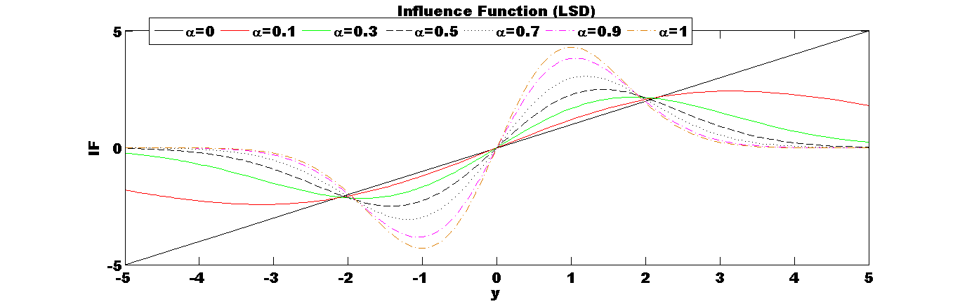
Figure 1: Influence function for the $N(\theta,1)$ Distribution at the model with $\theta=0$

3 Asymptotic Distribution of the Minimum LSD Estimators in Discrete Models

Under the parametric set-up of Section 2.1, consider a discrete family of distributions. We will use the term “density function” generally for the sake of a unified notation, irrespective of whether the distribution is discrete or continuous. Let $X_{1},\ldots,X_{n}$ be a random sample from the true distribution having density function $g$ and let the distribution have support $\chi=\{0,1,2,\cdots\}$. Denote the relative frequency at $x$ from the data by $r_{n}(x)=\frac{1}{n}\sum_{i=1}^{n}I_{x}(X_{i})$. Representing the logarithmic $S$-divergence in terms of the parameter $\beta$ and $\gamma$ (as given in Section 2), let $\hat{\theta}_{\beta,\gamma}$ be the estimator obtained by minimizing ${\rm LSD}_{\beta,\gamma}(\hat{g},f_{\theta})$ over $\theta\in\Theta$, where $\hat{g}$ is a suitable nonparametric density estimate of $g$; in the discrete case the vector of relative frequencies $r_{n}$ based on the sample data is the canonical choice for $\hat{g}$.

In this paper we will primarily describe the statistical applications of the minimum distance procedures that are generated by the logarithmic $S$-divergence. However, for the sake of completeness, we also present the asymptotic distribution of the estimators which has been separately established in Maji, Ghosh and Basu (2014).

When $g$ is replaced by $r_{n}$, the estimating equation (8) may be expressed as

$$\sum_{x}M(\delta_{n}(x))f_{\theta}^{1+\beta}(x)w_{\theta}(x)=0,$$ (14)

where

$$w_{\theta}(x)=[B(\theta)u_{\theta}(x)-A(\theta)],$$

$$M(\delta)=\delta^{A}-1,A(\theta)=\sum_{x}f_{\theta}^{1+\beta}(x)u_{\theta}(x),B(\theta)=\sum_{x}f_{\theta}^{1+\beta}(x),$$

$\delta_{n}(x)=\frac{r_{n}(x)}{f_{\theta}(x)}$ and $\delta_{g}^{g}(x)=\frac{g(x)}{f_{\theta^{g}}(x)}$.

Define,

$$J_{g} = E_{g}\left[w_{\theta^{g}}(X)u_{\theta^{g}}^{T}(X)M^{\prime}(\delta_{g}^{g}(X))f_{\theta^{g}}^{\beta}(X)\right]-\sum_{x}M(\delta_{g}^{g}(x))f_{\theta}^{1+\beta}(x)\nabla w_{\theta^{g}}(x)$$ (15)

$$-(1+\beta)\sum_{x}M(\delta_{g}^{g}(x))f_{\theta}^{1+\beta}(x)w_{\theta^{g}}(x)u_{\theta^{g}}(x)$$

and

$$K_{g} = Var_{g}\left[M^{\prime}(\delta_{g}^{g}(X))f_{\theta^{g}}^{\beta}(X)w_{\theta^{g}}(X)\right].$$ (16)

Note that the matrices $J_{g}$ in (10) and (15) are identical. Then, under standard regularity conditions (See Maji, Ghosh and Basu, 2014), it follows that $\hat{\theta}_{\beta,\gamma}$ is consistent for ${\theta}$ and has the asymptotic distribution given by

$$n^{\frac{1}{2}}(\hat{\theta}_{\beta,\gamma}-\theta)\rightarrow N(0,J_{g}^{-1}K_{g}J_{g}^{-1}),$$ (17)

as $J_{g}$ and $K_{g}$ are as defined in (15) and 16. See Maji, Ghosh and Basu (2014) for the technical details of the proof.

Corollary 1.

When the true distribution $G$ belongs to the model family, i.e., $G=F_{\theta}$ for some $\theta\in\Theta$, then $n^{1/2}(\theta_{n}-\theta)$ has asymptotic distribution as $N_{p}(0,J^{-1}VJ^{-1})$, where

$$J=J_{\beta}(\theta) = E_{g}[w_{\theta}(X)u_{\theta}(X)^{T}f_{\theta}^{\beta}(X)]$$ (18)

$$= \sum_{x}\{B(\theta)u_{\theta}(x)-A(\theta)\}u_{\theta}^{T}(x)f_{\theta}^{1+\beta}(x).$$

$$K=K_{\beta}(\theta) = V_{g}[w_{\theta}(X)f_{\theta}^{\beta}(X)]$$ (19)

$$= \sum_{x}\{B(\theta)u_{\theta}(x)-A(\theta)\}\{B(\theta)u_{\theta}(x)-A(\theta)\}^{T}f_{\theta}^{1+2\beta}(x)$$

$$-\xi\xi^{T},$$

$$\xi=\xi_{\beta}(\theta) = E_{g}[w_{\theta}(X)f_{\theta}^{\beta}(X)]=\sum_{x}\{B(\theta)u_{\theta}(x)-A(\theta)\}f_{\theta}^{1+\beta}(x).$$ (20)

Note that, under model ($g=f_{\theta}$) both $J$ and $K$ depend only on $\beta$. Thus, the asymptotic distribution of the minimum LSD estimators do not depend on the parameter $\gamma$.

4 Testing Parametric Hypothesis using the LSD Measures

4.1 One Sample problem

We consider a parametric family of densities $\mathcal{F}=\{f_{\theta}:\theta\in\Theta\subseteq\mathbb{R}^{p}\}$ as introduced earlier. Suppose we are given a random sample $X_{1},\ldots,X_{n}$ of size $n$ from the population. Based on this sample, we want to test the hypothesis

$$H_{0}:\theta=\theta_{0}~{}~{}~{}\mbox{against}~{}~{}~{}~{}H_{1}:\theta\neq\theta_{0}.$$

When the model is correctly specified and the null hypothesis is correct, $f_{\theta_{0}}$ is the data generating density. We consider the test statistics based on the LSD with parameter $\beta$ and $\gamma$ defined by

$$W_{\beta,\gamma}(\hat{\theta}_{\beta,\gamma},\theta_{0})=2n~{}{\rm LSD}_{\beta,\gamma}(f_{\hat{\theta}_{\beta,\gamma}},f_{\theta_{0}}),$$ (21)

where ${\rm LSD}_{\beta,\gamma}(f_{\hat{\theta}_{\beta,\gamma}},f_{\theta_{0}})$ has the form given in (2). Then the following theorem becomes useful in obtaining the critical values of the test statistics in (21).

Theorem 1.

The asymptotic distribution of the test statistic $W_{\beta,\gamma}(f_{{\hat{\theta}}_{\beta,\gamma}},f_{{\theta_{0}}})$, under the null hypothesis $H_{0}:\theta=\theta_{0}$, coincides with the distribution of

$$\sum_{i=1}^{r}~{}\zeta_{i}^{\beta}(\theta_{0})Z_{i}^{2}$$

where $Z_{1},\ldots,Z_{r}$ are independent standard normal variables, $\zeta_{1}^{\beta}(\theta_{0}),\ldots,\\ \zeta_{r}^{\beta}(\theta_{0})$ are the nonzero eigenvalues of $A_{\beta}(\theta_{0})J_{\beta}^{-1}(\theta_{0})K_{\beta}(\theta_{0})J_{\beta}^{-1}(\theta_{0})$, with $J_{\beta}(\cdot)$ and $K_{\beta}(\cdot)$ as defined in (15) and the matrix $A_{\beta}(\theta_{0})$ is defined as

$$A_{\beta}(\theta_{0})=\nabla[\nabla{\rm LSD}_{\beta,\gamma}(f_{\theta},f_{\theta_{0}})]|_{\theta=\theta_{0}}$$

and

$$r=rank\left(J_{\beta}^{-1}(\theta_{0})K_{\beta}(\theta_{0})J_{\beta}^{-1}(\theta_{0})A_{\beta}(\theta_{0})J_{\beta}^{-1}(\theta_{0})K_{\beta}(\theta_{0})J_{\beta}^{-1}(\theta_{0})\right).$$

Here $\nabla$ represents the gradient with respect to $\theta$.

To see the robustness properties of the LSD based test, we study the influence function analysis of the test statistics as in Hampel et al. (1986), Ghosh and Basu (2014) etc. We define the corresponding LSD based test functional (LSDT) for one sample simple hypothesis problem as described above as (ignoring the sample size dependent multiplier)

$$T_{\beta,\gamma}^{(1)}(G)={\rm LSD}_{\beta,\gamma}\left(f_{T_{\beta,\gamma}(G)},f_{\theta_{0}}\right),$$

where $T_{\beta,\gamma}(G)$ is the minimum LSD functional defined in Section 2.2. Then, considering the contaminated distribution $G_{\epsilon}$ associated with $g_{\epsilon}$, Hampel’s first-order influence function of the LSDT functional turns out to be zero at the null distribution $G=F_{\theta_{0}}$. However, corresponding second order influence function of the LSDT functional at the null distribution has a non-zero form given by

$$IF_{2}(y;T_{\beta,\gamma}^{(1)},F_{\theta_{0}})=IF(y;T_{\beta,\gamma},F_{\theta_{0}})^{T}A_{\beta}(\theta_{0})IF(y;T_{\beta,\gamma},F_{\theta_{0}}).$$ (22)

Therefore the robustness of the LSDT functional depends directly on the robustness of the minimum LSD estimator used in constructing the test statistics. So, following the arguments of Section 2.2 it follows that, the proposed test will have bounded influence function whenever $\beta>0$ implying its robustness and has unbounded influence function at $\beta=0$ implying the lack of robustness. Figure 2 shows the second order influence function of the $N(\theta,1)$ model at the simple null $\theta=0$; the equivalence with the corresponding influence function of the minimum LSD estimator presented in Figure 1 is quite clear.

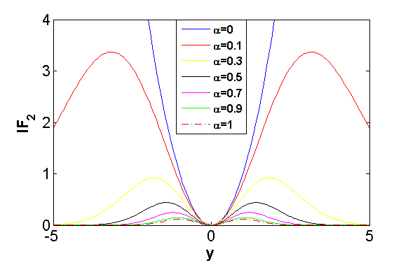
Figure 2: Influence function of the LSD test statistics of normal mean at the null $H_{0}:\theta=0$

4.2 Two Sample Problem

Again consider a parametric family of densities $\{f_{\theta}:\theta\in\Theta\subseteq\mathbb{R}^{p}\}$ as above in one sample problem, but here we are given two random samples $X_{1},\ldots,X_{n}$ of size $n$ and $Y_{1},\ldots,Y_{m}$ of size $m$ from two populations having parameters $\theta_{1}$ and $\theta_{2}$ respectively and based on these two samples, we want to test for the homogeneity of the two samples, i.e. to test the hypothesis

$$H_{0}:\theta_{1}=\theta_{2}~{}~{}~{}\mbox{against}~{}~{}~{}~{}H_{1}:\theta_{1}\neq\theta_{2}.$$

We will consider the estimator ${}^{(1)}\hat{\theta}_{\beta,\gamma}$ and ${}^{(2)}\hat{\theta}_{\beta,\gamma}$ of $\theta_{1}$ and $\theta_{2}$ respectively, obtained by minimizing the LSD having parameter ${\beta,\gamma}$ and then as before, we consider the test statistic based on the LSD with parameter $\beta$ and $\gamma$ as follows

$$S_{\beta,\gamma}\left({}^{(1)}\hat{\theta}_{\beta,\gamma},^{(2)}\hat{\theta}_{\beta,\gamma}\right)=\frac{2nm}{n+m}~{}{\rm LSD}_{\beta,\gamma}\left(f_{{}^{(1)}\hat{\theta}_{\beta,\gamma}},f_{{}^{(2)}\hat{\theta}_{\beta,\gamma}}\right).$$ (23)

We present the asymptotic distribution of the test statistics
$S_{\beta,\gamma}\left({}^{(1)}\hat{\theta}_{\beta,\gamma},^{(2)}\hat{\theta}_{\beta,\gamma}\right)$ under $H_{0}$ in the following theorem.

Theorem 2.

The asymptotic distribution of the test statistic
$S_{\beta,\gamma}\left({}^{(1)}\hat{\theta}_{\beta,\gamma},^{(2)}\hat{\theta}_{\beta,\gamma}\right)$, under the null hypothesis $H_{0}:\theta_{1}=\theta_{2}$, coincides with the distribution of

$$\sum_{i=1}^{r}~{}\zeta_{i}^{\beta}(\theta_{1})Z_{i}^{2}$$

where $Z_{1},\ldots,Z_{r}$ are independent standard normal variables, $\zeta_{1}^{\beta}(\theta_{1}),\ldots,\\ \zeta_{r}^{\beta}(\theta_{1})$ are the nonzero eigenvalues of $A_{\beta}(\theta_{1})J_{\beta}^{-1}(\theta_{1})K_{\beta}(\theta_{1})J_{\beta}^{-1}(\theta_{1})$, with
$J_{\beta}(\cdot)$, $K_{\beta}(\cdot)$ and $A_{\beta}(\cdot)$ as defined in previous section and

$$r=rank\left(J_{\beta}^{-1}(\theta_{1})K_{\beta}(\theta_{1})J_{\beta}^{-1}(\theta_{1})A_{\beta}(\theta_{1})J_{\beta}^{-1}(\theta_{1})K_{\beta}(\theta_{1})J_{\beta}^{-1}(\theta_{1})\right).$$

5 Numerical Illustrations

5.1 Performance of the Minimum LSD Estimator : Simulation in the Poisson Model

To explore the performance of the proposed minimum LSD estimators, we have done several simulation studies under the Poisson model with sample size of $n=50$. We simulate data from a Poisson distribution with parameter $\theta=4$ and compute the empirical bias and the MSE of the minimum LSD estimators of $\theta$ based on 1000 replications. The results obtained are reported in Tables 1 and 2 respectively. Clearly both the bias and MSE are quite small for any $(\beta,\gamma)$ combination; however the MSE increases slightly with $\beta$.

Table 1: The Empirical bias of the minimum LSD estimators for different values of $\beta$ and $\gamma$

$\gamma$	$\beta=0$	$\beta=0.1$	$\beta=0.2$	$\beta=0.4$	$\beta=0.5$	$\beta=0.6$	$\beta=0.8$	$\beta=1$
$-1$	$-1.104$	$-0.336$	$-0.186$	$-0.055$	$-0.035$	$-0.013$	0.006	0.015
$-0.9$	$-0.360$	$-0.202$	$-0.124$	$-0.050$	$-0.028$	$-0.012$	$-0.003$	0.010
$-0.7$	$-0.169$	$-0.113$	$-0.073$	$-0.029$	$-0.019$	$-0.008$	0.002	0.006
$-0.5$	$-0.095$	$-0.065$	$-0.044$	$-0.016$	$-0.004$	$-0.004$	0.008	0.016
$-0.3$	$-0.049$	$-0.030$	$-0.020$	$-0.003$	$-0.001$	$-0.002$	0.004	0.020
$-0.1$	$-0.015$	$-0.010$	$-0.002$	0.006	0.011	0.012	0.014	0.015
0	0.000	0.000	0.009	0.017	0.012	0.004	0.007	0.024
0.1	0.014	0.013	0.017	0.018	0.004	0.012	0.014	0.007
0.3	0.038	0.037	0.031	0.023	0.021	0.019	0.014	0.007
0.5	0.060	0.053	0.046	0.030	0.021	0.026	0.019	0.006
0.7	0.080	0.069	0.060	0.039	0.042	0.024	0.020	0.012
0.9	0.098	0.085	0.071	0.048	0.038	0.025	0.019	0.009
1	0.106	0.090	0.077	0.047	0.031	0.031	0.013	0.017
1.5	0.140	0.125	0.108	0.069	0.056	0.023	0.023	0.008
2	0.166	0.150	0.130	0.087	0.067	0.050	0.025	0.006

Table 2: The Empirical MSE of the minimum LSD estimators for different values of $\beta$ and $\gamma$

$\gamma$	$\beta=0$	$\beta=0.1$	$\beta=0.2$	$\beta=0.4$	$\beta=0.5$	$\beta=0.6$	$\beta=0.8$	$\beta=1$
$-1$	6.989	0.415	0.251	0.136	0.147	0.131	0.142	0.148
$-0.9$	0.316	0.179	0.144	0.131	0.124	0.131	0.142	0.154
$-0.7$	0.137	0.124	0.116	0.120	0.129	0.129	0.141	0.140
$-0.5$	0.101	0.101	0.104	0.115	0.122	0.122	0.140	0.153
$-0.3$	0.088	0.091	0.094	0.107	0.117	0.120	0.138	0.152
$-0.1$	0.083	0.090	0.097	0.107	0.114	0.119	0.143	0.154
0	0.083	0.085	0.096	0.108	0.110	0.122	0.136	0.155
0.1	0.082	0.088	0.092	0.106	0.115	0.120	0.134	0.150
0.3	0.084	0.086	0.094	0.106	0.115	0.122	0.133	0.148
0.5	0.087	0.088	0.092	0.102	0.112	0.120	0.139	0.151
0.7	0.092	0.091	0.093	0.102	0.112	0.117	0.128	0.147
0.9	0.099	0.096	0.095	0.103	0.111	0.112	0.129	0.150
1	0.102	0.096	0.093	0.100	0.105	0.117	0.130	0.153
1.5	0.121	0.111	0.104	0.103	0.105	0.109	0.128	0.153
2	0.139	0.127	0.114	0.102	0.103	0.113	0.121	0.152

Next to study the robustness properties of the minimum LSD estimators we repeat the above study, but introduce a contamination in the simulated samples by replacing $10\%$ of it by $Poisson(\theta={\rm 12})$ observations. The corresponding values of the empirical bias and MSE, against the target value of $\theta=3$, are presented in Tables 3 and 4 respectively. Note that, the minimum LSD estimators are seen to be robust for all $\beta\in[0,1]$ if $\gamma<0$ and for suitably large values of $\beta$ if $\gamma\geq 0$. However, the estimators corresponding to small $\beta$ close to zero and $\gamma\geq 0$.

Table 3: The Empirical bias of the minimum LSD estimators under $10\%$ contamination for different values of $\beta$ and $\gamma$

$\gamma$	$\beta=0$	$\beta=0.1$	$\beta=0.2$	$\beta=0.4$	$\beta=0.5$	$\beta=0.6$	$\beta=0.8$	$\beta=1$
$-1$	$-1.407$	$-0.140$	$-0.024$	0.064	0.071	0.087	0.086	0.083
$-0.9$	$-0.134$	$-0.021$	0.027	0.077	0.081	0.081	0.084	0.079
$-0.7$	0.056	0.084	0.090	0.106	0.099	0.089	0.092	0.072
$-0.5$	0.172	0.154	0.141	0.118	0.105	0.103	0.096	0.088
$-0.3$	0.314	0.244	0.202	0.151	0.123	0.104	0.094	0.083
$-0.1$	0.578	0.394	0.283	0.174	0.143	0.123	0.102	0.082
0	0.800	0.519	0.347	0.192	0.160	0.136	0.091	0.082
0.1	1.071	0.697	0.439	0.213	0.160	0.144	0.108	0.085
0.3	1.590	1.165	0.726	0.267	0.188	0.149	0.111	0.084
0.5	1.965	1.604	1.147	0.368	0.237	0.161	0.106	0.077
0.7	2.219	1.929	1.532	0.546	0.289	0.183	0.117	0.081
0.9	2.394	2.161	1.834	0.805	0.390	0.217	0.112	0.079
1	2.461	2.252	1.950	0.958	0.452	0.240	0.115	0.083
1.5	2.671	2.545	2.354	1.627	0.996	0.402	0.132	0.089
2	2.773	2.691	2.568	2.055	1.545	0.792	0.149	0.084

Table 4: The Empirical MSE of the minimum LSD estimators under $10\%$ contamination for different values of $\beta$ and $\gamma$

$\gamma$	$\beta=0$	$\beta=0.1$	$\beta=0.2$	$\beta=0.4$	$\beta=0.5$	$\beta=0.6$	$\beta=0.8$	$\beta=1$
$-1$	7.336	0.419	0.257	0.178	0.183	0.168	0.172	0.183
$-0.9$	0.303	0.207	0.196	0.166	0.187	0.165	0.178	0.183
$-0.7$	0.160	0.159	0.158	0.157	0.166	0.169	0.196	0.176
$-0.5$	0.161	0.162	0.159	0.161	0.165	0.164	0.179	0.184
$-0.3$	0.216	0.184	0.174	0.162	0.158	0.161	0.171	0.185
$-0.1$	0.430	0.268	0.203	0.168	0.158	0.166	0.169	0.177
0	0.732	0.369	0.238	0.167	0.169	0.168	0.167	0.182
0.1	1.276	0.581	0.302	0.184	0.161	0.165	0.172	0.183
0.3	2.836	1.525	0.626	0.200	0.172	0.168	0.175	0.181
0.5	4.343	2.909	1.492	0.251	0.198	0.169	0.170	0.184
0.7	5.524	4.207	2.669	0.409	0.208	0.176	0.166	0.186
0.9	6.401	5.261	3.831	0.772	0.271	0.187	0.166	0.188
1	6.749	5.703	4.328	1.075	0.319	0.194	0.174	0.181
1.5	7.887	7.204	6.222	3.060	1.175	0.284	0.172	0.184
2	8.462	8.001	7.335	4.820	2.779	0.773	0.170	0.188

6 Limitation of the First Order Influence Function & some Remedies

The numeral examples and simulation results presented in the previous section clearly shows that the robustness of minimum LSD estimators in terms of its bias and MSE under data contamination depends on the parameter $\gamma$ for smaller values of $\beta$. However, according to the classical literature, its first order influence function suggests that (see Section 2.2) its robustness will be independent of the parameter $\gamma$ for all values of $\beta$. Thus, the classical approach of robustness measure through the first order influence fails in the case of minimum divergence estimation with the logarithmic super divergence family. Similar limitations of the first order influence functions was also observed by Lindsay (1994) and Ghosh et al. (2013) for the case of power divergence family and the $S$-divergence family; accordingly they have proposed some alternative measure of robustness. In this section, we use some of those alternative measures to explain the robustness of the proposed minimum LSD estimators.

6.1 Higher Order Influence Analysis

The higher (second) order influence function analysis for studying the robustness of a minimum divergence estimators was used by Lindsay (1994) for the case of PD family and recently by Ghosh et al. (2013) for the $S$-divergence family; both the work have shown this approach to provide significantly improved prediction of the robustness of corresponding estimators. Here, we present a similar analysis for the minimum LSD estimator.

For any functional $T$, $\Delta T(\epsilon)=T(G_{\epsilon})-T(G)$ quantifies the amount of bias under contamination as a function of contamination proportion $\epsilon$, which can be approximated using the first-order Taylor expansion as $\Delta T(\epsilon)=T(G_{\epsilon})-T(G)\approx\epsilon T^{\prime}(y)$. Hence the first order influence function gives an approximation to the predicted bias up to first order. When this first order approximation fails, we can consider a second order (approximate) bias prediction by $\Delta T(\epsilon)=\epsilon T^{\prime}(y)+\frac{\epsilon^{2}}{2}T^{\prime\prime}(y)$. The term $T^{\prime\prime}(y)$ is interpreted as the second order influence function and the ratio

$$\frac{\mbox{quadratic approximation}}{\mbox{linear approximation}}=1+\frac{[T^{\prime\prime}(y)/T^{\prime}(y)]\epsilon}{2}$$

serve as a measure of adequacy of the first-order approximation and hence of the first order influence analysis; the two approximation may differ significantly for fairly small values of $\epsilon$ when the first order approximation is inadequate. Our next theorem present the expression of the second order approximation $T^{\prime\prime}(y)$ for the minimum LSD estimator with a scalar parameter; this can be routinely extended to the case of vector parameter also. Let us define, for the model family $\{f_{\theta}\}$ with a scalar $\theta$, the quantities $c_{i}=\int u_{\theta}^{i}f_{\theta}^{1+\beta}$ and $d_{i}=\int[\nabla u_{\theta}]u_{\theta}^{i}f_{\theta}^{1+\beta}$ for $i=0,1,2,3$.

Theorem 1.

Under the above mentioned set-up with a scalar parameter $\theta$, if true distribution belonging to the model family then the second order influence function of the minimum LSD estimator defined by the estimating equation (8) is

$$T^{\prime\prime}(y)=(N_{0}^{p}D_{0}-N_{0}D_{0}^{p})/D_{0}^{2}.$$

where

$$N_{0} = f_{\theta}^{\beta}(y)u_{\theta}(y)c_{o}-f_{\theta}^{\beta}(y)c_{1},$$

$$D_{0} = c_{2}c_{0}-c_{1}^{2},$$

$$N_{0}^{p} = BT^{\prime}(y)c_{1}^{2}-(A-1)c_{1}c_{0}+2(A-1)f_{\theta}^{\beta}(y)c_{1}$$

$$-BT^{\prime}(y)f_{\theta}^{\beta}(y)u_{\theta}(y)c_{1}-(A-1)f_{\theta}^{\beta-1}(y)c_{1}$$

$$-BT^{\prime}(y)c_{2}c_{0}-T^{\prime}(y)d_{0}c_{0}+BT^{\prime}(y)f_{\theta}^{\beta}(y)u_{\theta}^{2}(y)c_{0}$$

$$+f_{\theta}^{\beta}(y)u_{\theta}^{\prime}(y)T^{\prime}(y)c_{0}-(A-1)f_{\theta}^{\beta}(y)u_{\theta}(y)c_{0}$$

$$+(A-1)f_{\theta}^{\beta-1}(y)u_{\theta}(y)c_{0}-(1+\beta)f_{\theta}^{\beta}(y)u_{\theta}(y)T^{\prime}(y)c_{1}$$

$$+(1+\beta)T^{\prime}(y)c_{0}c_{2}-(1+\beta)T^{\prime}(y)f_{\theta}^{\beta}(y)c_{2}$$

$${\rm and}$$

$$D_{0}^{p} = (A^{2}+2AB)T^{\prime}(y)c_{3}c_{0}+3AT^{\prime}(y)d_{1}c_{0}+B(1+\beta)T^{\prime}(y)c_{2}c_{0}-A^{2}c_{2}c_{0}$$

$$+A(1+\beta)f_{\theta}^{\beta}(y)c_{2}-(A+\beta)T^{\prime}(y)d_{0}c_{1}+Af_{\theta}^{\beta}(y)d_{0}$$

$$-(AB+A(1+\beta)+(1+\beta)B)T^{\prime}(y)c_{2}c_{1}+A^{2}c_{1}^{2}-A^{2}f_{\theta}^{\beta}(y)u_{\theta}(y)c_{1}$$

$$-ABf_{\theta}^{\beta}(y)u_{\theta}^{2}(y)c_{0}-Af_{\theta}^{\beta}(y)u_{\theta}^{\prime}(y)c_{0},$$

where $u_{\theta}^{\prime}(y)=\frac{\partial}{\partial\theta}u_{\theta}(y).$

Example (Poisson Mean): Let us now consider a numerical simulation to study the performance of the above second order influence analysis through its application in case of the Poisson model with mean $\theta$. Using the special structure of one parameter exponential family, of which Poisson distribution is a special case, we compute the first and second order bias approximation using their respective expressions as given above and in Section 2.2. However, for brevity, we will only present some particular simulation result with $\theta=4$, the contamination point $y=12$ and specific $(\beta,\gamma)$ combinations and the corresponding bias plots are shown in Figures 3, 4 and 5 respectively for $\gamma=0$, $\gamma>0$ and $\gamma<0$.

Comments on Figure 3 $(\gamma=0)$: As expected both first order and second order influence function for $\beta=0$ gives a straight line. The bias approximation decreases as $\beta$ increases for both first and second order influence function. The difference of approximation between first and second order decreases as $\beta$ increases.

Comments on Figure 4 $(\gamma>0)$: Keeping $\gamma$ fixed the difference between bias approximation among first and second order decreases as $\beta$ increases.

Comments on Figure 5 $(\gamma<0)$: As expected for this case the bias approximation is more for the first order influence function compared to the second order but the difference among two types of influence function shows same behavior compared to the case $\gamma>0$.

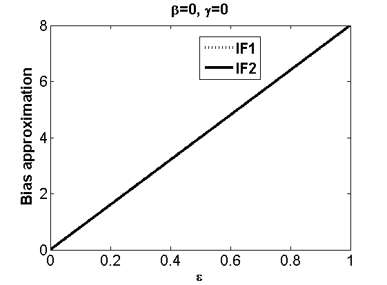
(a) $\beta=0$, $\gamma=0$

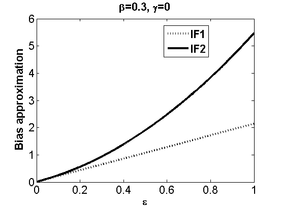
(b) $\beta=0.3$, $\gamma=0$

(c) $\beta=0.6$, $\gamma=0$

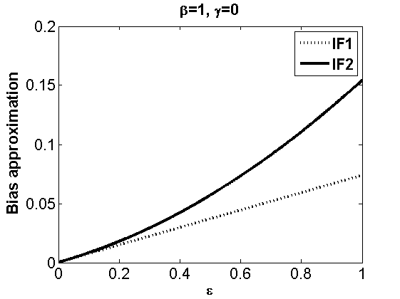
(d) $\beta=1$, $\gamma=0$

Figure 3: Bias Approximations (solid line : second order; dashed line : first order) for the minimum LSD estimator for $\gamma=0$

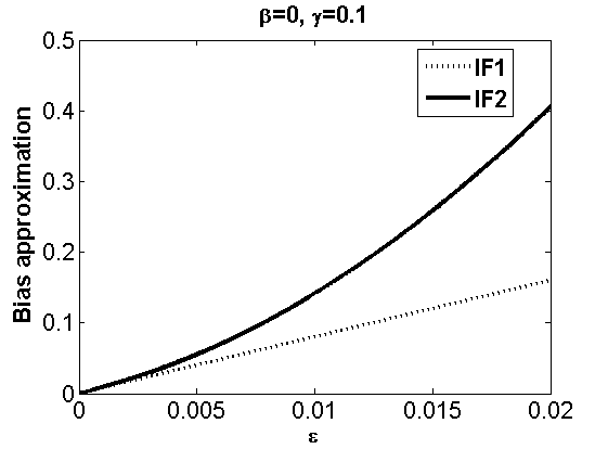
(a) $\beta=0$, $\gamma=0.1$

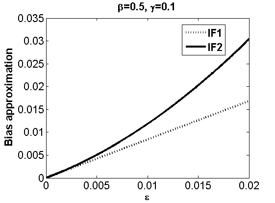
(b) $\beta=0.5$, $\gamma=0.1$

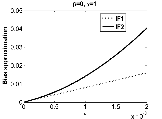
(c) $\beta=0$, $\gamma=1$

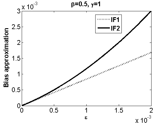
(d) $\beta=0.5$, $\gamma=1$

Figure 4: Bias Approximations (solid line : second order; dashed line : first order) for the minimum LSD estimator for $\gamma>0$

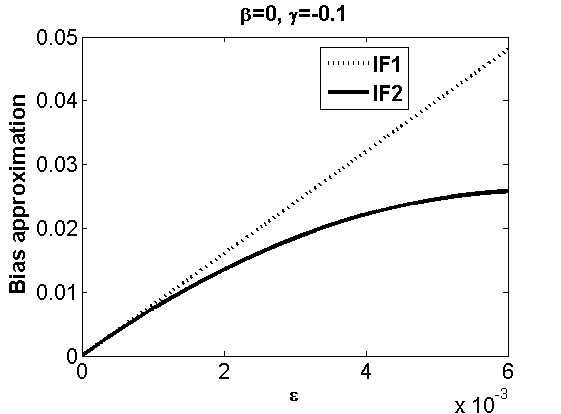
(a) $\beta=0$, $\gamma=-0.1$

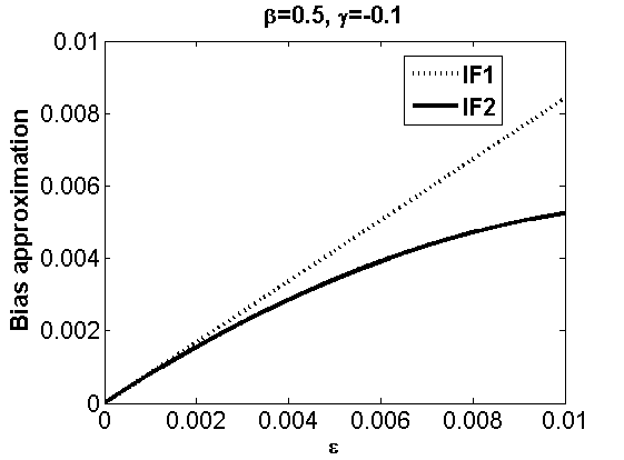
(b) $\beta=0.5$, $\gamma=-0.1$

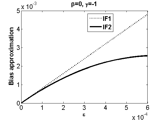
(c) $\beta=0$, $\gamma=-1$

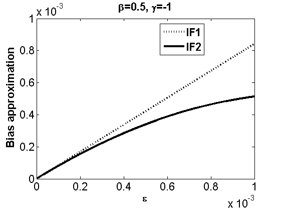
(d) $\beta=0.5$, $\gamma=-1$

Figure 5: Bias Approximations (solid line : second order; dashed line : first order) for the minimum LSD estimator for $\gamma<0$

6.2 A Breakdown Point Result : Location Model

Another popular alternative to the influence function analysis is the breakdown point theory; following Simpson (1987) we will say that the estimator $T(G)$ breaks down for contamination level $\epsilon$ if $|T_{\beta,\gamma}(H_{\epsilon,n})-T(G)|œ\rightarrow\infty$ as $n\rightarrow\infty$ for some sequence $K_{n}$ and $H_{\epsilon,n}=(1-\epsilon)G+\epsilon K_{n}$. Although the derivation of a general breakdown result is difficult, several authors have used it for some suitable subclass of probability distributions; see Park and Basu (2004), Ghosh et al. (2013) for breakdown results on some related minimum divergence estimators.

Now we derive the breakdown point of the minimum LSD functional
$T_{\beta,\gamma}(G)$ under the special class of location family $\mathcal{F}_{\theta}=\{f_{\theta}(x)=f(x-\theta):\theta\in\Theta\}$. The particular property of this family, that helps to make the calculations simpler, is

$$\int\{f(x-\theta)\}^{1+\beta}dx=\int\{f(x)\}^{1+\beta}dx=M_{f}^{\beta},~{}~{}~{}~{}\mbox{(say)}$$

which is independent of the parameter $\theta$. Using this and the increasing nature of the logarithmic function, the minimum LSD estimator for a location model is seen to be the maximizer of only the one integral term $\int f^{B}g^{A}$ whenever $A>0$ and $B>0$. However, under the same location model the minimum $S$-divergence estimator of Ghosh et al. (2013) can also be seen to be the maximizer of the same integral. Therefore, under the location family of densities, the minimum LSD estimator with $A>0$ and $B>0$ coincides with corresponding minimum $S$-divergence estimators. Then it follows from Ghosh et al. (2013) that, under certain assumptions (assumptions BP1 to BP3 of their paper) the asymptotic breakdown point $\epsilon^{*}$ of the minimum LSD estimator $T_{\beta,\gamma}$ with $A>0$ and $B>0$ is at least $\frac{1}{2}$ at the model family.

7 Testing Hypotheses Simulation

This section will describe the testing of hypotheses simulation example. We have taken sample from $(1-\epsilon)\mbox{ Poisson}(2)+\epsilon\mbox{ Poisson}(15)$ for $\epsilon=0,0.1$ and various sample sizes $n=20,50,100$. All simulations have been replicated $1000$ times. Tables 5, 6 and 7 give us the observed levels for no contamination case and tables 11, 12 and 13 for contamination case while testing $H_{0}:\theta=2$ and the powers given in tables 8, 9 and 10 for no contamination case and 14, 15 and 16 for contamination case considering the testing problem $H_{0}:\theta=3$. Here the observed level has been taken as $0.05$. Usually for both $\beta$ and $\gamma$ close to $0$ we get level close to $0.05$ under no contamination case. For $\beta\geq 0.04$, level does not go under $0.06$ for any $\gamma$. As $\gamma$ becomes distant from $0$ in both positive and negative direction level moves from $0.05$ under no contamination. Under contamination set-up, empirical level usually does not go below than $0.1$. For smaller sample size like $20$ level never become lower than $0.1$ whereas for large sample size as $100$, only when $-0.5\leq\gamma\leq-0.3$ and $\beta\leq 0.2$ level becomes lower than $0.1$ and for moderately large sample size $50$, the situation does not differ very significantly. Under contamination set-up for $\beta\leq 0.4$ and $\gamma>0$, the level is very high and for sample size $100$ it goes to $1$ also. The empirical power is very high under no contamination. For sample size $100$ the power is $1$ for most of the values of $\beta$ and $\gamma$. Though for sample size $50$ the power does not reach $1$ but it is usually very close to $1$. Power usually does not go to that close to $1$ for sample size $20$ except for high negative value of $\gamma(\leq-0.5)$ and lower value of $\beta(\leq 0.2)$. Under contamination set-up and for sample size $20$ the power usually does not go to $1$ but for low $\beta$ and high negative value of $\gamma$ it goes very close. For $\gamma$ close to $0$ and low $\beta$, the power becomes less than $0.5$ but this is not much common throughout the table. For sample size $100$, the power is usually becomes $1$ except for very few combinations of $(\beta,\gamma)$ and this fact is maintained for sample size $50$ also. As shown earlier, for $\beta=1$, the divergence is independent of $\gamma$, that fact is also evident from the result that both level and power for all values of $\gamma$ is same for $\beta=1$.

Table 5: The Empirical level of the LSD statistic under $H_{0}:\theta=2$ for different values of $\beta$ and $\gamma$ ($n=20$) (No Contamination)

$\gamma$	$\beta=0$	$\beta=0.1$	$\beta=0.2$	$\beta=0.4$	$\beta=0.7$	$\beta=0.8$	$\beta=0.9$	$\beta=1$
$-1$	–	0.629	0.35	0.171	0.119	0.123	0.131	0.135
$-0.9$	0.673	0.418	0.264	0.143	0.118	0.123	0.13	0.135
$-0.7$	0.294	0.209	0.165	0.126	0.115	0.123	0.131	0.135
$-0.5$	0.149	0.133	0.118	0.111	0.113	0.123	0.13	0.135
$-0.3$	0.104	0.098	0.101	0.103	0.111	0.121	0.128	0.135
$-0.1$	0.078	0.084	0.083	0.097	0.109	0.12	0.127	0.135
0	0.041	0.08	0.081	0.093	0.11	0.118	0.127	0.135
0.1	0.073	0.078	0.079	0.092	0.112	0.118	0.126	0.135
0.3	0.074	0.072	0.074	0.085	0.113	0.115	0.126	0.135
0.5	0.081	0.076	0.075	0.087	0.109	0.117	0.127	0.135
0.7	0.101	0.085	0.078	0.083	0.109	0.117	0.128	0.135
0.9	0.118	0.1	0.084	0.083	0.108	0.119	0.128	0.135
1	0.128	0.111	0.089	0.083	0.109	0.119	0.127	0.135
1.5	0.159	0.154	0.13	0.089	0.105	0.114	0.127	0.135
2	0.16	0.164	0.163	0.112	0.103	0.112	0.122	0.135

Table 6: The Empirical level of the LSD statistic under $H_{0}:\theta=2$ for different values of $\beta$ and $\gamma$ ($n=50$) (No Contamination)

$\gamma$	$\beta=0$	$\beta=0.1$	$\beta=0.2$	$\beta=0.4$	$\beta=0.7$	$\beta=0.8$	$\beta=0.9$	$\beta=1$
$-1$	–	0.439	0.204	0.093	0.079	0.091	0.099	0.102
$-0.9$	0.56	0.241	0.142	0.086	0.078	0.089	0.097	0.102
$-0.7$	0.187	0.118	0.089	0.074	0.077	0.087	0.097	0.102
$-0.5$	0.09	0.078	0.07	0.064	0.077	0.087	0.097	0.102
$-0.3$	0.066	0.063	0.063	0.061	0.078	0.085	0.097	0.102
$-0.1$	0.053	0.054	0.059	0.063	0.077	0.084	0.096	0.102
0	0.05	0.053	0.057	0.061	0.076	0.084	0.096	0.102
0.1	0.047	0.054	0.055	0.06	0.075	0.085	0.096	0.102
0.3	0.054	0.053	0.058	0.061	0.076	0.084	0.095	0.102
0.5	0.068	0.059	0.057	0.062	0.074	0.084	0.094	0.102
0.7	0.093	0.073	0.061	0.061	0.073	0.084	0.094	0.102
0.9	0.12	0.09	0.07	0.06	0.073	0.083	0.093	0.102
1	0.123	0.102	0.075	0.061	0.074	0.083	0.093	0.102
1.5	0.157	0.139	0.117	0.068	0.073	0.084	0.091	0.102
2	0.218	0.165	0.145	0.084	0.073	0.08	0.092	0.102

Table 7: The Empirical level of the LSD statistic under $H_{0}:\theta=2$ for different values of $\beta$ and $\gamma$ ($n=100$) (No Contamination)

$\gamma$	$\beta=0$	$\beta=0.1$	$\beta=0.2$	$\beta=0.4$	$\beta=0.7$	$\beta=0.8$	$\beta=0.9$	$\beta=1$
$-1$	–	0.373	0.141	0.087	0.102	0.111	0.117	0.127
$-0.9$	0.444	0.176	0.114	0.08	0.102	0.111	0.117	0.127
$-0.7$	0.131	0.098	0.083	0.078	0.1	0.11	0.118	0.127
$-0.5$	0.078	0.071	0.076	0.075	0.099	0.108	0.119	0.127
$-0.3$	0.061	0.061	0.066	0.079	0.099	0.108	0.119	0.127
$-0.1$	0.054	0.057	0.063	0.076	0.099	0.109	0.12	0.127
0	0.048	0.057	0.06	0.075	0.1	0.109	0.12	0.127
0.1	0.054	0.055	0.06	0.076	0.1	0.109	0.12	0.127
0.3	0.062	0.06	0.061	0.077	0.099	0.109	0.12	0.127
0.5	0.075	0.065	0.058	0.077	0.1	0.109	0.118	0.127
0.7	0.082	0.075	0.062	0.078	0.099	0.109	0.119	0.127
0.9	0.112	0.08	0.072	0.077	0.098	0.11	0.118	0.127
1	0.122	0.09	0.077	0.078	0.098	0.11	0.118	0.127
1.5	0.196	0.146	0.108	0.08	0.095	0.109	0.116	0.127
2	0.231	0.208	0.155	0.095	0.096	0.107	0.116	0.127

Table 8: The Empirical power of the LSD statistic under $H_{0}:\theta=3$ against $H_{1}:\theta=2$ for different values of $\beta$ and $\gamma$ ($n=20$)(No Contamination)

$\gamma$	$\beta=0$	$\beta=0.1$	$\beta=0.2$	$\beta=0.4$	$\beta=0.7$	$\beta=0.8$	$\beta=0.9$	$\beta=1$
$-1$	–	0.997	0.98	0.948	0.885	0.865	0.853	0.834
$-0.9$	0.998	0.991	0.969	0.939	0.88	0.864	0.851	0.834
$-0.7$	0.973	0.965	0.956	0.917	0.874	0.861	0.85	0.834
$-0.5$	0.955	0.938	0.922	0.895	0.865	0.856	0.848	0.834
$-0.3$	0.912	0.899	0.889	0.876	0.858	0.851	0.847	0.834
$-0.1$	0.868	0.865	0.863	0.86	0.854	0.85	0.846	0.834
0	0.828	0.85	0.853	0.855	0.853	0.85	0.846	0.834
0.1	0.838	0.838	0.846	0.847	0.851	0.849	0.846	0.834
0.3	0.808	0.816	0.826	0.84	0.847	0.85	0.843	0.834
0.5	0.766	0.791	0.805	0.827	0.841	0.842	0.842	0.834
0.7	0.739	0.759	0.778	0.808	0.829	0.836	0.84	0.834
0.9	0.721	0.736	0.753	0.797	0.827	0.833	0.838	0.834
1	0.704	0.725	0.746	0.791	0.826	0.831	0.837	0.834
1.5	0.647	0.677	0.701	0.754	0.813	0.824	0.831	0.834
2	0.609	0.637	0.67	0.726	0.795	0.814	0.825	0.834

Table 9: The Empirical power of the LSD statistic under $H_{0}:\theta=3$ against $H_{1}:\theta=2$ for different values of $\beta$ and $\gamma$ ($n=50$)(No Contamination)

$\gamma$	$\beta=0$	$\beta=0.1$	$\beta=0.2$	$\beta=0.4$	$\beta=0.7$	$\beta=0.8$	$\beta=0.9$	$\beta=1$
$-1$	–	0.999	0.999	0.997	0.994	0.991	0.99	0.987
$-0.9$	0.999	0.999	0.998	0.996	0.994	0.991	0.99	0.987
$-0.7$	0.999	0.998	0.998	0.995	0.994	0.991	0.99	0.987
$-0.5$	0.997	0.996	0.997	0.995	0.992	0.991	0.99	0.987
$-0.3$	0.996	0.996	0.995	0.994	0.991	0.991	0.99	0.987
$-0.1$	0.996	0.994	0.994	0.993	0.991	0.99	0.989	0.987
0	0.994	0.995	0.993	0.993	0.991	0.99	0.989	0.987
0.1	0.995	0.994	0.992	0.993	0.991	0.99	0.989	0.987
0.3	0.992	0.994	0.993	0.993	0.991	0.99	0.989	0.987
0.5	0.99	0.991	0.993	0.992	0.99	0.989	0.989	0.987
0.7	0.986	0.989	0.99	0.991	0.989	0.989	0.989	0.987
0.9	0.977	0.988	0.987	0.99	0.989	0.989	0.989	0.987
1	0.975	0.986	0.987	0.989	0.989	0.989	0.989	0.987
1.5	0.963	0.971	0.981	0.988	0.989	0.988	0.988	0.987
2	0.951	0.96	0.967	0.985	0.988	0.988	0.988	0.987

Table 10: The Empirical power of the LSD statistic under $H_{0}:\theta=3$ against $H_{1}:\theta=2$ for different values of $\beta$ and $\gamma$ ($n=100$)(No Contamination)

$\gamma$	$\beta=0$	$\beta=0.1$	$\beta=0.2$	$\beta=0.4$	$\beta=0.7$	$\beta=0.8$	$\beta=0.9$	$\beta=1$
$-1$	–	1	1	1	1	1	1	1
$-0.9$	1	1	1	1	1	1	1	1
$-0.7$	1	1	1	1	1	1	1	1
$-0.5$	1	1	1	1	1	1	1	1
$-0.3$	1	1	1	1	1	1	1	1
$-0.1$	1	1	1	1	1	1	1	1
0	1	1	1	1	1	1	1	1
0.1	1	1	1	1	1	1	1	1
0.3	1	1	1	1	1	1	1	1
0.5	1	1	1	1	1	1	1	1
0.7	0.999	1	1	1	1	1	1	1
0.9	0.998	0.999	1	1	1	1	1	1
1	0.995	0.999	1	1	1	1	1	1
1.5	0.993	0.994	0.999	1	1	1	1	1
2	0.987	0.993	0.994	1	1	1	1	1

Table 11: The Empirical level of the LSD statistic under $H_{0}:\theta=2$ for different values of $\beta$ and $\gamma$ ($n=20$) ($90\%{\rm Poisson}(2)+10\%{\rm Poisson}(15)$)

$\gamma$	$\beta=0$	$\beta=0.1$	$\beta=0.2$	$\beta=0.4$	$\beta=0.7$	$\beta=0.8$	$\beta=0.9$	$\beta=1$
$-1$	–	0.647	0.388	0.205	0.162	0.164	0.171	0.173
$-0.9$	0.685	0.435	0.289	0.177	0.16	0.164	0.171	0.173
$-0.7$	0.316	0.242	0.194	0.156	0.153	0.16	0.168	0.173
$-0.5$	0.175	0.161	0.15	0.142	0.151	0.159	0.167	0.173
$-0.3$	0.122	0.126	0.126	0.133	0.15	0.157	0.164	0.173
$-0.1$	0.233	0.112	0.113	0.13	0.145	0.156	0.163	0.173
0	0.684	0.216	0.119	0.126	0.144	0.152	0.162	0.173
0.1	0.863	0.637	0.15	0.127	0.141	0.152	0.161	0.173
0.3	0.883	0.87	0.778	0.123	0.14	0.152	0.159	0.173
0.5	0.885	0.881	0.87	0.178	0.14	0.148	0.157	0.173
0.7	0.889	0.884	0.88	0.653	0.14	0.146	0.157	0.173
0.9	0.892	0.887	0.883	0.849	0.141	0.145	0.156	0.173
1	0.894	0.891	0.885	0.865	0.141	0.145	0.156	0.173
1.5	0.897	0.896	0.892	0.882	0.138	0.146	0.154	0.173
2	0.897	0.898	0.897	0.888	0.17	0.147	0.155	0.173

Table 12: The Empirical level of the LSD statistic under $H_{0}:\theta=2$ for different values of $\beta$ and $\gamma$ ($n=50$) ($90\%{\rm Poisson}(2)+10\%{\rm Poisson}(15)$)

$\gamma$	$\beta=0$	$\beta=0.1$	$\beta=0.2$	$\beta=0.4$	$\beta=0.7$	$\beta=0.8$	$\beta=0.9$	$\beta=1$
$-1$	–	0.436	0.214	0.111	0.105	0.114	0.128	0.14
$-0.9$	0.545	0.256	0.16	0.102	0.104	0.114	0.128	0.14
$-0.7$	0.191	0.125	0.106	0.085	0.103	0.113	0.128	0.14
$-0.5$	0.099	0.094	0.088	0.083	0.102	0.112	0.128	0.14
$-0.3$	0.087	0.078	0.078	0.082	0.103	0.111	0.126	0.14
$-0.1$	0.402	0.123	0.08	0.081	0.102	0.109	0.126	0.14
0	0.937	0.333	0.102	0.083	0.101	0.11	0.125	0.14
0.1	0.986	0.867	0.222	0.085	0.101	0.109	0.125	0.14
0.3	0.995	0.987	0.951	0.093	0.103	0.108	0.125	0.14
0.5	0.996	0.995	0.988	0.213	0.101	0.108	0.124	0.14
0.7	0.996	0.996	0.994	0.824	0.099	0.106	0.122	0.14
0.9	0.996	0.996	0.996	0.979	0.1	0.106	0.122	0.14
1	0.996	0.996	0.996	0.986	0.1	0.106	0.12	0.14
1.5	0.998	0.998	0.997	0.996	0.103	0.105	0.12	0.14
2	0.998	0.998	0.998	0.997	0.139	0.104	0.119	0.14

Table 13: The Empirical level of the LSD statistic under $H_{0}:\theta=2$ for different values of $\beta$ and $\gamma$ ($n=100$) ($90\%{\rm Poisson}(2)+10\%{\rm Poisson}(15)$)

$\gamma$	$\beta=0$	$\beta=0.1$	$\beta=0.2$	$\beta=0.4$	$\beta=0.7$	$\beta=0.8$	$\beta=0.9$	$\beta=1$
$-1$	–	0.371	0.174	0.107	0.118	0.128	0.138	0.141
$-0.9$	0.434	0.202	0.131	0.111	0.117	0.128	0.137	0.141
$-0.7$	0.152	0.108	0.094	0.112	0.116	0.129	0.136	0.141
$-0.5$	0.09	0.086	0.092	0.106	0.117	0.129	0.136	0.141
$-0.3$	0.095	0.091	0.087	0.101	0.118	0.128	0.136	0.141
$-0.1$	0.625	0.167	0.103	0.101	0.117	0.128	0.136	0.141
0	0.996	0.488	0.131	0.099	0.117	0.126	0.136	0.141
0.1	1	0.969	0.293	0.103	0.116	0.125	0.136	0.141
0.3	1	1	0.997	0.112	0.116	0.125	0.135	0.141
0.5	1	1	1	0.236	0.115	0.126	0.134	0.141
0.7	1	1	1	0.914	0.115	0.125	0.135	0.141
0.9	1	1	1	0.999	0.115	0.124	0.135	0.141
1	1	1	1	0.999	0.116	0.124	0.135	0.141
1.5	1	1	1	1	0.118	0.124	0.134	0.141
2	1	1	1	1	0.164	0.123	0.133	0.141

Table 14: The Empirical power of the LSD statistic under $H_{0}:\theta=3$ against $H_{1}:\theta=2$ for different values of $\beta$ and $\gamma$ ($n=20$) ($90\%{\rm Poisson}(2)+10\%{\rm Poisson}(15)$)

$\gamma$	$\beta=0$	$\beta=0.1$	$\beta=0.2$	$\beta=0.4$	$\beta=0.7$	$\beta=0.8$	$\beta=0.9$	$\beta=1$
$-1$	–	1	0.983	0.943	0.848	0.829	0.807	0.797
$-0.9$	0.999	0.99	0.973	0.931	0.845	0.828	0.807	0.797
$-0.7$	0.982	0.964	0.942	0.897	0.836	0.824	0.806	0.797
$-0.5$	0.935	0.92	0.909	0.868	0.828	0.816	0.805	0.797
$-0.3$	0.841	0.853	0.853	0.844	0.821	0.81	0.804	0.797
$-0.1$	0.471	0.701	0.786	0.816	0.809	0.805	0.801	0.797
0	0.411	0.478	0.701	0.803	0.81	0.801	0.8	0.797
0.1	0.773	0.34	0.549	0.786	0.806	0.8	0.798	0.797
0.3	0.898	0.837	0.511	0.722	0.799	0.798	0.797	0.797
0.5	0.925	0.902	0.84	0.54	0.791	0.793	0.798	0.797
0.7	0.933	0.926	0.899	0.361	0.782	0.791	0.795	0.797
0.9	0.932	0.932	0.918	0.729	0.774	0.789	0.795	0.797
1	0.934	0.935	0.926	0.807	0.766	0.785	0.794	0.797
1.5	0.937	0.934	0.934	0.906	0.728	0.772	0.785	0.797
2	0.932	0.937	0.933	0.925	0.594	0.76	0.78	0.797

Table 15: The Empirical power of the LSD statistic under $H_{0}:\theta=3$ against $H_{1}:\theta=2$ for different values of $\beta$ and $\gamma$ ($n=50$) ($90\%{\rm Poisson}(2)+10\%{\rm Poisson}(15)$)

$\gamma$	$\beta=0$	$\beta=0.1$	$\beta=0.2$	$\beta=0.4$	$\beta=0.7$	$\beta=0.8$	$\beta=0.9$	$\beta=1$
$-1$	–	1	1	0.997	0.989	0.984	0.98	0.98
$-0.9$	1	0.999	1	0.995	0.989	0.984	0.98	0.98
$-0.7$	0.999	0.998	0.996	0.994	0.987	0.983	0.98	0.98
$-0.5$	0.995	0.995	0.994	0.991	0.986	0.984	0.98	0.98
$-0.3$	0.979	0.989	0.991	0.99	0.985	0.983	0.98	0.98
$-0.1$	0.639	0.936	0.977	0.987	0.984	0.983	0.98	0.98
0	0.452	0.712	0.953	0.985	0.984	0.983	0.98	0.98
0.1	0.892	0.354	0.854	0.98	0.984	0.983	0.98	0.98
0.3	0.982	0.944	0.501	0.973	0.984	0.983	0.98	0.98
0.5	0.991	0.983	0.945	0.89	0.982	0.983	0.98	0.98
0.7	0.992	0.99	0.984	0.386	0.981	0.982	0.98	0.98
0.9	0.995	0.993	0.987	0.799	0.981	0.982	0.98	0.98
1	0.995	0.992	0.992	0.904	0.981	0.982	0.979	0.98
1.5	0.997	0.995	0.996	0.985	0.978	0.98	0.98	0.98
2	0.998	0.998	0.996	0.994	0.94	0.98	0.98	0.98

Table 16: The Empirical power of the LSD statistic under $H_{0}:\theta=3$ against $H_{1}:\theta=2$ for different values of $\beta$ and $\gamma$ ($n=100$) ($90\%{\rm Poisson}(2)+10\%{\rm Poisson}(15)$)

$\gamma$	$\beta=0$	$\beta=0.1$	$\beta=0.2$	$\beta=0.4$	$\beta=0.7$	$\beta=0.8$	$\beta=0.9$	$\beta=1$
$-1$	–	1	1	1	1	1	1	1
$-0.9$	1	1	1	1	1	1	1	1
$-0.7$	1	1	1	1	1	1	1	1
$-0.5$	1	1	1	1	1	1	1	1
$-0.3$	0.998	0.999	1	1	1	1	1	1
$-0.1$	0.818	0.996	0.999	1	1	1	1	1
0	0.489	0.92	0.997	1	1	1	1	1
0.1	0.97	0.358	0.983	1	1	1	1	1
0.3	0.998	0.989	0.521	0.999	1	1	1	1
0.5	1	0.998	0.989	0.992	1	1	1	1
0.7	1	1	0.998	0.547	1	1	1	1
0.9	1	1	0.998	0.864	1	1	1	1
1	1	1	1	0.956	1	1	1	1
1.5	1	1	1	0.998	1	1	1	1
2	1	1	1	1	0.998	1	1	1

8 Conclusion

Logarithmic super divergence family acts as a super family of both LPD and LDPD family. Its usage in both statistical estimation and testing of hypotheses have been studied. Along with the limitation of the first order influence function and the breakdown point under location model have also extensively studied. Computational exercises have shown that there exist a region of the parameter which usually performs better where outliers are present in the observations.

References

- (1) Basu, A., I. R. Harris, N. L. Hjort, and M. C. Jones (1998). Robust and efficient estimation by minimising a density power divergence. Biometrika, 85, 549–559.
- (2) Beran, R. J. (1977). Minimum Hellinger distance estimates for parametric models. Annals of Statistics, 5, 445–463.
- (3) Bregman, L. M. (1967). The relaxation method of finding the common point of convex sets and its application to the solution of problems in convex programming. USSR Computational Mathematics and Mathematical Physics, 7, 200–217. Original article is in Zh. vychisl. Mat. mat. Fiz., 7, pp. 620–631, 1967.
- (4) Cressie, N. and T. R. C. Read (1984). Multinomial goodness-of-fit tests. Journal of the Royal Statistical Society B, 46, 440–464.
- (5) Csisźar, I. (1963). Eine informations theoretische Ungleichung und ihre Anwendung auf den Beweis der Ergodizitat von Markoffschen Ketten. Publ. Math. Inst. Hungar. Acad. Sci., 3, 85–107.
- (6) Fujisawa, H. and S. Eguchi. (2008). Robust parameter estimation with a small bias against heavy contamination. Journal of Multivariate Analysis, 99, 2053–2081.
- (7) Fujisawa, H. (2013). Normalized estimating equation for robust parameter estimation. Electronic Journal of Statistics, 7, 1587–1606.
- (8) Ghosh, A., I.R. Harris, A. Maji, A. Basu, and L. Pardo (2013). The Robust Parametric Inference based on a New Family of Generalized Density Power Divergence Measures. Technical Report, Bayesian and Interdisciplinary Research Unit, Indian Statistical Institute, India.
- (9) Ghosh, A., and A. Basu (2014). On Robustness of A Divergence based Test of Simple Statistical Hypothesis. Technical Report, Bayesian and Interdisciplinary Research Unit, Indian Statistical Institute, India.
- (10) Hampel, F. R., E. Ronchetti, P. J. Rousseeuw, and W. Stahel (1986). Robust Statistics: The Approach Based on Influence Functions. New York, USA: John Wiley Sons.
- (11) Jones, M. C., N. L. Hjort, I. R. Harris, and A. Basu (2001). A comparison of related density-based minimum divergence estimators. Biometrika, 88, 865–873.
- (12) Kumar, . and A. Basu (2014). Technical Report, Bayesian and Interdisciplinary Research Unit, Indian Statistical Institute, India.
- (13) Lindsay, B. G. (1994). Efficiency versus robustness: The case for minimum Hellinger distance and related methods. Annals of Statistics, 22, 1081–1114.
- (14) Maji, A., A. Ghosh, and A. Basu (2014). The Logarithmic Super Divergence and Asymptotic Inference Properties. Technical Report, Bayesian and Interdisciplinary Research Unit, Indian Statistical Institute, India.
- (15) Maji, A., S. Chakraborty, and A. Basu (2014). Statistical Inference based on the Logarithmic Power Divergence. Technical Report, Bayesian and Interdisciplinary Research Unit, Indian Statistical Institute, India.
- (16) Park, C. and A. Basu (2004). Minimum disparity estimation: Asymptotic normality and breakdown point results. Bulletin of Informatics and Cybernetics, 36, 19–33. Special Issue in Honor of Professor Takashi Yanagawa.
- (17) Pearson, K. (1900). On the criterion that a given system of deviations from the probable in the case of a correlated system of variables is such that it can be reasonably supposed to have arisen from random sampling. Philosophical Magazine, 50, 157–175.
- (18) Renyi, A. (1961). On measures of entropy and information. In Proceedings of Fourth Berkeley Symposium on Mathematical Statistics and Probability, volume I, pages 547–561. University of California.
- (19) Simpson, D. G. (1987). Minimum Hellinger distance estimation for the analysis of count data. Journal of the American Statistical Association, 82, 802–807.