Analysis of purely random forests bias

Abstract

Random forests are a very effective and commonly used statistical method, but their full theoretical analysis is still an open problem. As a first step, simplified models such as purely random forests have been introduced, in order to shed light on the good performance of random forests. In this paper, we study the approximation error (the bias) of some purely random forest models in a regression framework, focusing in particular on the influence of the number of trees in the forest. Under some regularity assumptions on the regression function, we show that the bias of an infinite forest decreases at a faster rate (with respect to the size of each tree) than a single tree. As a consequence, infinite forests attain a strictly better risk rate (with respect to the sample size) than single trees. Furthermore, our results allow to derive a minimum number of trees sufficient to reach the same rate as an infinite forest. As a by-product of our analysis, we also show a link between the bias of purely random forests and the bias of some kernel estimators.

1 Introduction

Random Forests (RF henceforth) are a very effective and increasingly used statistical machine learning method. They give outstanding performances in lots of applied situations for both classification and regression problems. However, their theoretical analysis remains a difficult and open problem, especially when dealing with the original RF algorithm, introduced by Breiman, (2001).

Few theoretical results exist on RF, mainly the analysis of Bagging of Bühlmann and Yu, (2002)—bagging, introduced by Breiman, (1996), can be seen a posteriori as a particular case of RF— and the link between RF and nearest neighbors (Lin and Jeon,, 2006; Biau and Devroye,, 2010).

As a first step towards theoretical comprehension of RF, simplified models such as purely random forests (PRF henceforth) have been introduced. Breiman first began to study such simplified RF (Breiman,, 2000), and then well-established results were obtained by Biau et al., (2008). The main difference between PRF and RF is that, in PRF, partitioning of the input space is performed independently from the dataset, using random variables independent from the data. The first reason why it is easier to handle theoretically PRF is that the random partitioning (associated to a tree) is thus independent of the prediction made within a given element of the partition. Secondly, random mechanisms used to obtain the partitioning of PRF are usually simple enough to allow an exact calculation of several quantities of interest.

In addition to theoretical analysis of PRF models described below, some empirical studies tried these methods. Cutler and Zhao, (2001) compared performances of PERT (PErfect Random Tree ensemble) with original RF. Geurts et al., (2006) studied “Extremely Randomized Trees”, which are not exactly PRF but lay between standard RF and PRF. These results are encouraging since PRF or “Extremely Randomized Trees” reach very good performances on real datasets. Thus, understanding such PRF models could give birth to simple but performing RF variants, in addition to the original goal of understanding the original RF model.

1.1 RF and PRF partitioning schemes

We now precisely define some RF and PRF models, focusing on the regression setting that we consider in the paper.

Following the usual terminology of RF, in this paper, any partitioning of the input space $\displaystyle\mathcal{X}\subset\mathbb{R}^{d}$ is called a tree. Classical tree-based estimators are related to trees because of the recursive aspect of the partitioning mechanism. In order to simplify further discussion, we make a slight language abuse by also calling a tree a partitioning obtained in a non-recursive way. The leaves of the tree (its terminal nodes) are the elements of the final partition. Inner nodes of the tree are also useful for determining (recursively) to which element of the partition belongs some $\displaystyle x\in\mathcal{X}$, as usual with decision trees.

Furthermore, as in classical tree-based estimators we focus on partitions of $\displaystyle\mathcal{X}$ made of hyperrectangles and we denote an hyperrectangle by $\displaystyle\lambda=\prod_{j=1}^{d}\lambda_{j}$ where $\displaystyle\lambda_{1},\ldots,\lambda_{d}$ are intervals of $\displaystyle\mathbb{R}$.

To each tree corresponds a tree estimator, obtained by assigning a real number to each leaf of the tree, which is the (constant) value of the estimator on the corresponding element of the partition. Throughout the paper, we always consider regressograms, that is, the value assigned to each leaf is the average of the response variable values among observations falling into this leaf.

Finally, a forest is a sequence of trees, and the corresponding forest estimator is obtained by aggregating the corresponding tree estimators, that is, averaging them.

We can now describe precisely some important RF and PRF models. Original RF (Breiman,, 2001) are defined as follows. Each randomized tree is obtained from independent bootstrap samples of the original data set, by the following recursive partitioning of the input space, which is a variant of the CART algorithm of Breiman et al., (1984):

Model 1 (Original RF model).

• Put $\displaystyle\mathcal{X}$ at the root of the tree.

• Repeat (until a stopping criterion is met), for each leaf $\displaystyle\lambda$ of the current tree:

  • choose mtry variables (uniformly, and without replacement, among all variables),

  • find the best split (i.e., the best couple { split variable $\displaystyle j$, split point $\displaystyle t$ }, among all possible ones involving the mtry selected variables) and perform the split, that is, put $\displaystyle\{x\in\lambda\,/\,x_{j}<t\}$ and $\displaystyle\{x\in\lambda\,/\,x_{j}\geq t\}$ at the two children nodes below $\displaystyle\lambda$.

The parameter mtry $\displaystyle\leq d$ is crucial for the method and is fixed for all nodes of all trees of the forest. The best split is found by minimizing an heterogeneity measure, which is related to some quadratic risk (see Breiman et al.,, 1984).

One of the main reasons of the difficulty to theoretically analyze this algorithm comes from the fact that the partitioning is data-dependent, and that the same data are used to optimize the partition and to allocate values to tree leaves.

The first PRF model was introduced in Breiman, (2000). In comparison to another model introduced in Section 6 (Balanced PRF, BPRF), we name it UBPRF (UnBalanced PRF). The input space is set to $\displaystyle\mathcal{X}=[0,1)^{d}$, and the random partitioning mechanism is the following:

Model 2 (UBPRF model).

• Put $\displaystyle[0,1)^{d}$ at the root of the tree.

• Repeat $\displaystyle k$ times:

  • randomly choose a node $\displaystyle\lambda$, to be splitted, uniformly among all terminal nodes,

  • randomly choose a split variable $\displaystyle j$ (uniformly among the $\displaystyle d$ coordinates),

  • randomly choose a split point $\displaystyle t$ uniformly over $\displaystyle\lambda_{j}$ and perform the split, that is, put $\displaystyle\{x\in\lambda\,/\,x_{j}<t\}$ and $\displaystyle\{x\in\lambda\,/\,x_{j}\geq t\}$ at the two children nodes below $\displaystyle\lambda$.

Biau et al., (2008) established a universal consistency result in a classification framework, for trees and forests associated to this PRF model, provided that input variables have a uniform distribution on $\displaystyle[0,1)^{d}$.

In this paper, we do not study the UBPRF model but we consider a very close one in Section 6 (BPRF). The only difference is that at each step, all nodes are split, resulting in balanced trees.

Assuming $\displaystyle\mathcal{X}=[0,1)$, another PRF model, introduced in Genuer, (2012) and called PURF (Purely Uniformly Random Forests), is obtained by drawing $\displaystyle k$ points independently with a uniform distribution on $\displaystyle[0,1)$, and by taking them as split points for the partitioning. An equivalent recursive definition of the PURF model is the following:

Model 3 (PURF model).

• Put $\displaystyle[0,1)$ at the root of the tree.

• Repeat $\displaystyle k$ times:

  • choose a terminal node $\displaystyle\lambda$, to be splitted, each with a probability equal to its length,

  • choose a split point $\displaystyle t$ uniformly over $\displaystyle\lambda$ and perform the split, that is, put $\displaystyle\{x\in\lambda\,/\,x<t\}$ and $\displaystyle\{x\in\lambda\,/\,x\geq t\}$ at the two children nodes below $\displaystyle\lambda$.

Compared to UBPRF, $\displaystyle d=1$ and the probability to choose a terminal node for being splitted is not uniform but equal to its length. Genuer, (2012) proved for the PURF model the estimation error is strictly smaller for an infinite forest than for a single tree, and that when $\displaystyle k$ is well chosen, both trees and forests of the PURF model reach the minimax rate of convergence when the regression function is Lipschitz.

1.2 Contributions

This paper compares the performances of a forest estimator and a single tree, for three PRF models, in the regression framework with an input space $\displaystyle\mathcal{X}\subset\mathbb{R}^{d}$. Section 2 presents a general decomposition of the quadratic risk of a general PRF estimator into three terms, which can be interpreted as a decomposition into approximation error and estimation error. The rest of the paper focuses mostly on the approximation error terms. Section 3 shows general bounds on the approximation error under smoothness conditions on the regression function. These bounds allow us to compare precisely the rates of convergence of the approximation error and of the quadratic risk of trees and forests for three PRF models: a toy model (Section 4), the PURF model (Section 5) and the BPRF model (Section 6). For all three models, the approximation error decreases to zero as the number of leaves of each tree tends to infinity, with a faster rate for an infinite forest than for a single tree. As a consequence, when the sample size tends to infinity and assuming the number of leaves is well-chosen, the quadratic risk decreases to zero faster for an infinite forest estimator than for a single tree estimator. As a by-product, our analysis provides theoretical grounds for choosing the number of trees in a forest in order to perform almost as well as an infinite forest, contrary to previous results on this question that were only empirical (for instance Latinne et al.,, 2001). Furthermore, we show a link between the bias of the infinite forest and the bias of some kernel estimator, which enlightens the different rates obtained in Sections 4–6. Finally, our theoretical analysis is illustrated by some simulation experiments in Section 7, for the three models of Sections 4–6 and for another PRF model closer to original RF.

Notation

Throughout the paper, $\displaystyle L(*)$ denotes a constant depending only on quantities appearing in $\displaystyle*$, that can vary from one line to another or even within the same line.

2 Decomposition of the risk of purely random forests

This section introduces the framework of the paper and provides a general decomposition of the risk of purely random forests, on which the rest of the paper is built.

2.1 Framework

Let $\displaystyle\mathcal{X}$ be some measurable set and $\displaystyle s:\mathcal{X}\mapsto\mathbb{R}$ some measurable function. Let us assume we observe a learning sample $\displaystyle D_{n}=(X_{i},Y_{i})_{1\leq i\leq n}\in\left(\left.\mathcal{X}\times\mathbb{R}\right.\right)^{n}$ of $\displaystyle n$ independent observations with common distribution $\displaystyle P$ such that

$$\forall i\in\left\{\left.1,\ldots,n\right.\right\}\,,\quad\mathbb{E}\left[\left.Y_{i}\right|\left.X_{i}\right.\right]=s(X_{i})\quad\mbox{and}\quad\mathbb{E}\left[\left.\left(\left.Y_{i}-s(X_{i})\right.\right)^{2}\right|\left.X_{i}\right.\right]=\sigma^{2}>0\enspace.$$

The goal is to estimate the function $\displaystyle s$ in terms of quadratic risk. Let $\displaystyle(X,Y)\sim P$ be independent from $\displaystyle D_{n}$. Then, the quadratic risk of some (possibly data-dependent) estimator $\displaystyle t:\mathcal{X}\mapsto\mathbb{R}$ of $\displaystyle s$ is defined by

$$\mathbb{E}\left[\left.\left(\left.s(X)-t(X)\right.\right)^{2}\right.\right]\enspace.$$

2.2 Purely random forests

In this paper, we consider random forest estimators which are the aggregation of several tree estimators, that is, several regressograms.

For every finite partition $\displaystyle\mathbb{U}$ of $\displaystyle\mathcal{X}$, the tree (regressogram) estimator on $\displaystyle\mathbb{U}$ is defined by

$$\forall x\in\mathcal{X}\,,\quad\widehat{s}(x;\mathbb{U};D_{n})=\widehat{s}(x;\mathbb{U}):=\sum_{\lambda\in\mathbb{U}}\frac{\sum_{i=1}^{n}Y_{i}\mathbf{1}_{X_{i}\in\lambda}}{\operatorname{Card}\left\{\left.1\leq i\leq n\,/\,X_{i}\in\lambda\right.\right\}}\mathbf{1}_{x\in\lambda}\enspace,$$

with the convention $\displaystyle 0/0=0$ for dealing with the case where no $\displaystyle X_{i}$ belong to some $\displaystyle\lambda\in\mathbb{U}$. Note that $\displaystyle\mathbb{U}$ can be any partition of $\displaystyle\mathcal{X}$, not necessarily obtained from a decision tree, even if we always call it a tree.

Let $\displaystyle q\geq 1$ be some integer. Given a sequence $\displaystyle\mathbb{V}_{q}=(\mathbb{U}^{j})_{1\leq j\leq q}$ of finite partitions of $\displaystyle\mathcal{X}$, the associated forest estimator is defined by

$$\forall x\in\mathcal{X}\,,\quad\widehat{s}(x;\mathbb{V}_{q};D_{n})=\widehat{s}(x;\mathbb{V}_{q})=\widehat{s}_{\mathbb{V}_{q}}(x):=\frac{1}{q}\sum_{j=1}^{q}\widehat{s}(x;\mathbb{U}^{j};D_{n})\enspace.$$

This paper considers random forests, that is, for which $\displaystyle\mathbb{U}^{1},\ldots,\mathbb{U}^{q}$ are independent finite partitions of $\displaystyle\mathcal{X}$ with common distribution $\displaystyle\mathcal{U}$. More precisely, we focus on purely random forest, that is, we assume

$$\mathbb{V}_{q}=(\mathbb{U}^{1},\ldots,\mathbb{U}^{q})\mbox{ is independent from the data }D_{n}=(X_{i},Y_{i})_{1\leq i\leq n}\enspace. \mathbf{PR}$$ ()

2.3 Decomposition of the risk

For any finite partition $\displaystyle\mathbb{U}$ of $\displaystyle\mathcal{X}$, we define

$$\tilde{s}_{\mathbb{U}}:=\sum_{\lambda\in\mathbb{U}}\beta_{\lambda}\mathbf{1}_{\lambda}\quad\mbox{where}\quad\beta_{\lambda}:=\mathbb{E}\left[\left.s(X)\right|\left.X\in\lambda\right.\right]$$

is well-defined for every $\displaystyle\lambda\subset\mathcal{X}$ such that $\displaystyle\mathbb{P}(X\in\lambda)>0$. So, $\displaystyle\tilde{s}_{\mathbb{U}}(X)$ is a.s. well-defined. The function $\displaystyle\tilde{s}_{\mathbb{U}}$ minimizes the least-squares risk among functions that are constant on every $\displaystyle\lambda\in\mathbb{U}$. For any finite sequence $\displaystyle\mathbb{V}_{q}=(\mathbb{U}^{j})_{1\leq j\leq q}$, we define

$$\tilde{s}_{\mathbb{V}_{q}}:=\frac{1}{q}\sum_{j=1}^{q}\tilde{s}_{\mathbb{U}^{j}}\enspace.$$

Then, as noticed in Genuer, (2012), assuming ($\displaystyle\mathbf{PR}$), the (point-wise) quadratic risk of $\displaystyle\widehat{s}(\cdot;\mathbb{V}_{q})$ can be decomposed as the sum of two terms: for every $\displaystyle x\in\mathcal{X}$,

$$\mathbb{E}\left[\left.\left(\left.s(x)-\widehat{s}(x;\mathbb{V}_{q};D_{n})\right.\right)^{2}\right.\right]=\mathbb{E}\left[\left.\left(\left.s(x)-\tilde{s}_{\mathbb{V}_{q}}(x)\right.\right)^{2}\right.\right]+\mathbb{E}\left[\left.\left(\left.\tilde{s}_{\mathbb{V}_{q}}(x)-\widehat{s}(x;\mathbb{V}_{q};D_{n})\right.\right)^{2}\right.\right]$$ (1)

since

$$\mathbb{E}\left[\left.\widehat{s}(x;\mathbb{V}_{q};D_{n})\right|\left.\mathbb{V}_{q}\right.\right]=\tilde{s}_{\mathbb{V}_{q}}(x)\enspace.$$

Furthermore, the first term in the right-hand side of Eq. (1) can be decomposed as follows.

Proposition 1.

Let $\displaystyle\mathcal{U}$ be some distribution over the set of finite partitions of $\displaystyle\mathcal{X}$, $\displaystyle q\geq 1$ some integer and $\displaystyle x\in\mathcal{X}$. Then,

$$\mathbb{E}\left[\left.\left(\left.s(x)-\tilde{s}_{\mathbb{V}_{q}}(x)\right.\right)^{2}\right.\right]=\left(\left.s(x)-\mathbb{E}_{\mathbb{U}\sim\mathcal{U}}\left[\left.\tilde{s}_{\mathbb{U}}(x)\right.\right]\right.\right)^{2}+\frac{\operatorname{var}_{\mathbb{U}\sim\mathcal{U}}\left(\left.\tilde{s}_{\mathbb{U}}(x)\right.\right)}{q}$$ (2)

Proof of Proposition 1.

Remark that

$$s(x)-\tilde{s}_{\mathbb{V}_{q}}(x)=\frac{1}{q}\sum_{j=1}^{q}\left(\left.s(x)-\tilde{s}_{\mathbb{U}^{j}}(x)\right.\right)$$

is the average of $\displaystyle q$ independent random variables, with the same mean

$$s(x)-\mathbb{E}_{\mathbb{U}\sim\mathcal{U}}\left[\left.\tilde{s}_{\mathbb{U}}(x)\right.\right]$$

and variance

$$\operatorname{var}_{\mathbb{U}\sim\mathcal{U}}\left(\left.\tilde{s}_{\mathbb{U}}(x)\right.\right)\enspace,$$

which directly leads to Eq. (2). ∎

Hence, for every $\displaystyle x\in\mathcal{X}$, we get a decomposition of the (point-wise) quadratic risk of $\displaystyle\widehat{s}(\cdot;\mathbb{V}_{q})$ into three terms: for every $\displaystyle x\in\mathcal{X}$, if ($\displaystyle\mathbf{PR}$) holds true,

$$\displaystyle\qquad\mathbb{E}\left[\left.\left(\left.s(x)-\widehat{s}(x;\mathbb{V}_{q};D_{n})\right.\right)^{2}\right.\right]$$

$$\displaystyle=\underbrace{\left(\left.s(x)-\mathbb{E}_{\mathbb{U}\sim\mathcal{U}}\left[\left.\tilde{s}_{\mathbb{U}}(x)\right.\right]\right.\right)^{2}+\frac{\operatorname{var}_{\mathbb{U}\sim\mathcal{U}}\left(\left.\tilde{s}_{\mathbb{U}}(x)\right.\right)}{q}}_{\mbox{approximation error or bias}}+\underbrace{\mathbb{E}\left[\left.\left(\left.\tilde{s}_{\mathbb{V}_{q}}(x)-\widehat{s}(x;\mathbb{V}_{q};D_{n})\right.\right)^{2}\right.\right]}_{\mbox{estimation error or variance}}$$ (3)

which can be rewritten as

$$\displaystyle\mathbb{E}\left[\left.\left(\left.s(x)-\widehat{s}(x;\mathbb{V}_{q};D_{n})\right.\right)^{2}\right.\right]=\underbrace{\left(\left.\mathcal{B}_{\mathcal{U},\infty}(x)\right.\right)^{2}+\frac{\mathcal{V}_{\mathcal{U}}(x)}{q}}_{\mbox{approximation error}}+\underbrace{\mathbb{E}\left[\left.\left(\left.\tilde{s}_{\mathbb{V}_{q}}(x)-\widehat{s}(x;\mathbb{V}_{q};D_{n})\right.\right)^{2}\right.\right]}_{\mbox{estimation error}}$$ (4)

$$\displaystyle\mbox{where}\quad\mathcal{B}_{\mathcal{U},\infty}(x):=\left(\left.s(x)-\mathbb{E}_{\mathbb{U}\sim\mathcal{U}}\left[\left.\tilde{s}_{\mathbb{U}}(x)\right.\right]\right.\right)^{2}\quad\mbox{and}\quad\mathcal{V}_{\mathcal{U}}(x):=\operatorname{var}_{\mathbb{U}\sim\mathcal{U}}\left(\left.\tilde{s}_{\mathbb{U}}(x)\right.\right)\enspace.$$

We choose to name (point-wise) approximation error (or bias)

$$\mathcal{B}_{\mathcal{U},q}(x):=\mathbb{E}_{\mathbb{V}_{q}\sim\mathcal{U}^{\otimes q}}\left[\left.\left(\left.s(x)-\tilde{s}_{\mathbb{V}_{q}}(x)\right.\right)^{2}\right.\right]=\mathcal{B}_{\mathcal{U},\infty}(x)+\frac{\mathcal{V}_{\mathcal{U}}(x)}{q}$$ (5)

for consistency with the case of a single tree, where $\displaystyle\widehat{s}(\cdot;\mathbb{U};D_{n})$ is a regressogram (conditionally to $\displaystyle\mathbb{U}$) and the (point-wise) approximation error is

$$\mathbb{E}\left[\left.\left(\left.s(x)-\tilde{s}_{\mathbb{U}}(x)\right.\right)^{2}\right.\right]=\mathcal{B}_{\mathcal{U},1}(x)\,.$$

Note that in all examples we consider in the following, $\displaystyle\mathcal{B}_{\mathcal{U},\infty}(x)$ and $\displaystyle\mathcal{V}_{\mathcal{U}}(x)$ are asymptotically decreasing functions of the number of leaves in the tree, as expected for an approximation error. Remark also that by Eq. (5), $\displaystyle\lim_{q\to+\infty}\mathcal{B}_{\mathcal{U},q}(x)=\mathcal{B}_{\mathcal{U},\infty}(x)$, which justifies the notation $\displaystyle\mathcal{B}_{\mathcal{U},\infty}(x)$. Let us emphasize other authors such as Geurts et al., (2006) call bias (of any tree or forest) the quantity

$$\mathcal{B}_{\mathcal{U},\infty}:=\mathbb{E}\left[\left.\mathcal{B}_{\mathcal{U},\infty}(X)\right.\right]=\mathbb{E}\left[\left.\left(\left.s(X)-\mathbb{E}_{\mathbb{U}\sim\mathcal{U}}\left[\left.\tilde{s}_{\mathbb{U}}(X)\right.\right]\right.\right)^{2}\right.\right]\,,$$

that we call (integrated) bias of the infinite forest, so their simulation results must be compared with our theoretical statements with caution.

The main goal of the paper is to study the (integrated) bias

$$\mathcal{B}_{\mathcal{U},q}:=\mathbb{E}\left[\left.\mathcal{B}_{\mathcal{U},q}(X)\right.\right]=\mathbb{E}\left[\left.\left(\left.s(X)-\tilde{s}_{\mathbb{V}_{q}}(X)\right.\right)^{2}\right.\right]$$

of a forest of $\displaystyle q$ trees, in particular how it depends on $\displaystyle q$. By Eq. (5), $\displaystyle\mathcal{B}_{\mathcal{U},q}$ is a non-increasing function of the number $\displaystyle q$ of trees in the forest. Furthermore, we can write the ratio between the (integrated) approximation errors of a single tree and of a forest as

$$\frac{\mathcal{B}_{\mathcal{U},1}}{\mathcal{B}_{\mathcal{U},\infty}}=1+\frac{\mathcal{V}_{\mathcal{U}}}{\mathcal{B}_{\mathcal{U},\infty}}\qquad\mbox{where}\quad\mathcal{V}_{\mathcal{U}}:=\mathbb{E}\left[\left.\mathcal{V}_{\mathcal{U}}(X)\right.\right]\enspace.$$ (6)

So, taking an infinite forest instead of a single tree decreases the bias by the factor given by Eq. (6), which is larger or equal to one.

The following sections compute in several cases the two key quantities $\displaystyle\mathcal{B}_{\mathcal{U},\infty}$ and $\displaystyle\mathcal{V}_{\mathcal{U}}$, showing the ratio $\displaystyle\frac{\mathcal{B}_{\mathcal{U},1}}{\mathcal{B}_{\mathcal{U},\infty}}$ can be much larger than one.

2.4 General bounds on the variance term

The variance term in Eq. (3), also called estimation error, is not the primary focus of the paper, but we need some bounds on its integrated version for comparing the risks of tree and forest estimators. The following proposition provides the bounds we use throughout the paper.

Proposition 2.

Let $\displaystyle q\in[1,+\infty]$ and $\displaystyle\mathbb{V}_{q}=(\mathbb{U}^{1},\ldots,\mathbb{U}^{q})$ be a sequence of independent random partitions of $\displaystyle\mathcal{X}$ with common distribution $\displaystyle\mathcal{U}$, such that $\displaystyle\operatorname{Card}(\mathbb{U}^{1})=k\in[1,+\infty)$ almost surely. If assumption ($\displaystyle\mathbf{PR}$) holds true, then,

$$\displaystyle\mathbb{E}\left[\left.\left(\left.\tilde{s}_{\mathbb{V}_{q}}(X)-\widehat{s}(X;\mathbb{V}_{q})\right.\right)^{2}\right.\right] \displaystyle\leq\mathbb{E}\left[\left.\left(\left.\tilde{s}_{\mathbb{U}^{1}}(X)-\widehat{s}(X;\mathbb{U}^{1})\right.\right)^{2}\right.\right]$$ (7)

$$\displaystyle\mathbb{E}\left[\left.\left(\left.\tilde{s}_{\mathbb{U}^{1}}(X)-\widehat{s}(X;\mathbb{U}^{1})\right.\right)^{2}\right.\right] \displaystyle\leq\frac{k}{n}\left(\left.2\sigma^{2}+9\left\lVert s\right\rVert_{\infty}^{2}\right.\right)$$ (8)

$$\displaystyle\mbox{and}\qquad\mathbb{E}\left[\left.\left(\left.\tilde{s}_{\mathbb{U}^{1}}(X)-\widehat{s}(X;\mathbb{U}^{1})\right.\right)^{2}\right.\right] \displaystyle\geq\frac{\sigma^{2}}{n}\left(\left.k-2\mathbb{E}_{\mathbb{U}^{1}\sim\mathcal{U}}\left[\left.\sum_{\lambda\in\mathbb{U}^{1}}\exp\left(\left.-n\mathbb{P}\left(\left.X\in\lambda\right.\right)\right.\right)\right.\right]\right.\right)\enspace.$$ (9)

If we assume in addition that $\displaystyle s$ is $\displaystyle K$-Lipschitz with respect to some distance $\displaystyle\delta$ on $\displaystyle\mathcal{X}$, then

$$\displaystyle\mathbb{E}\left[\left.\left(\left.\tilde{s}_{\mathbb{U}^{1}}(X)-\widehat{s}(X;\mathbb{U}^{1})\right.\right)^{2}\right.\right] \displaystyle\leq\frac{2}{n}\left(\left.\sigma^{2}k+K^{2}\mathbb{E}_{\mathbb{U}^{1}\sim\mathcal{U}}\left[\left.\sum_{\lambda\in\mathbb{U}^{1}}\left(\left.\operatorname{diam}_{\delta}(\lambda)\right.\right)^{2}\right.\right]\right.\right)$$

$$\displaystyle\qquad+\frac{\left\lVert s\right\rVert_{\infty}^{2}}{n}\mathbb{E}_{\mathbb{U}^{1}\sim\mathcal{U}}\left[\left.\sum_{\lambda\in\mathbb{U}^{1}}\exp\left(\left.-n\mathbb{P}\left(\left.X\in\lambda\right.\right)\right.\right)\right.\right]\enspace.$$ (10)

Proposition 2 is proved in Section A.1. It shows the variance of a forest is upper bounded by the variance of a single tree—with Eq. (7)—, and that the variance of a single tree is roughly proportional to $\displaystyle k/n$ where $\displaystyle k$ is the (deterministic) number of leaves of the tree—with Eq. (8)–(10).

3 Approximation of the bias under smoothness conditions

We now focus on the multidimensional case, say $\displaystyle\mathcal{X}=[0,1)^{d}$ for some integer $\displaystyle d\geq 1$, and we only consider partitions $\displaystyle\mathbb{U}$ of $\displaystyle\mathcal{X}$ into hyper-rectangles, such that each $\displaystyle\lambda\in\mathbb{U}$ has the form

$$\lambda=\prod_{i=1}^{d}[A_{i},B_{i})\enspace,$$ (11)

with $\displaystyle 0\leq A_{i}<B_{i}\leq 1$, for all $\displaystyle i=1,\ldots,d$. All RF models lead to such partitions. For the sake of simplicity, we assume from now on that

$$X\mbox{ has a uniform distribution over }[0,1)^{d}\enspace,$$ (Unif)

so that for each $\displaystyle\lambda=\prod_{i=1}^{d}[A_{i},B_{i})\in\mathbb{U}$,

$$\beta_{\lambda}=\mathbb{E}\left[\left.s(X)\right|\left.X\in\lambda\right.\right]=\frac{1}{\left\lvert\lambda\right\rvert}\int_{\lambda}s(t)dt$$ (12)

where $\displaystyle\left\lvert\lambda\right\rvert=\prod_{i=1}^{d}(B_{i}-A_{i})$ denotes the volume of $\displaystyle\lambda$.

Let us now fix some $\displaystyle x\in\mathcal{X}$. For every partition $\displaystyle\mathbb{U}$ of $\displaystyle\mathcal{X}$, $\displaystyle I_{\mathbb{U}}(x):=\prod_{i=1}^{d}[A_{i,\mathbb{U}}(x)\,,\,B_{i,\mathbb{U}}(x))$ denotes the unique element of $\displaystyle\mathbb{U}$ to which $\displaystyle x$ belongs. Then, Eq. (12) implies

$$\tilde{s}_{\mathbb{U}}(x)=\frac{1}{\left\lvert I_{\mathbb{U}}(x)\right\rvert}\int_{I_{\mathbb{U}}(x)}s(t)dt\enspace.$$ (13)

In order to compute $\displaystyle\mathcal{B}_{\mathcal{U},\infty}(x)$ and $\displaystyle\mathcal{V}_{\mathcal{U}}(x)$ we need some smoothness assumption about $\displaystyle s$ among the following:

$$\displaystyle\left.\begin{split}s\mbox{ is differentiable on }\mathcal{X}\mbox{ and }\exists C_{2}>0\,,\quad\forall t,x\in\mathcal{X}\,,\qquad\\ \left\lvert s(t)-s(x)-\nabla s(x)\cdot(t-x)\right\rvert\leq C_{2}\left\lVert t-x\right\rVert_{2}^{2}\quad\end{split}\right\}$$ (H2a)

$$\displaystyle s\mbox{ is twice differentiable on }\mathcal{X}\mbox{ and }\nabla^{(2)}s\mbox{ is bounded}$$ (H2)

$$\displaystyle\left.\begin{split}s\mbox{ is twice differentiable on }\mathcal{X}\mbox{ and }\exists C_{3}>0\,,\quad\forall t,x\in\mathcal{X}\,,\qquad\\ \left\lvert s(t)-s(x)-\nabla s(x)\cdot(t-x)-\frac{1}{2}(t-x)^{\top}\nabla^{(2)}s(x)(t-x)\right\rvert\leq C_{3}\left\lVert t-x\right\rVert_{3}^{3}\enspace\end{split}\right\}$$ (H3a)

$$\displaystyle s\mbox{ is three times differentiable on }\mathcal{X}\mbox{ and }\nabla^{(3)}s\mbox{ is bounded}$$ (H3)

where for any $\displaystyle v\in\mathbb{R}^{d}$, $\displaystyle\lVert v\rVert_{2}^{2}:=\sum_{i=1}^{d}v_{i}^{2}$ and $\displaystyle\lVert v\rVert_{3}^{3}:=\sum_{i=1}^{d}\left\lvert v_{i}\right\rvert^{3}$. We denote by $\displaystyle\lVert\nabla^{(2)}s\rVert_{\infty,2}$ (resp. $\displaystyle\lVert\nabla^{(3)}s\rVert_{\infty,3}$) the sup-norm of $\displaystyle\nabla^{(2)}s$ (resp. $\displaystyle\nabla^{(3)}s$):

$$\displaystyle\left\lVert\nabla^{(2)}s\right\rVert_{\infty,2}:=\sup_{\left\lVert v\right\rVert_{2}\leq 1,\,y\in[0,1)^{d}}\left\lvert\sum_{1\leq i,j\leq d}\frac{\partial^{2}s(y)}{\partial x_{i}\partial x_{j}}v_{i}v_{j}\right\rvert$$

$$\displaystyle\left\lVert\nabla^{(3)}s\right\rVert_{\infty,3}:=\sup_{\left\lVert v\right\rVert_{3}\leq 1,\,y\in[0,1)^{d}}\left\lvert\sum_{1\leq i,j,k\leq d}\frac{\partial^{3}s(y)}{\partial x_{i}\partial x_{j}\partial x_{k}}v_{i}v_{j}v_{k}\right\rvert\,.$$

By Taylor-Lagrange inequality, (H2) implies (H2a) with $\displaystyle C_{2}=\lVert\nabla^{(2)}s\rVert_{\infty,2}/2$. Similarly, (H3) implies (H3a) with $\displaystyle C_{3}=\lVert\nabla^{(3)}s\rVert_{\infty,3}/6$.

Let us define, for every $\displaystyle i,j\in\left\{\left.1,\ldots,d\right.\right\}$ and $\displaystyle x\in\mathcal{X}$,

$$\displaystyle m_{A,i,\mathcal{U},x}:=\mathbb{E}\left[\left.x_{i}-A_{i,\mathbb{U}}(x)\right.\right]\qquad m_{B,i,x,\mathcal{U}}:=\mathbb{E}\left[\left.B_{i,\mathbb{U}}(x)-x_{i}\right.\right]$$

$$\displaystyle m_{AA,i,x,\mathcal{U}}:=\mathbb{E}\left[\left.\left(\left.x_{i}-A_{i,\mathbb{U}}(x)\right.\right)^{2}\right.\right]\qquad m_{BB,i,x,\mathcal{U}}:=\mathbb{E}\left[\left.\left(\left.B_{i,\mathbb{U}}(x)-x_{i}\right.\right)^{2}\right.\right]$$

$$\displaystyle m_{AAA,i,x,\mathcal{U}}:=\mathbb{E}\left[\left.\left(\left.x_{i}-A_{i,\mathbb{U}}(x)\right.\right)^{3}\right.\right]\qquad m_{BBB,i,x,\mathcal{U}}:=\mathbb{E}\left[\left.\left(\left.B_{i,\mathbb{U}}(x)-x_{i}\right.\right)^{3}\right.\right]$$

$$\displaystyle m_{AAAA,i,x,\mathcal{U}}:=\mathbb{E}\left[\left.\left(\left.x_{i}-A_{i,\mathbb{U}}(x)\right.\right)^{4}\right.\right]\qquad m_{BBBB,i,x,\mathcal{U}}:=\mathbb{E}\left[\left.\left(\left.B_{i,\mathbb{U}}(x)-x_{i}\right.\right)^{4}\right.\right]$$

$$\displaystyle m_{AB,i,x,\mathcal{U}}:=\mathbb{E}\left[\left.\left(\left.x_{i}-A_{i,\mathbb{U}}(x)\right.\right)\left(\left.B_{i,\mathbb{U}}(x)-x_{i}\right.\right)\right.\right]$$

$$\displaystyle m_{B-A,i,j,x,\mathcal{U}}:=\mathbb{E}\left[\left.\left(\left.B_{i,\mathbb{U}}(x)-x_{i}-\left(\left.x_{i}-A_{i,\mathbb{U}}(x)\right.\right)\right.\right)\left(\left.B_{j,\mathbb{U}}(x)-x_{j}-\left(\left.x_{j}-A_{j,\mathbb{U}}(x)\right.\right)\right.\right)\right.\right]$$

and for any $\displaystyle x\in\mathcal{X}\,$, assuming either (H2a) or (H3a),

$$\displaystyle\mathcal{M}_{1,\mathcal{U},x} \displaystyle:=\frac{1}{2}\sum_{i=1}^{d}\left[\left.\frac{\partial s}{\partial x_{i}}(x)\left(\left.m_{B,i,x,\mathcal{U}}-m_{A,i,x,\mathcal{U}}\right.\right)\right.\right]$$

$$\displaystyle\mathcal{M}_{2,\mathcal{U},x} \displaystyle:=\frac{1}{6}\sum_{i=1}^{d}\left[\left.\frac{\partial^{2}s}{\partial x_{i}^{2}}(x)\left(\left.m_{AA,i,x,\mathcal{U}}+m_{BB,i,x,\mathcal{U}}-m_{AB,i,x,\mathcal{U}}\right.\right)\right.\right]$$

$$\displaystyle\qquad+\frac{1}{8}\sum_{1\leq i\neq j\leq d}\left[\left.\frac{\partial^{2}s}{\partial x_{i}\partial x_{j}}(x)m_{B-A,i,j,x,\mathcal{U}}\right.\right]$$

$$\displaystyle\mathcal{N}_{2,\mathcal{U},x} \displaystyle:=\frac{1}{4}\sum_{i=1}^{d}\left[\left.\left(\left.\frac{\partial s}{\partial x_{i}}(x)\right.\right)^{2}\left(\left.m_{AA,i,x,\mathcal{U}}+m_{BB,i,x,\mathcal{U}}-2\,m_{AB,i,x,\mathcal{U}}\right.\right)\right.\right]$$

$$\displaystyle\qquad+\frac{1}{4}\sum_{1\leq i\neq j\leq d}\left[\left.\frac{\partial s}{\partial x_{i}}(x)\frac{\partial s}{\partial x_{j}}(x)m_{B-A,i,j,x,\mathcal{U}}\right.\right]$$

$$\displaystyle\mathcal{R}_{2,\mathcal{U},x} \displaystyle:=\frac{C_{2}}{3}\sum_{i=1}^{d}\left(\left.m_{AA,i,x,\mathcal{U}}+m_{BB,i,x,\mathcal{U}}-m_{AB,i,x,\mathcal{U}}\right.\right)$$

$$\displaystyle\mathcal{R}_{3,\mathcal{U},x} \displaystyle:=\frac{C_{3}}{4}\sum_{i=1}^{d}\left(\left.m_{AAA,i,x,\mathcal{U}}+m_{BBB,i,x,\mathcal{U}}\right.\right)$$

$$\displaystyle\mathcal{R}_{4,\mathcal{U},x} \displaystyle:=\frac{2dC_{2}^{2}}{9}\sum_{i=1}^{d}\left(\left.m_{AAAA,i,x,\mathcal{U}}+m_{BBBB,i,x,\mathcal{U}}\right.\right)\enspace.$$

We can now state a general result on the two terms appearing in decomposition (5) of the approximation error of a forest of size $\displaystyle q$ when assumption ($\displaystyle\mathbf{PR}$) holds true.

Proposition 3.

Let $\displaystyle\mathcal{X}=[0,1)^{d}$ and assume (H2a) and (Unif) hold true. Then, for every $\displaystyle x\in\mathcal{X}\,$,

$$\displaystyle\left(\left.\mathcal{M}_{1,\mathcal{U},x}\right.\right)^{2}-2\mathcal{M}_{1,\mathcal{U},x}\mathcal{R}_{2,\mathcal{U},x}\leq\mathcal{B}_{\mathcal{U},\infty}(x)\leq\left(\left.\mathcal{M}_{1,\mathcal{U},x}+\mathcal{R}_{2,\mathcal{U},x}\right.\right)^{2}$$ (14)

$$\displaystyle\mbox{and}\quad\left\lvert\mathcal{V}_{\mathcal{U}}(x)-\left(\left.\mathcal{N}_{2,\mathcal{U},x}-\left(\left.\mathcal{M}_{1,\mathcal{U},x}\right.\right)^{2}\right.\right)\right\rvert\leq 2\sqrt{\mathcal{R}_{4,\mathcal{U},x}\>\left(\left.\mathcal{N}_{2,\mathcal{U},x}-\left(\left.\mathcal{M}_{1,\mathcal{U},x}\right.\right)^{2}\right.\right)}+\mathcal{R}_{4,\mathcal{U},x}\enspace.$$ (15)

Furthermore, if (H3a) also holds true (which implies (H2a) holds with $\displaystyle C_{2}=\lVert\nabla^{(2)}s\rVert_{\infty,2}/2$), for every $\displaystyle x\in\mathcal{X}\,$,

$$\displaystyle\left\lvert\mathcal{B}_{\mathcal{U},\infty}(x)-\left(\left.\mathcal{M}_{1,\mathcal{U},x}+\mathcal{M}_{2,\mathcal{U},x}\right.\right)^{2}\right\rvert\leq 2\left\lvert\mathcal{R}_{3,\mathcal{U},x}\left(\left.\mathcal{M}_{1,\mathcal{U},x}+\mathcal{M}_{2,\mathcal{U},x}\right.\right)\right\rvert+\left(\left.\mathcal{R}_{3,\mathcal{U},x}\right.\right)^{2}$$ (16)

Proposition 3 is proved in Section A.2. As we will see in the following, Proposition 3 is precise. Indeed, under (H2a), we get a gap of an order of magnitude between the upper bound on $\displaystyle\mathcal{B}_{\mathcal{U},\infty}(x)$ in Eq. (14) and the lower bound on $\displaystyle\mathcal{V}_{\mathcal{U}}(x)$ in Eq. (15). Thus from Eq. (6), it comes that the bias of infinite forests is much smaller than the bias of single trees. Furthermore, under (H3a), we get a tight lower bound for $\displaystyle\mathcal{B}_{\mathcal{U},\infty}(x)$, which shows the upper bound in Eq. (14) gives the actual rate of convergence, at least when $\displaystyle s$ is smooth enough.

4 Toy model

A toy model of PRF is when the random partition is obtained by translation of a regular partition of $\displaystyle\mathcal{X}=[0,1)$ into $\displaystyle k+1\geq 2$ pieces. Formally, $\displaystyle\mathbb{U}\sim\mathcal{U}_{k}^{\mathtt{toy}}$ is defined by

$$\mathbb{U}=\left\{\left.\left[0,\frac{1-T}{k}\right)\,,\,\left[\frac{1-T}{k},\frac{2-T}{k}\right)\,,\ldots,\left[\frac{k-T}{k},1\right)\right.\right\}$$

where $\displaystyle T$ is a random variable with uniform distribution over $\displaystyle[0,1)$.

This random partition scheme is very close to the example of random binning features in Section 4 of Rahimi and Recht, (2007), the main difference being that here $\displaystyle\mathcal{X}=[0,1)$ instead of $\displaystyle\mathbb{R}$.

4.1 Link between the bias of the infinite forest and the bias of some kernel estimator

First, we show that the expected infinite forest, defined by $\displaystyle\tilde{s}_{\infty}(x):=\mathbb{E}_{\mathbb{U}\sim\mathcal{U}_{k}^{\mathtt{toy}}}\left[\left.\tilde{s}_{\mathbb{U}}(x)\right.\right]$, can be expressed as a convolution between $\displaystyle s$ and some kernel function.

Proposition 4.

Assume that $\displaystyle k\geq 2$, (Unif) holds true and consider the purely random forest model $\displaystyle\mathcal{U}_{k}^{\mathtt{toy}}$. For any $\displaystyle x\in\left[\left.\frac{1}{k},1-\frac{1}{k}\right.\right]\,$, the expected infinite forest at point $\displaystyle x$ satisfies:

$$\displaystyle\tilde{s}_{\infty}(x) \displaystyle=\mathbb{E}_{\mathbb{U}\sim\mathcal{U}_{k}^{\mathtt{toy}}}\left[\left.\tilde{s}_{\mathbb{U}}(x)\right.\right]=\int_{0}^{1}s(t)h^{\mathcal{U}_{k}^{\mathtt{toy}}}(t-x)\,dt$$ (17)

$$\displaystyle\mbox{where}\quad h^{\mathcal{U}_{k}^{\mathtt{toy}}}(u) \displaystyle:=\begin{cases}k(1-ku)\mbox{ if }0\leq u\leq\frac{1}{k}\\ k(1+ku)\mbox{ if }-\frac{1}{k}\leq u\leq 0\\ 0\mbox{ if }|u|\geq\frac{1}{k}\enspace.\end{cases}$$ (18)

Proposition 4 is proved in Section B.2. One key quantity for our bias analysis is $\displaystyle\mathcal{B}_{\mathcal{U}_{k}^{\mathtt{toy}},\infty}(x)=(\tilde{s}_{\infty}(x)-s(x))^{2}$, which is, according to Proposition 4, close to the bias of the kernel estimator associated to $\displaystyle h^{\mathcal{U}_{k}^{\mathtt{toy}}}$ (see e.g. Chapter 4 of Györfi et al.,, 2002). This point will enlighten the bias decreasing rates of the next section. See also Figure 2 for a plot of $\displaystyle h^{\mathcal{U}_{k}^{\mathtt{toy}}}$, and a comparison with other PRF models.

Finally, we point out that a similar remark has been made by Rahimi and Recht, (2007) with a different goal, where $\displaystyle h^{\mathcal{U}_{k}^{\mathtt{toy}}}$ is called the “hat kernel”.

4.2 Bias for twice differentiable functions

As a corollary of Proposition 3, we get the following estimates of the terms appearing in decomposition (5) of the bias for the toy model.

Corollary 5.

Let $\displaystyle k\geq 2$, $\displaystyle\varepsilon^{\mathtt{toy}}_{k}=1/k$ and assume (H2a) and (Unif) hold true. Then, for every $\displaystyle x\in\left[\left.\varepsilon^{\mathtt{toy}}_{k},1-\varepsilon^{\mathtt{toy}}_{k}\right.\right]$,

$$\displaystyle\mathcal{B}_{\mathcal{U}_{k}^{\mathtt{toy}},\infty}(x) \displaystyle\leq\frac{C_{2}^{2}}{36k^{4}}$$ (19)

$$\displaystyle\left\lvert\mathcal{V}_{\mathcal{U}_{k}^{\mathtt{toy}}}(x)-\frac{\left(\left.s^{\prime}(x)\right.\right)^{2}}{12k^{2}}\right\rvert \displaystyle\leq\frac{2\left\lVert s^{\prime}\right\rVert_{\infty}C_{2}+C_{2}^{2}}{k^{3}}$$ (20)

and for every $\displaystyle x\in(0,1)\backslash\left[\left.\varepsilon^{\mathtt{toy}}_{k},1-\varepsilon^{\mathtt{toy}}_{k}\right.\right]$,

$$\displaystyle\mathcal{B}_{\mathcal{U}_{k}^{\mathtt{toy}},\infty}(x) \displaystyle\leq\frac{\left(\left.s^{\prime}(x)\right.\right)^{2}}{16k^{2}}+\frac{C_{2}\left\lVert s^{\prime}\right\rVert_{\infty}+C_{2}^{2}}{2k^{3}}$$ (21)

$$\displaystyle\left\lvert\mathcal{V}_{\mathcal{U}_{k}^{\mathtt{toy}}}(x)-\frac{\left(\left.s^{\prime}(x)\right.\right)^{2}Q(k\min\left\{\left.x,1-x\right.\right\})}{k^{2}}\right\rvert \displaystyle\leq\frac{2\left\lVert s^{\prime}\right\rVert_{\infty}C_{2}+C_{2}^{2}}{k^{3}}$$ (22)

for some polynomial $\displaystyle Q$ such that $\displaystyle\sup_{t\in[0,1]}\left\lvert Q(t)\right\rvert\leq 1$. As a consequence,

$$\displaystyle\int_{0}^{1}\mathcal{B}_{\mathcal{U}_{k}^{\mathtt{toy}},\infty}(x)dx \displaystyle\leq\frac{\left\lVert s^{\prime}\right\rVert_{\infty}^{2}}{8k^{3}}+\frac{C_{2}\left\lVert s^{\prime}\right\rVert_{\infty}+2C_{2}^{2}}{k^{4}}$$ (23)

$$\displaystyle\left\lvert\int_{0}^{1}\mathcal{V}_{\mathcal{U}_{k}^{\mathtt{toy}}}(x)dx-\frac{1}{12k^{2}}\int_{0}^{1}\left(\left.s^{\prime}(x)\right.\right)^{2}\,dx\right\rvert \displaystyle\leq\frac{2\left\lVert s^{\prime}\right\rVert_{\infty}C_{2}+C_{2}^{2}+3\left\lVert s^{\prime}\right\rVert_{\infty}^{2}}{k^{3}}$$ (24)

$$\displaystyle\mbox{and}\quad\int_{\varepsilon^{\mathtt{toy}}_{k}}^{1-\varepsilon^{\mathtt{toy}}_{k}}\mathcal{B}_{\mathcal{U}_{k}^{\mathtt{toy}},\infty}(x)dx \displaystyle\leq\frac{C_{2}^{2}}{36k^{4}}\enspace.$$ (25)

Corollary 5 is proved in Section B.4. The order of magnitude of the bounds on $\displaystyle\mathcal{B}_{\mathcal{U}_{k}^{\mathtt{toy}},\infty}$ are the correct ones (up to constants) when $\displaystyle s$ is smooth enough, as shown by Corollary 6 in Section 4.4.

Inequalities (23) and (24) give the first order of the bias of a tree: $\displaystyle\frac{1}{12k^{2}}\int_{0}^{1}\left(\left.s^{\prime}(x)\right.\right)^{2}\,dx$, which is the classical bias term of a regular regressogram (see e.g. Chapter 6.2 of Wasserman,, 2006, for a regular histogram, in a density estimation framework). This is not surprising because a random tree in the toy model is very close to a regular regressogram, the only difference being that the regular partition of $\displaystyle[0,1)$ is randomly translated. So at first order, the bias of the histogram built on the regular subdivision of $\displaystyle[0,1)$ and of the one built on the randomly translated one are equal.

Remark 1 (Border effects).

The border effects, also known as boundary bias, highlighted by Corollary 5 is a well-known phenomenon for kernel estimators (see e.g. Chapter 5.4 in Wasserman,, 2006). Since the infinite forest is equivalent to a kernel estimator in terms of bias, it suffers from the same phenomenon. We could use standard techniques to suppress these border effects (e.g. by working on the torus instead of interval $\displaystyle[0,1)$), but this is out of the scope of this paper.

4.3 Discussion: single tree vs. infinite forest

We can now compare a single tree and an infinite forest for the toy model $\displaystyle\mathcal{U}_{k}^{\mathtt{toy}}$, first in terms of approximation error for a given $\displaystyle k$, then in terms of risk for a well-chosen $\displaystyle k$. In this section, we assume (H2a) and (Unif) hold true.

Approximation error

Corollary 5 and Eq. (6) allow to compare the approximation errors of a single tree and of an infinite forest: for all $\displaystyle x\in[k^{-1},1-k^{-1}]$,

$$\mathcal{B}_{\mathcal{U}_{k}^{\mathtt{toy}},\infty}(x)\leq\frac{L(C_{2})}{k^{4}}\quad\mbox{whereas}\quad\mathcal{B}_{\mathcal{U}_{k}^{\mathtt{toy}},1}(x)\geq\frac{1}{12k^{2}}\left(\left.s^{\prime}(x)\right.\right)^{2}-\frac{L(\left\lVert s^{\prime}\right\rVert_{\infty},C_{2})}{k^{3}}$$

is much larger, where we recall that notation $\displaystyle L(\cdot)$ is defined at the end of Section 1. The same comparison occurs when integrating over $\displaystyle x\in[k^{-1},1-k^{-1}]$. Therefore, considering an infinite forest instead of a single tree decreases the approximation error from an order of magnitude, and not only from a constant factor, when the number $\displaystyle k+1$ of leaves of each tree tends to infinity. More precisely, the bias decreasing rate of an infinite forest is smaller or equal to the square of the bias rate of a single tree.

Risk bounds for a well-chosen $\displaystyle k$

Combining Eq. (4) with approximation error controls (Corollary 5) and the general bounds on the estimation error (Proposition 2), we can compare the statistical risks of estimators built on a single tree and on an infinite forest, respectively. For all $\displaystyle q\in[1,+\infty]$ and $\displaystyle k\geq 1$, suppose $\displaystyle\mathbb{V}_{q}\sim(\mathcal{U}_{k}^{\mathtt{toy}})^{\otimes q}$ and $\displaystyle n\geq 1$ data points are available. Let $\displaystyle\varepsilon\in]0,1/2[$ and consider only trees with $\displaystyle k\geq 1/\varepsilon$ leaves and points $\displaystyle x\in[\varepsilon,1-\varepsilon]$, in order to avoid border effects. Then,

$$\displaystyle\quad\int_{\varepsilon}^{1-\varepsilon}\mathbb{E}\left[\left.\left(\left.\widehat{s}\left(\left.x;\mathbb{V}_{q};D_{n}\right.\right)-s(x)\right.\right)^{2}\right.\right]dx$$

$$\displaystyle=\int_{\varepsilon}^{1-\varepsilon}\mathcal{B}_{\mathcal{U}_{k}^{\mathtt{toy}},q}(x)dx+\int_{\varepsilon}^{1-\varepsilon}\mathbb{E}\left[\left.\left(\left.\widehat{s}\left(\left.x;\mathbb{V}_{q};D_{n}\right.\right)-\tilde{s}_{\mathbb{V}_{q}}(x)\right.\right)^{2}\right.\right]dx$$

$$\displaystyle\leq\int_{\varepsilon}^{1-\varepsilon}\mathcal{B}_{\mathcal{U}_{k}^{\mathtt{toy}},q}(x)dx+\int_{0}^{1}\mathbb{E}\left[\left.\left(\left.\widehat{s}\left(\left.x;\mathbb{V}_{q};D_{n}\right.\right)-\tilde{s}_{\mathbb{V}_{q}}(x)\right.\right)^{2}\right.\right]dx$$

$$\displaystyle\leq\int_{\varepsilon}^{1-\varepsilon}\mathcal{B}_{\mathcal{U}_{k}^{\mathtt{toy}},q}(x)dx+\frac{2\sigma^{2}(k+1)}{n}+\frac{2\left\lVert s^{\prime}\right\rVert_{\infty}^{2}(k+1)}{nk^{2}}+\frac{\left\lVert s\right\rVert_{\infty}^{2}\left[\left.(k-1)e^{-n/k}+2\right.\right]}{n}$$

using Eq. (10) and that if $\displaystyle\mathbb{U}\sim\mathcal{U}_{k}^{\mathtt{toy}}$, $\displaystyle\sup_{\lambda\in\mathbb{U}}\operatorname{diam}_{L^{2}}(\lambda)\leq k^{-1}$ and $\displaystyle\mathbb{P}(X\in\lambda)=k^{-1}$ for every $\displaystyle\lambda\in\mathbb{U}\setminus\left\{\left.\left[0,\frac{1-T}{k}\right)\,,\,\left[\frac{k-T}{k},1\right)\right.\right\}$ a.s.

So, if we are able to choose the number of leaves $\displaystyle k+1$ optimally—for instance by cross-validation (see e.g. Arlot and Celisse,, 2010)—, the risk of an infinite forest estimator, defined by:

$$\forall x\in\mathcal{X}\quad\widehat{s}_{\infty}\left(\left.x,D_{n}\right.\right):=\mathbb{E}_{\mathbb{U}\sim\mathcal{U}}\left[\left.\widehat{s}\left(\left.x,\mathbb{U},D_{n}\right.\right)\right|\left.D_{n}\right.\right]\enspace,$$

is upper bounded as follows: if $\displaystyle n\geq 1/\varepsilon$ and if (H2a) holds true,

$$\displaystyle\qquad\inf_{1/\varepsilon\leq k\leq n}\int_{\varepsilon}^{1-\varepsilon}\mathbb{E}\left[\left.\left(\left.\widehat{s}_{\infty}\left(\left.x,D_{n}\right.\right)-s(x)\right.\right)^{2}\right.\right]dx$$

$$\displaystyle\leq\inf_{1/\varepsilon\leq k\leq n}\left\{\left.\frac{L(C_{2})}{k^{4}}+\frac{2\sigma^{2}(k+1)}{n}+\frac{2\left\lVert s^{\prime}\right\rVert_{\infty}^{2}(k+1)}{nk^{2}}+\frac{\left\lVert s\right\rVert_{\infty}^{2}\left[\left.(k-1)e^{-n/k}+2\right.\right]}{n}\right.\right\}$$

$$\displaystyle\leq L(C_{2})\inf_{1/\varepsilon\leq k\leq n}\left\{\left.\frac{1}{k^{4}}+\frac{\sigma^{2}k}{n}+\left\lVert s\right\rVert_{\infty}^{2}\frac{k}{n}e^{-n/k}\right.\right\}+\frac{\left\lVert s\right\rVert_{\infty}^{2}+\left\lVert s^{\prime}\right\rVert_{\infty}^{2}}{n}$$

$$\displaystyle\leq L(C_{2})\left(\left.\frac{\sigma^{2}}{n}\right.\right)^{4/5}\left(\left.1+\frac{\left\lVert s\right\rVert_{\infty}^{2}}{n^{4/5}\sigma^{12/5}}\right.\right)+\frac{\left\lVert s\right\rVert_{\infty}^{2}+\left\lVert s^{\prime}\right\rVert_{\infty}^{2}}{n}$$

$$\displaystyle\leq L(C_{2})\left(\left.\frac{\sigma^{2}}{n}\right.\right)^{4/5}$$

by Lemma 19 in Section E, assuming in addition $\displaystyle n\geq L(\sigma^{2},\varepsilon,\left\lVert s\right\rVert_{\infty},\left\lVert s^{\prime}\right\rVert_{\infty})$. Thus, we recover the classical convergence risk rate of a kernel estimator when the regression function satisfies (H2a) (see e.g. Chapter 5.4 in Wasserman,, 2006).

For $\displaystyle q=1$, the risk of a tree estimator is lower bounded by the following. We again suppose that $\displaystyle\varepsilon\in]0,1/2[$, and in addition, we assume that $\displaystyle\int_{\varepsilon}^{1-\varepsilon}\left(\left.s^{\prime}(x)\right.\right)^{2}dx>0$ and fix $\displaystyle k_{0}=\left\lfloor\max\left\{\left.\frac{24L(\left\lVert s^{\prime}\right\rVert_{\infty},C_{2})}{\int_{\varepsilon}^{1-\varepsilon}\left(\left.s^{\prime}(x)\right.\right)^{2}dx},1/\varepsilon\right.\right\}\right\rfloor+1$. From a slight adaptation of Eq. (9) in Proposition 2 (by integrating only over leaves $\displaystyle\lambda\in\mathbb{U}$ such that $\displaystyle\lambda\subset[\varepsilon,1-\varepsilon]$), if $\displaystyle\mathbb{U}\sim\mathcal{U}_{k}^{\mathtt{toy}}$ we have:

$$\displaystyle\int_{\varepsilon}^{1-\varepsilon}\mathbb{E}\left[\left.\left(\left.\widehat{s}\left(\left.x;\mathbb{U};D_{n}\right.\right)-\tilde{s}_{\mathbb{U}}(x)\right.\right)^{2}\right.\right]dx \displaystyle\geq\frac{\sigma^{2}}{n}\left[\left.1-2\exp(-n/k)\right.\right]\times\operatorname{Card}\left\{\left.\lambda\in\mathbb{U}\mbox{ s.t. }\lambda\subset[\varepsilon,1-\varepsilon]\right.\right\}$$

$$\displaystyle\geq\frac{\sigma^{2}}{n}\left[\left.1-2\exp(-n/k)\right.\right]k(1-2\varepsilon)$$

so that if $\displaystyle n\geq k_{0}$,

$$\displaystyle\qquad\inf_{k_{0}\leq k\leq n}\int_{\varepsilon}^{1-\varepsilon}\mathbb{E}\left[\left.\left(\left.\widehat{s}\left(\left.x,\mathbb{U},D_{n}\right.\right)-s(x)\right.\right)^{2}\right.\right]dx$$

$$\displaystyle=\inf_{k_{0}\leq k\leq n}\int_{\varepsilon}^{1-\varepsilon}\left(\left.\mathbb{E}\left[\left.\left(\left.\tilde{s}_{\mathbb{U}}(x)-s(x)\right.\right)^{2}\right.\right]+\mathbb{E}\left[\left.\left(\left.\widehat{s}\left(\left.x,\mathbb{U},D_{n}\right.\right)-\tilde{s}_{\mathbb{U}}(x)\right.\right)^{2}\right.\right]\right.\right)dx$$

$$\displaystyle\geq\inf_{k_{0}\leq k\leq n}\left\{\left.\int_{\varepsilon}^{1-\varepsilon}\mathcal{B}_{\mathcal{U}_{k}^{\mathtt{toy}},1}(x)dx+\frac{\sigma^{2}k(1-2\varepsilon)\left[\left.1-2\exp\left(\left.-n/k\right.\right)\right.\right]}{n}\right.\right\}$$

$$\displaystyle\geq\inf_{k_{0}\leq k\leq n}\left\{\left.k^{-2}\frac{1}{12}\int_{\varepsilon}^{1-\varepsilon}\left(\left.s^{\prime}(x)\right.\right)^{2}\,dx-L(\left\lVert s^{\prime}\right\rVert_{\infty},C_{2})k^{-3}+\frac{\sigma^{2}k(1-2\varepsilon)\left[\left.1-2\exp\left(\left.-1\right.\right)\right.\right]}{n}\right.\right\}$$

$$\displaystyle\geq\inf_{k_{0}\leq k\leq n}\left\{\left.k^{-2}\frac{1}{24}\int_{\varepsilon}^{1-\varepsilon}\left(\left.s^{\prime}(x)\right.\right)^{2}\,dx+\frac{\sigma^{2}k(1-2\varepsilon)\left[\left.1-2\exp\left(\left.-1\right.\right)\right.\right]}{n}\right.\right\}$$

$$\displaystyle\geq L(s,\varepsilon)\left(\left.\frac{\sigma^{2}}{n}\right.\right)^{2/3}$$

by Lemma 20, assuming in addition $\displaystyle n\geq L(\sigma^{2},\varepsilon)$.

Here, we recover the classical risk rate of a regular histogram estimator (see e.g. Chapter 4 in Györfi et al.,, 2002). Therefore, an infinite forest estimator attains (up to some constant) the minimax rate of convergence (see e.g. Chapter 3 in Györfi et al.,, 2002) over the set of $\displaystyle C^{2}$ functions—all $\displaystyle C^{2}$ functions satisfy (H2a)—, whereas a single tree estimator does not (except maybe for constant functions $\displaystyle s$).

Note finally that when taking care of the borders, even an infinite forest estimator is not sufficient for attaining the minimax rate of convergence (at least, with our upper bounds, but they are tight under additional assumptions according to Corollary 6 in the next section). So, as for classical kernel regression estimators, taking into account border effects can be crucial for some random forests estimators.

4.4 Tighter bound for three times differentiable functions

Corollary 6.

Let $\displaystyle k\geq 2$, $\displaystyle\varepsilon^{\mathtt{toy}}_{k}=1/k$ and assume (H3a) and (Unif) hold true. Then, for every $\displaystyle x\in\left[\left.\varepsilon^{\mathtt{toy}}_{k},1-\varepsilon^{\mathtt{toy}}_{k}\right.\right]$,

$$\displaystyle\left\lvert\mathcal{B}_{\mathcal{U}_{k}^{\mathtt{toy}},\infty}(x)-\frac{\left(\left.s^{\prime\prime}(x)\right.\right)^{2}}{144k^{4}}\right\rvert \displaystyle\leq\frac{3C_{3}\left(\left.\left\lVert s^{\prime\prime}\right\rVert_{\infty}+\frac{3C_{3}}{2}\right.\right)}{4k^{5}}$$ (26)

and for every $\displaystyle x\in(0,1)\backslash\left[\left.\varepsilon^{\mathtt{toy}}_{k},1-\varepsilon^{\mathtt{toy}}_{k}\right.\right]$,

$$\begin{split}&\left\lvert\mathcal{B}_{\mathcal{U}_{k}^{\mathtt{toy}},\infty}(x)-\frac{\left(\left.s^{\prime}(x)\right.\right)^{2}(1-k\min\left\{\left.x,1-x\right.\right\})^{4}}{16k^{2}}\right\rvert\\ &\qquad\leq\frac{\left\lVert s^{\prime}\right\rVert_{\infty}\left\lVert s^{\prime\prime}\right\rVert_{\infty}+2C_{3}\left\lVert s^{\prime}\right\rVert_{\infty}+\left\lVert s^{\prime\prime}\right\rVert_{\infty}^{2}+C_{3}\left\lVert s^{\prime\prime}\right\rVert_{\infty}+2C_{3}^{2}}{4k^{3}}\enspace.\end{split}$$ (27)

As a consequence,

$$\begin{split}&\left\lvert\int_{0}^{1}\mathcal{B}_{\mathcal{U}_{k}^{\mathtt{toy}},\infty}(x)\,dx-\frac{1}{16k^{2}}\int_{0}^{k^{-1}}\left[\left.\left(\left.s^{\prime}(x)\right.\right)^{2}+\left(\left.s^{\prime}(1-x)\right.\right)^{2}\right.\right](1-kx)^{4}\,dx\right\rvert\\ &\leq\frac{\left\lVert s^{\prime}\right\rVert_{\infty}\left\lVert s^{\prime\prime}\right\rVert_{\infty}+2C_{3}\left\lVert s^{\prime}\right\rVert_{\infty}+\left\lVert s^{\prime\prime}\right\rVert_{\infty}^{2}+2C_{3}\left\lVert s^{\prime\prime}\right\rVert_{\infty}+4C_{3}^{2}}{2k^{4}}\end{split}$$ (28)

and

$$\displaystyle\left\lvert\int_{\varepsilon^{\mathtt{toy}}_{k}}^{1-\varepsilon^{\mathtt{toy}}_{k}}\mathcal{B}_{\mathcal{U}_{k}^{\mathtt{toy}},\infty}(x)\,dx-\frac{1}{144k^{4}}\int_{\varepsilon^{\mathtt{toy}}_{k}}^{1-\varepsilon^{\mathtt{toy}}_{k}}\left(\left.s^{\prime\prime}(x)\right.\right)^{2}\,dx\right\rvert \displaystyle\leq\frac{3C_{3}\left(\left.\left\lVert s^{\prime\prime}\right\rVert_{\infty}+\frac{3C_{3}}{2}\right.\right)}{4k^{5}}\enspace.$$ (29)

Corollary 6 is proved in Section B.5. Hence, if $\displaystyle s$ satisfies (H3a) the infinite forest bias is of the order of $\displaystyle k^{-4}$ (without taking into account borders). This shows, at least for $\displaystyle s$ smooth enough, that upper bounds of Corollary 5 involve the correct rates.

4.5 Size of the forest

According to Eq. (2), taking $\displaystyle q=\infty$ is not necessary for reducing the bias of a tree from an order of magnitude. In particular, even without border effects, $\displaystyle\mathcal{B}_{\mathcal{U}_{k}^{\mathtt{toy}},q}$ is of the same order as $\displaystyle\mathcal{B}_{\mathcal{U}_{k}^{\mathtt{toy}},\infty}$ when $\displaystyle q\geq k^{2}$ under assumption (H3a). So, we get a practical hint for choosing the size of the forest, leading to an estimator that can be computed since it does not need $\displaystyle q$ to be infinite.

5 Purely uniformly random forests

We now consider a PRF model introduced by Genuer, (2012), called Purely Uniformly Random Forests (PURF).

For every integer $\displaystyle k\geq 1$, the random partition $\displaystyle\mathbb{U}\sim\mathcal{U}_{k}^{\mathtt{purf}}$ is defined as follows. Let $\displaystyle\xi_{1},\ldots,\xi_{k}$ be independent random variables with uniform distribution over $\displaystyle\mathcal{X}=[0,1)$ and let $\displaystyle\xi_{(1)}<\dots<\xi_{(k)}$ the corresponding order statistics. Then, $\displaystyle\mathbb{U}$ is defined by

$$\mathbb{U}=\left\{\left.\left[0,\xi_{(1)}\right)\,,\,\left[\xi_{(1)},\xi_{(2)}\right)\,,\ldots,\left[\xi_{(k)},1\right)\right.\right\}\,.$$

5.1 Interpretation of the bias of the infinite forest

Similarly to Proposition 4, we can try to interpret the bias of the infinite forest for any purely random forest. Indeed, as in the proof of Proposition 4, for any $\displaystyle x\in[0,1)$, by Fubini’s theorem,

$$\displaystyle\tilde{s}_{\infty}(x)=\mathbb{E}_{\mathbb{U}}\left[\left.\tilde{s}_{\mathbb{U}}(x)\right.\right]=\int_{0}^{1}s(t)\mathbb{E}_{\mathbb{U}}\left[\left.\frac{\mathbf{1}_{t\in I_{\mathbb{U}}(x)}}{\left\lvert I_{\mathbb{U}}(x)\right\rvert}\right.\right]\,dt=\int_{0}^{1}s(t)h^{\mathcal{U}}(t,x)dt$$ (30)

where $\displaystyle I_{\mathbb{U}}(x)$ denotes the unique interval of $\displaystyle\mathbb{U}$ containing $\displaystyle x$ and

$$h^{\mathcal{U}}(t,x):=\mathbb{E}_{\mathbb{U}\sim\mathcal{U}}\left[\left.\frac{\mathbf{1}_{t\in I_{\mathbb{U}}(x)}}{\left\lvert I_{\mathbb{U}}(x)\right\rvert}\right.\right]\enspace.$$ (31)

In the toy model case, it turns out that $\displaystyle h^{\mathcal{U}_{k}^{\mathtt{toy}}}(t,x)$ only depends on $\displaystyle t-x$ (when $\displaystyle x$ is far enough from the boundary), so we have an exact link with a kernel estimator. In the PURF model case, $\displaystyle h^{\mathcal{U}_{k}^{\mathtt{purf}}}(t,x)$ does not only depend on $\displaystyle t-x$, but only mildly as shown by numerical computations (Figure 1). Hence, for the PURF model, the bias of the infinite forest is equal to the bias of an estimator close to a kernel estimator. Note that $\displaystyle h^{\mathcal{U}_{k}^{\mathtt{purf}}}$ is compared to $\displaystyle h^{\mathcal{U}}$ for the other random forest models considered in this paper on Figure 2.

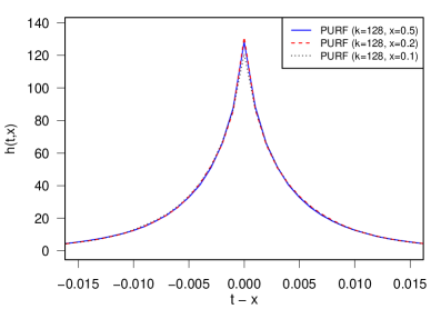
Figure 1: Plot of $\displaystyle h^{\mathcal{U}_{k}^{\mathtt{purf}}}(t,x)$ as a function of $\displaystyle t-x$ for $\displaystyle x\in\left\{\left.0.1,0.2,0.5\right.\right\}$. The values have been estimated by a Monte-Carlo approximation with $\displaystyle 10\,000$ realizations of $\displaystyle\mathbb{U}$.

5.2 Bias for twice differentiable functions

As a corollary of Proposition 3, we get the following estimates of the terms appearing in decomposition (5) of the bias for the PURF model.

Corollary 7.

Let $\displaystyle k\geq 1$, $\displaystyle x\in[0,1)$ and assume (H2a) and (Unif) hold true. Then,

$$\displaystyle 0\leq\mathcal{B}_{\mathcal{U}_{k}^{\mathtt{purf}},\infty}(x) \displaystyle\leq\frac{\left(\left.s^{\prime}(x)\right.\right)^{2}}{2k^{2}}+\frac{2C_{2}^{2}}{k^{4}}$$ (32)

$$\displaystyle\mbox{and}\quad 0\leq\mathcal{V}_{\mathcal{U}_{k}^{\mathtt{purf}}}(x) \displaystyle\leq\frac{\left(\left.s^{\prime}(x)\right.\right)^{2}}{2k^{2}}\enspace.$$ (33)

Let $\displaystyle k\geq 27$ and $\displaystyle\varepsilon^{\mathtt{purf}}_{k}:=\frac{4\log k}{k}$. Then, for every $\displaystyle x\in\left[\left.\varepsilon^{\mathtt{purf}}_{k},1-\varepsilon^{\mathtt{purf}}_{k}\right.\right]$,

$$\displaystyle\mathcal{B}_{\mathcal{U}_{k}^{\mathtt{purf}},\infty}(x) \displaystyle\leq\frac{2C_{2}^{2}}{k^{4}}+\frac{\left(\left.s^{\prime}(x)\right.\right)^{2}}{2k^{6}}$$ (34)

$$\displaystyle\mbox{and}\quad\left\lvert\mathcal{V}_{\mathcal{U}_{k}^{\mathtt{purf}}}(x)-\frac{\left(\left.s^{\prime}(x)\right.\right)^{2}}{2k^{2}}\right\rvert \displaystyle\leq\frac{5}{k^{3}}\left(\left.\left\lvert s^{\prime}(x)\right\rvert+C_{2}\right.\right)^{2}\enspace.$$ (35)

As a consequence, if $\displaystyle k\geq 27$,

$$\displaystyle\int_{0}^{1}\mathcal{B}_{\mathcal{U}_{k}^{\mathtt{purf}},\infty}(x)dx \displaystyle\leq\frac{4\left\lVert s^{\prime}\right\rVert_{\infty}^{2}\log(k)}{k^{3}}+\frac{2C_{2}^{2}}{k^{4}}$$ (36)

$$\displaystyle\int_{\varepsilon^{\mathtt{purf}}_{k}}^{1-\varepsilon^{\mathtt{purf}}_{k}}\mathcal{B}_{\mathcal{U}_{k}^{\mathtt{purf}},\infty}(x)dx \displaystyle\leq\frac{2C_{2}^{2}}{k^{4}}+\frac{\left\lVert s^{\prime}\right\rVert_{\infty}^{2}}{2k^{6}}$$ (37)

$$\displaystyle\mbox{and}\quad\left\lvert\mathcal{V}_{\mathcal{U}_{k}^{\mathtt{purf}}}-\frac{1}{2k^{2}}\int_{0}^{1}\left(\left.s^{\prime}(x)\right.\right)^{2}\,dx\right\rvert \displaystyle\leq\frac{6\left(\left.(\log(k)+1)\left\lVert s^{\prime}\right\rVert_{\infty}^{2}+C_{2}^{2}\right.\right)}{k^{3}}\enspace.$$ (38)

Corollary 7 is proved in Section C.3.

5.3 Discussion: single tree vs. infinite forest

Results of Corollary 7 involve the same rates as in Corollary 5, so, the discussion of Section 4.3 is also valid for the PURF model (with boundaries of size $\displaystyle\varepsilon^{\mathtt{purf}}_{k}$ instead of $\displaystyle\varepsilon^{\mathtt{toy}}$) except for the lower bound of the estimation error when avoiding border effects. However, we conjecture that the result is the same than for the toy model, but solving all technical issues for proving this is beyond the scope of the paper. So, to sum up, for $\displaystyle n$ sufficiently large, we would again have that the infinite forest decreasing rate smaller or equal to the square of the single tree one. This implies that infinite forests would reach the minimax rate of convergence for $\displaystyle C^{2}$ functions whereas single tree does not.

5.4 Tighter bound for three times differentiable functions

When $\displaystyle s$ is smooth enough, the rates obtained in Corollary 7 are tight, as shown by the following corollary of Proposition 3.

Corollary 8.

Let $\displaystyle k\geq 27$ and assume (H3a) and (Unif) hold true. Then, for every $\displaystyle x\in\left[\left.\varepsilon^{\mathtt{purf}}_{k},1-\varepsilon^{\mathtt{purf}}_{k}\right.\right]$,

$$\displaystyle\left\lvert\mathcal{B}_{\mathcal{U},\infty}(x)-\frac{\left(\left.s^{\prime\prime}(x)\right.\right)^{2}}{4k^{4}}\right\rvert\leq\frac{\left(\left.3C_{3}+\frac{1}{27^{2}}\left\lvert s^{\prime}(x)\right\rvert+2\left\lvert s^{\prime\prime}(x)\right\rvert\right.\right)^{2}}{k^{5}}$$ (39)

and for every $\displaystyle x\in(0,1)\backslash\left[\left.\varepsilon^{\mathtt{purf}}_{k},1-\varepsilon^{\mathtt{purf}}_{k}\right.\right]$,

$$\displaystyle\left\lvert\mathcal{B}_{\mathcal{U},\infty}(x)-\frac{\left(\left.s^{\prime}(x)\right.\right)^{2}\left(\left.x^{k+1}-\left(\left.1-x\right.\right)^{k+1}\right.\right)^{2}}{4k^{2}}\right\rvert\leq\frac{\left(\left.C_{3}+\left\lvert s^{\prime}(x)\right\rvert+\left\lvert s^{\prime\prime}(x)\right\rvert\right.\right)^{2}}{2k^{3}}$$ (40)

As a consequence,

$$\displaystyle\left\lvert\int_{0}^{1}\mathcal{B}_{\mathcal{U},\infty}(x)\,dx-\frac{\left(\left.s^{\prime}(0)\right.\right)^{2}+\left(\left.s^{\prime}(1)\right.\right)^{2}}{8k^{3}}\right\rvert\leq\frac{6\left(\left.C_{3}+\left\lVert s^{\prime}\right\rVert_{\infty}+\left\lVert s^{\prime\prime}\right\rVert_{\infty}\right.\right)^{2}\log k}{k^{4}}$$ (41)

$$\displaystyle\mbox{and}\quad\left\lvert\int_{\varepsilon^{\mathtt{purf}}_{k}}^{1-\varepsilon^{\mathtt{purf}}_{k}}\mathcal{B}_{\mathcal{U},\infty}(x)\,dx-\frac{1}{4k^{4}}\int_{0}^{1}\left(\left.s^{\prime\prime}(x)\right.\right)^{2}\,dx\right\rvert\leq\frac{\left(\left.3C_{3}+\frac{1}{27^{2}}\left\lVert s^{\prime}\right\rVert_{\infty}+2\left\lVert s^{\prime\prime}\right\rVert_{\infty}\right.\right)^{2}}{k^{5}}$$ (42)

Corollary 8 is proved in Section C.4. As for the toy model, Corollary 8 implies that under (H3a), a PURF with $\displaystyle q$ trees behaves as the infinite forest as soon as $\displaystyle q\geq k^{2}$.

6 Balanced purely random forests

We consider in this section the following multidimensional PRF model, that we call Balanced Purely Random Forests (BPRF).

6.1 Description of the model

Let $\displaystyle d\geq 1$ be fixed and $\displaystyle\mathcal{X}=[0,1)^{d}$. We define the sequence $\displaystyle(\mathbb{U}_{p})_{p\in\mathbb{N}}$ of random partitions (or random trees) as follows:

• $\displaystyle\mathbb{U}_{0}=[0,1)^{d}$ a.s.

• for every $\displaystyle p\in\mathbb{N}$, given $\displaystyle\mathbb{U}_{p}$, we define $\displaystyle\mathbb{U}_{p+1}$ by splitting each piece $\displaystyle\lambda\in\mathbb{U}_{p}$ into two pieces, where the split is made along some random direction (chosen uniformly over $\displaystyle\left\{\left.1,\ldots,d\right.\right\}$) at some point chosen uniformly.
  Formally, given $\displaystyle\mathbb{U}_{p}=\left\{\left.\lambda_{1,p},\ldots,\lambda_{2^{p},p}\right.\right\}$, let $\displaystyle L_{1,p},\ldots,L_{2^{p},p},Z_{1,p},\ldots,Z_{2^{p},p}$ be independent random variables, independent from $\displaystyle\mathbb{U}_{p}$, such that

  $$\forall j\in\left\{\left.1,\ldots,2^{p}\right.\right\}\,,\quad L_{j,p}\sim\mathcal{U}\left(\left.\left\{\left.1,\ldots,d\right.\right\}\right.\right)\quad\mbox{and}\quad Z_{j,p}\sim\mathcal{U}\left(\left.\left[\left.0,1\right.\right]\right.\right)\enspace.$$

  Then, $\displaystyle\mathbb{U}_{p+1}$ is defined as follows: for every $\displaystyle j\in\left\{\left.1,\ldots,2^{p}\right.\right\}$, $\displaystyle\lambda_{j,p}=\prod_{i=1}^{d}[A_{i},B_{i})$ is split into

  $$\displaystyle\lambda_{2j-1,p+1} \displaystyle=\prod_{i<L_{j,p}}[A_{i},B_{i})\times[A_{L_{j,p}},\left(\left.1-Z_{j,p}\right.\right)A_{L_{j,p}}+Z_{j,p}B_{L_{j,p}})\times\prod_{i>L_{j,p}}[A_{i},B_{i})$$

  $$\displaystyle\mbox{and}\quad\lambda_{2j,p+1} \displaystyle=\prod_{i<L_{j,p}}[A_{i},B_{i})\times[\left(\left.1-Z_{j,p}\right.\right)A_{L_{j,p}}+Z_{j,p}B_{L_{j,p}},B_{L_{j,p}})\times\prod_{i>L_{j,p}}[A_{i},B_{i})\enspace.$$

Then, for every $\displaystyle p\in\mathbb{N}$, we get a random partition $\displaystyle\mathbb{U}_{p}\sim\mathcal{U}_{p}^{\mathtt{bprf}}$ of $\displaystyle\mathcal{X}=[0,1)^{d}$ into $\displaystyle k=2^{p}$ pieces.

This model is very close to the UBPRF model introduced in Breiman, (2000) and theoretically studied by Biau et al., (2008). The only difference is that, at each step all sets of the current partition are split in BPRF, resulting with balanced trees, whereas in UBPRF, only one set (randomly selected with a uniform distribution) of the current partition is split; see also Section 6.4 for a comparison of these two models.

We also point out a similitude between BPRF and another model: Rahimi and Recht, (2008) use $\displaystyle\mathcal{U}_{1}^{\mathtt{bprf}}$ as random partitioning scheme, but without considering the same forest estimator at the end: instead of averaging the tree estimators with uniform weights as we do, Rahimi and Recht, (2008) make a weighted average with data-driven weights.

6.2 Interpretation of the bias of the infinite forest

As in Section 5.1, we can try to interpret the bias of the infinite forest for $\displaystyle\mathcal{U}_{p}^{\mathtt{bprf}}$ as being equal to the bias of an estimator close to a kernel estimator with “kernel function” $\displaystyle h^{\mathcal{U}_{p}^{\mathtt{bprf}}}$ given by Eq. (31). Contrary to the PURF model case, $\displaystyle t-x\mapsto h^{\mathcal{U}_{p}^{\mathtt{bprf}}}(t,x)$ strongly depends on $\displaystyle x$, as shown by the left plot of Figure 2. The right plot of Figure 2 compares $\displaystyle h^{\mathcal{U}}$ with $\displaystyle\mathcal{U}=\mathcal{U}_{p}^{\mathtt{bprf}}$ to $\displaystyle\mathcal{U}\in\left\{\left.\mathcal{U}_{k}^{\mathtt{toy}},\mathcal{U}_{k}^{\mathtt{purf}}\right.\right\}$ for a fixed $\displaystyle x=1/2$ and $\displaystyle k=2^{p}=128$: it turns out that $\displaystyle h^{\mathcal{U}^{\mathtt{toy}}}$ and $\displaystyle h^{\mathcal{U}^{\mathtt{purf}}}$ are the narrowest—$\displaystyle h^{\mathcal{U}^{\mathtt{purf}}}$ appearing as a smooth approximation of $\displaystyle h^{\mathcal{U}^{\mathtt{toy}}}$—whereas $\displaystyle h^{\mathcal{U}^{\mathtt{bprf}}}$ is significantly flatter than the others. This relative flatness can explain the slower rates obtained for the bias of the BPRF model in the next section.

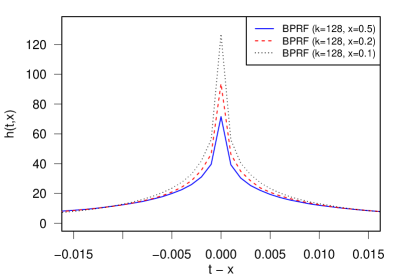
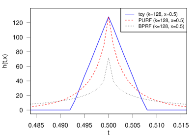
Figure 2: Left: Plot of $\displaystyle h^{\mathcal{U}_{7}^{\mathtt{bprf}}}(t,x)$ as a function of $\displaystyle t-x$ for $\displaystyle x\in\left\{\left.0.1,0.2,0.5\right.\right\}$. Right: Plot of $\displaystyle h^{\mathcal{U}}(t,x)$ with $\displaystyle\mathcal{U}\in\left\{\left.\mathcal{U}_{128}^{\mathtt{toy}},\mathcal{U}_{128}^{\mathtt{purf}},\mathcal{U}_{7}^{\mathtt{bprf}}\right.\right\}$ as a function of $\displaystyle t$ for $\displaystyle x=0.5$. The values have been estimated by a Monte-Carlo approximation with $\displaystyle 10\,000$ realizations of $\displaystyle\mathbb{U}$.

6.3 Bias for twice differentiable functions

As a corollary of Proposition 3, we get the following estimates of the terms appearing in decomposition (5) of the bias for the BPRF model.

Corollary 9.

Let $\displaystyle p\geq 2$ and assume (H2a) and (Unif) hold true. Then, for every $\displaystyle x\in[0,1)^{d}$,

$$\displaystyle\mathcal{B}_{\mathcal{U}_{p}^{\mathtt{bprf}},\infty}(x) \displaystyle\leq\left(\left.1-\frac{1}{2d}\right.\right)^{2p}\left[\left.\frac{1}{2}\left(\left.\nabla s(x)\cdot(1-2x)\right.\right)^{2}+2d^{2}C_{2}^{2}\right.\right]$$ (43)

$$\displaystyle\leq\left(\left.1-\frac{1}{2d}\right.\right)^{2p}\left[\left.\frac{d}{2}\sup_{x\in[0,1)^{d}}\left\lVert\nabla s(x)\right\rVert_{2}^{2}+2d^{2}C_{2}^{2}\right.\right]$$

$$\displaystyle\mbox{and}\qquad\left\lvert\mathcal{V}_{\mathcal{U}_{p}^{\mathtt{bprf}}}(x)-\frac{1}{2}\left(\left.1-\frac{1}{2d}\right.\right)^{p}\sum_{i=1}^{d}\left[\left.\left(\left.\frac{\partial s}{\partial x_{i}}(x)\right.\right)^{2}x_{i}(1-x_{i})\right.\right]\right\rvert$$ (44)

$$\displaystyle\leq\frac{d}{4}\sup_{x\in[0,1)^{d}}\left\lVert\nabla s(x)\right\rVert_{2}^{2}\left(\left.1-\frac{1}{2d}\right.\right)^{2p}$$

$$\displaystyle\qquad+\left[\left.d\max_{1\leq i\leq d}\left(\left.\frac{\partial s}{\partial x_{i}}(x)\right.\right)^{2}+d^{2}\max_{1\leq i\neq j\leq d}\left\lvert\frac{\partial^{2}s}{\partial x_{i}\partial x_{j}}(x)\right\rvert+5dC_{2}^{2}\right.\right]$$

$$\displaystyle\qquad\times\sqrt{\left(\left.1-\frac{1}{2d}\right.\right)^{p}\left(\left.1-\frac{2}{3d}\right.\right)^{p}}\enspace.$$

As a consequence,

$$\displaystyle\int_{[0,1)^{d}}\mathcal{B}_{\mathcal{U}_{p}^{\mathtt{bprf}},\infty}(x)dx \displaystyle\leq\left(\left.1-\frac{1}{2d}\right.\right)^{2p}\left[\left.\frac{1}{2}\int_{[0,1)^{d}}\left(\left.\nabla s(x)\cdot(1-2x)\right.\right)^{2}\,dx+2d^{2}C_{2}^{2}\right.\right]$$ (45)

$$\displaystyle\leq\left(\left.1-\frac{1}{2d}\right.\right)^{2p}\left[\left.\frac{d}{2}\sup_{x\in[0,1)^{d}}\left\lVert\nabla s(x)\right\rVert_{2}^{2}+2d^{2}C_{2}^{2}\right.\right]$$

$$\displaystyle\mbox{and}\qquad\left\lvert\int_{[0,1)^{d}}\mathcal{V}_{\mathcal{U}_{p}^{\mathtt{bprf}}}(x)dx-\frac{1}{2}\left(\left.1-\frac{1}{2d}\right.\right)^{p}\sum_{i=1}^{d}\int_{[0,1)^{d}}\left[\left.\left(\left.\frac{\partial s}{\partial x_{i}}(x)\right.\right)^{2}x_{i}(1-x_{i})\right.\right]\,dx\right\rvert$$

$$\displaystyle\leq\frac{d}{4}\sup_{x\in[0,1)^{d}}\left\lVert\nabla s(x)\right\rVert_{2}^{2}\left(\left.1-\frac{1}{2d}\right.\right)^{2p}$$ (46)

$$\displaystyle\qquad+\sup_{x\in[0,1)^{d}}\left[\left.d\max_{1\leq i\leq d}\left(\left.\frac{\partial s}{\partial x_{i}}(x)\right.\right)^{2}+d^{2}\max_{1\leq i\neq j\leq d}\left\lvert\frac{\partial^{2}s}{\partial x_{i}\partial x_{j}}(x)\right\rvert+5dC_{2}^{2}\right.\right]$$

$$\displaystyle\qquad\times\sqrt{\left(\left.1-\frac{1}{2d}\right.\right)^{p}\left(\left.1-\frac{2}{3d}\right.\right)^{p}}\enspace.$$

Corollary 9 is proved in Section D.4. Remark that contrary to the toy and PURF model, there is no border effect for the approximation error in the BPRF model.

6.4 Discussion: single tree vs. infinite forest

We can now compare a single tree and an infinite forest for the toy model $\displaystyle\mathcal{U}_{p}^{\mathtt{bprf}}$, first in terms of approximation error for a given $\displaystyle p$, then in terms of risk for a well-chosen $\displaystyle p$. In this section, we assume (H2a) and (Unif) hold true.

Approximation error

Let

$$\alpha:=\frac{-\log\left(\left.1-\frac{1}{2d}\right.\right)}{\log(2)}>0$$

be such that

$$k^{-\alpha}=\left(\left.1-\frac{1}{2d}\right.\right)^{p}\quad\mbox{when}\quad k=2^{p}\,.$$

Corollary 9 and Eq. (6) allow to compare the approximation errors of a single tree and of an infinite forest:

$$\mathcal{B}_{\mathcal{U},\infty}\leq L(s,d)k^{-2\alpha}\quad\mbox{whereas}\quad\mathcal{B}_{\mathcal{U},1}\geq L(s,d)k^{-\alpha}-L(s,d)k^{-2\alpha}\enspace.$$ (47)

Therefore, considering an infinite forest instead of a single tree decreases the approximation error from an order of magnitude, and not only from a constant factor when the height of the trees tends to infinity. We emphasize that, as in Section 4.3 and 5.3, we get an infinite forest bias decreasing rate smaller or equal to the square of the single tree one.

Nevertheless, the single tree bias rate is strictly slower than the bias rate of a classical regular partitioning estimate (with a cubic partition in $\displaystyle k$ sets), which is $\displaystyle k^{-2/d}$ (see e.g. Chapter 4 in Györfi et al.,, 2002). Indeed, we have that for all $\displaystyle d\geq 1$,

$$\alpha\leq\frac{1}{2\log(2)d}<\frac{2}{d}$$

since $\displaystyle\log(1+u)\leq u$ for all $\displaystyle u>-1$.

Risk bounds for a well-chosen $\displaystyle p$

The above controls on the approximation errors imply controls on the statistical risk of the estimators built on a single tree and on an infinite forest, respectively. Indeed, for all $\displaystyle q\in[1,+\infty]$, if $\displaystyle n\geq 1$ data points are available, the statistical risk of the estimator built upon a random forest of $\displaystyle q$ trees with $\displaystyle k=2^{p}\geq 2$ leaves can be bounded by Eq. (4) and Proposition 2. In order to apply Proposition 2, we need the following lemma.

Lemma 10.

Let $\displaystyle p\geq 0$. Then,

$$\mathbb{E}_{\mathbb{U}\sim\mathcal{U}_{p}^{\mathtt{bprf}}}\left[\left.\sum_{\lambda\in\mathbb{U}}\left(\left.\operatorname{diam}_{L^{2}}(\lambda)\right.\right)^{2}\right.\right]=2^{p}\left(\left.1-\frac{2}{3d}\right.\right)^{p}$$ (48)

and for every $\displaystyle u>0$,

$$\mathbb{E}_{\mathbb{U}\sim\mathcal{U}_{p}^{\mathtt{bprf}}}\left[\left.\sum_{\lambda\in\mathbb{U}}\exp\left(\left.-n|\lambda|\right.\right)\right.\right]\leq 2^{p}\left[\left.\frac{1}{u}+\left(\left.1-\frac{1}{u}\right.\right)\exp\left(\left.-ne^{-\left(\left.p+\sqrt{up}\right.\right)}\right.\right)\right.\right]\enspace.$$ (49)

In particular, if $\displaystyle n\geq\exp\left(\left.p+\sqrt{5p}\right.\right)$,

$$\mathbb{E}_{\mathbb{U}\sim\mathcal{U}_{p}^{\mathtt{bprf}}}\left[\left.\sum_{\lambda\in\mathbb{U}}\exp\left(\left.-n|\lambda|\right.\right)\right.\right]\leq 2^{p}\kappa\quad\mbox{where}\quad\kappa:=\frac{1+4e^{-1}}{5}<\frac{1}{2}\enspace.$$ (50)

Lemma 10 is proved in Section D.6. The proof of Lemma 10 in Section D.6 also shows the volume of each element of a partition $\displaystyle\mathbb{U}\sim\mathcal{U}_{p}^{\mathtt{bprf}}$ is typically of order $\displaystyle\exp\left(\left.-p\pm L\sqrt{p}\right.\right)$, so it is hopeless to consider values of $\displaystyle p$ such that this typical volume is smaller than $\displaystyle 1/n$. Hence, throughout this subsection, for comparing risks with a well-chosen $\displaystyle p$, we only consider values of $\displaystyle p$ such that

$$n\geq\exp\left(\left.p+\sqrt{5p}\right.\right)\quad\Leftrightarrow\quad p\leq\left(\left.\sqrt{\frac{5}{4}+\log n}-\frac{\sqrt{5}}{2}\right.\right)^{2}\enspace.$$ (51)

Remark that under assumption (H2a), $\displaystyle s$ is $\displaystyle K$-Lipschitz with respect to the $\displaystyle L^{2}$ distance on $\displaystyle\mathcal{X}$ with $\displaystyle K=\sup_{x\in\mathcal{X}}\left\lVert\nabla s(x)\right\rVert_{2}=\left\lVert\nabla s\right\rVert_{\infty,2}$. So, Proposition 2 shows that for the BPRF model with trees having $\displaystyle k=2^{p}$ leaves, if $\displaystyle n\geq 1$ data points are available and if Eq. (51) holds true,

$$\displaystyle\mathbb{E}\left[\left.\left(\left.\widehat{s}_{\infty}\left(\left.X;D_{n}\right.\right)-s(X)\right.\right)^{2}\right.\right] \displaystyle\leq\mathcal{B}_{\mathcal{U}_{p}^{\mathtt{bprf}},\infty}+\frac{2\sigma^{2}k}{n}+\frac{2\left\lVert\nabla s\right\rVert_{\infty,2}^{2}}{nk^{\beta}}+\frac{\left\lVert s\right\rVert_{\infty}^{2}k}{n}\left[\left.\frac{1}{u}+\exp\left(\left.-nk^{-(1+\sqrt{u/p})/\log 2}\right.\right)\right.\right]$$

for every $\displaystyle u\geq 1$, where

$$\beta:=\frac{-\log\left(\left.2\left(\left.1-\frac{2}{3d}\right.\right)\right.\right)}{\log(2)}\enspace.$$

So, since $\displaystyle\mathcal{B}_{\mathcal{U}_{p}^{\mathtt{bprf}},\infty}\leq L(s,d)k^{-2\alpha}$, if we are able to choose the number of leaves $\displaystyle k=2^{p}$ optimally (with an estimator selection procedure, such as cross-validation), the risk of the infinite forest estimator is upper bounded as follows:

$$\displaystyle\qquad\mathbb{E}\left[\left.\left(\left.\widehat{s}_{\infty}\left(\left.X;D_{n}\right.\right)-s(X)\right.\right)^{2}\right.\right]$$

$$\displaystyle\leq L(s,d)\inf_{u\geq 1,\,k=2^{p},\,0\leq p\leq\left(\left.\sqrt{\frac{5}{4}+\log n}-\frac{\sqrt{5}}{2}\right.\right)^{2}}\left\{\left.k^{-2\alpha}+\frac{\sigma^{2}k}{n}+\frac{1}{nk^{\beta}}+\frac{k}{n}\left[\left.\frac{1}{u}+\exp\left(\left.-nk^{-(1+\sqrt{u/p})/\log 2}\right.\right)\right.\right]\right.\right\}\enspace.$$ (52)

Now, for upper bounding the infimum, two cases must be distinguished: (i) when $\displaystyle d\leq 3$, so that $\displaystyle 1/(1+2\alpha)<\log 2$, and (ii) when $\displaystyle d\geq 4$, so that $\displaystyle 1/(1+2\alpha)>\log 2$.

In case (i), some nonnegative integer $\displaystyle p^{*}\leq\left(\left.\sqrt{\frac{5}{4}+\log n}-\frac{\sqrt{5}}{2}\right.\right)^{2}$ exists such that

$$k^{*}=2^{p^{*}}\in\left[\left.\left(\left.\frac{n}{\sigma^{2}}\right.\right)^{1/(1+2\alpha)},2\left(\left.\frac{n}{\sigma^{2}}\right.\right)^{1/(1+2\alpha)}\right.\right]$$

if $\displaystyle n\geq L(\sigma^{2})$. Since $\displaystyle\alpha\geq\log(6/5)/\log(2)>(1/\log(2)-1)/2$, for some (small enough) numerical constants $\displaystyle\delta_{1},\delta_{2}>0$, if $\displaystyle n\geq L(\sigma^{2})$,

$$nk^{*\,-\frac{1+\delta_{1}}{\log 2}}\geq Ln\left(\left.\frac{n}{\sigma^{2}}\right.\right)^{-\frac{1+\delta_{1}}{(1+2\alpha)\log(2)}}\geq n^{\delta_{2}}\enspace,$$

taking $\displaystyle u=\delta_{1}^{2}p^{*}$ in Eq. (52) yields

$$\displaystyle\qquad\mathbb{E}\left[\left.\left(\left.\widehat{s}_{\infty}\left(\left.X;D_{n}\right.\right)-s(X)\right.\right)^{2}\right.\right]$$ (53)

$$\displaystyle\leq L(s,d)\left[\left.\left(\left.\frac{\sigma^{2}}{n}\right.\right)^{\frac{2\alpha}{2\alpha+1}}+L(\sigma^{2})n^{-\frac{2\alpha}{2\alpha+1}}\left[\left.\frac{1}{\delta_{1}^{2}p^{*}}+\exp\left(\left.-n^{\delta_{2}}\right.\right)\right.\right]\right.\right]$$

$$\displaystyle\leq L(s,d)\left(\left.\frac{\sigma^{2}}{n}\right.\right)^{\frac{2\alpha}{2\alpha+1}}$$

as soon as $\displaystyle n\geq L(\sigma^{2})$.

In case (ii), a similar reasoning with some integer

$$p^{*}\in\left(\left(\left.\sqrt{\frac{5}{4}+\log n}-\frac{\sqrt{5}}{2}\right.\right)^{2}-1,\left(\left.\sqrt{\frac{5}{4}+\log n}-\frac{\sqrt{5}}{2}\right.\right)^{2}\right]$$

yields

$$\displaystyle\mathbb{E}\left[\left.\left(\left.\widehat{s}_{\infty}\left(\left.X;D_{n}\right.\right)-s(X)\right.\right)^{2}\right.\right] \displaystyle\leq L(s,d,\sigma^{2})n^{-2\alpha\log 2}2^{2\alpha\sqrt{5}\sqrt{\log n+\frac{5}{4}}}\enspace.$$

In particular, we get a rate of order $\displaystyle n^{-(2\alpha\log 2-\delta)}$ for every $\displaystyle\delta>0$, which is slightly worse than the rate $\displaystyle n^{-2\alpha/(2\alpha+1)}$ for $\displaystyle d\geq 4$ since $\displaystyle\log 2\leq 1/(1+2\alpha)$.

For lower bounding the risk of a single tree, we apply Eq. (9) in Proposition 2. By Eq. (47), if $\displaystyle p\geq p_{0}=L(s,d)$ and $\displaystyle k=2^{p}$,

$$\mathcal{B}_{\mathcal{U}_{p}^{\mathtt{bprf}},1}\geq L(s,d)k^{-\alpha}-L(s,d)k^{-2\alpha}\geq L(s,d)k^{-\alpha}$$

so that Eq. (4), Proposition 2 and Eq. (50) in Lemma 10 imply, if $\displaystyle\mathbb{U}\sim\mathcal{U}_{p}^{\mathtt{bprf}}$ with $\displaystyle p_{0}\leq p\leq\left(\left.\sqrt{\frac{5}{4}+\log n}-\frac{\sqrt{5}}{2}\right.\right)^{2}$,

$$\displaystyle\mathbb{E}\left[\left.\left(\left.\widehat{s}\left(\left.X;\mathbb{U};D_{n}\right.\right)-s(X)\right.\right)^{2}\right.\right] \displaystyle\geq\inf_{k=2^{p},p_{0}\leq p\leq\left(\left.\sqrt{\frac{5}{4}+\log n}-\frac{\sqrt{5}}{2}\right.\right)^{2}}\left\{\left.L(s,d)k^{-\alpha}+\frac{\sigma^{2}k\left(\left.1-2\kappa\right.\right)}{n}\right.\right\}\enspace.$$ (54)

Here, again, we must distinguish the cases (i) $\displaystyle d\leq 3$ and (ii) $\displaystyle d\geq 4$. If $\displaystyle d\leq 3$, by Lemma 20, Eq. (54) shows that if in addition $\displaystyle n\geq L(d,\sigma^{2})$,

$$\displaystyle\mathbb{E}\left[\left.\left(\left.\widehat{s}\left(\left.X;\mathbb{U};D_{n}\right.\right)-s(X)\right.\right)^{2}\right.\right] \displaystyle\geq L(s,d)\left(\left.\frac{\sigma^{2}}{n}\right.\right)^{\alpha/(\alpha+1)}\enspace.$$

If $\displaystyle d\geq 4$, Eq. (54) shows that

$$\displaystyle\mathbb{E}\left[\left.\left(\left.\widehat{s}\left(\left.X;\mathbb{U};D_{n}\right.\right)-s(X)\right.\right)^{2}\right.\right] \displaystyle\geq L(s,d)\inf_{0\leq k\leq 2^{5/2}n^{\log(2)}}\left\{\left.k^{-\alpha}+\frac{\sigma^{2}k}{n}\right.\right\}$$

$$\displaystyle\geq L(s,d)n^{-\alpha\log(2)}$$

for $\displaystyle n\geq L(\sigma^{2},d)$, since the function $\displaystyle x\to x^{-\alpha}+\frac{\sigma^{2}x}{n}$ is then decreasing on $\displaystyle(0,(n\alpha/\sigma^{2})^{1/(\alpha+1)}]$ and

$$\frac{1}{\alpha+1}\geq\frac{1}{1+\frac{\log(8/7)}{\log(2)}}>\log(2)\enspace.$$

So, in both cases ($\displaystyle d\leq 3$ or $\displaystyle d\geq 4$), the infinite forest has a faster rate of convergence (in terms of risk) than a single tree. But, even with an infinite forest with $\displaystyle d\leq 3$, since

$$\frac{2\alpha}{2\alpha+1}\leq\frac{1}{1+2\log(2)d}<\frac{4}{4+d}\enspace,$$

the rate obtained is slower than the minimax rate $\displaystyle n^{-4/(d+4)}$ over the set of $\displaystyle C^{2}$ functions (see e.g. Györfi et al.,, 2002).

Intuitively, the BPRF model is not minimax because it is not adaptive enough. Indeed, the partitioning process splits each set of the current partition regardless of its size: so a relatively small set is still split the same number of times than a relatively large set. We conjecture that a partitioning scheme with a random choice of the next set to be split, with a probability of choosing each set proportional to its size—as in the PURF model, see Section 1.1—, would be better and could reach the minimax rate for $\displaystyle C^{2}$ functions. This is proved for $\displaystyle d=1$ in Section 5.

Finally, we note that the UBPRF model 2 would certainly suffer from the same lack of adaptivity because the next set to be split is chosen with a uniform distribution on all sets. So, this model would certainly not be minimax either, and we conjecture that it would be even worse than the BPRF model.

6.5 Tighter bound for three times differentiable functions

The bounds in Corollary 9 are tight when $\displaystyle s$ is smooth enough, as shown by the following corollary of Proposition 3.

Corollary 11.

Let $\displaystyle p\geq 2$ and assume (H3a) and (Unif) hold true. Then, for every $\displaystyle x\in[0,1)^{d}$,

$$\begin{split}&\quad\left\lvert\mathcal{B}_{\mathcal{U}_{p}^{\mathtt{bprf}},\infty}(x)-\frac{1}{4}\left(\left.1-\frac{1}{2d}\right.\right)^{2p}\left(\left.\nabla s(x)\cdot(1-2x)+\sum_{i=1}^{d}\left[\left.\frac{\partial^{2}s}{\partial x_{i}^{2}}(x)x_{i}(1-x_{i})\right.\right]\right.\right)^{2}\right\rvert\\ &\leq 6d^{4}\left(\left.1-\frac{2}{3d}\right.\right)^{3p/4}\left(\left.1-\frac{1}{2d}\right.\right)^{p}\left(\left.\left\lVert\nabla s(x)\right\rVert_{2}^{2}+\max_{i,j}\left(\left.\frac{\partial^{2}s}{\partial x_{i}\partial x_{j}}(x)\right.\right)^{2}+C_{3}^{2}\right.\right)\enspace.\end{split}$$ (55)

As a consequence,

$$\begin{split}&\left\lvert\int_{[0,1)^{d}}\mathcal{B}_{\mathcal{U}_{p}^{\mathtt{bprf}},\infty}(x)\,dx-\frac{1}{4}\left(\left.1-\frac{1}{2d}\right.\right)^{2p}\int_{[0,1)^{d}}\left(\left.\nabla s(x)\cdot(1-2x)+\sum_{i=1}^{d}\left[\left.\frac{\partial^{2}s}{\partial x_{i}^{2}}(x)x_{i}(1-x_{i})\right.\right]\right.\right)^{2}\,dx\right\rvert\\ &\leq 6d^{4}\left(\left.1-\frac{2}{3d}\right.\right)^{3p/4}\left(\left.1-\frac{1}{2d}\right.\right)^{p}\left(\left.\sup_{x\in[0,1)^{d}}\left\lVert\nabla s(x)\right\rVert_{2}^{2}+\sup_{x\in[0,1)^{d}}\max_{i,j}\left(\left.\frac{\partial^{2}s}{\partial x_{i}\partial x_{j}}(x)\right.\right)^{2}+C_{3}^{2}\right.\right)\enspace.\end{split}$$ (56)

Corollary 11 is proved in Section D.5.

6.6 Size of the forest

As for the previous models, under (H3a), Corollary 11 and Eq. (2) show a BPRF forest of size $\displaystyle q$ has an approximation error of the same order of magnitude as an infinite forest when

$$q\geq k^{\alpha}=2^{\alpha p}=\left(\left.1-\frac{1}{2d}\right.\right)^{-p}\,.$$

7 Simulation experiments

In order to illustrate mathematical results from previous sections, we lead some simulation experiments with R (R Core Team,, 2014), focusing on approximation errors, as defined in Section 2.3. We consider the models from Sections 4–6 (toy, PURF, BPRF), with $\displaystyle d=1$ for toy and PURF, and $\displaystyle d\in\{1,5,10\}$ for BPRF. In addition, we consider a PRF model discussed in Section 3 of Biau, (2012), that we call Hold-out RF in the following. Hold-out RF is the original RF model 1 except that the tree partitioning is performed using an extra sample $\displaystyle D_{n}^{\prime}$, independent from the learning sample $\displaystyle D_{n}$. As a consequence, assumption ($\displaystyle\mathbf{PR}$) holds for the Hold-out RF model, so decomposition (3) is valid and we can compute the corresponding approximation error, as a function of the number $\displaystyle q$ of trees in the forest.

7.1 Framework

For all experiments, we take the input space $\displaystyle\mathcal{X}=[0,1)^{d}$ and suppose that (Unif) holds. We choose the following regression functions:

• sinusoidal (if $\displaystyle d=1$): $\displaystyle x\mapsto\sin(2\pi x)$,

• absolute value (if $\displaystyle d=1$): $\displaystyle x\mapsto\left\lvert x-\frac{1}{2}\right\rvert$,

• sum (for any $\displaystyle d\geq 1$): $\displaystyle x\mapsto\sum_{j=1}^{d}x_{j}$,

• Friedman1 (for any $\displaystyle d\geq 5$):

  $$x\mapsto\textbf{1/10}\times\left[\left.10\sin(\pi x_{1}x_{2})+20(x_{3}-0.5)^{2}+10x_{4}+5x_{5}\right.\right]$$

  which is proportional to the Friedman1 function that was introduced by Friedman, (1991). Here we add the scaling factor $\displaystyle 1/10$ in order to have a function with a range comparable to that of sum.

For all PRF models, we choose $\displaystyle k$, the number of leaves (minus one for toy and PURF), among $\displaystyle\left\{\left.2^{5},2^{6},2^{7},2^{8},2^{9}\right.\right\}$; the last value $\displaystyle 2^{9}$ is sometimes removed for computational reasons.

Quantities $\displaystyle\mathcal{B}_{\mathcal{U},1}$ and $\displaystyle\mathcal{B}_{\mathcal{U},\infty}$ are estimated by Monte-Carlo approximation using:

• $\displaystyle 1000$ realizations of $\displaystyle X$,

• for $\displaystyle\mathcal{B}_{\mathcal{U},1}$, $\displaystyle 500$ realizations of $\displaystyle\mathbb{U}$,

• for $\displaystyle\mathcal{B}_{\mathcal{U},\infty}$, $\displaystyle k^{2}$ realizations of $\displaystyle\mathbb{U}$ for toy and PURF models, $\displaystyle k^{2\alpha}$ realizations for BPRF model with $\displaystyle\alpha=-\log(1-1/(2d))/\log(2)$ (which ensures our estimation of the convergence rates is precise enough, according to our theoretical results), and $\displaystyle k^{2}$ realizations for Hold-out RF model, which empirically appears to be sufficient for estimating the convergence rates correctly for this RF model.

Furthermore, for each computation of $\displaystyle\mathcal{B}_{\mathcal{U},1}$ and $\displaystyle\mathcal{B}_{\mathcal{U},\infty}$ we add some “borderless” estimations of the bias, that is, integrating only over $\displaystyle x\in[\epsilon,1-\epsilon]$ with $\displaystyle\epsilon=\varepsilon^{\mathtt{toy}}_{k}$ or $\displaystyle\varepsilon^{\mathtt{purf}}_{k}$ depending on the model.

In addition, for the Hold-out RF model:

• we simulate the $\displaystyle D_{n}^{\prime}$ sample with $\displaystyle n=k^{2}$ (for each value of $\displaystyle k$) and choose a gaussian random noise with variance $\displaystyle\sigma^{2}=1/16$,

• we use the randomForest R package (Liaw and Wiener,, 2002) to build the trees on the sample $\displaystyle D_{n}^{\prime}$: we use parameters maxnodes (to control the number of leaves) and ntree (to set the number of trees), and take the default values for all other parameters (in particular mtry).

Finally, for each scenario, we plot the bias as a function of $\displaystyle k$ in $\displaystyle\log_{2}$-$\displaystyle\log_{2}$ scale, and estimate the slope of the plot by fitting a simple linear model in order to get an approximation of the convergence rates.

7.2 One-dimensional input space

We consider in this subsection the one-dimensional case ($\displaystyle d=1$). Figure 3 shows results for the sinusoidal regression function.

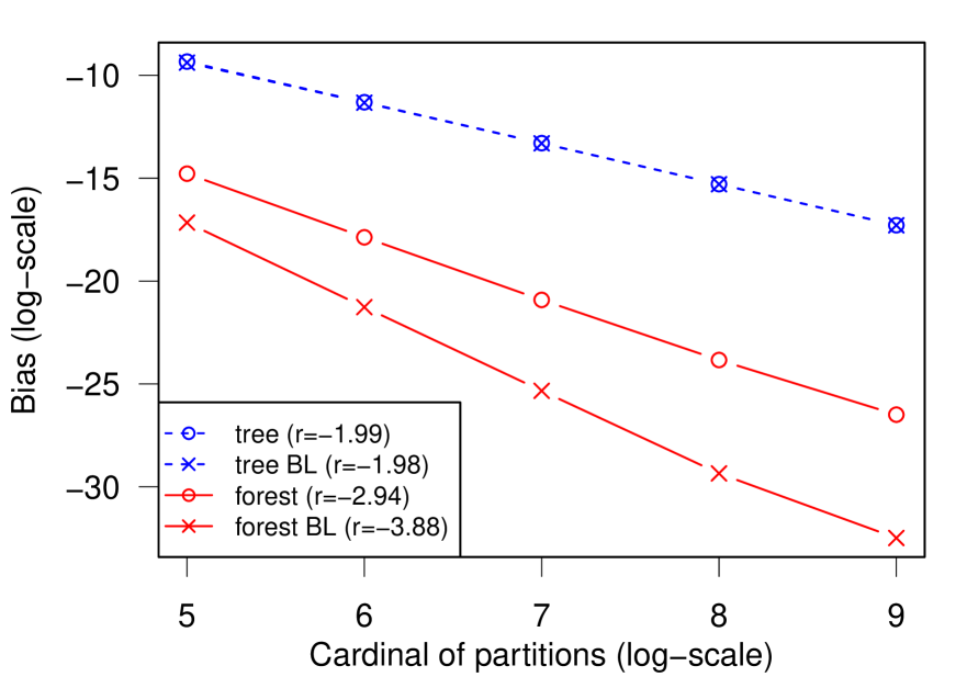
(a) toy, $\displaystyle d=1$

(b) PURF, $\displaystyle d=1$

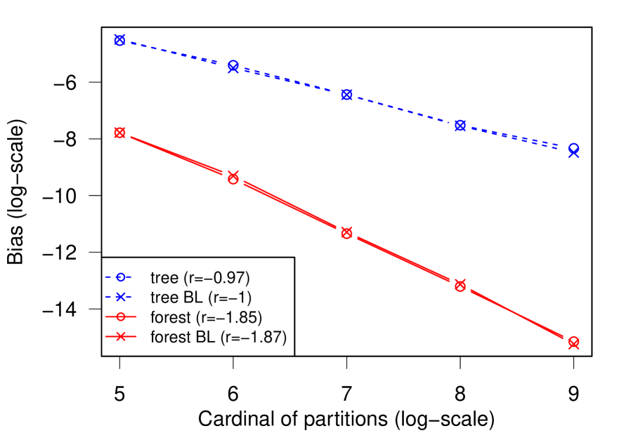
(c) BPRF, $\displaystyle d=1$

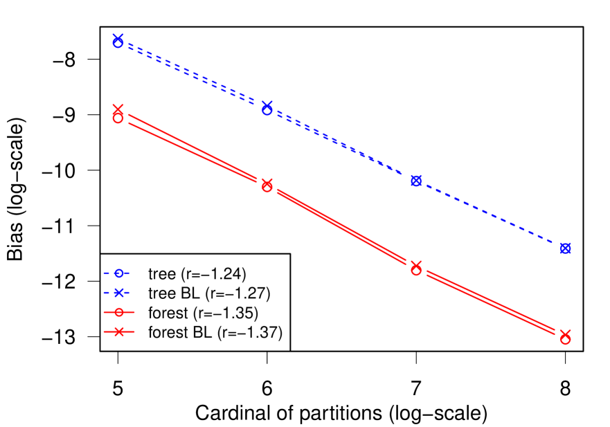
(d) Hold-out RF, $\displaystyle d=1$

Figure 3: Plot of $\displaystyle\mathcal{B}_{\mathcal{U},1}$ and $\displaystyle\mathcal{B}_{\mathcal{U},\infty}$ (in $\displaystyle\log_{2}$-scale) against $\displaystyle k$ (in $\displaystyle\log_{2}$-scale) for (a) toy, (b) PURF, (c) BPRF and (d) Hold-out RF models, for the sinusoidal regression function. BL corresponds to borderless situations and $\displaystyle r$ denotes the slope of a linear model fitted to the scatter plot.

Plots are in $\displaystyle\log_{2}$-$\displaystyle\log_{2}$ scale, so as expected we obtain linear behaviors. For toy and PURF models (top graphs) we get decreasing rates very close to what can be expected from Sections 4–5: $\displaystyle k^{-2}$ for trees (with or without borders), $\displaystyle k^{-3}$ for forests and $\displaystyle k^{-4}$ for borderless forests. Similarly, we get the right decreasing rates for BPRF model (bottom left graph): indeed, if $\displaystyle d=1$ then $\displaystyle\alpha=1$, so trees and forests rates are respectively $\displaystyle k^{-1}$ and $\displaystyle k^{-2}$. For Hold-out RF model we get rates about $\displaystyle k^{-1.25}$ for trees and $\displaystyle k^{-1.35}$ for forests as expected from Section 6. These rates are surprisingly slow (in particular compared to toy and PURF models) and a forest does not bring much improvement compared to a single tree. But as shown in the next section, the one-dimensional case is not the best framework for the Hold-Out-RF model compared to other PRF models.

Results for the absolute value regression function are presented in Figure 4.

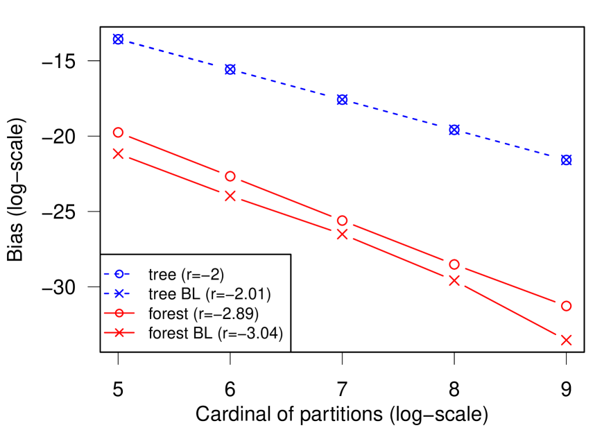
(a) toy, $\displaystyle d=1$

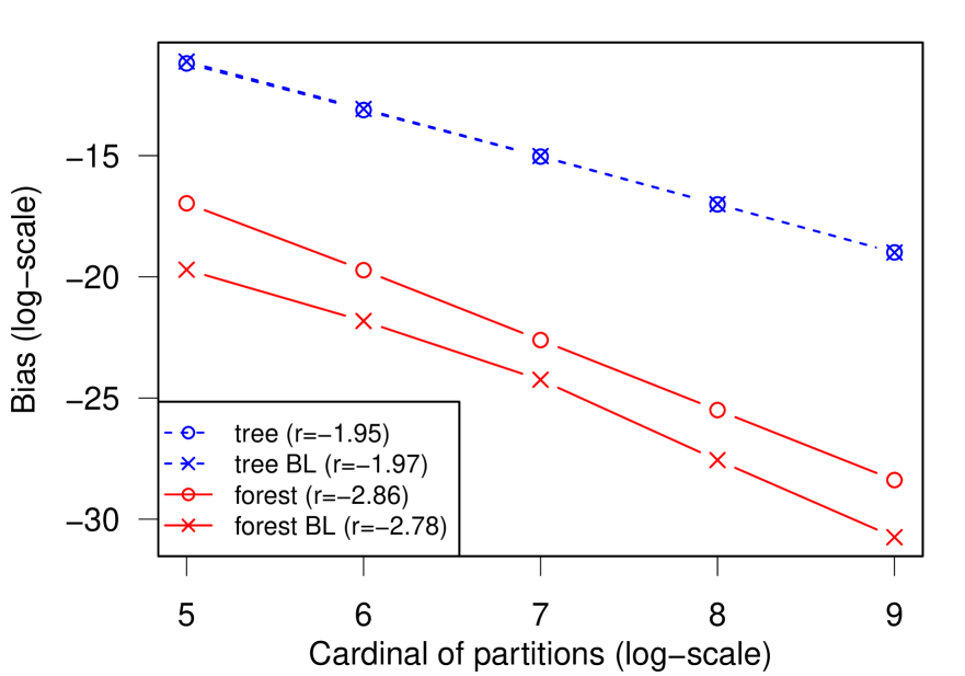
(b) PURF, $\displaystyle d=1$

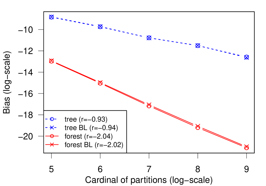
(c) BPRF, $\displaystyle d=1$

(d) Hold-out RF, $\displaystyle d=1$

Figure 4: Plot of $\displaystyle\mathcal{B}_{\mathcal{U},1}$ and $\displaystyle\mathcal{B}_{\mathcal{U},\infty}$ (in $\displaystyle\log_{2}$-scale) against $\displaystyle k$ (in $\displaystyle\log_{2}$-scale) for (a) toy, (b) PURF, (c) BPRF and (d) Hold-out RF models, for the absolute value regression function. BL corresponds to borderless situations and $\displaystyle r$ denotes the slope of a linear model fitted to the scatter plot.

The absolute value regression function presents a singularity at point $\displaystyle x=1/2$, and it acts as a border point. Hence, compared to the sinusoidal regression function, the only change is that there is no differences between borderless and regular approximation errors of forests: both reach the rate $\displaystyle k^{-3}$ for toy and PURF models. The Hold-out RF model again reaches relatively poor rates, and the forest does not improve significantly the bias compared to a single tree.

7.3 Multidimensional input space

For $\displaystyle d>1$, we investigate the behaviors of BPRF and Hold-out RF models. First, Figure 5 shows the results for the sum regression function when $\displaystyle d\in\{5,10\}$.

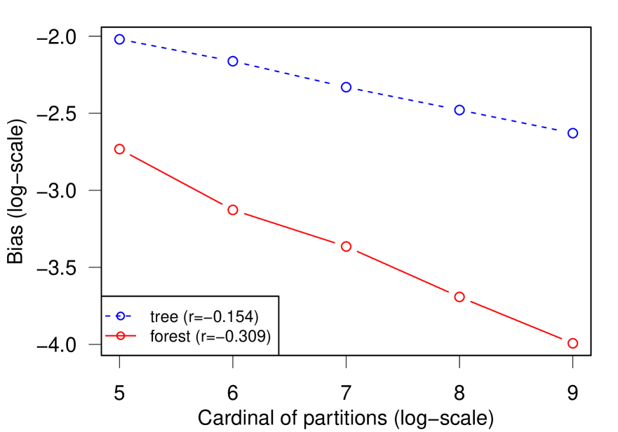
(a) BPRF, $\displaystyle d=5$

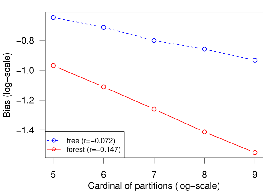
(b) BPRF, $\displaystyle d=10$

(c) Hold-out RF, $\displaystyle d=5$

(d) Hold-out RF, $\displaystyle d=10$

Figure 5: Plot of $\displaystyle\mathcal{B}_{\mathcal{U},1}$ and $\displaystyle\mathcal{B}_{\mathcal{U},\infty}$ (in $\displaystyle\log_{2}$-scale) against $\displaystyle k$ (in $\displaystyle\log_{2}$-scale) for BPRF with (a) $\displaystyle d=5$ and (b) $\displaystyle d=10$, and Hold-out RF model with (c) $\displaystyle d=5$ and (d) $\displaystyle d=10$, for the sum regression function. $\displaystyle r$ denotes the slope of a linear model fitted to the scatter plot.

As in the one-dimensional case, we observe linear behaviors in $\displaystyle\log_{2}$-$\displaystyle\log_{2}$ scale. For BPRF (top graphs), trees and forests reach approximately the decreasing rates we can expect from Section 6, respectively $\displaystyle k^{-\alpha}$ and $\displaystyle k^{-2\alpha}$ with $\displaystyle\alpha=\log(10/9)/\log(2)\approx 0.152$ when $\displaystyle d=5$ and $\displaystyle\alpha=\log(20/19)/\log(2)\approx 0.074$ when $\displaystyle d=10$.

Compared to BPRF, the Hold-out RF model reaches better rates in the multidimensional framework. Moreover, it suffers less from the increase of the dimension: BPRF rates are divided by $\displaystyle 2.1$ when $\displaystyle d$ increases from $\displaystyle 5$ to $\displaystyle 10$, whereas Hold-out RF model rates are only divided by $\displaystyle 1.3$.

Forests rates with the Hold-out RF model are about $\displaystyle 1.6$ times faster than tree rates, which illustrates a significant gain brought by forests. Note however the comparison with BPRF model is partly unfair, because Hold-out RF can make use of an extra sample $\displaystyle D_{n}^{\prime}$ for building appropriate partitions of $\displaystyle\mathcal{X}$; nevertheless, with BPRF, if such an extra sample is available, it can only be used for reducing the final risk by a constant factor (since it doubles the sample size) but not for improving the risk rate.

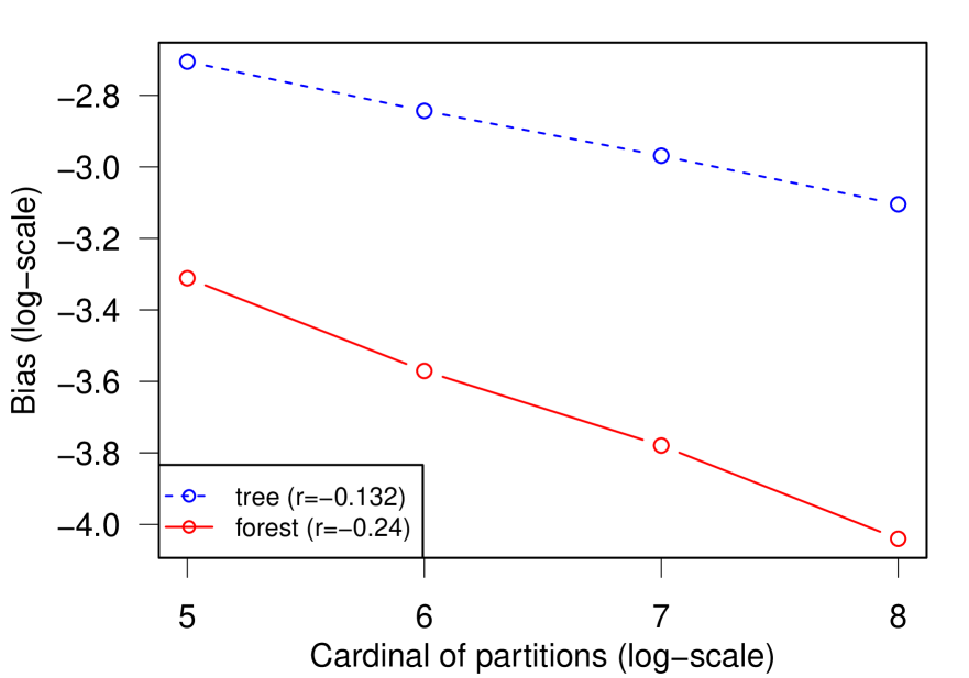
(a) BPRF, $\displaystyle d=5$

(b) BPRF, $\displaystyle d=10$

(c) Hold-out RF, $\displaystyle d=5$

(d) Hold-out RF, $\displaystyle d=10$

Figure 6: Plot of $\displaystyle\mathcal{B}_{\mathcal{U},1}$ and $\displaystyle\mathcal{B}_{\mathcal{U},\infty}$ (in $\displaystyle\log_{2}$-scale) against $\displaystyle k$ (in $\displaystyle\log_{2}$-scale) for BPRF with (a) $\displaystyle d=5$ and (b) $\displaystyle d=10$, and Hold-out RF model with (c) $\displaystyle d=5$ and (d) $\displaystyle d=10$, for the Friedman1 regression function. $\displaystyle r$ denotes the slope of a linear model fitted to the scatter plot.

Results for the Friedman1 regression function are shown in Figure 6. Note that when $\displaystyle d=10$, the last five variables are non-informative since the regression function does not depend on them.

For BPRF, rates are slightly worse than for sum, and we still observe a factor of $\displaystyle 2$ between trees and forests rates. The decrease of the rates might be explained by two reasons: the complexity of Friedman1 function, and when $\displaystyle d=10$ the presence of five non-informative variables.

For the Hold-out RF model, rates are still much better than for BPRF, and forest rates are better than tree rates by a factor $\displaystyle 1.5$. When $\displaystyle d=5$, rates are smaller than for the sum regression function, probably due to the complexity of the regression function. When $\displaystyle d=10$, we surprisingly get faster rates than when $\displaystyle d=5$. Obtaining approximation rates as good for $\displaystyle d=10$ as for $\displaystyle d=5$ is expected since the number of informative variables is the same in both cases, and Hold-out RF are known to adapt to the sparsity of the regression function (see Section 8.1 for more details). But obtaining significantly better rates for a more difficult problem (when $\displaystyle d=10$) is quite surprising. Investigating this phenomenon requires a more systematic simulation study with more examples, which is out of the scope of the present paper.

8 Discussion

In this paper, we analyze several purely random forests models and show, for each of them, that an infinite forest improves by an order of magnitude the approximation error of a single tree, assuming the regression function is smooth. Since the estimation error of a forest is smaller or equal to that of a single tree, we deduce that forests reach a strictly better risk convergence rate.

8.1 Comparison between the toy, PURF and BPRF models

In dimension $\displaystyle d=1$, we can compare the results for the BPRF model in Section 6 with the results obtained in Sections 4 and 5 for the toy and PURF models. Indeed, we get

$$\alpha=1$$

so that the approximation error of an infinite forest is of order $\displaystyle k^{-2}$ for BPRF, instead of $\displaystyle k^{-4}$ for toy and PURF (when avoiding border effects).

Intuitively, it seems the BPRF model tends to leave large “holes” in the space $\displaystyle\mathcal{X}$, whereas the toy model is almost regular, and the PURF model stays close to regular. Recall the PURF model can be seen as a recursive tree construction, where only one leaf is split into two leaves at each step, and the choice of this leaf is made with probability equal to its size. On the contrary, the BPRF model keeps splitting all leaves whatever their size, which may lead to very small leaves but also to much larger ones in some significant part of the space $\displaystyle\mathcal{X}$.

8.2 Comparison with other random forest models

Another random forest model has been suggested by Breiman, (2004) and was more precisely analyzed by Biau, (2012). In the latter paper, the random partitioning—which depends on some parameters $\displaystyle(p_{i})_{1\leq i\leq d}\in[0,1)^{d}$ with $\displaystyle p_{1}+\cdots+p_{d}=1$—is as follows:

Model 4.

• Start from $\displaystyle[0,1)^{d}$,

• Repeat $\displaystyle k$ times: for each set $\displaystyle\lambda$ of the current partition,

  • choose a split variable $\displaystyle j$ randomly, with probability distribution over $\displaystyle\{1,\ldots,d\}$ given by $\displaystyle(p_{i})_{1\leq i\leq d}$,

  • split $\displaystyle\lambda$ along coordinate $\displaystyle j$ at the midpoint $\displaystyle t_{j}$ of $\displaystyle\lambda_{j}$, that is put $\displaystyle\{x\in\lambda\,/\,x_{j}<t_{j}\}$ and $\displaystyle\{x\in\lambda\,/\,x_{j}\geq t_{j}\}$ at the two children nodes below $\displaystyle\lambda$.

In a framework where only $\displaystyle S$ variables (among $\displaystyle d$) are “strong” (i.e. have an effect on the output variable), the main result of Biau, (2012) is that if the probability weights are well tuned (i.e., roughly, if $\displaystyle p_{j}\approx 1/S$ for a strong variable and $\displaystyle p_{j}\approx 0$ for a noisy variable), then for model 4, the infinite forest rate of convergence only depends on $\displaystyle S$ and is faster than the minimax rate in dimension $\displaystyle d$. In other words, Biau, (2012) shows that such random forests adapt to sparsity.

Even if the framework of Biau, (2012) is quite different from ours, let us give a quick comparison between the different rates obtained when $\displaystyle S=d$. Assuming the regression function is Lipschitz, for the model studied by Biau, (2012), the infinite forest bias is at most of order $\displaystyle k^{-\theta}$ with $\displaystyle\theta=3/(4\log(2)d)$. This is comparable to our result $\displaystyle k^{-2\alpha}$ for BPRF, because $\displaystyle 2\alpha\approx 1/(\log(2)d)$ when $\displaystyle d$ is large enough. Our rate for BPRF is a little bit faster, but recall that we make a stronger assumption on the smoothness of the regression function ($\displaystyle C^{2}$ instead of Lipschitz), and we only consider $\displaystyle d=S$. The problem of knowing if the combination of these two analyses could give better rates (in a sparse framework with $\displaystyle C^{2}$ regression function) is beyond the scope of the paper and we let this point for future research.

Finally, as mentioned in Section 6.4, we conjecture the BPRF model reaches better rates than the UBPRF model 2. Intuitively, as we discuss in Section 8.1, UBPRF model tends to leave even larger “holes” in $\displaystyle\mathcal{X}$ than BPRF, because instead of constructing balanced trees, it randomly chooses at each step the next leaf to be split, with a uniform distribution on all leaves.

8.3 General conclusions

For all PRF models studied in this paper, we get that the infinite forest bias order of magnitude is equal to the square of the single tree bias. Consequently, if a single tree reaches the minimax convergence rate for $\displaystyle C^{1}$ functions, we directly have that a large enough forest is minimax for $\displaystyle C^{2}$ functions. So, compared to trees, forests can well approximate regression functions with one more level of smoothness. Further research is needed to know whether this phenomenon is general for all PRF models.

Interestingly, our analysis helps to suggest better PRF partitioning mechanism. It seems PRF models benefit from a choice of the next set of the current partition to be split with a probability proportional to the size of the set. This statement is justified by the comparison between BPRF and PURF models in dimension 1, and it leads us to conjecture that PRF models reaching $\displaystyle C^{2}$-minimax rates of convergence could also be derived in dimension $\displaystyle d$. For instance, this should be the case with the generalization of the PURF model to any $\displaystyle d\geq 1$, consisting in replacing “length” by “volume” in Model 3, and by choosing uniformly a coordinate $\displaystyle j$ before performing the split along it.

For practical use of PRF models, we suggest an order of magnitude for the number of trees in a forest that is sufficient to get a bias term as small as for an infinite forest. More precisely, if the bias of a single tree is of order $\displaystyle k^{-\gamma}$ for some $\displaystyle\gamma>0$, our results suggest it is sufficient to build $\displaystyle q=k^{\gamma}$ trees to get a forest which reaches same rates as the (theoretical) infinite forest.

Finally, we mention that all our general results in Sections 2–3 can be applied for any random forest satisfying assumption ($\displaystyle\mathbf{PR}$), that is, when random partitions are obtained independently from the learning sample $\displaystyle D_{n}$. Hence, if for a random forest model, we are able to compute quantities appearing in Proposition 3, we can deduce results on the bias and risk convergence rates for these random forests. In particular, we have in mind the Hold-out RF model defined in Section 7. Addressing this point appears to be an interesting future research topic, not only from the theoretical point of view, but also in practice because the Hold-out RF model can achieve very good performances.

Appendix A Proofs: general results on the variance and bias terms

A.1 General bounds on the variance term

Proof of Proposition 2.

First, by convexity of $\displaystyle u\mapsto u^{2}$,

$$\displaystyle\mathbb{E}\left[\left.\left(\left.\tilde{s}_{\mathbb{V}_{q}}(X)-\widehat{s}(X;\mathbb{V}_{q})\right.\right)^{2}\right.\right] \displaystyle=\mathbb{E}\left[\left.\left(\left.\frac{1}{q}\sum_{j=1}^{q}\left(\left.\tilde{s}_{\mathbb{U}^{j}}(X)-\widehat{s}(X;\mathbb{U}^{j})\right.\right)\right.\right)^{2}\right.\right]$$

$$\displaystyle\leq\frac{1}{q}\sum_{j=1}^{q}\mathbb{E}\left[\left.\left(\left.\tilde{s}_{\mathbb{U}^{j}}(X)-\widehat{s}(X;\mathbb{U}^{j})\right.\right)^{2}\right.\right]$$

$$\displaystyle=\mathbb{E}\left[\left.\left(\left.\tilde{s}_{\mathbb{U}^{1}}(X)-\widehat{s}(X;\mathbb{U}^{1})\right.\right)^{2}\right.\right]$$

which proves Eq. (7).

Now, remark that conditionally to $\displaystyle\mathbb{U}^{1}$, $\displaystyle\widehat{s}(\cdot;\mathbb{U}^{1})$ is a classical regressogram estimator, and $\displaystyle\mathbb{E}[\left.(\left.\tilde{s}_{\mathbb{U}^{1}}(X)-\widehat{s}(X;\mathbb{U}^{1})\right.)^{2}\right|\left.\mathbb{U}^{1}\right.]$ is its estimation error. Therefore, using Proposition 1 in Arlot, (2008), we get

$$\displaystyle\mathbb{E}\left[\left.\left(\left.\tilde{s}_{\mathbb{U}^{1}}(X)-\widehat{s}(X;\mathbb{U}^{1})\right.\right)^{2}\right|\left.\mathbb{U}^{1}\right.\right] \displaystyle=\frac{1}{n}\sum_{\lambda\in\mathbb{U}^{1}}\left(\left.1+\delta_{n,p_{\lambda}}\right.\right)\left(\left.\sigma^{2}+\mathbb{E}\left[\left.\left(\left.s(X)-\widetilde{s}_{\mathbb{U}^{1}}(X)\right.\right)^{2}\right|\left.X\in\lambda\,,\,\mathbb{U}^{1}\right.\right]\right.\right)$$

$$\displaystyle\quad+\frac{1}{n}\sum_{\lambda\in\mathbb{U}^{1}}\beta_{\lambda}^{2}(1-p_{\lambda})^{n}$$ (57)

$$\displaystyle\mbox{where}\qquad-2\exp\left(\left.-np_{\lambda}\right.\right) \displaystyle\leq-2(1-p_{\lambda})^{n}\leq\delta_{n,p_{\lambda}}\leq 1\enspace,p_{\lambda}:=\mathbb{P}\left(\left.X\in\lambda\right.\right)$$

and the last term—which does not appear in Proposition 1 of Arlot, (2008)—comes from our convention to take $\displaystyle\widehat{s}(\cdot;\mathbb{U}^{1})=0$ on each $\displaystyle\lambda\in\mathbb{U}^{1}$ such that no data point in $\displaystyle D_{n}$ belongs to $\displaystyle\lambda$. Since $\displaystyle\left\lvert s(X)-\widetilde{s}_{\mathbb{U}^{1}}(X)\right\rvert\leq 2\left\lVert s\right\rVert_{\infty}$ almost surely and $\displaystyle\left\lvert\beta_{\lambda}\right\rvert\leq\left\lVert s\right\rVert_{\infty}$ for all $\displaystyle\lambda\in\mathbb{U}^{1}$, Eq. (57) implies Eq. (8) and Eq. (9) by integrating over $\displaystyle\mathbb{U}^{1}$ (which can be done separately thanks to assumption ($\displaystyle\mathbf{PR}$)).

When $\displaystyle s$ is $\displaystyle K$-Lipschitz w.r.t. $\displaystyle\delta$, for any $\displaystyle\lambda\in\mathbb{U}^{1}$ and $\displaystyle x\in\lambda$,

$$\left\lvert s(x)-\widetilde{s}_{\mathbb{U}^{1}}(x)\right\rvert\leq K\operatorname{diam}_{\delta}(\lambda)$$

so that Eq. (57) implies

$$\mathbb{E}\left[\left.\left(\left.\tilde{s}_{\mathbb{U}^{1}}(X)-\widehat{s}(X;\mathbb{U}^{1})\right.\right)^{2}\right|\left.\mathbb{U}^{1}\right.\right]\leq\frac{1}{n}\left(\left.2\sigma^{2}k+2K^{2}\sum_{\lambda\in\mathbb{U}^{1}}\left(\left.\operatorname{diam}_{\delta}(\lambda)\right.\right)^{2}\right.\right)+\frac{\left\lVert s\right\rVert_{\infty}^{2}}{n}\sum_{\lambda\in\mathbb{U}^{1}}\exp\left(\left.-np_{\lambda}\right.\right)\enspace,$$

thus Eq. (10) by integrating over $\displaystyle\mathbb{U}^{1}$ (which can be done separately thanks to assumption ($\displaystyle\mathbf{PR}$)). ∎

A.2 Approximation of the bias term

Proof of Proposition 3.

First, we assume (H2a) holds true. Let

$$\displaystyle T_{2}(x,\mathbb{U}) \displaystyle:=\frac{1}{\left\lvert I_{\mathbb{U}}(x)\right\rvert}\int_{I_{\mathbb{U}}(x)}\left[\left.s(t)-s(x)-\nabla s(x)\cdot(t-x)\right.\right]dt$$

$$\displaystyle=\tilde{s}_{\mathbb{U}}(x)-s(x)-\nabla s(x)\cdot\left(\left.C_{\mathbb{U}}(x)-x\right.\right)$$

$$\displaystyle\mbox{where}\quad C_{\mathbb{U}}(x) \displaystyle:=\frac{1}{\left\lvert I_{\mathbb{U}}(x)\right\rvert}\int_{I_{\mathbb{U}}(x)}tdt=\left(\left.\frac{A_{i,\mathbb{U}}(x)+B_{i,\mathbb{U}}(x)}{2}\right.\right)_{1\leq i\leq d}\qquad\mbox{is the center of }I_{\mathbb{U}}(x)\enspace.$$

Then, integrating (H2a) over $\displaystyle t\in I_{\mathbb{U}}(x)$ yields

$$\displaystyle\left\lvert T_{2}(x,\mathbb{U})\right\rvert \displaystyle\leq C_{2}\frac{1}{\left\lvert I_{\mathbb{U}}(x)\right\rvert}\int_{I_{\mathbb{U}}(x)}\left\lVert t-x\right\rVert^{2}_{2}dt$$

$$\displaystyle=\frac{C_{2}}{3}\sum_{i=1}^{d}\left[\left.\left(\left.x_{i}-A_{i,\mathbb{U}}(x)\right.\right)^{2}+\left(\left.B_{i,\mathbb{U}}(x)-x_{i}\right.\right)^{2}-\left(\left.x_{i}-A_{i,\mathbb{U}}(x)\right.\right)\left(\left.B_{i,\mathbb{U}}(x)-x_{i}\right.\right)\right.\right]\enspace.$$ (58)

By definition,

$$\displaystyle\mathcal{B}_{\mathcal{U},\infty}(x) \displaystyle=\left(\left.s(x)-\mathbb{E}_{\mathbb{U}}\left[\left.\tilde{s}_{\mathbb{U}}(x)\right.\right]\right.\right)^{2}$$

$$\displaystyle=\left(\left.\nabla s(x)\cdot\mathbb{E}_{\mathbb{U}}\left[\left.C_{\mathbb{U}}(x)-x\right.\right]+\mathbb{E}_{\mathbb{U}}\left[\left.T_{2}(x,\mathbb{U})\right.\right]\right.\right)^{2}$$

$$\displaystyle=\left(\left.\nabla s(x)\cdot\mathbb{E}_{\mathbb{U}}\left[\left.C_{\mathbb{U}}(x)-x\right.\right]\right.\right)^{2}+2\left(\left.\nabla s(x)\cdot\mathbb{E}_{\mathbb{U}}\left[\left.C_{\mathbb{U}}(x)-x\right.\right]\right.\right)\mathbb{E}_{\mathbb{U}}\left[\left.T_{2}(x,\mathbb{U})\right.\right]+\left(\left.\mathbb{E}_{\mathbb{U}}\left[\left.T_{2}(x,\mathbb{U})\right.\right]\right.\right)^{2}$$

$$\displaystyle=\mathcal{M}_{1,\mathcal{U},x}^{2}+2\mathcal{M}_{1,\mathcal{U},x}\mathbb{E}_{\mathbb{U}}\left[\left.T_{2}(x,\mathbb{U})\right.\right]+\left(\left.\mathbb{E}_{\mathbb{U}}\left[\left.T_{2}(x,\mathbb{U})\right.\right]\right.\right)^{2}\enspace.$$

We conclude the proof of Eq. (14) by remarking that (58) implies

$$\displaystyle\left\lvert\mathbb{E}_{\mathbb{U}}\left[\left.T_{2}(x,\mathbb{U})\right.\right]\right\rvert \displaystyle\leq\mathbb{E}_{\mathbb{U}}\left\lvert T_{2}(x,\mathbb{U})\right\rvert\leq\frac{C_{2}}{3}\sum_{i=1}^{d}\left[\left.m_{AA,i,x,\mathcal{U}}+m_{BB,i,x,\mathcal{U}}-m_{AB,i,x,\mathcal{U}}\right.\right]=\mathcal{R}_{2,\mathcal{U},x}\enspace.$$

Let us now prove Eq. (15). By definition of $\displaystyle\mathcal{V}_{\mathcal{U}}(x)$ and $\displaystyle T_{2}(x,\mathbb{U})\,$,

$$\displaystyle\mathcal{V}_{\mathcal{U}}(x) \displaystyle=\operatorname{var}_{\mathbb{U}\sim\mathcal{U}}\left(\left.\tilde{s}_{\mathbb{U}}(x)-s(x)\right.\right)$$

$$\displaystyle=\operatorname{var}_{\mathbb{U}\sim\mathcal{U}}\left(\left.\nabla s(x)\cdot\left(\left.C_{\mathbb{U}}(x)-x\right.\right)+T_{2}(x,\mathbb{U})\right.\right)$$

$$\displaystyle=\operatorname{var}_{\mathbb{U}\sim\mathcal{U}}\left(\left.\nabla s(x)\cdot\left(\left.C_{\mathbb{U}}(x)-x\right.\right)\right.\right)+\operatorname{var}_{\mathbb{U}\sim\mathcal{U}}\left(\left.T_{2}(x,\mathbb{U})\right.\right)$$

$$\displaystyle\qquad+2\operatorname{cov}_{\mathbb{U}\sim\mathcal{U}}\left(\left.\nabla s(x)\cdot\left(\left.C_{\mathbb{U}}(x)-x\right.\right)+T_{2}(x,\mathbb{U})\,,\,T_{2}(x,\mathbb{U})\right.\right)$$

so that

$$\begin{split}&\left\lvert\mathcal{V}_{\mathcal{U}}(x)-\operatorname{var}_{\mathbb{U}\sim\mathcal{U}}\left(\left.\nabla s(x)\cdot\left(\left.C_{\mathbb{U}}(x)-x\right.\right)\right.\right)\right\rvert\\ &\qquad\leq\mathbb{E}_{\mathbb{U}\sim\mathcal{U}}\left[\left.T_{2}^{2}(x,\mathbb{U})\right.\right]+2\sqrt{\operatorname{var}_{\mathbb{U}\sim\mathcal{U}}\left(\left.\nabla s(x)\cdot\left(\left.C_{\mathbb{U}}(x)-x\right.\right)\right.\right)\mathbb{E}_{\mathbb{U}\sim\mathcal{U}}\left[\left.T_{2}^{2}(x,\mathbb{U})\right.\right]}\end{split}$$ (59)

To prove Eq. (15), we compute the two terms appearing in Eq. (59). First, using computations made when proving Eq. (14),

$$\displaystyle\quad\operatorname{var}_{\mathbb{U}\sim\mathcal{U}}\left(\left.\nabla s(x)\cdot\left(\left.C_{\mathbb{U}}(x)-x\right.\right)\right.\right)$$

$$\displaystyle=\mathbb{E}_{\mathbb{U}\sim\mathcal{U}}\left[\left.\left(\left.\nabla s(x)\cdot\left(\left.C_{\mathbb{U}}(x)-x\right.\right)\right.\right)^{2}\right.\right]-\mathcal{M}_{1,\mathcal{U},x}^{2}$$

$$\displaystyle=\mathbb{E}\left[\frac{1}{4}\sum_{i=1}^{d}\left[\left.\left(\left.\frac{\partial s}{\partial x_{i}}(x)\right.\right)^{2}(B_{i,\mathbb{U}}(x)-x_{i}-(x_{i}-A_{i,\mathbb{U}}(x)))^{2}\right.\right]\right.$$

$$\displaystyle\qquad\left.+\frac{1}{4}\sum_{i\neq j}\left[\left.\frac{\partial s}{\partial x_{i}}(x)\frac{\partial s}{\partial x_{j}}(x)(B_{i,\mathbb{U}}(x)-x_{i}-(x_{i}-A_{i,\mathbb{U}}(x)))(B_{j,\mathbb{U}}(x)-x_{j}-(x_{j}-A_{j,\mathbb{U}}(x)))\right.\right]\right]-\mathcal{M}_{1,\mathcal{U},x}^{2}$$

$$\displaystyle=\frac{1}{4}\sum_{i=1}^{d}\left[\left.\left(\left.\frac{\partial s}{\partial x_{i}}(x)\right.\right)^{2}\left(\left.m_{AA,i,x,\mathcal{U}}+m_{BB,i,x,\mathcal{U}}-2\,m_{AB,i,x,\mathcal{U}}\right.\right)\right.\right]$$

$$\displaystyle\qquad+\frac{1}{4}\sum_{1\leq i\neq j\leq d}\left[\left.\frac{\partial s}{\partial x_{i}}(x)\frac{\partial s}{\partial x_{j}}(x)m_{B-A,i,j,x,\mathcal{U}}\right.\right]-\mathcal{M}_{1,\mathcal{U},x}^{2}$$

$$\displaystyle=\mathcal{N}_{2,\mathcal{U},x}-\mathcal{M}_{1,\mathcal{U},x}^{2}\enspace.$$

Second, using Eq. (58) and Cauchy-Schwarz inequality,

$$\displaystyle\mathbb{E}_{\mathbb{U}\sim\mathcal{U}}\left[\left.T_{2}^{2}(x,\mathbb{U})\right.\right] \displaystyle\leq\frac{C_{2}^{2}}{9}\mathbb{E}_{\mathbb{U}\sim\mathcal{U}}\left[\left.\left(\left.\sum_{i=1}^{d}\left[\left.\left(\left.x_{i}-A_{i,\mathbb{U}}(x)\right.\right)^{2}+\left(\left.B_{i,\mathbb{U}}(x)-x_{i}\right.\right)^{2}\right.\right]\right.\right)^{2}\right.\right]$$

$$\displaystyle\leq\frac{2dC_{2}^{2}}{9}\mathbb{E}_{\mathbb{U}\sim\mathcal{U}}\left[\left.\sum_{i=1}^{d}\left[\left.\left(\left.x_{i}-A_{i,\mathbb{U}}(x)\right.\right)^{4}+\left(\left.B_{i,\mathbb{U}}(x)-x_{i}\right.\right)^{4}\right.\right]\right.\right]$$

$$\displaystyle=\frac{2dC_{2}^{2}}{9}\sum_{i=1}^{d}\left[\left.m_{AAAA,i,x,\mathcal{U}}+m_{BBBB,i,x,\mathcal{U}}\right.\right]=\mathcal{R}_{4,\mathcal{U},x}$$

which concludes the proof of Eq. (15).

Let us now assume (H3a) holds true. Let

$$\displaystyle T_{3}(x,\mathbb{U}) \displaystyle:=\frac{1}{\left\lvert I_{\mathbb{U}}(x)\right\rvert}\int_{I_{\mathbb{U}}(x)}\left[\left.s(t)-s(x)-\nabla s(x)\cdot(t-x)-\frac{1}{2}(t-x)^{T}\left(\left.(\left.\nabla^{(2)}s\right.)(x)\right.\right)(t-x)\right.\right]\,dt$$

$$\displaystyle=\tilde{s}_{\mathbb{U}}(x)-s(x)-\nabla s(x)\cdot\left(\left.C_{\mathbb{U}}(x)-x\right.\right)-\frac{1}{2\left\lvert I_{\mathbb{U}}(x)\right\rvert}\int_{I_{\mathbb{U}}(x)}(t-x)^{T}\left(\left.(\left.\nabla^{(2)}s\right.)(x)\right.\right)(t-x)\,dt\enspace.$$ (60)

The last term of Eq. (60) is equal to

$$\displaystyle\qquad\frac{1}{2\left\lvert I_{\mathbb{U}}(x)\right\rvert}\int_{I_{\mathbb{U}}(x)}(t-x)^{T}\nabla^{(2)}s(x)(t-x)\,dt$$

$$\displaystyle=\frac{1}{2\left\lvert I_{\mathbb{U}}(x)\right\rvert}\int_{I_{\mathbb{U}}(x)}\sum_{1\leq i,j\leq d}\frac{\partial^{2}s}{\partial x_{i}\partial x_{j}}(x)(t_{i}-x_{i})(t_{j}-x_{j})\,dt$$

$$\displaystyle=\frac{1}{2}\sum_{i=1}^{d}\left[\left.\frac{\partial^{2}s}{\partial x_{i}^{2}}(x)\frac{1}{B_{i,\mathbb{U}}(x)-A_{i,\mathbb{U}}(x)}\int_{A_{i,\mathbb{U}}(x)}^{B_{i,\mathbb{U}}(x)}(t_{i}-x_{i})^{2}\,dt_{i}\right.\right]$$

$$\displaystyle+\frac{1}{2}\sum_{1\leq i\neq j\leq d}\left[\left.\frac{\partial^{2}s}{\partial x_{i}\partial x_{j}}(x)\frac{1}{B_{i,\mathbb{U}}(x)-A_{i,\mathbb{U}}(x)}\int_{A_{i,\mathbb{U}}(x)}^{B_{i,\mathbb{U}}(x)}(t_{i}-x_{i})\,dt_{i}\frac{1}{B_{j,\mathbb{U}}(x)-A_{j,\mathbb{U}}(x)}\int_{A_{j,\mathbb{U}}(x)}^{B_{j,\mathbb{U}}(x)}(t_{j}-x_{j})\,dt_{j}\right.\right]$$

$$\displaystyle=\frac{1}{6}\sum_{i=1}^{d}\left[\left.\frac{\partial^{2}s}{\partial x_{i}^{2}}(x)\left(\left.(B_{i,\mathbb{U}}(x)-x_{i})^{2}+(x_{i}-A_{i,\mathbb{U}}(x))^{2}-(B_{i,\mathbb{U}}(x)-x_{i})(x_{i}-A_{i,\mathbb{U}}(x))\right.\right)\right.\right]$$ (61)

$$\displaystyle\qquad+\frac{1}{8}\sum_{1\leq i\neq j\leq d}\left[\left.\frac{\partial^{2}s}{\partial x_{i}\partial x_{j}}(x)(B_{i,\mathbb{U}}(x)-x_{i}-(x_{i}-A_{i,\mathbb{U}}(x)))(B_{j,\mathbb{U}}(x)-x_{j}-(x_{j}-A_{j,\mathbb{U}}(x)))\right.\right]\enspace.$$

So, combining Eq. (60) with Eq. (61),

$$\displaystyle\mathbb{E}_{\mathbb{U}\sim\mathcal{U}}\left[\left.\tilde{s}_{\mathbb{U}}(x)-s(x)\right.\right] \displaystyle=\mathcal{M}_{1,\mathcal{U},x}+\frac{1}{6}\sum_{i=1}^{d}\left[\left.\frac{\partial^{2}s}{\partial x_{i}^{2}}(x)\left(\left.m_{BB,i,x,\mathcal{U}}+m_{AA,i,x,\mathcal{U}}-m_{AB,i,x,\mathcal{U}}\right.\right)\right.\right]$$

$$\displaystyle\qquad+\frac{1}{8}\sum_{1\leq i\neq j\leq d}\left[\left.\frac{\partial^{2}s}{\partial x_{i}\partial x_{j}}(x)m_{B-A,i,j,x,\mathcal{U}}\right.\right]+\mathbb{E}_{\mathbb{U}\sim\mathcal{U}}\left[\left.T_{3}(x,\mathbb{U})\right.\right]$$

$$\displaystyle=\mathcal{M}_{1,\mathcal{U},x}+\mathcal{M}_{2,\mathcal{U},x}+\mathbb{E}_{\mathbb{U}\sim\mathcal{U}}\left[\left.T_{3}(x,\mathbb{U})\right.\right]\enspace.$$ (62)

We now bound the last term in Eq. (62). Integrating (H3a) over $\displaystyle t\in I_{\mathbb{U}}(x)$ yields

$$\displaystyle\left\lvert T_{3}(x,\mathbb{U})\right\rvert \displaystyle\leq C_{3}\frac{1}{\left\lvert I_{\mathbb{U}}(x)\right\rvert}\int_{I_{\mathbb{U}}(x)}\left\lVert t-x\right\rVert^{3}_{3}dt$$

$$\displaystyle=C_{3}\sum_{i=1}^{d}\left[\left.\frac{1}{B_{i,\mathbb{U}}(x)-A_{i,\mathbb{U}}(x)}\int_{A_{i,\mathbb{U}}(x)}^{B_{i,\mathbb{U}}(x)}\left\lvert t_{i}-x_{i}\right\rvert^{3}dt_{i}\right.\right]$$

$$\displaystyle=\frac{C_{3}}{4}\sum_{i=1}^{d}\frac{\left(\left.B_{i,\mathbb{U}}(x)-x_{i}\right.\right)^{4}+\left(\left.x_{i}-A_{i,\mathbb{U}}(x)\right.\right)^{4}}{B_{i,\mathbb{U}}(x)-A_{i,\mathbb{U}}(x)}$$

$$\displaystyle\leq\frac{C_{3}}{4}\sum_{i=1}^{d}\left[\left.\left(\left.B_{i,\mathbb{U}}(x)-x_{i}\right.\right)^{3}+\left(\left.x_{i}-A_{i,\mathbb{U}}(x)\right.\right)^{3}\right.\right]$$ (63)

since $\displaystyle B_{i,\mathbb{U}}(x)-A_{i,\mathbb{U}}(x)\geq B_{i,\mathbb{U}}(x)-x_{i}$ and $\displaystyle B_{i,\mathbb{U}}(x)-A_{i,\mathbb{U}}(x)\geq x_{i}-A_{i,\mathbb{U}}(x)\,$. Therefore,

$$\displaystyle\mathbb{E}_{\mathbb{U}\sim\mathcal{U}}\left\lvert T_{3}(x,\mathbb{U})\right\rvert \displaystyle\leq\frac{C_{3}}{4}\sum_{i=1}^{d}\left[\left.m_{BBB,i,x,\mathcal{U}}+m_{AAA,i,x,\mathcal{U}}\right.\right]=\mathcal{R}_{3,\mathcal{U},x}\enspace.$$ (64)

By definition of $\displaystyle\mathcal{B}_{\mathcal{U},\infty}(x)$ and Eq. (62),

$$\displaystyle\mathcal{B}_{\mathcal{U},\infty}(x) \displaystyle=\left(\left.s(x)-\mathbb{E}_{\mathbb{U}}\left[\left.\tilde{s}_{\mathbb{U}}(x)\right.\right]\right.\right)^{2}$$

$$\displaystyle=\left(\left.\mathcal{M}_{1,\mathcal{U},x}+\mathcal{M}_{2,\mathcal{U},x}+\mathbb{E}_{\mathbb{U}\sim\mathcal{U}}\left[\left.T_{3}(x,\mathbb{U})\right.\right]\right.\right)^{2}$$

$$\displaystyle=\left(\left.\mathcal{M}_{1,\mathcal{U},x}+\mathcal{M}_{2,\mathcal{U},x}\right.\right)^{2}+\left(\left.\mathbb{E}_{\mathbb{U}\sim\mathcal{U}}\left[\left.T_{3}(x,\mathbb{U})\right.\right]\right.\right)^{2}+2\left(\left.\mathcal{M}_{1,\mathcal{U},x}+\mathcal{M}_{2,\mathcal{U},x}\right.\right)\mathbb{E}_{\mathbb{U}\sim\mathcal{U}}\left[\left.T_{3}(x,\mathbb{U})\right.\right]$$

which leads to Eq. (16) thanks to Eq. (64).

∎

Appendix B Proofs: the (one-dimensional) toy model

B.1 Distribution of $\displaystyle A_{\mathbb{U},x}$ and $\displaystyle B_{\mathbb{U},x}$

The purpose of the section is to specify the distributions of $\displaystyle A_{\mathbb{U},x}$ and $\displaystyle B_{\mathbb{U},x}$ in the “toy model” case. We will prove the following proposition.

Proposition 12.

Let $\displaystyle k\geq 2$ and $\displaystyle\mathbb{U}\sim\mathcal{U}_{k}^{\mathtt{toy}}$ as defined in Section 4.

1. For every $\displaystyle x\in\left[\left.\frac{1}{k},1-\frac{1}{k}\right.\right]$,

   $$A_{\mathbb{U},x}=x+\frac{V_{x}-1}{k}\qquad\mbox{and}\quad B_{\mathbb{U},x}=x+\frac{V_{x}}{k}$$ (65)

   where

   $$V_{x}:=1+\left\lfloor kx+T\right\rfloor-(kx+T)$$

   has a uniform distribution over $\displaystyle(0,1)$.

2. For every $\displaystyle x\in\left[\left.0,\frac{1}{k}\right.\right]$,

   $$\begin{cases}\mbox{with probability }kx\,,\quad&A_{\mathbb{U},x}\sim\mathcal{U}\left(\left.\left[\left.0,x\right.\right]\right.\right)\quad\mbox{and}\quad B_{\mathbb{U},x}=A_{\mathbb{U},x}+\frac{1}{k}\\ \mbox{with probability }1-kx\,,\quad&A_{\mathbb{U},x}=0\quad\mbox{and}\quad B_{\mathbb{U},x}\sim\mathcal{U}\left(\left.\left[\left.0,\frac{1}{k}-x\right.\right]\right.\right)\,.\end{cases}$$ (66)

3. For every $\displaystyle x\in\left[\left.\frac{k-1}{k},1\right.\right]$,

   $$\begin{cases}\mbox{with probability }k(1-x)\,,\quad&A_{\mathbb{U},x}=B_{\mathbb{U},x}-\frac{1}{k}\quad\mbox{and}\quad B_{\mathbb{U},x}\sim\mathcal{U}\left(\left.\left[\left.x,1\right.\right]\right.\right)\\ \mbox{with probability }1-k(1-x)\,,\quad&A_{\mathbb{U},x}\sim\mathcal{U}\left(\left.\left[\left.1-\frac{1}{k},x\right.\right]\right.\right)\quad\mbox{and}\quad B_{\mathbb{U},x}=1\,.\end{cases}$$ (67)

Proof of Proposition 12.

Proof of Eq. (65)  If $\displaystyle x\in\left[\left.\frac{1}{k},1-\frac{1}{k}\right.\right]$,

$$A_{\mathbb{U},x}=\frac{i(x)-T}{k}\leq x<\frac{1+i(x)-T}{k}=B_{\mathbb{U},x}$$

for some integer $\displaystyle i(x)$. So,

$$i(x)\leq kx+T<i(x)+1$$

hence

$$i(x)=\left\lfloor kx+T\right\rfloor\enspace,$$

which proves Eq. (65); $\displaystyle V_{x}$ has a uniform distribution over $\displaystyle(0,1)$ since $\displaystyle T$ has a uniform distribution over $\displaystyle[0,1)$.

Proof of Eq. (66)  We now assume $\displaystyle x\in\left[\left.0,\frac{1}{k}\right.\right]$. Then, two events can occur:

• if $\displaystyle(1-T)/k\leq x\,$, then $\displaystyle A_{\mathbb{U},x}=\frac{1-T}{k}$ and $\displaystyle B_{\mathbb{U},x}=\frac{2-T}{k}=k^{-1}+A_{\mathbb{U},x}\,$. Therefore, conditionally to $\displaystyle\left\{\left.(1-T)/k\leq x\right.\right\}\,$, $\displaystyle A_{\mathbb{U},x}\sim\mathcal{U}\left(\left.\left[\left.0,x\right.\right]\right.\right)$.

• if $\displaystyle(1-T)/k>x\,$, then $\displaystyle A_{\mathbb{U},x}=0$ and $\displaystyle B_{\mathbb{U},x}=\frac{1-T}{k}\,$. Therefore, conditionally to $\displaystyle\left\{\left.(1-T)/k>x\right.\right\}\,$, $\displaystyle B_{\mathbb{U},x}\sim\mathcal{U}\left(\left.\left[\left.x,\frac{1}{k}\right.\right]\right.\right)\,$.

Since case (a) has probability $\displaystyle kx$ and case (b) has probability $\displaystyle 1-kx$, we have proved Eq. (66).

Proof of Eq. (67)  We simply deduce Eq. (67) from Eq. (66) by symmetry, since reflecting the unit interval $\displaystyle[0,1)$ only changes $\displaystyle x$ into $\displaystyle 1-x$ and exchanges the roles of $\displaystyle A_{\mathbb{U},x}$ and $\displaystyle B_{\mathbb{U},x}\,$. ∎

B.2 Proof of Proposition 4

By Eq. (13) and Eq. (65), for all $\displaystyle x\in\left[\left.\frac{1}{k},1-\frac{1}{k}\right.\right]$,

$$\displaystyle\tilde{s}_{\mathbb{U}}(x) \displaystyle=\frac{1}{\left\lvert I_{\mathbb{U}}(x)\right\rvert}\int_{I_{\mathbb{U}}(x)}s(t)dt$$

$$\displaystyle=k\int_{0}^{1}s(t)\mathbf{1}_{x+\frac{V_{x}-1}{k}\leq t<x+\frac{V_{x}}{k}}\,dt\enspace.$$

So, using the Fubini theorem:

$$\displaystyle\tilde{s}_{\infty}(x) \displaystyle=\mathbb{E}_{\mathbb{U}}\left[\left.\tilde{s}_{\mathbb{U}}(x)\right.\right]$$

$$\displaystyle=k\int_{0}^{1}s(t)\mathbb{P}\left(\left.x+\frac{V_{x}-1}{k}\leq t<x+\frac{V_{x}}{k}\right.\right)\,dt\enspace.$$

We conclude by remarking that

$$\displaystyle\mathbb{P}\left(\left.x+\frac{V_{x}-1}{k}\leq t<x+\frac{V_{x}}{k}\right.\right) \displaystyle=\mathbb{P}\left(\left.k(t-x)<V_{x}\leq k(t-x)+1\right.\right)$$

$$\displaystyle=\begin{cases}1-k(t-x)\mbox{ if }x\leq t\leq x+\frac{1}{k}\\ 1+k(t-x)\mbox{ if }x-\frac{1}{k}\leq t<x\end{cases}$$

since the distribution of $\displaystyle V_{x}$ is uniform over $\displaystyle[0,1)$. ∎

B.3 Computation of the key quantities

Proposition 13.

Let $\displaystyle k\geq 2$, $\displaystyle\mathbb{U}\sim\mathcal{U}_{k}^{\mathtt{toy}}$, $\displaystyle x\in[0,1)$, $\displaystyle g(x):=k\min\left\{\left.x,1-x,k^{-1}\right.\right\}$, $\displaystyle\alpha_{k}=x-A_{\mathbb{U},x}$ and $\displaystyle\beta_{k}=B_{\mathbb{U},x}-x$. Then,

$$\displaystyle\mathbb{E}\left[\left.\alpha_{k}\beta_{k}\right.\right] \displaystyle=\frac{g(x)}{k^{2}}\left[\left.\frac{1}{2}-g(x)+g(x)^{2}-\frac{g(x)^{3}}{3}\right.\right]$$ (68)

$$\displaystyle\mathbb{E}\left[\left.\alpha_{k}-\beta_{k}\right.\right] \displaystyle=\left(\left.\mathbf{1}_{x>1-k^{-1}}-\mathbf{1}_{x<k^{-1}}\right.\right)\times\frac{(1-g(x))^{2}}{2k}$$ (69)

$$\displaystyle\mathbb{E}\left[\left.\alpha_{k}^{2}+\beta_{k}^{2}\right.\right] \displaystyle=\frac{-2g(x)^{3}+3g(x)^{2}+1}{3k^{2}}$$ (70)

$$\displaystyle\mathbb{E}\left[\left.\alpha_{k}^{3}+\beta_{k}^{3}\right.\right] \displaystyle=\frac{-4g(x)^{3}+9g(x)^{2}-6g(x)+2}{2k^{3}}$$ (71)

$$\displaystyle\mathbb{E}\left[\left.\alpha_{k}^{4}+\beta_{k}^{4}\right.\right] \displaystyle=\frac{1+5g(x)^{4}-4g(x)^{5}}{5k^{4}}\enspace.$$ (72)

In particular, if $\displaystyle x\in\left[\left.k^{-1},1-k^{-1}\right.\right]$,

$$\displaystyle\mathbb{E}\left[\left.\alpha_{k}\beta_{k}\right.\right] \displaystyle=\frac{1}{6k^{2}}$$ (73)

$$\displaystyle\mathbb{E}\left[\left.\alpha_{k}-\beta_{k}\right.\right] \displaystyle=0$$ (74)

$$\displaystyle\forall\kappa\geq 1\,,\quad\mathbb{E}\left[\left.\alpha_{k}^{\kappa}+\beta_{k}^{\kappa}\right.\right] \displaystyle=\frac{2}{(1+\kappa)k^{\kappa}}\enspace.$$ (75)

The main results of Proposition 13 are summarized in Table 1.

Quantity	Order of magnitude	Eq. number
$\displaystyle\mathbb{E}\left[\left.\alpha_{k}-\beta_{k}\right.\right]$	$\displaystyle k^{-1}\mathbf{1}_{x\notin[k^{-1},1-k^{-1}]}$	(69), (74)
$\displaystyle\mathbb{E}\left[\left.\alpha_{k}\beta_{k}\right.\right]$	$\displaystyle k^{-2}$	(68), (73)
$\displaystyle\mathbb{E}\left[\left.\alpha_{k}^{\kappa}+\beta_{k}^{\kappa}\right.\right]$ ($\displaystyle\kappa=2,3,4$)	$\displaystyle k^{-\kappa}$	(70), (71), (72), (75)

Table 1: Summary of the results proved by Proposition 13 for the one-dimensional “toy model”.

Proof of Proposition 13.

First case: $\displaystyle x\in\left[\left.k^{-1},1-k^{-1}\right.\right]$  By Proposition 12, we get that $\displaystyle(\alpha_{k},\beta_{k})=((1-V)/k,V/k)$ for some random variable $\displaystyle V=V_{x}$ with uniform distribution over $\displaystyle[0,1)$. Therefore,

$$\displaystyle\mathbb{E}\left[\left.\alpha_{k}\beta_{k}\right.\right] \displaystyle=\frac{1}{k^{2}}\mathbb{E}\left[\left.(1-V)V\right.\right]=\frac{1}{6k^{2}}$$

$$\displaystyle\mathbb{E}\left[\left.\alpha_{k}-\beta_{k}\right.\right] \displaystyle=\frac{1}{k}\mathbb{E}\left[\left.1-2V\right.\right]=0$$

$$\displaystyle\mathbb{E}\left[\left.\alpha_{k}^{\kappa}+\beta_{k}^{\kappa}\right.\right] \displaystyle=\frac{2}{k^{\kappa}}\mathbb{E}\left[\left.V^{\kappa}\right.\right]=\frac{2}{(1+{\kappa})k^{{\kappa}}}$$

for any $\displaystyle\kappa\geq 1$.

Second case: $\displaystyle x\notin\left[\left.k^{-1},1-k^{-1}\right.\right]$  It is sufficient to consider the case $\displaystyle x<k^{-1}$ since we can deduce results when $\displaystyle x>1-k^{-1}$ by symmetry (exchanging $\displaystyle\alpha_{k}$ and $\displaystyle\beta_{k}$, and replacing $\displaystyle x$ by $\displaystyle 1-x$). By Proposition 12, some random variable $\displaystyle V$ with uniform distribution over $\displaystyle[0,1)$ exists such that

$$\begin{cases}(\alpha_{k},\beta_{k})=\left(\left.xV,k^{-1}-xV\right.\right)&\mbox{with probability }kx\\ (\alpha_{k},\beta_{k})=\left(\left.x,(k^{-1}-x)V\right.\right)&\mbox{with probability }1-kx\end{cases}$$

Therefore, we can compute all the desired quantities as follows.

$$\displaystyle\mathbb{E}\left[\left.\alpha_{k}\beta_{k}\right.\right] \displaystyle=kx\mathbb{E}\left[\left.xV\left(\left.k^{-1}-xV\right.\right)\right.\right]+\left(\left.1-kx\right.\right)\mathbb{E}\left[\left.x\left(\left.k^{-1}-x\right.\right)V\right.\right]$$

$$\displaystyle=\frac{g(x)^{2}\mathbb{E}\left[\left.V(1-g(x)V)\right.\right]}{k^{2}}+\frac{(1-g(x))^{2}g(x)\mathbb{E}\left[\left.V\right.\right]}{k^{2}}$$

$$\displaystyle=\frac{g(x)}{k^{2}}\left[\left.g(x)\left(\left.\frac{g(x)}{2}-\frac{g(x)^{2}}{3}\right.\right)+\frac{(1-g(x))^{2}}{2}\right.\right]$$

$$\displaystyle=\frac{g(x)}{k^{2}}\left[\left.\frac{1}{2}-g(x)+g(x)^{2}-\frac{g(x)^{3}}{3}\right.\right]$$

$$\displaystyle\mathbb{E}\left[\left.\alpha_{k}-\beta_{k}\right.\right] \displaystyle=kx\mathbb{E}\left[\left.2xV-k^{-1}\right.\right]+(1-kx)\mathbb{E}\left[\left.x-(k^{-1}-x)V\right.\right]$$

$$\displaystyle=\frac{1}{k}\left(\left.g(x)\mathbb{E}\left[\left.2g(x)V-1\right.\right]+(1-g(x))\mathbb{E}\left[\left.g(x)-(1-g(x))V\right.\right]\right.\right)$$

$$\displaystyle=\frac{1}{2k}\left(\left.2g(x)(g(x)-1)+(1-g(x))(3g(x)-1)\right.\right)=\frac{-(1-g(x))^{2}}{2k}$$

$$\displaystyle\mathbb{E}\left[\left.\alpha_{k}^{2}+\beta_{k}^{2}\right.\right] \displaystyle=kx\mathbb{E}\left[\left.x^{2}V^{2}+\left(\left.k^{-1}-xV\right.\right)^{2}\right.\right]+(1-kx)\left(\left.x^{2}+k^{-2}(1-kx)^{2}\mathbb{E}\left[\left.V^{2}\right.\right]\right.\right)$$

$$\displaystyle=\frac{1}{k^{2}}\left[\left.g(x)\left(\left.\frac{g(x)^{2}}{3}+1-g(x)+\frac{g(x)^{2}}{3}\right.\right)+(1-g(x))\left(\left.g(x)^{2}+\frac{(1-g(x))^{2}}{3}\right.\right)\right.\right]$$

$$\displaystyle=\frac{-2g(x)^{3}+3g(x)^{2}+1}{3k^{2}}$$

$$\displaystyle\mathbb{E}\left[\left.\alpha_{k}^{3}+\beta_{k}^{3}\right.\right] \displaystyle=kx\mathbb{E}\left[\left.x^{3}V^{3}+k^{-3}(1-kxV)^{3}\right.\right]+(1-kx)\left[\left.x^{3}+k^{-3}(1-kx)^{3}\mathbb{E}\left[\left.V^{3}\right.\right]\right.\right]$$

$$\displaystyle=\frac{1}{k^{3}}\left[\left.g(x)\left(\left.\frac{g(x)^{3}}{4}+1-\frac{3g(x)}{2}+g(x)^{2}-\frac{g(x)^{3}}{4}\right.\right)+(1-g(x))\left(\left.g(x)^{3}+\frac{(1-g(x))^{3}}{4}\right.\right)\right.\right]$$

$$\displaystyle=\frac{-4g(x)^{3}+9g(x)^{2}-6g(x)+2}{2k^{3}}$$

$$\displaystyle\mathbb{E}\left[\left.\alpha_{k}^{4}+\beta_{k}^{4}\right.\right] \displaystyle=kx\mathbb{E}\left[\left.x^{4}V^{4}+k^{-4}(1-kxV)^{4}\right.\right]+(1-kx)\left[\left.x^{4}+k^{-4}(1-kx)^{4}\mathbb{E}\left[\left.V^{4}\right.\right]\right.\right]$$

$$\displaystyle=\frac{1}{k^{4}}\left[\left.g(x)\left(\left.\frac{g(x)^{4}}{5}+1-2g(x)+2g(x)^{2}-g(x)^{3}+\frac{g(x)^{4}}{5}\right.\right)+(1-g(x))\left(\left.g(x)^{4}+\frac{(1-g(x))^{4}}{5}\right.\right)\right.\right]$$

$$\displaystyle=\frac{1+5g(x)^{4}-4g(x)^{5}}{5k^{4}}$$

∎

B.4 Proof of Corollary 5

The proof directly follows from the combination of Proposition 3 and Proposition 13.

First, using Proposition 13, we compute the key quantities appearing in the result of Proposition 3 under assumptions (H2a) (with $\displaystyle d=1$) and (Unif).

$$\displaystyle\mathcal{M}_{1,\mathcal{U},x} \displaystyle=s^{\prime}(x)\left[\left.\mathbf{1}_{x>1-k^{-1}}-\mathbf{1}_{x<k^{-1}}\right.\right]\frac{P_{0}(g(x))}{k}\qquad\mbox{where}\quad P_{0}(X):=\frac{(1-X)^{2}}{4}$$

$$\displaystyle\mathcal{N}_{2,\mathcal{U},x} \displaystyle=\left(\left.s^{\prime}(x)\right.\right)^{2}\frac{P_{1}(g(x))}{k^{2}}\qquad\mbox{where}\quad P_{1}(X):=\frac{1}{12}\left(\left.2X^{4}-8X^{3}+9X^{2}-3X+1\right.\right)$$

$$\displaystyle\mathcal{R}_{2,\mathcal{U},x} \displaystyle=C_{2}\frac{P_{2}(g(x))}{k^{2}}\qquad\mbox{where}\quad P_{2}(X):=\frac{1}{9}\left(\left.X^{4}-5X^{3}+6X^{2}-\frac{3}{2}X+1\right.\right)$$

$$\displaystyle\mathcal{R}_{4,\mathcal{U},x} \displaystyle=C_{2}^{2}\frac{P_{3}(g(x))}{k^{4}}\qquad\mbox{where}\quad P_{3}(X):=\frac{2}{45}\left(\left.-4X^{5}+5X^{4}+1\right.\right)\enspace.$$

So, Eq. (14) yields, for every $\displaystyle x\in[0,1)$,

$$\displaystyle\mathcal{B}_{\mathcal{U},\infty}(x) \displaystyle\leq\left(\left.\mathcal{M}_{1,\mathcal{U},x}+\mathcal{R}_{2,\mathcal{U},x}\right.\right)^{2}\leq\left(\left.s^{\prime}(x)\right.\right)^{2}\frac{\mathbf{1}_{g(x)<1}}{16k^{2}}+\frac{C_{2}\left\lVert s^{\prime}\right\rVert_{\infty}\mathbf{1}_{g(x)<1}}{2k^{3}}+\frac{C_{2}^{2}P_{2}(g(x))^{2}}{k^{4}}$$

where we used that $\displaystyle\left[\left.\mathbf{1}_{x>1-k^{-1}}-\mathbf{1}_{x<k^{-1}}\right.\right]^{2}P_{0}(g(x))^{2}=P_{0}(g(x))^{2}\leq 1/16\mathbf{1}_{g(x)<1}$ and $\displaystyle\left\lvert P_{2}(g(x))\right\rvert\leq 1$. Considering separately the cases $\displaystyle g(x)=1$ and $\displaystyle g(x)<1$ yields Eq. (19) and (21) (since $\displaystyle\left\lvert P_{2}(g(x))\right\rvert\leq 1$).

Integrating Eq. (19) over $\displaystyle x\in[k^{-1},1-k^{-1}]$ directly leads to Eq. (25). Integrating Eq. (21) over $\displaystyle x\in[0,k^{-1}]\cup[1-k^{-1},1]$ yields

$$\displaystyle\int_{[0,k^{-1}]\cup[1-k^{-1},1]}\mathcal{B}_{\mathcal{U},\infty}(x)\,dx \displaystyle\leq\frac{1}{16k^{2}}\int_{[0,k^{-1}]\cup[1-k^{-1},1]}\left(\left.s^{\prime}(x)\right.\right)^{2}\,dx+\frac{C_{2}\left\lVert s^{\prime}\right\rVert_{\infty}+C_{2}^{2}}{k^{4}}$$

$$\displaystyle\leq\frac{\left\lVert s^{\prime}\right\rVert_{\infty}^{2}}{8k^{3}}+\frac{C_{2}\left\lVert s^{\prime}\right\rVert_{\infty}+C_{2}^{2}}{k^{4}}$$

which implies Eq. (23) together with Eq. (25).

Furthermore, Eq. (15) yields, for every $\displaystyle x\in[0,1)$,

$$\displaystyle\left\lvert\mathcal{V}_{\mathcal{U}}(x)-\frac{\left(\left.s^{\prime}(x)\right.\right)^{2}\left(\left.P_{1}(g(x))-P_{0}(g(x))^{2}\right.\right)}{k^{2}}\right\rvert \displaystyle\leq\frac{2\left\lVert s^{\prime}\right\rVert_{\infty}}{k}\sqrt{\mathcal{R}_{4,\mathcal{U},x}}+\mathcal{R}_{4,\mathcal{U},x}$$

$$\displaystyle\leq\frac{2\left\lVert s^{\prime}\right\rVert_{\infty}C_{2}}{k^{3}}+\frac{C_{2}^{2}}{3k^{4}}$$

$$\displaystyle\leq\frac{2\left\lVert s^{\prime}\right\rVert_{\infty}C_{2}+C_{2}^{2}}{k^{3}}$$

where we used that $\displaystyle\left[\left.\mathbf{1}_{x>1-k^{-1}}-\mathbf{1}_{x<k^{-1}}\right.\right]^{2}P_{0}(g(x))^{2}=P_{0}(g(x))^{2}$, $\displaystyle\left\lvert P_{1}(g(x))\right\rvert\leq 1$ and $\displaystyle\left\lvert P_{3}(g(x))\right\rvert\leq 1/3$. If $\displaystyle x\in[k^{-1},1-k^{-1}]$, we have $\displaystyle g(x)=1$ and $\displaystyle P_{1}(1)-P_{0}(1)^{2}=1/12$, which proves Eq. (20). Otherwise, we have proved Eq. (22) with

$$Q(X):=P_{1}(X)-P_{0}(X)^{2}=\frac{1}{12}\left(\left.2X^{4}-8X^{3}+9X^{2}-3X+1\right.\right)-\frac{(1-X)^{4}}{16}\enspace.$$

Integrating Eq. (20) and (22) over $\displaystyle x$ yields

$$\displaystyle\qquad\left\lvert\mathcal{V}_{\mathcal{U}}-\frac{1}{12k^{2}}\int_{0}^{1}\left(\left.s^{\prime}(x)\right.\right)^{2}\,dx\right\rvert$$

$$\displaystyle\leq\frac{2\left\lVert s^{\prime}\right\rVert_{\infty}C_{2}+C_{2}^{2}}{k^{3}}+\frac{1}{12k^{2}}\int_{0}^{k^{-1}}\left(\left.s^{\prime}(x)\right.\right)^{2}\left\lvert 12Q(kx)-1\right\rvert\,dx$$

$$\displaystyle\qquad+\frac{1}{12k^{2}}\int_{1-k^{-1}}^{1}\left(\left.s^{\prime}(x)\right.\right)^{2}\left\lvert 12Q(k(1-x))-1\right\rvert\,dx$$

$$\displaystyle\leq\frac{2\left\lVert s^{\prime}\right\rVert_{\infty}C_{2}+C_{2}^{2}+3\left\lVert s^{\prime}\right\rVert_{\infty}^{2}}{k^{3}}\enspace.$$

∎

B.5 Proof of Corollary 6

Using Proposition 13, we compute the quantities appearing in the result of Proposition 3 under assumptions (H3a) (with $\displaystyle d=1$) and (Unif)

$$\displaystyle\mathcal{M}_{2,\mathcal{U},x} \displaystyle=\frac{s^{\prime\prime}(x)P_{2}(g(x))}{2k^{2}}$$

$$\displaystyle\mathcal{R}_{3,\mathcal{U},x} \displaystyle=C_{3}\frac{P_{5}(g(x))}{k^{3}}\qquad\mbox{where}\quad P_{5}(X):=\frac{1}{8}\left(\left.-4X^{3}+9X^{2}-6X^{2}+2\right.\right)\enspace.$$

Then, Eq. (16) yields

$$\displaystyle\qquad\left\lvert\mathcal{B}_{\mathcal{U},\infty}(x)-\left(\left.\mathcal{M}_{1,\mathcal{U},x}^{2}+\mathcal{M}_{2,\mathcal{U},x}^{2}\right.\right)\right\rvert$$

$$\displaystyle=\left\lvert\mathcal{B}_{\mathcal{U},\infty}(x)-\frac{\left(\left.s^{\prime}(x)\right.\right)^{2}P_{0}(g(x))^{2}}{k^{2}}-\frac{\left(\left.s^{\prime\prime}(x)\right.\right)^{2}P_{2}(g(x))^{2}}{4k^{4}}\right\rvert$$

$$\displaystyle\leq 2\left\lvert\mathcal{M}_{1,\mathcal{U},x}\right\rvert\left\lvert\mathcal{M}_{2,\mathcal{U},x}\right\rvert+2\left\lvert\mathcal{R}_{3,\mathcal{U},x}\left(\left.\mathcal{M}_{1,\mathcal{U},x}+\mathcal{M}_{2,\mathcal{U},x}\right.\right)\right\rvert+\left(\left.\mathcal{R}_{3,\mathcal{U},x}\right.\right)^{2}$$

$$\displaystyle\leq\frac{\left\lVert s^{\prime}\right\rVert_{\infty}\left\lVert s^{\prime\prime}\right\rVert_{\infty}P_{0}(g(x))}{k^{3}}+\frac{3C_{3}}{k^{4}}\left(\left.\left\lVert s^{\prime}\right\rVert_{\infty}P_{0}(g(x))+\frac{\left\lVert s^{\prime\prime}\right\rVert_{\infty}}{4k}\right.\right)+\frac{9C_{3}^{2}}{4k^{6}}$$

where we used that $\displaystyle\left\lvert\mathbf{1}_{x>1-k^{-1}}-\mathbf{1}_{x<k^{-1}}\right\rvert P_{0}(g(x))=P_{0}(g(x))$, $\displaystyle\left\lvert P_{2}(g(x))\right\rvert\leq 1$, $\displaystyle\left\lvert P_{5}(g(x))\right\rvert\leq 3/2$. When $\displaystyle x\in[k^{-1},1-k^{-1}]$, we get that

$$\displaystyle\left\lvert\mathcal{B}_{\mathcal{U},\infty}(x)-\frac{\left(\left.s^{\prime\prime}(x)\right.\right)^{2}P_{2}(g(x))^{2}}{4k^{4}}\right\rvert\leq\frac{3C_{3}\left\lVert s^{\prime\prime}\right\rVert_{\infty}}{4k^{5}}+\frac{9C_{3}^{2}}{4k^{6}}\leq\frac{3C_{3}\left(\left.\left\lVert s^{\prime\prime}\right\rVert_{\infty}+\frac{3C_{3}}{2}\right.\right)}{4k^{5}}$$

which implies Eq. (26). When $\displaystyle x\in[0,k^{-1}]\cup[1-k^{-1},1]$, we get that

$$\displaystyle\qquad\left\lvert\mathcal{B}_{\mathcal{U},\infty}(x)-\frac{\left(\left.s^{\prime}(x)\right.\right)^{2}P_{0}(g(x))^{2}}{k^{2}}\right\rvert$$

$$\displaystyle\leq\frac{\left\lVert s^{\prime}\right\rVert_{\infty}\left\lVert s^{\prime\prime}\right\rVert_{\infty}P_{0}(g(x))}{k^{3}}+\frac{3C_{3}}{k^{4}}\left(\left.\left\lVert s^{\prime}\right\rVert_{\infty}P_{0}(g(x))+\frac{\left\lVert s^{\prime\prime}\right\rVert_{\infty}}{4k}\right.\right)+\frac{9C_{3}^{2}}{4k^{6}}+\frac{\left(\left.s^{\prime\prime}(x)\right.\right)^{2}P_{2}(g(x))^{2}}{4k^{4}}$$

$$\displaystyle\leq\frac{\left\lVert s^{\prime}\right\rVert_{\infty}\left\lVert s^{\prime\prime}\right\rVert_{\infty}}{4k^{3}}+\frac{3C_{3}\left\lVert s^{\prime}\right\rVert_{\infty}+\left\lVert s^{\prime\prime}\right\rVert_{\infty}^{2}}{4k^{4}}+\frac{3C_{3}\left\lVert s^{\prime\prime}\right\rVert_{\infty}}{4k^{5}}+\frac{9C_{3}^{2}}{4k^{6}}$$

$$\displaystyle\leq\frac{\left\lVert s^{\prime}\right\rVert_{\infty}\left\lVert s^{\prime\prime}\right\rVert_{\infty}+\frac{3}{2}C_{3}\left\lVert s^{\prime}\right\rVert_{\infty}+\frac{1}{2}\left\lVert s^{\prime\prime}\right\rVert_{\infty}^{2}+\frac{3}{4}C_{3}\left\lVert s^{\prime\prime}\right\rVert_{\infty}+\frac{9}{8}C_{3}^{2}}{4k^{3}}$$

$$\displaystyle\leq\frac{\left\lVert s^{\prime}\right\rVert_{\infty}\left\lVert s^{\prime\prime}\right\rVert_{\infty}+2C_{3}\left\lVert s^{\prime}\right\rVert_{\infty}+\left\lVert s^{\prime\prime}\right\rVert_{\infty}^{2}+C_{3}\left\lVert s^{\prime\prime}\right\rVert_{\infty}+2C_{3}^{2}}{4k^{3}}$$

which implies Eq. (27).

Finally, integrating Eq. (26) yields Eq. (29), and integrating Eq. (27) yields Eq. (28). ∎

Appendix C Proofs: the (one-dimensional) purely uniformly random forest model

C.1 Distribution of $\displaystyle A_{\mathbb{U},x}$ and $\displaystyle B_{\mathbb{U},x}$

Let $\displaystyle k\geq 1$ and $\displaystyle x\in(0,1)$ be fixed, $\displaystyle\mathbb{U}\sim\mathcal{U}_{k}^{\mathtt{purf}}$ and $\displaystyle\xi_{1},\ldots,\xi_{k}$ be the i.i.d. uniform variables used for defining $\displaystyle\mathbb{U}$. Then,

$$\displaystyle A_{\mathbb{U},x} \displaystyle=\max\left\{\left.\xi_{i}\mbox{ s.t. }i\in\left\{\left.1,\ldots,k\right.\right\}\mbox{ and }\xi_{i}\leq x\right.\right\}$$

$$\displaystyle B_{\mathbb{U},x} \displaystyle=\min\left\{\left.\xi_{i}\mbox{ s.t. }i\in\left\{\left.1,\ldots,k\right.\right\}\mbox{ and }\xi_{i}>x\right.\right\}$$

with the conventions $\displaystyle\max\emptyset=0$ and $\displaystyle\min\emptyset=1$. Let us define

$$N_{\mathbb{U},x}:=\operatorname{Card}\left\{\left.i\in\left\{\left.1,\ldots,k\right.\right\}\mbox{ s.t. }\xi_{i}\leq x\right.\right\}\enspace.$$

Then, we have the following proposition.

Proposition 14.

Let $\displaystyle k\geq 1$ be some integer, $\displaystyle x\in(0,1)$, $\displaystyle l\in\left\{\left.0,\ldots,k\right.\right\}$, $\displaystyle\mathbb{U}\sim\mathcal{U}_{k}^{\mathtt{purf}}$, $\displaystyle V_{1},\ldots,V_{k}$ be i.i.d. uniform random variables over $\displaystyle[0,x]$ and $\displaystyle W_{1},\ldots,W_{k}$ be i.i.d. uniform random variables over $\displaystyle(0,1-x)$. Then, conditionally to the event $\displaystyle\left\{\left.N_{\mathbb{U},x}=q\right.\right\}$, $\displaystyle A_{\mathbb{U},x}$ and $\displaystyle B_{\mathbb{U},x}$ are independent with the following distributions:

$$\displaystyle\mbox{if }l\neq 0\,,\qquad A_{\mathbb{U},x} \displaystyle\stackrel{{\scriptstyle(d)}}{{=}}\max\left\{\left.V_{1},\ldots,V_{l}\right.\right\}\enspace;$$

$$\displaystyle\mbox{if }l\neq k\,,\qquad B_{\mathbb{U},x} \displaystyle\stackrel{{\scriptstyle(d)}}{{=}}\min\left\{\left.W_{1},\ldots,W_{k-l}\right.\right\}+x\enspace;$$

$\displaystyle A_{\mathbb{U},x}=0$ a.s. if $\displaystyle l=0$ ; and $\displaystyle B_{\mathbb{U},x}=1$ a.s. if $\displaystyle l=k$.

As a consequence, for every $\displaystyle s\in[0,1-x]$ and $\displaystyle t\in[0,x]$,

$$\displaystyle\mathbb{P}\left(\left.A_{\mathbb{U},x}\leq x-t\,,\,B_{\mathbb{U},x}\geq x+s\right.\right) \displaystyle=(1-t-s)^{k}$$ (76)

$$\displaystyle\mathbb{P}\left(\left.A_{\mathbb{U},x}\leq x-t\right.\right) \displaystyle=(1-t)^{k}$$ (77)

$$\displaystyle\mathbb{P}\left(\left.B_{\mathbb{U},x}\geq x+s\right.\right) \displaystyle=(1-s)^{k}\enspace.$$ (78)

Proof of Proposition 14.

Distribution conditionally to $\displaystyle N_{\mathbb{U},x}$

First, remark that for every $\displaystyle i$, $\displaystyle\mathcal{L}\left(\left.\xi_{i}\right|\left.\xi_{i}\leq x\right.\right)=\mathcal{L}\left(\left.V_{1}\right.\right)$ and $\displaystyle\mathcal{L}\left(\left.\xi_{i}-x\right|\left.\xi_{i}>x\right.\right)=\mathcal{L}\left(\left.W_{1}\right.\right)$. This implies the result when $\displaystyle l\in\left\{\left.0,k\right.\right\}$, the independence between a deterministic variable and any random variable being straightforward.

Let us now assume $\displaystyle l\in\left\{\left.1,\ldots,k-1\right.\right\}$. For every $\displaystyle\delta=(\delta_{1},\ldots,\delta_{k})\in\left\{\left.0,1\right.\right\}^{k}$ such that $\displaystyle\sum_{i=1}^{k}\delta_{i}=l$, conditionally to

$$\Omega(\delta):=\left\{\left.\mathbf{1}_{\xi_{1}\leq x}=\delta_{1},\ldots,\mathbf{1}_{\xi_{k}\leq x}=\delta_{k}\right.\right\}\enspace,$$

we have

$$\displaystyle A_{\mathbb{U},x} \displaystyle=\max\left\{\left.\xi_{i}\mbox{ s.t. }\delta_{i}=1\right.\right\}\stackrel{{\scriptstyle(d)}}{{=}}\max\left\{\left.V_{1},\ldots,V_{l}\right.\right\}$$

$$\displaystyle\mbox{and}\quad B_{\mathbb{U},x} \displaystyle=\max\left\{\left.\xi_{i}\mbox{ s.t. }\delta_{i}=0\right.\right\}\stackrel{{\scriptstyle(d)}}{{=}}\max\left\{\left.W_{1},\ldots,W_{k-l}\right.\right\}+x\enspace.$$

Since

$$\mathcal{L}\left(\left.(A_{\mathbb{U},x},B_{\mathbb{U},x})\right|\left.\Omega(\delta)\right.\right)$$

is the same for all $\displaystyle\delta\in\left\{\left.0,1\right.\right\}^{k}$ such that $\displaystyle\sum_{i=1}^{k}\delta_{i}=l$, we get that

$$\mathcal{L}\left(\left.(A_{\mathbb{U},x},B_{\mathbb{U},x})\right|\left.N_{\mathbb{U},x}=l\right.\right)=\mathcal{L}\left(\left.(A_{\mathbb{U},x},B_{\mathbb{U},x})\right|\left.\Omega\left(\left.\delta^{(l)}\right.\right)\right.\right)$$

where $\displaystyle\delta^{(l)}_{1}=\dots=\delta^{(l)}_{l}=1$ and $\displaystyle\delta^{(l)}_{l+1}=\dots=\delta^{(l)}_{k}=0$, hence the result.

Joint unconditional distribution

Since $\displaystyle N_{\mathbb{U},x}$ has a binomial distribution with parameters $\displaystyle(n,x)$, we get from the conditional distribution of $\displaystyle(A_{\mathbb{U},x},B_{\mathbb{U},x})$ that for every $\displaystyle t\in[0,x]$ and $\displaystyle s\in[0,1-x]$,

$$\displaystyle\quad\mathbb{P}\left(\left.A_{\mathbb{U},x}\leq x-t\,,\,B_{\mathbb{U},x}\geq x+s\right.\right)$$

$$\displaystyle=\sum_{l=0}^{k}\left[\left.\mathbb{P}\left(\left.N_{\mathbb{U},x}=l\right.\right)\mathbb{P}\left(\left.\max_{1\leq i\leq l}V_{i}\leq x-t\right.\right)\mathbb{P}\left(\left.\min_{1\leq i\leq n-l}W_{i}\geq s\right.\right)\right.\right]$$

$$\displaystyle=\sum_{l=0}^{k}\left[\left.{k\choose l}x^{l}(1-x)^{k-l}\left(\left.\frac{x-t}{x}\right.\right)^{l}\left(\left.\frac{1-x-s}{1-x}\right.\right)^{k-l}\right.\right]$$

$$\displaystyle=\sum_{l=0}^{k}\left[\left.{k\choose l}\left(\left.x-t\right.\right)^{l}\left(\left.1-x-s\right.\right)^{k-l}\right.\right]$$

$$\displaystyle=(1-t-s)^{k}\enspace,$$

were on the second line, we used the convention $\displaystyle\max\emptyset=0$ and $\displaystyle\min\emptyset=1-x$. Eq. (77) and (78) respectively follow by taking $\displaystyle t=0$ (resp. $\displaystyle s=0$), since $\displaystyle A_{\mathbb{U},x}\leq x$ and $\displaystyle B_{\mathbb{U},x}\geq x$ a.s. ∎

C.2 Computation of the key quantities

Proposition 15.

Let $\displaystyle k\geq 1$, $\displaystyle\mathbb{U}\sim\mathcal{U}_{k}^{\mathtt{purf}}$, $\displaystyle x\in[0,1)$, $\displaystyle\alpha_{k}:=x-A_{\mathbb{U},x}$, $\displaystyle\beta_{k}:=B_{\mathbb{U},x}-x$, and for every $\displaystyle j$, $\displaystyle P_{j}(x):=x^{j}+(1-x)^{j}$. Then,

$$\displaystyle\mathbb{E}\left[\left.\alpha_{k}-\beta_{k}\right.\right] \displaystyle=\frac{R^{\mathtt{purf}}_{1,k}(x)}{k+1}\quad\mbox{with}\quad R^{\mathtt{purf}}_{1,k}(x):=x^{k+1}-(1-x)^{k+1}$$ (79)

$$\displaystyle\mathbb{E}\left[\left.\alpha_{k}\beta_{k}\right.\right] \displaystyle=\frac{1+R^{\mathtt{purf}}_{2,k}(x)}{(k+1)(k+2)}\quad\mbox{with}\quad R^{\mathtt{purf}}_{2,k}(x):=-P_{k+2}(x)$$ (80)

$$\displaystyle\forall\kappa\in\left\{\left.2,3,4\right.\right\}\,,\quad\mathbb{E}\left[\left.\alpha_{k}^{\kappa}+\beta_{k}^{\kappa}\right.\right] \displaystyle=\frac{2(\kappa!)+R^{\mathtt{purf}}_{1+\kappa,k}(x)}{\prod_{j=1}^{\kappa}(n+j)}$$ (81)

$$\displaystyle\mbox{with}\quad R^{\mathtt{purf}}_{3,k}(x) \displaystyle:=-2P_{k+2}(x)-2x(1-x)(k+2)P_{k}(x)$$

$$\displaystyle R^{\mathtt{purf}}_{4,k}(x) \displaystyle:=-6P_{k+3}(x)-6x(1-x)(k+3)P_{k+2}(x)$$

$$\displaystyle\quad-3x^{2}(1-x)^{2}(k+2)(k+3)P_{k-1}(x)$$

$$\displaystyle\mbox{and}\quad R^{\mathtt{purf}}_{5,k}(x) \displaystyle:=-4x^{3}(1-x)^{3}(k+2)(k+3)(k+4)P_{k-2}(x)$$

$$\displaystyle-12x^{2}(1-x)^{2}(k+3)(k+4)P_{k}(x)-24x(1-x)(k+4)P_{k+2}(x)-24P_{k+4}(x)\enspace.$$

Note that whatever $\displaystyle x\in[0,1)$,

$$\displaystyle\left\lvert R^{\mathtt{purf}}_{1,k}(x)\right\rvert\leq 1\qquad-1\leq R^{\mathtt{purf}}_{2,k}(x)\leq 0\qquad\forall\kappa\in\left\{\left.2,3,4\right.\right\}\,,\quad-2(\kappa!)\leq R^{\mathtt{purf}}_{1+\kappa,k}(x)\leq 0$$ (82)

Assume $\displaystyle k\geq 27$. Let $\displaystyle\varepsilon^{\mathtt{purf}}_{k}:=\frac{4\log k}{k}\leq 1/2$, $\displaystyle I_{k}:=[\varepsilon^{\mathtt{purf}}_{k},1-\varepsilon^{\mathtt{purf}}_{k}]$. Then,

$$\displaystyle\sup_{x\in I_{k}}\left\lvert R^{\mathtt{purf}}_{1,k}(x)\right\rvert \displaystyle\leq k^{-4}$$ (83)

$$\displaystyle\sup_{x\in I_{k}}\left\lvert R^{\mathtt{purf}}_{2,k}(x)\right\rvert \displaystyle\leq 2k^{-4}$$ (84)

$$\displaystyle\sup_{x\in I_{k}}\left\lvert R^{\mathtt{purf}}_{3,k}(x)\right\rvert \displaystyle\leq\frac{11}{9}k^{-3}$$ (85)

$$\displaystyle\sup_{x\in I_{k}}\left\lvert R^{\mathtt{purf}}_{4,k}(x)\right\rvert \displaystyle\leq k^{-2}$$ (86)

$$\displaystyle\sup_{x\in I_{k}}\left\lvert R^{\mathtt{purf}}_{5,k}(x)\right\rvert \displaystyle\leq 0.548k^{-1}\leq k^{-1}\enspace.$$ (87)

The main results of Proposition 15 are summarized in Table 2.

Quantity	Order of magnitude	Eq. number
$\displaystyle\mathbb{E}\left[\left.\alpha_{k}-\beta_{k}\right.\right]$	$\displaystyle\leq k^{-4}+k^{-1}\mathbf{1}_{x\notin\left[\left.\varepsilon^{\mathtt{purf}}_{k},1-\varepsilon^{\mathtt{purf}}_{k}\right.\right]}$	(79)
$\displaystyle\mathbb{E}\left[\left.\alpha_{k}\beta_{k}\right.\right]$	$\displaystyle k^{-2}$	(80)
$\displaystyle\mathbb{E}\left[\left.\alpha_{k}^{\kappa}+\beta_{k}^{\kappa}\right.\right]$ ($\displaystyle\kappa=2,3,4$)	$\displaystyle k^{-\kappa}$	(81)

Table 2: Summary of the results proved by Proposition 15 for the one-dimensional PURF model.

Proof of Proposition 15.

Since $\displaystyle\alpha_{k}=x-A_{\mathbb{U},x}$ and $\displaystyle\beta_{k}=B_{\mathbb{U},x}-x$, from Eq. (76), we get the joint distribution of $\displaystyle(\alpha_{k},\beta_{k})$:

$$\forall t\in[0,x]\,,\,\forall x\in[0,1-x]\,,\quad\mathbb{P}\left(\left.\alpha_{k}\leq t\,,\,\beta_{k}\geq s\right.\right)=(1-t-s)^{k}\enspace.$$ (88)

We deduce the marginal distributions of $\displaystyle\alpha_{k}$ and $\displaystyle\beta_{k}$ similarly to Eq. (77) and (78).

Formulas for all $\displaystyle x\in[0,1)$

We deduce from Eq. (88) that

$$\displaystyle\mathbb{E}\left[\left.\alpha_{k}-\beta_{k}\right.\right] \displaystyle=\int_{0}^{x}(1-t)^{k}\,dt-\int_{0}^{1-x}(1-t)^{k}\,dt=\frac{x^{k+1}-(1-x)^{k+1}}{k+1}$$

$$\displaystyle\mathbb{E}\left[\left.\alpha_{k}\beta_{k}\right.\right] \displaystyle=\int_{0}^{x}\left(\left.\int_{0}^{1-x}(1-t-s)^{k}\,ds\right.\right)dt$$

$$\displaystyle=\frac{1}{(k+1)(k+2)}-\frac{x^{k+2}+(1-x)^{k+2}}{(k+1)(k+2)}$$

$$\displaystyle\mathbb{E}\left[\left.\alpha_{k}^{2}+\beta_{k}^{2}\right.\right] \displaystyle=\int_{0}^{x}2t(1-t)^{k}\,dt+\int_{0}^{1-x}2t(1-t)^{k}\,dt$$

$$\displaystyle=\frac{4}{(k+1)(k+2)}-2\,\frac{(1-x)x^{k+1}+x(1-x)^{k+1}}{k+1}-2\,\frac{x^{k+2}+(1-x)^{k+2}}{(k+1)(k+2)}$$

$$\displaystyle\mathbb{E}\left[\left.\alpha_{k}^{3}+\beta_{k}^{3}\right.\right] \displaystyle=\int_{0}^{x}3t^{2}(1-t)^{k}\,dt+\int_{0}^{1-x}3t^{2}(1-t)^{k}\,dt$$

$$\displaystyle=\frac{12}{(k+1)(k+2)(k+3)}-3\,\frac{(1-x)^{2}x^{k+1}+x^{2}(1-x)^{k+1}}{k+1}$$

$$\displaystyle\quad-6\,\frac{(1-x)x^{k+2}+x(1-x)^{k+2}}{(k+1)(k+2)}-6\,\frac{x^{k+3}+(1-x)^{k+3}}{(k+1)(k+2)(k+3)}$$

$$\displaystyle\mathbb{E}\left[\left.\alpha_{k}^{4}+\beta_{k}^{4}\right.\right] \displaystyle=\int_{0}^{x}4t^{3}(1-t)^{k}\,dt+\int_{0}^{1-x}4t^{3}(1-t)^{k}\,dt$$

$$\displaystyle=\frac{48}{(k+1)(k+2)(k+3)(k+4)}-4\,\frac{(1-x)^{3}x^{k+1}+x^{3}(1-x)^{k+1}}{k+1}$$

$$\displaystyle\quad-12\,\frac{(1-x)^{2}x^{k+2}+x^{2}(1-x)^{k+2}}{(k+1)(k+2)}-24\,\frac{(1-x)x^{k+3}+x(1-x)^{k+3}}{(k+1)(k+2)(k+3)}$$

$$\displaystyle\quad-24\,\frac{x^{k+4}+(1-x)^{k+4}}{(k+1)(k+2)(k+3)(k+4)}$$

which proves Eq. (79), (80) and (81).

Upper bounds on remainder terms for every $\displaystyle x\in[0,1)$

The bound on $\displaystyle R^{\mathtt{purf}}_{1,k}$ is straightforward. The other bounds follow from Eq. (80) and (81) and the remark that $\displaystyle P_{k}(x)\geq 0$, $\displaystyle\mathbb{E}\left[\left.\alpha_{k}\beta_{k}\right.\right]\geq 0$ and $\displaystyle\mathbb{E}\left[\left.\alpha_{k}^{\kappa}+\beta_{k}^{\kappa}\right.\right]\geq 0$ for every $\displaystyle\kappa\geq 0$.

Upper bounds on remainder terms for every $\displaystyle x\in I_{k}$

First note that $\displaystyle k\geq 27$ implies $\displaystyle\varepsilon^{\mathtt{purf}}_{k}\leq 1/2$, since $\displaystyle x\mapsto\log(x)/x$ is a decreasing function on $\displaystyle[e,+\infty)$, and

$$\displaystyle\forall j\geq 0\,,\quad\max\left\{\left.\left\lvert x\right\rvert^{j}\,,\,\left\lvert 1-x\right\rvert^{j}\right.\right\}\leq\left\lvert 1-(\varepsilon^{\mathtt{purf}}_{k})^{j}\right\rvert=\exp\left[\left.j\log\left(\left.1-\frac{4\log(k)}{k}\right.\right)\right.\right]\leq k^{-4j/k}$$

$$\displaystyle\left\lvert x(1-x)\right\rvert\leq\frac{1}{4}\qquad k^{4/k}=\exp\left(\left.\frac{4\log(k)}{k}\right.\right)\leq e^{1/2}\enspace.$$

Then, standard computations lead to Eq. (83)–(87). ∎

C.3 Proof of Corollary 7

The proof directly follows from the combination of Proposition 3 and Proposition 15. First, we use Eq. (79), (80) and (81) in Proposition 15 to compute the key quantities appearing in the result of Proposition 3 with $\displaystyle d=1$, under assumptions (H2a) and (Unif).

$$\displaystyle\mathcal{M}_{1,\mathcal{U},x} \displaystyle=\frac{-s^{\prime}(x)R^{\mathtt{purf}}_{1,k}(x)}{2(k+1)}\qquad\mbox{so}\quad\left\lvert\mathcal{M}_{1,\mathcal{U},x}\right\rvert\leq\frac{\left\lvert s^{\prime}(x)\right\rvert}{2k}$$

$$\displaystyle\mathcal{N}_{2,\mathcal{U},x} \displaystyle=\frac{\left(\left.s^{\prime}(x)\right.\right)^{2}}{4(k+1)(k+2)}\left(\left.2+R^{\mathtt{purf}}_{3,k}(x)-2R^{\mathtt{purf}}_{2,k}(x)\right.\right)\leq\frac{\left(\left.s^{\prime}(x)\right.\right)^{2}}{2k^{2}}$$

$$\displaystyle\mathcal{R}_{2,\mathcal{U},x} \displaystyle=\frac{C_{2}}{3(k+1)(k+2)}\left(\left.3+R^{\mathtt{purf}}_{3,k}(x)-R^{\mathtt{purf}}_{2,k}(x)\right.\right)\leq\frac{C_{2}}{k^{2}}$$

$$\displaystyle\mathcal{R}_{4,\mathcal{U},x} \displaystyle=\frac{2C_{2}^{2}}{9(k+1)(k+2)(k+3)(k+4)}\left(\left.48+R^{\mathtt{purf}}_{5,k}(x)\right.\right)\leq\frac{32C_{2}^{2}}{3k^{4}}\enspace,$$

where all bounds follow from Eq. (82). In particular,

$$\displaystyle\mathcal{N}_{2,\mathcal{U},x}-\mathcal{M}_{1,\mathcal{U},x}^{2} \displaystyle=\frac{\left(\left.s^{\prime}(x)\right.\right)^{2}}{4(k+1)(k+2)}\left[\left.2+R^{\mathtt{purf}}_{3,k}(x)-2R^{\mathtt{purf}}_{2,k}(x)-\frac{k+2}{k+1}\left(\left.R^{\mathtt{purf}}_{1,k}(x)\right.\right)^{2}\right.\right]\enspace.$$ (89)

Whatever $\displaystyle x\in[0,1)$,

we deduce that

$$\displaystyle\left(\left.\mathcal{M}_{1,\mathcal{U},x}+\mathcal{R}_{2,\mathcal{U},x}\right.\right)^{2}\leq\left(\left.\frac{\left\lvert s^{\prime}(x)\right\rvert}{2k}+\frac{C_{2}}{k^{2}}\right.\right)^{2} \displaystyle\leq\frac{\left(\left.s^{\prime}(x)\right.\right)^{2}}{2k^{2}}+\frac{2C_{2}^{2}}{k^{4}}$$ (90)

$$\displaystyle\mbox{and}\quad 2\sqrt{\mathcal{R}_{4,\mathcal{U},x}\>\left(\left.\mathcal{N}_{2,\mathcal{U},x}-\left(\left.\mathcal{M}_{1,\mathcal{U},x}\right.\right)^{2}\right.\right)}+\mathcal{R}_{4,\mathcal{U},x} \displaystyle\leq 2\sqrt{\mathcal{R}_{4,\mathcal{U},x}\>\mathcal{N}_{2,\mathcal{U},x}}+\mathcal{R}_{4,\mathcal{U},x}$$

$$\displaystyle\leq\frac{8C_{2}\left\lvert s^{\prime}(x)\right\rvert}{\sqrt{3}k^{3}}+\frac{32C_{2}^{2}}{3k^{4}}\enspace.$$ (91)

Hence, by Proposition 3, Eq. (90) proves Eq. (32). From Eq. (89), since $\displaystyle R^{\mathtt{purf}}_{3,k}(x)-2R^{\mathtt{purf}}_{2,k}(x)\leq 0$,

$$\mathcal{N}_{2,\mathcal{U},x}-\mathcal{M}_{1,\mathcal{U},x}^{2}\leq\frac{\left(\left.s^{\prime}(x)\right.\right)^{2}}{2(k+1)(k+2)}\enspace,$$

which proves Eq. (33), together with Eq. (91).

If $\displaystyle x\in[\varepsilon^{\mathtt{purf}}_{k},1-\varepsilon^{\mathtt{purf}}_{k}]$ and $\displaystyle k\geq 27$,

we can use Eq. (83)–(87) in order to make the bounds more precise:

$$\displaystyle\left(\left.\mathcal{M}_{1,\mathcal{U},x}+\mathcal{R}_{2,\mathcal{U},x}\right.\right)^{2}\leq 2\mathcal{M}_{1,\mathcal{U},x}^{2}+2\mathcal{R}_{2,\mathcal{U},x}^{2}\leq\frac{\left(\left.s^{\prime}(x)\right.\right)^{2}}{2k^{6}}+\frac{2C_{2}^{2}}{k^{4}}$$ (92)

Hence, by Proposition 3, Eq. (92) proves Eq. (34).

Furthermore, Eq. (89) and Eq. (83)–(85) imply that

$$\displaystyle\qquad\left\lvert\mathcal{N}_{2,\mathcal{U},x}-\mathcal{M}_{1,\mathcal{U},x}^{2}-\frac{\left(\left.s^{\prime}(x)\right.\right)^{2}}{2(k+1)(k+2)}\right\rvert$$

$$\displaystyle\leq\frac{\left(\left.s^{\prime}(x)\right.\right)^{2}}{4(k+1)(k+2)}\left[\left.\left\lvert R^{\mathtt{purf}}_{3,k}(x)-2R^{\mathtt{purf}}_{2,k}(x)\right\rvert+\frac{k+2}{k+1}\left(\left.R^{\mathtt{purf}}_{1,k}(x)\right.\right)^{2}\right.\right]\leq\frac{\left(\left.s^{\prime}(x)\right.\right)^{2}}{3k^{5}}$$

which leads to Eq. (35) by Proposition 3 and Eq. (91).

Integrated results

Eq. (36) follows from integrating Eq. (32) over $\displaystyle x\in(0,\varepsilon^{\mathtt{purf}}_{k})\cup(1-\varepsilon^{\mathtt{purf}}_{k},1)$ and (34) over $\displaystyle x\in[\varepsilon^{\mathtt{purf}}_{k},1-\varepsilon^{\mathtt{purf}}_{k}]$. Eq. (37) follows from integrating Eq. (34) over $\displaystyle x\in[\varepsilon^{\mathtt{purf}}_{k},1-\varepsilon^{\mathtt{purf}}_{k}]$. Eq. (38) follows from integrating Eq. (33) over $\displaystyle x\in(0,\varepsilon^{\mathtt{purf}}_{k})\cup(1-\varepsilon^{\mathtt{purf}}_{k},1)$ and (35) over $\displaystyle x\in[\varepsilon^{\mathtt{purf}}_{k},1-\varepsilon^{\mathtt{purf}}_{k}]$. ∎

C.4 Proof of Corollary 8

The proof directly follows from the combination of Proposition 3 and Proposition 15.

We again use Proposition 15 to compute the key quantities appearing in the result of Proposition 3 with $\displaystyle d=1$, under assumptions (H3a) and (Unif).

$$\displaystyle\mathcal{M}_{1,\mathcal{U},x} \displaystyle=\frac{-s^{\prime}(x)R^{\mathtt{purf}}_{1,k}(x)}{2(k+1)}\qquad\mbox{so}\quad\left\lvert\mathcal{M}_{1,\mathcal{U},x}\right\rvert\leq\frac{\left\lvert s^{\prime}(x)\right\rvert}{2k}$$

$$\displaystyle\mathcal{M}_{2,\mathcal{U},x} \displaystyle=\frac{s^{\prime\prime}(x)}{6(k+1)(k+2)}\left(\left.3+R^{\mathtt{purf}}_{3,k}(x)-R^{\mathtt{purf}}_{2,k}(x)\right.\right)\qquad\mbox{so}\quad\left\lvert\mathcal{M}_{2,\mathcal{U},x}\right\rvert\leq\frac{\left\lvert s^{\prime}(x)\right\rvert}{2k^{2}}$$

$$\displaystyle\mathcal{R}_{3,\mathcal{U},x} \displaystyle=\frac{C_{3}}{4(k+1)(k+2)(k+3)}\left(\left.12+R^{\mathtt{purf}}_{4,k}(x)\right.\right)\qquad\mbox{so}\quad\left\lvert\mathcal{R}_{3,\mathcal{U},x}\right\rvert\leq\frac{3C_{3}}{k^{3}}\enspace,$$

where all bounds follow from Eq. (82). In particular,

$$\displaystyle\left(\left.\mathcal{M}_{1,\mathcal{U},x}+\mathcal{M}_{2,\mathcal{U},x}\right.\right)^{2}-\frac{\left(\left.s^{\prime}(x)\right.\right)^{2}R^{\mathtt{purf}}_{1,k}(x)}{4(k+1)^{2}} \displaystyle=\frac{\left(\left.s^{\prime\prime}(x)\right.\right)^{2}\left(\left.3+R^{\mathtt{purf}}_{3,k}(x)-R^{\mathtt{purf}}_{2,k}(x)\right.\right)^{2}}{36(k+1)^{2}(k+2)^{2}}$$

$$\displaystyle+\frac{s^{\prime}(x)s^{\prime\prime}(x)R^{\mathtt{purf}}_{1,k}(x)\left(\left.3+R^{\mathtt{purf}}_{3,k}(x)-R^{\mathtt{purf}}_{2,k}(x)\right.\right)}{6(k+1)^{2}(k+2)}\enspace.$$ (93)

If $\displaystyle x\in(0,1)\backslash\left[\left.\varepsilon^{\mathtt{purf}}_{k},1-\varepsilon^{\mathtt{purf}}_{k}\right.\right]$ and $\displaystyle k\geq 27$,

we deduce that

$$\displaystyle\left\lvert\left(\left.\mathcal{M}_{1,\mathcal{U},x}+\mathcal{M}_{2,\mathcal{U},x}\right.\right)^{2}-\frac{\left(\left.s^{\prime}(x)\right.\right)^{2}R^{\mathtt{purf}}_{1,k}(x)}{4k^{2}}\right\rvert\leq\frac{\left(\left.s^{\prime}(x)\right.\right)^{2}}{2k^{3}}+\frac{\left\lvert s^{\prime}(x)\right\rvert\left\lvert s^{\prime\prime}(x)\right\rvert}{2k^{3}}+\frac{\left(\left.s^{\prime\prime}(x)\right.\right)^{2}}{4k^{4}}$$ (94)

$$\displaystyle\mbox{and}\quad 2\left\lvert\mathcal{R}_{3,\mathcal{U},x}\left(\left.\mathcal{M}_{1,\mathcal{U},x}+\mathcal{M}_{2,\mathcal{U},x}\right.\right)\right\rvert+\left(\left.\mathcal{R}_{3,\mathcal{U},x}\right.\right)^{2} \displaystyle\leq\frac{3C_{3}}{k^{4}}\left(\left.\left\lvert s^{\prime}(x)\right\rvert+\frac{\left\lvert s^{\prime\prime}(x)\right\rvert}{k}\right.\right)+\frac{9C_{3}^{2}}{k^{6}}\enspace.$$ (95)

Hence, by Proposition 3, Eq. (94) and (95) prove Eq. (40).

If $\displaystyle x\in[\varepsilon^{\mathtt{purf}}_{k},1-\varepsilon^{\mathtt{purf}}_{k}]$ and $\displaystyle k\geq 27$,

we can use Eq. (83)–(87) to get:

$$\displaystyle\left\lvert\left(\left.\mathcal{M}_{1,\mathcal{U},x}+\mathcal{M}_{2,\mathcal{U},x}\right.\right)^{2}-\frac{\left(\left.s^{\prime\prime}(x)\right.\right)^{2}}{4k^{4}}\right\rvert\leq\frac{\left\lvert s^{\prime}(x)\right\rvert\left\lvert s^{\prime\prime}(x)\right\rvert}{2k^{7}}+\frac{\left(\left.s^{\prime\prime}(x)\right.\right)^{2}}{3k^{7}}+\frac{\left(\left.s^{\prime}(x)\right.\right)^{2}}{4k^{10}}$$ (96)

$$\displaystyle\mbox{and}\quad 2\left\lvert\mathcal{R}_{3,\mathcal{U},x}\left(\left.\mathcal{M}_{1,\mathcal{U},x}+\mathcal{M}_{2,\mathcal{U},x}\right.\right)\right\rvert+\left(\left.\mathcal{R}_{3,\mathcal{U},x}\right.\right)^{2} \displaystyle\leq\frac{3C_{3}}{k^{5}}\left(\left.\left\lvert s^{\prime\prime}(x)\right\rvert+\frac{\left\lvert s^{\prime}(x)\right\rvert}{k^{3}}\right.\right)+\frac{9C_{3}^{2}}{k^{6}}\enspace.$$ (97)

Hence, by Proposition 3, Eq. (96) and (97) prove Eq. (39).

Integrated results

Eq. (42) follows from integrating Eq. (39) over $\displaystyle x\in[\varepsilon^{\mathtt{purf}}_{k},1-\varepsilon^{\mathtt{purf}}_{k}]$.

Eq. (41) follows from integrating Eq. (40) over $\displaystyle x\in(0,\varepsilon^{\mathtt{purf}}_{k})\cup(1-\varepsilon^{\mathtt{purf}}_{k},1)$ and (39) over $\displaystyle x\in[\varepsilon^{\mathtt{purf}}_{k},1-\varepsilon^{\mathtt{purf}}_{k}]$ and from the following statement:

$$\displaystyle\left\lvert\int_{(0,\varepsilon^{\mathtt{purf}}_{k})\cup(1-\varepsilon^{\mathtt{purf}}_{k},1)}\left(\left.s^{\prime}(x)\right.\right)^{2}\left(\left.x^{k+1}-(1-x)^{k+1}\right.\right)^{2}\,dx-\frac{\left(\left.s^{\prime}(0)\right.\right)^{2}+\left(\left.s^{\prime}(1)\right.\right)^{2}}{2k}\right\rvert$$

$$\displaystyle\quad\leq\frac{1}{2k^{2}}\left[\left.4\left\lVert s^{\prime}\right\rVert_{\infty}^{2}+2\left\lVert s^{\prime}\right\rVert_{\infty}\left\lVert s^{\prime\prime}\right\rVert_{\infty}+\left\lVert s^{\prime\prime}\right\rVert_{\infty}^{2}\right.\right]$$ (98)

obtained by a Taylor expansion of $\displaystyle s^{\prime}$ around $\displaystyle 0$ and $\displaystyle 1$ and direct calculations of integrals.

∎

Appendix D Proofs: the (d-dimensional) balanced purely random forest model

The main result of Section 6, Corollary 9, is implied by Proposition 3, where key quantities have been replaced by their exact values (or upper bounds on them). As shown in Section 3, for every fixed $\displaystyle x\in[0,1)^{d}$, the key quantities are expectations of functions of the non-negative random variables $\displaystyle(x_{i}-A_{i,\mathbb{U}}(x))_{1\leq i\leq d}$ and $\displaystyle(B_{i,\mathbb{U}}(x)-x_{i})_{1\leq i\leq d}\,$. So, keeping $\displaystyle x$ fixed, we can focus on these random variables. From a convenient formulation of their distribution (Section D.1), we will be able to compute all quantities needed (Sections D.2 and D.3). Then, we will prove Corollary 9 in Section D.4.

D.1 Equivalent formulation of the model

Proposition 16.

Let $\displaystyle d\geq 1$, $\displaystyle x\in[0,1)^{d}$, and $\displaystyle\left(\left.\mathbb{U}_{p}\right.\right)_{p\in\mathbb{N}}$ be some random sequence distributed according to the BPRF model detailed in Section 6. For every $\displaystyle p\in\mathbb{N}\,$, let $\displaystyle I_{\mathbb{U}_{p}}(x)=\prod_{i=1}^{d}[A_{i,\mathbb{U}_{p}}(x)\,,\,B_{i,\mathbb{U}_{p}}(x))$ denote the unique element of $\displaystyle\mathbb{U}_{p}$ to which $\displaystyle x$ belongs, and define

$$\forall i\in\left\{\left.1,\ldots,d\right.\right\}\,,\quad\alpha_{i}^{(p)}=x_{i}-A_{i,\mathbb{U}_{p}}(x)\quad\mbox{and}\quad\beta_{i}^{(p)}=B_{i,\mathbb{U}_{p}}(x)-x_{i}\enspace.$$

Then, the sequence $\displaystyle\left(\left.\left(\left.\alpha_{i}^{(p)},\beta_{i}^{(p)}\right.\right)_{1\leq i\leq d}\right.\right)_{p\in\mathbb{N}}$ is distributed as follows:

$$\left(\left.\alpha_{i}^{(0)},\beta_{i}^{(0)}\right.\right)_{1\leq i\leq d}=(x_{i},1-x_{i})_{1\leq i\leq d}\quad\mbox{a.s.}$$

and for every $\displaystyle p\in\mathbb{N}$, given $\displaystyle\left(\left.\alpha_{i}^{(p)},\beta_{i}^{(p)}\right.\right)_{1\leq i\leq d}\,$, for every $\displaystyle i\in\left\{\left.1,\ldots,d\right.\right\}\,$,

$$\left(\left.\alpha_{i}^{(p+1)},\beta_{i}^{(p+1)}\right.\right)=\begin{cases}\left(\left.\alpha_{i}^{(p)},\beta_{i}^{(p)}\right.\right)\quad\mbox{if }i\neq J_{p+1}\\ \left(\left.U_{p+1}\alpha_{i}^{(p)},\beta_{i}^{(p)}\right.\right)\quad\mbox{with probability }\frac{\alpha_{i}^{(p)}}{\alpha_{i}^{(p)}+\beta_{i}^{(p)}}\mbox{ if }i=J_{p+1}\\ \left(\left.\alpha_{i}^{(p)},U_{p+1}\beta_{i}^{(p)}\right.\right)\quad\mbox{with probability }\frac{\beta_{i}^{(p)}}{\alpha_{i}^{(p)}+\beta_{i}^{(p)}}\mbox{ if }i=J_{p+1}\end{cases}$$

where $\displaystyle(J_{p})_{p\geq 1}$ and $\displaystyle(U_{p})_{p\geq 1}$ are two independent sequences of i.i.d. random variables, with $\displaystyle J_{p}\sim\mathcal{U}(\left\{\left.1,\ldots,d\right.\right\})$ and $\displaystyle U_{p}\sim\mathcal{U}([0,1])$.

Proof of Proposition 16.

By the definition of $\displaystyle\mathbb{U}_{0}=[0,1)^{d}$, we get that for all $\displaystyle i$, $\displaystyle A_{i,\mathbb{U}_{0}}(x)=0$ and $\displaystyle B_{i,\mathbb{U}_{p}}(x)=1$, hence $\displaystyle\left(\left.\alpha_{i}^{(0)},\beta_{i}^{(0)}\right.\right)_{1\leq i\leq d}=(x_{i},1-x_{i})_{1\leq i\leq d}$ almost surely.

Then, let $\displaystyle p\in\mathbb{N}$, and denote by $\displaystyle\lambda_{j(p,x),p}=I_{\mathbb{U}_{p}}(x)$ the piece of $\displaystyle\mathbb{U}_{p}$ to which $\displaystyle x$ belongs; $\displaystyle\lambda_{j(p,x),p}$ is split into two pieces in $\displaystyle\mathbb{U}_{p+1}$ —one of them being $\displaystyle I_{\mathbb{U}_{p+1}}(x)\,$— along the direction $\displaystyle J_{p+1}=L_{j(p,x),p}\,$, at some random position $\displaystyle S_{p}(x)=(1-Z_{j(p,x),p})A_{L_{j(p,x),p}}+Z_{j(p,x),p}B_{L_{j(p,x),p}}\,$. So, given $\displaystyle\mathbb{U}_{p}$ (in particular, given $\displaystyle\left(\left.\alpha_{i}^{(p)},\beta_{i}^{(p)}\right.\right)_{1\leq i\leq d}$), for all $\displaystyle i\in\left\{\left.1,\ldots,d\right.\right\}\,$, several cases can occur.

• If $\displaystyle i\neq J_{p+1}$, then $\displaystyle(A_{i,\mathbb{U}_{p+1}}(x),B_{i,\mathbb{U}_{p+1}}(x))=(A_{i,\mathbb{U}_{p}}(x),B_{i,\mathbb{U}_{p}}(x))$ so that $\displaystyle\left(\left.\alpha_{i}^{(p+1)},\beta_{i}^{(p+1)}\right.\right)=\left(\left.\alpha_{i}^{(p)},\beta_{i}^{(p)}\right.\right)$.

• If $\displaystyle i=J_{p+1}$, two sub-cases are possible, depending on the relative position of $\displaystyle x$ and the point where $\displaystyle[A_{i,\mathbb{U}_{p}}(x),B_{i,\mathbb{U}_{p}}(x))$ is split.

  • If the split is on the left side of $\displaystyle x$, i.e., if $\displaystyle S_{p}(x)<x$, then

    $$(A_{i,\mathbb{U}_{p+1}}(x),B_{i,\mathbb{U}_{p+1}}(x))=(S_{p}(x),B_{i,\mathbb{U}_{p}}(x))$$

    so that

    $$\left(\left.\alpha_{i}^{(p+1)},\beta_{i}^{(p+1)}\right.\right)=\left(\left.x-S_{p}(x),\beta_{i}^{(p)}\right.\right)\enspace.$$

  • If the split is on the right side of $\displaystyle x$, i.e., if $\displaystyle S_{p}(x)\geq x$, then

    $$(A_{i,\mathbb{U}_{p+1}}(x),B_{i,\mathbb{U}_{p+1}}(x))=(A_{i,\mathbb{U}_{p}}(x),S_{p}(x))$$

    so that

    $$\left(\left.\alpha_{i}^{(p+1)},\beta_{i}^{(p+1)}\right.\right)=\left(\left.\alpha_{i}^{(p)},S_{p}(x)-x\right.\right)\enspace.$$

To finish the proof, we remark that given that $\displaystyle i=J_{p+1}$, the sub-case 2a has probability $\displaystyle\frac{\alpha_{i}^{(p)}}{\alpha_{i}^{(p)}+\beta_{i}^{(p)}}$ and the sub-case 2b has probability $\displaystyle\frac{\beta_{i}^{(p)}}{\alpha_{i}^{(p)}+\beta_{i}^{(p)}}\,$. Furthermore, given that sub-case 2a holds, the split is chosen uniformly in $\displaystyle[A_{i,\mathbb{U}_{p}}(x),x)$, so that $\displaystyle\alpha_{i}^{(p+1)}=x-S_{p}(x)$ is equal to $\displaystyle\alpha_{i}^{(p)}$ multiplied by a uniform random variable, which defines $\displaystyle U_{p+1}$. Similarly, given that sub-case 2b holds, the split is chosen uniformly in $\displaystyle[x,B_{i,\mathbb{U}_{p}}(x))$, so that $\displaystyle\beta_{i}^{(p+1)}=S_{p}(x)-x$ is equal to $\displaystyle\beta_{i}^{(p)}$ multiplied by a uniform random variable, which defines $\displaystyle U_{p+1}$.

Since the random variables $\displaystyle(L_{j,p},Z_{j,p})_{1\leq j\leq 2^{p}\,,\,p\in\mathbb{N}}$ are all independent, so are $\displaystyle(J_{p},U_{p})_{p\geq 1}$, and $\displaystyle J_{p}\sim\mathcal{U}(\left\{\left.1,\ldots,d\right.\right\})$ as all the $\displaystyle L_{j,p}$. ∎

D.2 One-dimensional quantities

We start by computing the quantities depending only on one direction $\displaystyle i\in\left\{\left.1,\ldots,d\right.\right\}$, i.e., of the form

$$\mathbb{E}\left[\left.\left(\left.\alpha_{i}^{(p)}\right.\right)^{\delta}\left(\left.\beta_{i}^{(p)}\right.\right)^{\eta}\right.\right]$$

for some $\displaystyle(\delta,\eta)\in\mathbb{N}^{2}$.

Proposition 17.

With the notation of Proposition 16, for every $\displaystyle p\in\mathbb{N}$ and $\displaystyle i\in\left\{\left.1,\ldots,d\right.\right\}\,$,

$$\displaystyle\forall\delta\in\mathbb{N}\,,\quad\mathbb{E}\left[\left.\left(\left.\alpha_{i}^{(p)}\beta_{i}^{(p)}\right.\right)^{\delta}\right.\right] \displaystyle=\left(\left.1-\frac{\delta}{d(\delta+1)}\right.\right)^{p}\left(\left.x_{i}(1-x_{i})\right.\right)^{\delta}$$ (99)

$$\displaystyle\mathbb{E}\left[\left.\alpha_{i}^{(p)}-\beta_{i}^{(p)}\right.\right] \displaystyle=\left(\left.1-\frac{1}{2d}\right.\right)^{p}\left(\left.2x_{i}-1\right.\right)$$ (100)

$$\displaystyle\mathbb{E}\left[\left.\left(\left.\alpha_{i}^{(p)}\right.\right)^{2}+\left(\left.\beta_{i}^{(p)}\right.\right)^{2}\right.\right] \displaystyle=4x_{i}(1-x_{i})\left(\left.1-\frac{1}{2d}\right.\right)^{p}$$ (101)

$$\displaystyle+\left(\left.x_{i}^{2}+(1-x_{i})^{2}-4x_{i}(1-x_{i})\right.\right)\left(\left.1-\frac{2}{3d}\right.\right)^{p}$$

$$\displaystyle\mathbb{E}\left[\left.\left(\left.\alpha_{i}^{(p)}\right.\right)^{4}+\left(\left.\beta_{i}^{(p)}\right.\right)^{4}\right.\right] \displaystyle=12x_{i}^{2}(1-x_{i})^{2}\left(\left.1-\frac{2}{3d}\right.\right)^{p}$$ (102)

$$\displaystyle+16\left[\left.x_{i}(1-x_{i})\left(\left.x_{i}^{2}+(1-x_{i})^{2}\right.\right)-3x_{i}^{2}(1-x_{i})^{2}\right.\right]\left(\left.1-\frac{3}{4d}\right.\right)^{p}$$

$$\displaystyle+\left[\left.x_{i}^{4}+(1-x_{i})^{4}+36x_{i}^{2}(1-x_{i})^{2}-16x_{i}(1-x_{i})\left(\left.x_{i}^{2}+(1-x_{i})^{2}\right.\right)\right.\right]\left(\left.1-\frac{4}{5d}\right.\right)^{p}$$

$$\displaystyle\leq 8\left(\left.1-\frac{2}{3d}\right.\right)^{p}$$ (103)

$$\displaystyle\mathbb{E}\left[\left.\left(\left.\alpha_{i}^{(p)}\right.\right)^{3}+\left(\left.\beta_{i}^{(p)}\right.\right)^{3}\right.\right] \displaystyle\leq 2^{5/2}\left(\left.1-\frac{2}{3d}\right.\right)^{3p/4}\ll\left(\left.1-\frac{1}{2d}\right.\right)^{p}\quad\mbox{as }p\to+\infty\enspace.$$ (104)

The main results of Proposition 17 are summarized in Table 3.

Quantity	Order of magnitude	Eq. number
$\displaystyle\mathbb{E}\left[\left.\alpha_{i}^{(p)}\beta_{i}^{(p)}\right.\right]\phantom{\Bigg{|}}$	$\displaystyle\left(\left.1-\frac{1}{2d}\right.\right)^{p}$	(99)
$\displaystyle\mathbb{E}\left[\left.\alpha_{i}^{(p)}-\beta_{i}^{(p)}\right.\right]\phantom{\Bigg{|}}$	$\displaystyle\left(\left.1-\frac{1}{2d}\right.\right)^{p}$	(100)
$\displaystyle\mathbb{E}\left[\left.\left(\left.\alpha_{i}^{(p)}\right.\right)^{2}+\left(\left.\beta_{i}^{(p)}\right.\right)^{2}\right.\right]\phantom{\Bigg{|}}$	$\displaystyle\left(\left.1-\frac{1}{2d}\right.\right)^{p}$	(101)
$\displaystyle\mathbb{E}\left[\left.\left(\left.\alpha_{i}^{(p)}\right.\right)^{4}+\left(\left.\beta_{i}^{(p)}\right.\right)^{4}\right.\right]\phantom{\Bigg{|}}$	$\displaystyle\left(\left.1-\frac{2}{3d}\right.\right)^{p}$	(102)
$\displaystyle\mathbb{E}\left[\left.\left(\left.\alpha_{i}^{(p)}\right.\right)^{3}+\left(\left.\beta_{i}^{(p)}\right.\right)^{3}\right.\right]\phantom{\Bigg{|}}$	$\displaystyle\ll\left(\left.1-\frac{1}{2d}\right.\right)^{p}$	(104)
$\displaystyle\mathbb{E}\left[\left.\left(\left.\alpha_{i}^{(p)}-\beta_{i}^{(p)}\right.\right)\left(\left.\alpha_{j}^{(p)}-\beta_{j}^{(p)}\right.\right)\right.\right]\phantom{\Bigg{|}}$	$\displaystyle\left(\left.1-\frac{1}{d}\right.\right)^{p}$	(110)

Table 3: Summary of the results proved by Propositions 17 and 18 for the $\displaystyle d$-dimensional BPRF model.

Proof of Proposition 17.

We start the proof by a general formula that will be used repeatedly. By Proposition 16, for every $\displaystyle p,\delta,\eta\in\mathbb{N}$,

$$\displaystyle\qquad\mathbb{E}\left[\left.\left(\left.\alpha_{i}^{(p+1)}\right.\right)^{\delta}\left(\left.\beta_{i}^{(p+1)}\right.\right)^{\eta}\right|\left.\left(\left.\alpha_{\ell}^{(p)},\beta_{\ell}^{(p)}\right.\right)_{1\leq\ell\leq d}\right.\right]$$

$$\displaystyle=\left(\left.\alpha_{i}^{(p)}\right.\right)^{\delta}\left(\left.\beta_{i}^{(p)}\right.\right)^{\eta}\left[\left.1-\frac{1}{d}+\frac{1}{d}\frac{\alpha_{i}^{(p)}\mathbb{E}\left[\left.U_{p+1}^{\delta}\right.\right]+\beta_{i}^{(p)}\mathbb{E}\left[\left.U_{p+1}^{\eta}\right.\right]}{\alpha_{i}^{(p)}+\beta_{i}^{(p)}}\right.\right]$$

$$\displaystyle=\left(\left.\alpha_{i}^{(p)}\right.\right)^{\delta}\left(\left.\beta_{i}^{(p)}\right.\right)^{\eta}\left[\left.1-\frac{1}{d}+\frac{1}{d}\frac{\alpha_{i}^{(p)}(\delta+1)^{-1}+\beta_{i}^{(p)}(\eta+1)^{-1}}{\alpha_{i}^{(p)}+\beta_{i}^{(p)}}\right.\right]$$ (105)

since for every $\displaystyle t\geq 0$, $\displaystyle E[\left.U_{p+1}^{t}\right.]=(t+1)^{-1}\,$.

Proof of Eq. (99)

By Eq. (105) with $\displaystyle\delta=\eta$, for every $\displaystyle p\in\mathbb{N}$,

$$\displaystyle\mathbb{E}\left[\left.\left(\left.\alpha_{i}^{(p+1)}\beta_{i}^{(p+1)}\right.\right)^{\delta}\right|\left.\left(\left.\alpha_{\ell}^{(p)},\beta_{\ell}^{(p)}\right.\right)_{1\leq\ell\leq d}\right.\right] \displaystyle=\left(\left.\alpha_{i}^{(p+1)}\beta_{i}^{(p+1)}\right.\right)^{\delta}\left[\left.1-\frac{\delta}{d(\delta+1)}\right.\right]\enspace,$$

so that

$$\mathbb{E}\left[\left.\left(\left.\alpha_{i}^{(p+1)}\beta_{i}^{(p+1)}\right.\right)^{\delta}\right.\right]=\mathbb{E}\left[\left.\left(\left.\alpha_{i}^{(p+1)}\beta_{i}^{(p+1)}\right.\right)^{\delta}\right.\right]\left[\left.1-\frac{\delta}{d(\delta+1)}\right.\right]$$

which implies Eq. (105) since $\displaystyle\left(\left.\alpha_{i}^{(0)}\beta_{i}^{(0)}\right.\right)^{\delta}=(x_{i}(1-x_{i}))^{\delta}\,$.

Proof of Eq. (100)

Let $\displaystyle\varepsilon\geq 0$. By Eq. (105) with $\displaystyle(\delta,\eta)\in\left\{\left.(\varepsilon,0),(0,\varepsilon)\right.\right\}\,$, for every $\displaystyle p\in\mathbb{N}$,

$$\begin{split}&\qquad\mathbb{E}\left[\left.\left(\left.\alpha_{i}^{(p+1)}\right.\right)^{\varepsilon}-\left(\left.\beta_{i}^{(p+1)}\right.\right)^{\varepsilon}\right|\left.\left(\left.\alpha_{\ell}^{(p)},\beta_{\ell}^{(p)}\right.\right)_{1\leq\ell\leq d}\right.\right]\\ &=\left(\left.\alpha_{i}^{(p)}\right.\right)^{\varepsilon}-\left(\left.\beta_{i}^{(p)}\right.\right)^{\varepsilon}-\frac{\varepsilon}{d(\varepsilon+1)}\frac{\left(\left.\alpha_{i}^{(p)}\right.\right)^{\varepsilon+1}-\left(\left.\beta_{i}^{(p)}\right.\right)^{\varepsilon+1}}{\alpha_{i}^{(p)}+\beta_{i}^{(p)}}\enspace,\end{split}$$

Hence, if $\displaystyle\varepsilon$ is an odd integer,

$$\begin{split}\mathbb{E}\left[\left.\left(\left.\alpha_{i}^{(p+1)}\right.\right)^{\varepsilon}-\left(\left.\beta_{i}^{(p+1)}\right.\right)^{\varepsilon}\right.\right]=\left(\left.1-\frac{\varepsilon}{d(\varepsilon+1)}\right.\right)\mathbb{E}\left[\left.\left(\left.\alpha_{i}^{(p)}\right.\right)^{\varepsilon}-\left(\left.\beta_{i}^{(p)}\right.\right)^{\varepsilon}\right.\right]\\ +\frac{\varepsilon}{d(\varepsilon+1)}\sum_{1\leq j\leq\varepsilon-1}\left(\left.(-1)^{j}\mathbb{E}\left[\left.\left(\left.\alpha_{i}^{(p)}\right.\right)^{j}\left(\left.\beta_{i}^{(p)}\right.\right)^{\varepsilon-j}\right.\right]\right.\right)\end{split}$$ (106)

In particular, taking $\displaystyle\varepsilon=1$ in Eq. (106) yields

$$\mathbb{E}\left[\left.\alpha_{i}^{(p+1)}-\beta_{i}^{(p+1)}\right.\right]=\left(\left.1-\frac{1}{2d}\right.\right)\mathbb{E}\left[\left.\alpha_{i}^{(p)}-\beta_{i}^{(p)}\right.\right]$$

and we get Eq. (100) since $\displaystyle\alpha_{i}^{(0)}-\beta_{i}^{(0)}=2x_{i}-1$.

Proof of Eq. (101)

Let $\displaystyle\varepsilon\geq 0$. By Eq. (105) with $\displaystyle(\delta,\eta)\in\left\{\left.(\varepsilon,0),(0,\varepsilon)\right.\right\}\,$, for every $\displaystyle p\in\mathbb{N}$,

$$\begin{split}&\qquad\mathbb{E}\left[\left.\left(\left.\alpha_{i}^{(p+1)}\right.\right)^{\varepsilon}+\left(\left.\beta_{i}^{(p+1)}\right.\right)^{\varepsilon}\right|\left.\left(\left.\alpha_{\ell}^{(p)},\beta_{\ell}^{(p)}\right.\right)_{1\leq\ell\leq d}\right.\right]\\ &=\left(\left.\alpha_{i}^{(p)}\right.\right)^{\varepsilon}+\left(\left.\beta_{i}^{(p)}\right.\right)^{\varepsilon}-\frac{\varepsilon}{d(\varepsilon+1)}\frac{\left(\left.\alpha_{i}^{(p)}\right.\right)^{\varepsilon+1}+\left(\left.\beta_{i}^{(p)}\right.\right)^{\varepsilon+1}}{\alpha_{i}^{(p)}+\beta_{i}^{(p)}}\enspace,\end{split}$$

Hence, if $\displaystyle\varepsilon$ is an even integer,

$$\begin{split}\mathbb{E}\left[\left.\left(\left.\alpha_{i}^{(p+1)}\right.\right)^{\varepsilon}+\left(\left.\beta_{i}^{(p+1)}\right.\right)^{\varepsilon}\right.\right]=\left(\left.1-\frac{\varepsilon}{d(\varepsilon+1)}\right.\right)\mathbb{E}\left[\left.\left(\left.\alpha_{i}^{(p)}\right.\right)^{\varepsilon}+\left(\left.\beta_{i}^{(p)}\right.\right)^{\varepsilon}\right.\right]\\ +\frac{\varepsilon}{d(\varepsilon+1)}\sum_{1\leq j\leq\varepsilon-1}\left(\left.(-1)^{j-1}\mathbb{E}\left[\left.\left(\left.\alpha_{i}^{(p)}\right.\right)^{j}\left(\left.\beta_{i}^{(p)}\right.\right)^{\varepsilon-j}\right.\right]\right.\right)\end{split}$$ (107)

In particular, taking $\displaystyle\varepsilon=2$ in Eq. (107) yields

$$\displaystyle\qquad\mathbb{E}\left[\left.\left(\left.\alpha_{i}^{(p+1)}\right.\right)^{2}+\left(\left.\beta_{i}^{(p+1)}\right.\right)^{2}\right.\right]$$

$$\displaystyle=\left(\left.1-\frac{2}{3d}\right.\right)\mathbb{E}\left[\left.\left(\left.\alpha_{i}^{(p)}\right.\right)^{2}+\left(\left.\beta_{i}^{(p)}\right.\right)^{2}\right.\right]+\frac{2}{3d}\mathbb{E}\left[\left.\alpha_{i}^{(p)}\beta_{i}^{(p)}\right.\right]$$

$$\displaystyle=\left(\left.1-\frac{2}{3d}\right.\right)\mathbb{E}\left[\left.\left(\left.\alpha_{i}^{(p)}\right.\right)^{2}+\left(\left.\beta_{i}^{(p)}\right.\right)^{2}\right.\right]+\frac{2}{3d}\left(\left.1-\frac{1}{2d}\right.\right)^{p}x_{i}(1-x_{i})$$

by Eq (99) with $\displaystyle\delta=1$. Therefore, applying Lemma 21 to the sequence $\displaystyle(\left.\mathbb{E}[\left.(\left.\alpha_{i}^{(n)}\right.)^{2}+(\left.\beta_{i}^{(n)}\right.)^{2}\right.]\right.)_{n\in\mathbb{N}}$ proves Eq. (101) since $\displaystyle(\left.\alpha_{i}^{(0)}\right.)^{2}+(\left.\beta_{i}^{(0)}\right.)^{2}=x_{i}^{2}+(1-x_{i})^{2}\,$.

Proof of an additional formula

Before proving Eq. (102) and Eq. (103), we prove the following additional formula:

$$\displaystyle\mathbb{E}\left[\left.\alpha_{i}^{(p)}\beta_{i}^{(p)}\left(\left.\left(\left.\alpha_{i}^{(p)}\right.\right)^{2}+\left(\left.\beta_{i}^{(p)}\right.\right)^{2}\right.\right)\right.\right] \displaystyle=3x_{i}^{2}(1-x_{i})^{2}\left(\left.1-\frac{2}{3d}\right.\right)^{p}$$ (108)

$$\displaystyle+\left[\left.x_{i}(1-x_{i})\left(\left.x_{i}^{2}+(1-x_{i})^{2}\right.\right)-3x_{i}^{2}(1-x_{i})^{2}\right.\right]\left(\left.1-\frac{3}{4d}\right.\right)^{p}\enspace.$$

By Eq. (105) with $\displaystyle(\delta,\eta)\in\left\{\left.(3,1),(1,3)\right.\right\}\,$, for every $\displaystyle p\in\mathbb{N}$,

$$\displaystyle\qquad\mathbb{E}\left[\left.\alpha_{i}^{(p+1)}\beta_{i}^{(p+1)}\left(\left.\left(\left.\alpha_{i}^{(p+1)}\right.\right)^{2}+\left(\left.\beta_{i}^{(p+1)}\right.\right)^{2}\right.\right)\right|\left.\left(\left.\alpha_{\ell}^{(p)},\beta_{\ell}^{(p)}\right.\right)_{1\leq\ell\leq d}\right.\right]$$

$$\displaystyle=\left(\left.1-\frac{1}{d}\right.\right)\alpha_{i}^{(p)}\beta_{i}^{(p)}\left(\left.\left(\left.\alpha_{i}^{(p)}\right.\right)^{2}+\left(\left.\beta_{i}^{(p)}\right.\right)^{2}\right.\right)+\frac{1}{4d}\alpha_{i}^{(p)}\beta_{i}^{(p)}\frac{\left(\left.\alpha_{i}^{(p)}\right.\right)^{3}+\left(\left.\beta_{i}^{(p)}\right.\right)^{3}}{\alpha_{i}^{(p)}+\beta_{i}^{(p)}}+\frac{1}{2d}\left(\left.\alpha_{i}^{(p)}\beta_{i}^{(p)}\right.\right)^{2}$$

$$\displaystyle=\left(\left.1-\frac{3}{4d}\right.\right)\alpha_{i}^{(p)}\beta_{i}^{(p)}\left(\left.\left(\left.\alpha_{i}^{(p)}\right.\right)^{2}+\left(\left.\beta_{i}^{(p)}\right.\right)^{2}\right.\right)+\frac{1}{4d}\left(\left.\alpha_{i}^{(p)}\beta_{i}^{(p)}\right.\right)^{2}\enspace,$$

so that

$$\displaystyle\qquad\mathbb{E}\left[\left.\alpha_{i}^{(p+1)}\beta_{i}^{(p+1)}\left(\left.\left(\left.\alpha_{i}^{(p+1)}\right.\right)^{2}+\left(\left.\beta_{i}^{(p+1)}\right.\right)^{2}\right.\right)\right.\right]$$

$$\displaystyle=\left(\left.1-\frac{3}{4d}\right.\right)\mathbb{E}\left[\left.\alpha_{i}^{(p)}\beta_{i}^{(p)}\left(\left.\left(\left.\alpha_{i}^{(p)}\right.\right)^{2}+\left(\left.\beta_{i}^{(p)}\right.\right)^{2}\right.\right)\right.\right]+\frac{1}{4d}x_{i}^{2}(1-x_{i})^{2}\left(\left.1-\frac{2}{3d}\right.\right)^{p}$$

by Eq. (99) with $\displaystyle\delta=2$. Therefore, since $\displaystyle\alpha_{i}^{(0)}\beta_{i}^{(0)}(\left.(\left.\alpha_{i}^{(0)}\right.)^{2}+(\left.\beta_{i}^{(0)}\right.)^{2}\right.)=x_{i}(1-x_{i})(\left.x_{i}^{2}+(1-x_{i})^{2}\right.)\,$, applying Lemma 21 to the sequence $\displaystyle(\left.\mathbb{E}[\left.\alpha_{i}^{(n)}\beta_{i}^{(n)}(\left.(\left.\alpha_{i}^{(n)}\right.)^{2}+(\left.\beta_{i}^{(n)}\right.)^{2}\right.)\right.]\right.)_{n\in\mathbb{N}}$ proves Eq. (108).

Proof of Eq. (102) and Eq. (103)

Taking $\displaystyle\varepsilon=4$ in Eq. (107) yields

$$\displaystyle\qquad\mathbb{E}\left[\left.\left(\left.\alpha_{i}^{(p+1)}\right.\right)^{4}+\left(\left.\beta_{i}^{(p+1)}\right.\right)^{4}\right.\right]$$

$$\displaystyle=\left(\left.1-\frac{4}{5d}\right.\right)\mathbb{E}\left[\left.\left(\left.\alpha_{i}^{(p)}\right.\right)^{4}+\left(\left.\beta_{i}^{(p)}\right.\right)^{4}\right.\right]$$

$$\displaystyle+\frac{4}{5d}\mathbb{E}\left[\left.\alpha_{i}^{(p)}\left(\left.\beta_{i}^{(p)}\right.\right)^{3}-\left(\left.\alpha_{i}^{(p)}\right.\right)^{2}\left(\left.\beta_{i}^{(p)}\right.\right)^{2}+\left(\left.\alpha_{i}^{(p)}\right.\right)^{3}\beta_{i}^{(p)}\right.\right]$$

$$\displaystyle=\left(\left.1-\frac{4}{5d}\right.\right)\mathbb{E}\left[\left.\left(\left.\alpha_{i}^{(p)}\right.\right)^{4}+\left(\left.\beta_{i}^{(p)}\right.\right)^{4}\right.\right]+\frac{8}{5d}x_{i}^{2}(1-x_{i})^{2}\left(\left.1-\frac{2}{3d}\right.\right)^{p}$$

$$\displaystyle+\frac{4}{5d}\left[\left.x_{i}(1-x_{i})\left(\left.x_{i}^{2}+(1-x_{i})^{2}\right.\right)-3x_{i}^{2}(1-x_{i})^{2}\right.\right]\left(\left.1-\frac{3}{4d}\right.\right)^{p}$$

by Eq. (108) and Eq. (99) with $\displaystyle\delta=2$. Since $\displaystyle(\left.\alpha_{i}^{(0)}\right.)^{4}+(\left.\beta_{i}^{(0)}\right.)^{4}=x_{i}^{4}+(1-x_{i})^{4}\,$, applying Lemma 21 to the sequence $\displaystyle(\left.(\left.\alpha_{i}^{(n)}\right.)^{4}+(\left.\beta_{i}^{(n)}\right.)^{4}\right.)_{n\in\mathbb{N}}$ proves Eq. (102).

Finally, using that $\displaystyle\forall x_{i}\in[0,1)\,$, $\displaystyle 0\leq x_{i}(1-x_{i})\leq 1/4\,$, Eq. (102) yields, for every $\displaystyle x\in[0,1)^{d}\,$,

$$\displaystyle\mathbb{E}\left[\left.\left(\left.\alpha_{i}^{(p)}\right.\right)^{4}+\left(\left.\beta_{i}^{(p)}\right.\right)^{4}\right.\right] \displaystyle\leq\frac{3}{4}\left(\left.1-\frac{2}{3d}\right.\right)^{p}+4\left(\left.1-\frac{3}{4d}\right.\right)^{p}+\frac{13}{4}\left(\left.1-\frac{4}{5d}\right.\right)^{p}$$

$$\displaystyle\leq 8\left(\left.1-\frac{2}{3d}\right.\right)^{p}\enspace,$$

which proves Eq. (103).

Proof of Eq. (104)

By Jensen’s inequality, $\displaystyle\forall a,b\geq 0\,$, $\displaystyle a+b\leq 2^{1/4}(\left.a^{4/3}+b^{4/3}\right.)^{3/4}\,$. Since $\displaystyle\alpha_{i}^{(p)},\beta_{i}^{(p)}\geq 0$ a.s., we get

$$\displaystyle\mathbb{E}\left[\left.\left(\left.\alpha_{i}^{(p)}\right.\right)^{3}+\left(\left.\beta_{i}^{(p)}\right.\right)^{3}\right.\right] \displaystyle\leq 2^{1/4}\mathbb{E}\left[\left.\left(\left.\left(\left.\alpha_{i}^{(p)}\right.\right)^{4}+\left(\left.\beta_{i}^{(p)}\right.\right)^{4}\right.\right)^{3/4}\right.\right]$$

$$\displaystyle\leq 2^{1/4}\left(\left.\mathbb{E}\left[\left.\left(\left.\alpha_{i}^{(p)}\right.\right)^{4}+\left(\left.\beta_{i}^{(p)}\right.\right)^{4}\right.\right]\right.\right)^{3/4}\enspace.$$ (109)

Then, combining Eq. (103) and Eq. (109) leads to the first part of Eq. (104). For the second part, we only have to prove that for every $\displaystyle d\geq 1\,$, $\displaystyle\left(\left.1-\frac{2}{3d}\right.\right)^{3/4}<1-\frac{1}{2d}\,$, which is equivalent to

$$1-\frac{2}{d}+\frac{4}{3d^{2}}-\frac{8}{27d^{3}}=\left(\left.1-\frac{2}{3d}\right.\right)^{3}<\left(\left.1-\frac{1}{2d}\right.\right)^{4}=1-\frac{2}{d}+\frac{3}{2d^{2}}-\frac{1}{2d^{3}}+\frac{1}{16d^{4}}\enspace,$$

that is

$$\frac{d^{2}}{6}+\left(\left.\frac{8}{27}-\frac{1}{2}\right.\right)d+\frac{1}{16}>0\enspace,$$

which holds true since the polynomial on the left-hand side is increasing on $\displaystyle[33/54,+\infty)$ and positive for $\displaystyle d=1\,$. ∎

D.3 Bi-dimensional quantities

Proposition 18.

With the notation of Proposition 16, for every $\displaystyle p\in\mathbb{N}$ and $\displaystyle i\neq j\in\left\{\left.1,\ldots,d\right.\right\}\,$,

$$\displaystyle\mathbb{E}\left[\left.\left(\left.\alpha_{i}^{(p)}-\beta_{i}^{(p)}\right.\right)\left(\left.\alpha_{j}^{(p)}-\beta_{j}^{(p)}\right.\right)\right.\right] \displaystyle=\left(\left.1-\frac{1}{d}\right.\right)^{p}\left(\left.2x_{i}-1\right.\right)\left(\left.2x_{j}-1\right.\right)$$ (110)

Proof of Proposition 18.

By Proposition 16,

$$\displaystyle\qquad\mathbb{E}\left[\left.\left(\left.\alpha_{i}^{(p+1)}-\beta_{i}^{(p+1)}\right.\right)\left(\left.\alpha_{j}^{(p+1)}-\beta_{j}^{(p+1)}\right.\right)\right|\left.\left(\left.\alpha_{\ell}^{(p)},\beta_{\ell}^{(p)}\right.\right)_{1\leq\ell\leq d}\right.\right]$$

$$\displaystyle=\left(\left.1-\frac{2}{d}\right.\right)\left(\left.\alpha_{i}^{(p)}-\beta_{i}^{(p)}\right.\right)\left(\left.\alpha_{j}^{(p)}-\beta_{j}^{(p)}\right.\right)$$

$$\displaystyle+\frac{1}{d}\left(\left.\alpha_{j}^{(p)}-\beta_{j}^{(p)}\right.\right)\frac{1}{\alpha_{i}^{(p)}+\beta_{i}^{(p)}}\left[\left.\frac{\left(\left.\alpha_{i}^{(p)}\right.\right)^{2}-\left(\left.\beta_{i}^{(p)}\right.\right)^{2}}{2}+\beta_{i}^{(p)}\alpha_{i}^{(p)}-\beta_{i}^{(p)}\alpha_{i}^{(p)}\right.\right]$$

$$\displaystyle+\frac{1}{d}\left(\left.\alpha_{i}^{(p)}-\beta_{i}^{(p)}\right.\right)\frac{1}{\alpha_{j}^{(p)}+\beta_{j}^{(p)}}\left[\left.\frac{\left(\left.\alpha_{j}^{(p)}\right.\right)^{2}-\left(\left.\beta_{j}^{(p)}\right.\right)^{2}}{2}+\beta_{j}^{(p)}\alpha_{j}^{(p)}-\beta_{j}^{(p)}\alpha_{j}^{(p)}\right.\right]$$

$$\displaystyle=\left(\left.1-\frac{1}{d}\right.\right)\left(\left.\alpha_{i}^{(p)}-\beta_{i}^{(p)}\right.\right)\left(\left.\alpha_{j}^{(p)}-\beta_{j}^{(p)}\right.\right)$$

so that

$$\mathbb{E}\left[\left.\left(\left.\alpha_{i}^{(p+1)}-\beta_{i}^{(p+1)}\right.\right)\left(\left.\alpha_{j}^{(p+1)}-\beta_{j}^{(p+1)}\right.\right)\right.\right]=\left(\left.1-\frac{1}{d}\right.\right)\mathbb{E}\left[\left.\left(\left.\alpha_{i}^{(p)}-\beta_{i}^{(p)}\right.\right)\left(\left.\alpha_{j}^{(p)}-\beta_{j}^{(p)}\right.\right)\right.\right]$$

which implies Eq. (110) since $\displaystyle\left(\left.\alpha_{i}^{(0)}-\beta_{i}^{(0)}\right.\right)\left(\left.\alpha_{j}^{(0)}-\beta_{j}^{(0)}\right.\right)=(2x_{i}-1)(2x_{j}-1)\,$.

∎

D.4 Proof of Corollary 9

The proof directly follows from the combination of Propositions 3, 17 and 18.

First, using Propositions 17 and 18, we compute the key quantities appearing in the result of Proposition 3 with $\displaystyle\mathcal{U}=\mathcal{U}_{p}^{\mathtt{bprf}}$, under assumptions (H2a) and (Unif).

$$\displaystyle\mathcal{M}_{1,\mathcal{U},x} \displaystyle=\frac{1}{2}\left(\left.1-\frac{1}{2d}\right.\right)^{p}\nabla s(x)\cdot(1-2x)$$

$$\displaystyle\qquad\left\lvert\mathcal{N}_{2,\mathcal{U},x}-\frac{1}{2}\left(\left.1-\frac{1}{2d}\right.\right)^{p}\sum_{i=1}^{d}\left[\left.\left(\left.\frac{\partial s}{\partial x_{i}}(x)\right.\right)^{2}x_{i}(1-x_{i})\right.\right]\right\rvert$$

$$\displaystyle\leq\frac{1}{4}\left(\left.1-\frac{2}{3d}\right.\right)^{p}\sum_{i=1}^{d}\left\lvert\left(\left.\frac{\partial s}{\partial x_{i}}(x)\right.\right)^{2}\left(\left.x_{i}^{2}+(1-x_{i})^{2}-4x_{i}(1-x_{i})\right.\right)\right\rvert$$

$$\displaystyle\qquad+\frac{1}{4}\left(\left.1-\frac{1}{d}\right.\right)^{p}\sum_{1\leq i\neq j\leq d}\left\lvert\frac{\partial^{2}s}{\partial x_{i}\partial x_{j}}(x)(2x_{i}-1)(2x_{j}-1)\right\rvert$$

$$\displaystyle\leq\frac{d}{4}\left(\left.1-\frac{2}{3d}\right.\right)^{p}\max_{i}\left(\left.\frac{\partial s}{\partial x_{i}}(x)\right.\right)^{2}+\frac{d^{2}-d}{4}\left(\left.1-\frac{1}{d}\right.\right)^{p}\max_{1\leq i\neq j\leq d}\left\lvert\frac{\partial^{2}s}{\partial x_{i}\partial x_{j}}(x)\right\rvert$$

$$\displaystyle\mathcal{R}_{2,\mathcal{U},x} \displaystyle=C_{2}\left(\left.1-\frac{1}{2d}\right.\right)^{p}\sum_{i=1}^{d}\left[\left.x_{i}(1-x_{i})\right.\right]+\frac{C_{2}}{3}\left(\left.1-\frac{2}{3d}\right.\right)^{p}\sum_{i=1}^{d}\left[\left.x_{i}^{2}+(1-x_{i})^{2}-4x_{i}(1-x_{i})\right.\right]$$

$$\displaystyle\leq\frac{dC_{2}}{4}\left(\left.1-\frac{1}{2d}\right.\right)^{p}+\frac{dC_{2}}{3}\left(\left.1-\frac{2}{3d}\right.\right)^{p}$$

$$\displaystyle\leq dC_{2}\left(\left.1-\frac{1}{2d}\right.\right)^{p}$$

$$\displaystyle\mathcal{R}_{4,\mathcal{U},x} \displaystyle\leq\frac{16dC_{2}^{2}}{9}\left(\left.1-\frac{2}{3d}\right.\right)^{p}\enspace.$$

So, Eq. (14) yields, for every $\displaystyle x\in[0,1)$,

$$\displaystyle\mathcal{B}_{\mathcal{U},\infty}(x) \displaystyle\leq\left(\left.\mathcal{M}_{1,\mathcal{U},x}+\mathcal{R}_{2,\mathcal{U},x}\right.\right)^{2}\leq 2\mathcal{M}_{1,\mathcal{U},x}^{2}+2\mathcal{R}_{2,\mathcal{U},x}^{2}$$

$$\displaystyle\leq\left(\left.1-\frac{1}{2d}\right.\right)^{2p}\left[\left.\frac{1}{2}\left(\left.\nabla s(x)\cdot(1-2x)\right.\right)^{2}+2d^{2}C_{2}^{2}\right.\right]$$

$$\displaystyle\leq\left(\left.1-\frac{1}{2d}\right.\right)^{2p}\left[\left.\frac{d}{2}\sup_{x\in[0,1)^{d}}\left\lVert\nabla s(x)\right\rVert_{2}^{2}+2d^{2}C_{2}^{2}\right.\right]$$

which proves Eq. (43). Then, integrating Eq. (43) over $\displaystyle x\in[0,1)^{d}$ yields Eq. (45).

Second, Eq. (15) yields, for every $\displaystyle x\in[0,1)$,

$$\displaystyle\qquad\left\lvert\mathcal{V}_{\mathcal{U}}(x)-\frac{1}{2}\left(\left.1-\frac{1}{2d}\right.\right)^{p}\sum_{i=1}^{d}\left[\left.\left(\left.\frac{\partial s}{\partial x_{i}}(x)\right.\right)^{2}x_{i}(1-x_{i})\right.\right]\right\rvert$$

$$\displaystyle\leq\frac{1}{4}\left(\left.1-\frac{1}{2d}\right.\right)^{2p}\left(\left.\nabla s(x)\cdot(1-2x)\right.\right)^{2}+\frac{d}{4}\left(\left.1-\frac{2}{3d}\right.\right)^{p}\max_{i}\left(\left.\frac{\partial s}{\partial x_{i}}(x)\right.\right)^{2}$$

$$\displaystyle\qquad+\frac{d^{2}-d}{4}\left(\left.1-\frac{1}{d}\right.\right)^{p}\max_{1\leq i\neq j\leq d}\left\lvert\frac{\partial^{2}s}{\partial x_{i}\partial x_{j}}(x)\right\rvert+2\sqrt{\frac{16dC_{2}^{2}}{9}\left(\left.1-\frac{2}{3d}\right.\right)^{p}\mathcal{N}_{2,\mathcal{U},x}}$$

$$\displaystyle\qquad+\frac{16dC_{2}^{2}}{9}\left(\left.1-\frac{2}{3d}\right.\right)^{p}$$

$$\displaystyle\leq\frac{d}{4}\sup_{x\in[0,1)^{d}}\left\lVert\nabla s(x)\right\rVert_{2}^{2}\left(\left.1-\frac{1}{2d}\right.\right)^{2p}$$

$$\displaystyle\qquad+\left[\frac{d}{4}\max_{i}\left(\left.\frac{\partial s}{\partial x_{i}}(x)\right.\right)^{2}+\frac{d^{2}}{4}\max_{1\leq i\neq j\leq d}\left\lvert\frac{\partial^{2}s}{\partial x_{i}\partial x_{j}}(x)\right\rvert\right.$$

$$\displaystyle\qquad\left.+\frac{16dC_{2}^{2}}{9}+\frac{8dC_{2}}{3\sqrt{2}}\left[\left.\max_{i}\left\lvert\frac{\partial s}{\partial x_{i}}(x)\right\rvert+\sqrt{d\max_{1\leq i\neq j\leq d}\left\lvert\frac{\partial^{2}s}{\partial x_{i}\partial x_{j}}(x)\right\rvert}\right.\right]\right]$$

$$\displaystyle\qquad\times\sqrt{\left(\left.1-\frac{1}{2d}\right.\right)^{p}\left(\left.1-\frac{2}{3d}\right.\right)^{p}}$$

$$\displaystyle\leq\frac{d}{4}\sup_{x\in[0,1)^{d}}\left\lVert\nabla s(x)\right\rVert_{2}^{2}\left(\left.1-\frac{1}{2d}\right.\right)^{2p}$$

$$\displaystyle\qquad+\left[\left.d\max_{i}\left(\left.\frac{\partial s}{\partial x_{i}}(x)\right.\right)^{2}+d^{2}\max_{1\leq i\neq j\leq d}\left\lvert\frac{\partial^{2}s}{\partial x_{i}\partial x_{j}}(x)\right\rvert+5dC_{2}^{2}\right.\right]$$

$$\displaystyle\qquad\times\sqrt{\left(\left.1-\frac{1}{2d}\right.\right)^{p}\left(\left.1-\frac{2}{3d}\right.\right)^{p}}$$

since

$$\displaystyle\mathcal{N}_{2,\mathcal{U},x} \displaystyle\leq\frac{1}{2}\left(\left.1-\frac{1}{2d}\right.\right)^{p}\sum_{i=1}^{d}\left[\left.\left(\left.\frac{\partial s}{\partial x_{i}}(x)\right.\right)^{2}x_{i}(1-x_{i})\right.\right]$$

$$\displaystyle\qquad+\frac{d}{4}\left(\left.1-\frac{2}{3d}\right.\right)^{p}\max_{i}\left(\left.\frac{\partial s}{\partial x_{i}}(x)\right.\right)^{2}+\frac{d^{2}-d}{4}\left(\left.1-\frac{1}{d}\right.\right)^{p}\max_{1\leq i\neq j\leq d}\left\lvert\frac{\partial^{2}s}{\partial x_{i}\partial x_{j}}(x)\right\rvert$$

$$\displaystyle\leq\frac{d}{2}\left(\left.1-\frac{1}{2d}\right.\right)^{p}\left[\left.\max_{i}\left(\left.\frac{\partial s}{\partial x_{i}}(x)\right.\right)^{2}+d\max_{1\leq i\neq j\leq d}\left\lvert\frac{\partial^{2}s}{\partial x_{i}\partial x_{j}}(x)\right\rvert\right.\right]\enspace,$$

which proves Eq. (44). Then, integrating Eq. (44) over $\displaystyle x\in[0,1)^{d}$ yields Eq. (46). ∎

D.5 Proof of Corollary 11

Using Propositions 17 and 18, we compute the quantities appearing in the result of Proposition 3 with $\displaystyle\mathcal{U}=\mathcal{U}_{p}^{\mathtt{bprf}}$, under assumptions (H3a) and (Unif):

$$\displaystyle\qquad\left\lvert\mathcal{M}_{2,\mathcal{U},x}-\frac{1}{2}\left(\left.1-\frac{1}{2d}\right.\right)^{p}\sum_{i=1}^{d}\left[\left.\frac{\partial^{2}s}{\partial x_{i}^{2}}(x)x_{i}(1-x_{i})\right.\right]\right\rvert$$

$$\displaystyle\leq\frac{1}{6}\left(\left.1-\frac{2}{3d}\right.\right)^{p}\sum_{i=1}^{d}\left\lvert\frac{\partial^{2}s}{\partial x_{i}^{2}}(x)\left(\left.x_{i}^{2}+(1-x_{i})^{2}-4x_{i}(1-x_{i})\right.\right)\right\rvert$$

$$\displaystyle\qquad+\frac{1}{8}\left(\left.1-\frac{1}{d}\right.\right)^{p}\sum_{1\leq i\neq j\leq d}\left\lvert\frac{\partial^{2}s}{\partial x_{i}\partial x_{j}}(x)(2x_{i}-1)(2x_{j}-1)\right\rvert$$

$$\displaystyle\leq\frac{d}{6}\left(\left.1-\frac{2}{3d}\right.\right)^{p}\max_{i}\left\lvert\frac{\partial^{2}s}{\partial x_{i}^{2}}(x)\right\rvert+\frac{d^{2}-d}{8}\left(\left.1-\frac{1}{d}\right.\right)^{p}\max_{i\neq j}\left\lvert\frac{\partial^{2}s}{\partial x_{i}\partial x_{j}}(x)\right\rvert$$

$$\displaystyle\leq\frac{d^{2}}{6}\left(\left.1-\frac{2}{3d}\right.\right)^{p}\max_{i,j}\left\lvert\frac{\partial^{2}s}{\partial x_{i}\partial x_{j}}(x)\right\rvert$$

$$\displaystyle\mathcal{R}_{3,\mathcal{U},x} \displaystyle\leq C_{3}d\sqrt{2}\left(\left.1-\frac{2}{3d}\right.\right)^{3p/4}\enspace.$$

Then, Eq. (16) yields

$$\displaystyle\mathcal{B}_{\mathcal{U},\infty}(x) \displaystyle\leq\frac{1}{4}\left(\left.1-\frac{1}{2d}\right.\right)^{2p}\left(\left.\nabla s(x)\cdot(1-2x)+\sum_{i=1}^{d}\left[\left.\frac{\partial^{2}s}{\partial x_{i}^{2}}(x)x_{i}(1-x_{i})\right.\right]\right.\right)^{2}$$

$$\displaystyle\qquad+\left(\left.1-\frac{1}{2d}\right.\right)^{p}\left(\left.1-\frac{2}{3d}\right.\right)^{p}\frac{d^{2}}{6}$$

$$\displaystyle\qquad\qquad\times\left(\left.\left\lVert\nabla s(x)\right\rVert_{2}\sqrt{d}+\frac{d}{4}\max_{i}\left\lvert\frac{\partial^{2}s}{\partial x_{i}^{2}}(x)\right\rvert\right.\right)\max_{i,j}\left\lvert\frac{\partial^{2}s}{\partial x_{i}\partial x_{j}}(x)\right\rvert$$

$$\displaystyle\qquad+\frac{d^{4}}{36}\left(\left.1-\frac{2}{3d}\right.\right)^{2p}\max_{i,j}\left(\left.\frac{\partial^{2}s}{\partial x_{i}\partial x_{j}}(x)\right.\right)^{2}$$

$$\displaystyle\qquad+C_{3}d\sqrt{2}\left(\left.1-\frac{2}{3d}\right.\right)^{3p/4}\left(\left.1-\frac{1}{2d}\right.\right)^{p}\left(\left.\left\lVert\nabla s(x)\right\rVert_{2}\sqrt{d}+\frac{d}{4}\max_{i}\left\lvert\frac{\partial^{2}s}{\partial x_{i}^{2}}(x)\right\rvert\right.\right)$$

$$\displaystyle\qquad+2C_{3}^{2}d^{2}\left(\left.1-\frac{2}{3d}\right.\right)^{3p/2}$$

$$\displaystyle\leq\frac{1}{4}\left(\left.1-\frac{1}{2d}\right.\right)^{2p}\left(\left.\nabla s(x)\cdot(1-2x)+\sum_{i=1}^{d}\left[\left.\frac{\partial^{2}s}{\partial x_{i}^{2}}(x)x_{i}(1-x_{i})\right.\right]\right.\right)^{2}$$

$$\displaystyle\qquad+6d^{4}\left(\left.1-\frac{2}{3d}\right.\right)^{3p/4}\left(\left.1-\frac{1}{2d}\right.\right)^{p}\left(\left.\left\lVert\nabla s(x)\right\rVert_{2}^{2}+\max_{i,j}\left(\left.\frac{\partial^{2}s}{\partial x_{i}\partial x_{j}}(x)\right.\right)^{2}+C_{3}^{2}\right.\right)$$

and a similar proof gives the corresponding lower bound on $\displaystyle\mathcal{B}_{\mathcal{U},\infty}(x)$, which proves Eq. (55). Then, integrating it over $\displaystyle x\in[0,1)^{d}$ proves Eq. (56). ∎

D.6 Proof of Lemma 10

Proof of Eq. (48)

Let $\displaystyle(\mathbb{U}_{p})_{p\in\mathbb{N}}$ be a random sequence of partitions of $\displaystyle\mathcal{X}$ as in Section 6.1. We prove Eq. (48) by induction on $\displaystyle p$. It clearly holds for $\displaystyle p=0$. Then, assuming Eq. (48) holds true for some $\displaystyle p\in\mathbb{N}$,

$$\displaystyle\mathbb{E}\left[\left.\sum_{\lambda\in\mathbb{U}_{p+1}}\left(\left.\operatorname{diam}_{L^{2}}(\lambda)\right.\right)^{2}\right|\left.\mathbb{U}_{p}\right.\right] \displaystyle=\sum_{\lambda\in\mathbb{U}_{p}}\mathbb{E}\left[\left.\sum_{\mu\in\mathbb{U}_{p+1}\,,\,\mu\subset\lambda}\left(\left.\operatorname{diam}_{L^{2}}(\mu)\right.\right)^{2}\right|\left.\mathbb{U}_{p}\right.\right]$$

$$\displaystyle=\sum_{\lambda\in\mathbb{U}_{p}}\mathbb{E}\left[\left.\left(\left.\operatorname{diam}_{L^{2}}(\lambda^{-})\right.\right)^{2}+\left(\left.\operatorname{diam}_{L^{2}}(\lambda^{+})\right.\right)^{2}\right|\left.\lambda\right.\right]$$

where for any $\displaystyle\lambda\in\mathbb{U}_{p}$, we denote by $\displaystyle\lambda^{-}$ and $\displaystyle\lambda^{+}$ the two elements of $\displaystyle\mathbb{U}_{p+1}$ contained in $\displaystyle\lambda$, and we used that at step $\displaystyle p$, the way each $\displaystyle\lambda\in\mathbb{U}_{p}$ is split only depends on $\displaystyle\lambda$. Now, for any $\displaystyle\lambda=\lambda_{1}\times\cdots\times\lambda_{d}\in\mathbb{U}_{p}$, $\displaystyle(\lambda^{-},\lambda^{+})$ are obtained by choosing a random direction $\displaystyle J\sim\mathcal{U}(\left\{\left.1,\ldots,d\right.\right\}$ and by splitting $\displaystyle\lambda_{J}$ into $\displaystyle(\lambda_{J}^{-},\lambda_{J}^{+})$, while the $\displaystyle(\lambda_{p})_{p\neq J}$ are kept unchanged. Since

$$\left(\left.\operatorname{diam}_{L^{2}}(\lambda)\right.\right)^{2}=\sum_{j=1}^{d}\left(\left.\operatorname{diam}_{L^{2}}(\lambda_{j})\right.\right)^{2}\enspace,$$ (111)

changing $\displaystyle\left(\left.\operatorname{diam}_{L^{2}}(\lambda)\right.\right)^{2}$ into $\displaystyle\left(\left.\operatorname{diam}_{L^{2}}(\lambda^{-})\right.\right)^{2}+\left(\left.\operatorname{diam}_{L^{2}}(\lambda^{+})\right.\right)^{2}$ amounts to multiply $\displaystyle(d-1)$ terms of the sum in Eq. (111) by 2, while the last one is multiplied by $\displaystyle U^{2}+(1-U)^{2}$ for some uniform random variable $\displaystyle U$. Since $\displaystyle\mathbb{E}[\left.U^{2}+(1-U)^{2}\right.]=2/3$, we get

$$\displaystyle\mathbb{E}\left[\left.\left(\left.\operatorname{diam}_{L^{2}}(\lambda^{-})\right.\right)^{2}+\left(\left.\operatorname{diam}_{L^{2}}(\lambda^{+})\right.\right)^{2}\right|\left.\lambda\right.\right] \displaystyle=\left(\left.2\left(\left.1-\frac{1}{d}\right.\right)+\frac{1}{d}\frac{2}{3}\right.\right)\left(\left.\operatorname{diam}_{L^{2}}(\lambda)\right.\right)^{2}$$

$$\displaystyle=2\left(\left.1-\frac{2}{3d}\right.\right)\left(\left.\operatorname{diam}_{L^{2}}(\lambda)\right.\right)^{2}$$

hence

$$\mathbb{E}\left[\left.\sum_{\lambda\in\mathbb{U}_{p+1}}\left(\left.\operatorname{diam}_{L^{2}}(\lambda)\right.\right)^{2}\right.\right]=2\left(\left.1-\frac{2}{3d}\right.\right)\mathbb{E}\left[\left.\sum_{\lambda\in\mathbb{U}_{p}}\left(\left.\operatorname{diam}_{L^{2}}(\lambda)\right.\right)^{2}\right.\right]$$

and Eq. (48) holds for $\displaystyle p+1$, which ends the proof. ∎

Proof of Eq. (49)–(50)

Let $\displaystyle\mathbb{U}=\left\{\left.\lambda_{1,1},\ldots,\lambda_{2^{p},p}\right.\right\}\sim\mathcal{U}_{p}^{\mathtt{bprf}}$ be as in the definition of the BPRF model. Then, for every $\displaystyle j\in\left\{\left.1,\ldots,2^{p}\right.\right\}$, the volume of $\displaystyle\lambda_{j,p}$ can be written as the product $\displaystyle Z_{1}\times\cdots\times Z_{p}$, where for every $\displaystyle i\in\left\{\left.1,\ldots,{p}\right.\right\}$, $\displaystyle Z_{i}\in\left\{\left.Z_{1,p},1-Z_{1,p},\ldots,Z_{2^{p},p},1-Z_{2^{p},p}\right.\right\}$. Thus, $\displaystyle Z_{1},\ldots,Z_{p}$ are independent with uniform distribution on $\displaystyle[0,1]$ and

$$|\lambda_{j,{p}}|\stackrel{{\scriptstyle(d)}}{{=}}Z_{1}\times\cdots\times Z_{p}\enspace.$$

Now, let us write $\displaystyle V_{p}=Z_{1}\times\cdots\times Z_{p}$. For every $\displaystyle\alpha\geq 0$, since $\displaystyle V_{p}\geq 0$ a.s.,

$$\displaystyle\mathbb{E}\left[\left.\exp(-nV_{p})\right.\right] \displaystyle=\mathbb{E}\left[\left.\exp(-nV_{p})\mathbf{1}_{V_{p}\leq\alpha}+\exp(-nV_{p})\mathbf{1}_{V_{p}>\alpha}\right.\right]$$

$$\displaystyle\leq\mathbb{P}(V_{p}\leq\alpha)+e^{-n\alpha}\mathbb{P}(V_{p}>\alpha)$$

$$\displaystyle=\mathbb{P}(V_{p}\leq\alpha)\left[\left.1-e^{-n\alpha}\right.\right]+e^{-n\alpha}\enspace.$$ (112)

In particular, for any $\displaystyle\alpha,\beta>0$ such that $\displaystyle\mathbb{P}(V_{p}\leq\alpha)\leq\beta$,

$$\mathbb{E}\left[\left.\exp(-nV_{p})\right.\right]\leq\beta\left[\left.1-e^{-n\alpha}\right.\right]+e^{-n\alpha}=\beta+\left(\left.1-\beta\right.\right)e^{-n\alpha}\enspace.$$ (113)

What remains is to upper bound $\displaystyle\mathbb{P}(V_{p}\leq\alpha)$.

Remark that $\displaystyle-\log(V_{p})=-\log(Z_{1})-\cdots-\log(Z_{p})$ is the sum of $\displaystyle p$ independent random variables with an exponential distribution of parameter 1. In particular, $\displaystyle-\log(Z_{i})$ has an expectation 1 and a variance 1, so that

$$\mathbb{E}\left[\left.-\log(V_{p})\right.\right]=p\quad\mbox{and}\quad\operatorname{var}\left(\left.-\log(V_{p})\right.\right)=p\enspace.$$

Then, by Bienaymé-Chebyshev’s inequality, for every $\displaystyle t>0$,

$$\mathbb{P}\left(\left.-\log(V_{p})\geq p+t\right.\right)\leq\mathbb{P}\left(\left.\left\lvert-\log(V_{p})-p\right\rvert\geq t\right.\right)\leq\frac{p}{t^{2}}\enspace,$$

hence for every $\displaystyle u>0$,

$$\mathbb{P}\left(\left.V_{p}\leq\exp\left(\left.-p-\sqrt{up}\right.\right)\right.\right)\leq\frac{1}{u}\enspace.$$ (114)

Combining Eq. (114) and (113), we get, for every $\displaystyle u>0$,

$$\displaystyle\mathbb{E}\left[\left.\exp(-nV_{p})\right.\right] \displaystyle\leq\frac{1}{u}+\left(\left.1-\frac{1}{u}\right.\right)\exp\left(\left.-n\exp\left(\left.-p-\sqrt{up}\right.\right)\right.\right)\enspace.$$

Eq. (49) follows since

$$\displaystyle\mathbb{E}_{\mathbb{U}\sim\mathbb{U}^{p}}\left[\left.\sum_{\lambda\in\mathbb{U}}\exp\left(\left.-n|\lambda|\right.\right)\right.\right] \displaystyle=2^{p}\mathbb{E}\left[\left.\exp(-nV_{p})\right.\right]$$

and Eq. (50) follows from Eq. (49) by taking $\displaystyle u=5$. ∎

Appendix E Technical lemmas

Lemma 19.

Let $\displaystyle a,b>0$, $\displaystyle c\geq 0$, $\displaystyle\varepsilon\in]0,1/2[$ and $\displaystyle n\in\mathbb{N}^{*}$ such that $\displaystyle n\geq\max\left\{\left.\frac{b}{a\varepsilon^{5}},\left(\left.2^{5}a/b\right.\right)^{1/4}\right.\right\}$. Then,

$$\inf_{1/\varepsilon\leq k\leq n,k\in\mathbb{N}}\left\{\left.\frac{a}{k^{4}}+\frac{bk}{n}+c\frac{k}{n}e^{-n/k}\right.\right\}\leq 3a^{1/5}\left(\left.\frac{b}{n}\right.\right)^{4/5}\left(\left.1+\frac{4ca^{1/5}}{3n^{4/5}b^{6/5}}\right.\right)$$

Proof of Lemma 19.

Let $\displaystyle x^{*}=(an/b)^{1/5}$. We have $\displaystyle 2\leq 1/\varepsilon\leq x^{*}\leq n/2$ and let $\displaystyle k^{*}\in[x^{*},2x^{*}]$ some integer. Then, since $\displaystyle e^{-x}/x\leq 1/x^{2}$ for all $\displaystyle x\geq 1$,

$$\displaystyle\inf_{1/\varepsilon\leq k\leq n,k\in\mathbb{N}}\left\{\left.\frac{a}{k^{4}}+\frac{bk}{n}+c\frac{k}{n}e^{-n/k}\right.\right\} \displaystyle\leq\frac{a}{{k^{*}}^{4}}+\frac{bk^{*}}{n}+c\left(\left.\frac{k^{*}}{n}\right.\right)^{2}$$

$$\displaystyle\leq\frac{a}{{x^{*}}^{4}}+\frac{b2x^{*}}{n}+4c\left(\left.\frac{x^{*}}{n}\right.\right)^{2}$$

$$\displaystyle\leq 3a^{1/5}\left(\left.\frac{b}{n}\right.\right)^{4/5}+4c\left(\left.\frac{a}{b}\right.\right)^{2/5}\frac{1}{n^{8/5}}$$

$$\displaystyle\leq 3a^{1/5}\left(\left.\frac{b}{n}\right.\right)^{4/5}\left[\left.1+\frac{4ca^{1/5}}{3b^{6/5}n^{4/5}}\right.\right]\enspace.$$

∎

Lemma 20.

Let $\displaystyle a,b,\alpha>0$ and $\displaystyle n\in\mathbb{N}^{*}$ such that $\displaystyle n\geq\max\left\{\left.\frac{b}{a\alpha},\left(\left.\frac{a\alpha 2^{\alpha+1}}{b}\right.\right)^{1/\alpha}\right.\right\}$. Then,

$$\inf_{x\in(0,+\infty)}\left\{\left.ax^{-\alpha}+\frac{bx}{n}\right.\right\}=L_{1}(\alpha)a^{1/(\alpha+1)}\left(\left.\frac{b}{n}\right.\right)^{\alpha/(\alpha+1)}$$

where $\displaystyle L_{1}(\alpha)=\left(\left.\alpha^{-\alpha/(\alpha+1)}+\alpha^{1/(\alpha+1)}\right.\right)$ , and

$$\displaystyle L_{1}(\alpha)a^{1/(\alpha+1)}\left(\left.\frac{b}{n}\right.\right)^{\alpha/(\alpha+1)} \displaystyle\leq \displaystyle\inf_{1\leq k\leq n\,,\,k\in\mathbb{N}}\left\{\left.ak^{-\alpha}+\frac{bk}{n}\right.\right\}$$

$$\displaystyle\leq \displaystyle\inf_{1\leq k=2^{\ell}\leq n\,,\,\ell\in\mathbb{N}}\left\{\left.ak^{-\alpha}+\frac{bk}{n}\right.\right\}\leq 2L_{1}(\alpha)a^{1/(\alpha+1)}\left(\left.\frac{b}{n}\right.\right)^{\alpha/(\alpha+1)}\enspace.$$

Proof of Lemma 20.

Let $\displaystyle f:(0,+\infty)\to\mathbb{R}$ be defined by $\displaystyle f(x)=ax^{-\alpha}+\frac{bx}{n}$ for every $\displaystyle x>0$. The function $\displaystyle f$ is convex, differentiable on $\displaystyle(0,+\infty)$ and $\displaystyle f^{\prime}(x)=-a\alpha x^{-(\alpha+1)}+\frac{b}{n}$ for every $\displaystyle x>0$. So, the infimum of $\displaystyle f$ on $\displaystyle(0,+\infty)$ is reached for $\displaystyle x^{*}=\left(\left.\frac{a\alpha n}{b}\right.\right)^{1/(\alpha+1)}$ and the value of $\displaystyle f(x^{*})$ follows from straightforward computations. The condition on $\displaystyle n$ ensures that $\displaystyle 1\leq x^{*}\leq n/2$, so,

$$\inf_{x\in(0,+\infty)}\left\{\left.ax^{-\alpha}+\frac{bx}{n}\right.\right\}\leq\inf_{1\leq k\leq n\,,\,k\in\mathbb{N}}\left\{\left.ak^{-\alpha}+\frac{bk}{n}\right.\right\}\leq\inf_{1\leq k=2^{\ell}\leq n\,,\,\ell\in\mathbb{N}}\left\{\left.ak^{-\alpha}+\frac{bk}{n}\right.\right\}\enspace.$$

Finally,

$$\inf_{1\leq k=2^{\ell}\leq n\,,\,\ell\in\mathbb{N}}\left\{\left.ak^{-\alpha}+\frac{bk}{n}\right.\right\}\leq f\left(\left.2^{\ell^{*}}\right.\right)$$

where $\displaystyle\ell^{*}\in\mathbb{N}$ is such that $\displaystyle x^{*}\leq 2^{\ell^{*}}\leq 2x^{*}$; such an $\displaystyle\ell^{*}$ exists since $\displaystyle x^{*}\geq 1$ and $\displaystyle 2x^{*}\leq n$. Hence,

$$\inf_{1\leq k=2^{\ell}\leq n\,,\,\ell\in\mathbb{N}}\left\{\left.ak^{-\alpha}+\frac{bk}{n}\right.\right\}\leq\sup_{\lambda\in[1,2]}f(\lambda x^{*})\leq 2f(x^{*})$$

and the last upper-bound follows.

∎

Lemma 21.

Let $\displaystyle k\geq 1$ be an integer and $\displaystyle\alpha,\beta_{1},\ldots,\beta_{k},\gamma_{1},\ldots,\gamma_{k}\in\mathbb{R}$ be such that

$$\forall i\in\left\{\left.1,\ldots,k\right.\right\}\,,\quad\gamma_{i}\neq\alpha\enspace.$$

Then, the sequence $\displaystyle(u_{n})_{n\geq 0}$ defined by $\displaystyle u_{0}\in\mathbb{R}$ and

$$\forall n\in\mathbb{N}\,,\quad u_{n+1}=\alpha u_{n}+\sum_{i=1}^{k}\beta_{i}\gamma_{i}^{n}$$

satisfies

$$\forall n\in\mathbb{N}\,,\quad u_{n}=\alpha^{n}\left(\left.u_{0}-\sum_{i=1}^{k}\frac{\beta_{i}}{\gamma_{i}-\alpha}\right.\right)+\sum_{i=1}^{k}\left[\left.\frac{\beta_{i}}{\gamma_{i}-\alpha}\gamma_{i}^{n}\right.\right]\enspace.$$

Proof of Lemma 21.

Let us consider the sequence defined by

$$\forall n\in\mathbb{N}\,,\quad v_{n}=u_{n}-\sum_{i=1}^{k}\frac{\beta_{i}}{\gamma_{i}-\alpha}\gamma_{i}^{n}\enspace.$$

Then, by definition of $\displaystyle u_{n}$, we have

$$\displaystyle\forall n\in\mathbb{N}\,,\quad v_{n+1} \displaystyle=\alpha u_{n}+\sum_{i=1}^{k}\beta_{i}\gamma_{i}^{n}-\sum_{i=1}^{k}\frac{\beta_{i}}{\gamma_{i}-\alpha}\gamma_{i}^{n+1}$$

$$\displaystyle=\alpha v_{n}+\alpha\sum_{i=1}^{k}\frac{\beta_{i}}{\gamma_{i}-\alpha}\gamma_{i}^{n}+\sum_{i=1}^{k}\beta_{i}\gamma_{i}^{n}-\sum_{i=1}^{k}\frac{\beta_{i}}{\gamma_{i}-\alpha}\gamma_{i}^{n+1}$$

$$\displaystyle=\alpha v_{n}$$

so that $\displaystyle v_{n}=\alpha^{n}v_{0}$ and the result follows. ∎

References

- Arlot, (2008) Arlot, S. (2008). -fold cross-validation improved: -fold penalization. arXiv:0802.0566v2.
- Arlot and Celisse, (2010) Arlot, S. and Celisse, A. (2010). A survey of cross-validation procedures for model selection. Statist. Surv., 4:40–79.
- Biau, (2012) Biau, G. (2012). Analysis of a random forests model. J. Mach. Learn. Res., 13:1063–1095.
- Biau and Devroye, (2010) Biau, G. and Devroye, L. (2010). On the layered nearest neighbour estimate, the bagged nearest neighbour estimate and the random forest method in regression and classification. J. Multivariate Anal., 101(10):2499–2518.
- Biau et al., (2008) Biau, G., Devroye, L., and Lugosi, G. (2008). Consistency of random forests and other averaging classifiers. J. Mach. Learn. Res., 9:2015–2033.
- Breiman, (1996) Breiman, L. (1996). Bagging predictors. Machine learning, 24(2):123–140.
- Breiman, (2000) Breiman, L. (2000). Some infinity theory for predictor ensembles. Technical Report Technical Report 577, U.C. Berkeley Department of Statistics. available at http://www.stat.berkeley.edu/tech-reports/577.pdf.
- Breiman, (2001) Breiman, L. (2001). Random forests. Machine Learning, 45:5–32.
- Breiman, (2004) Breiman, L. (2004). Consistency for a simple model of random forests. Technical Report Technical Report 670, U.C. Berkeley Department of Statistics. available at http://www.stat.berkeley.edu/tech-reports/670.pdf.
- Breiman et al., (1984) Breiman, L., Friedman, J. H., Olshen, R. A., and Stone, C. J. (1984). Classification and Regression Trees. Wadsworth Statistics/Probability Series. Wadsworth Advanced Books and Software, Belmont, CA.
- Bühlmann and Yu, (2002) Bühlmann, P. and Yu, B. (2002). Analyzing bagging. Ann. Statist., 30(4):927–961.
- Cutler and Zhao, (2001) Cutler, A. and Zhao, G. (2001). Pert - perfect random tree ensembles perfect random trees. Computing Science and Statistics, 33:490–497.
- Friedman, (1991) Friedman, J. H. (1991). Multivariate adaptive regression splines. The annals of statistics, pages 1–67.
- Genuer, (2012) Genuer, R. (2012). Variance reduction in purely random forests. Journal of Nonparametric Statistics, 24(3):543–562.
- Geurts et al., (2006) Geurts, P., Ernst, D., and Wehenkel, L. (2006). Extremely randomized trees. Machine Learning, 63:3–42.
- Györfi et al., (2002) Györfi, L., Krzyżak, A., Kohler, M., and Walk, H. (2002). A distribution-free theory of nonparametric regression.
- Latinne et al., (2001) Latinne, P., Debeir, O., and Decaestecker, C. (2001). Limiting the number of trees in random forests. In Multiple classifier systems (Cambridge, 2001), volume 2096 of Lecture Notes in Comput. Sci., pages 178–187. Springer, Berlin.
- Liaw and Wiener, (2002) Liaw, A. and Wiener, M. (2002). Classification and regression by randomforest. R News, 2(3):18–22.
- Lin and Jeon, (2006) Lin, Y. and Jeon, Y. (2006). Random forests and adaptive nearest neighbors. Journal of the American Statistical Association, 101(474):578–590.
- R Core Team, (2014) R Core Team (2014). R: A Language and Environment for Statistical Computing. R Foundation for Statistical Computing, Vienna, Austria.
- Rahimi and Recht, (2007) Rahimi, A. and Recht, B. (2007). Random features for large-scale kernel machines. In Platt, J., Koller, D., Singer, Y., and Roweis, S., editors, Advances in Neural Information Processing Systems 20, pages 1177–1184.
- Rahimi and Recht, (2008) Rahimi, A. and Recht, B. (2008). Weighted sums of random kitchen sinks: Replacing minimization with randomization in learning. In Koller, D., Schuurmans, D., Bengio, Y., and Bottou, L., editors, Advances in Neural Information Processing Systems 21, pages 1313–1320.
- Wasserman, (2006) Wasserman, L. (2006). All of nonparametric statistics. Springer Texts in Statistics. Springer, New York.