Memory effect in uniformly heated granular gases

Abstract

We evidence a Kovacs-like memory effect in a uniformly driven granular gas. A system of inelastic hard particles, in the low density limit, can reach a non-equilibrium steady state when properly forced. By following a certain protocol for the drive time dependence, we prepare the gas in a state where the granular temperature coincides with its long time value. The temperature subsequently does not remain constant, but exhibits a non-monotonic evolution with either a maximum or a minimum, depending on the dissipation, and on the protocol. We present a theoretical analysis of this memory effect, at Boltzmann-Fokker-Planck equation level, and show that when dissipation exceeds a threshold, the response can be coined anomalous. We find an excellent agreement between the analytical predictions and direct Monte Carlo simulations.

I Introduction

A granular material is a system comprising a large number of particles of macroscopic size, so that the collisions between them are inelastic and mechanical energy is not conserved. As consequence, the usual thermodynamical framework cannot be directly applied to these systems. Typically, the energy needed to move a grain by one diameter is many orders of magnitude larger than the thermal energy of the grain at room temperature, which can be considered irrelevant for all practical purposes. On the other hand, the concept of granular temperature is often used in the literature; it is nothing but a measure of the velocity fluctuations in the system, without being connected to any notion of thermal equilibrium JNyB96 ; bte05 .

We focus here on a low density granular system, which is usually called a granular gas PyB03 ; ByP04 . If no energy is input into the system, it freely cools (in the sense that its granular temperature monotonically decreases) and may end up in the homogeneous cooling state GyS95 ; BRyC96 ; NyE98 , provided instabilities are circumvented by the choice of a small enough system. The time dependence of the system can then solely be encoded in the granular temperature, which in turn verifies Haff’s law Ha83 . On the other hand, if there is some mechanism that feeds energy into the system, it eventually reaches a non-equilibrium steady state in which energy input by the thermostat balances in average the energy loss due to collisions. To the best of our knowledge, and although this kind of thermostatted or heated granular fluids have been extensively investigated WM96 ; NyE98 ; ENTyP99 ; MyS00 ; SyM09 ; MGyT09 ; ETB06 ; Z09 ; GMyT12 ; GMyT13 ; P98a , no attention has been paid to the possible existence of memory effects. On the other hand, in other experiments with granular matter like compaction processes, memory effects have been analyzed both experimentally and theoretically JTMyJ00 ; ByP01 ; ByL01 ; ByP02 ; RDRNyB05 ; RRPByD07 . They have shown that, in general, the evolution of a compacting granular system depends not only on the instantaneous value of its packing fraction but also on its previous history.

A classic experiment in this context is the one performed by Kovacs fifty years ago Ko63 ; Ko79 . A sample of polyvinyl acetate was equilibrated by putting it in a thermal bath at a high temperature $T_{0}$, and then was rapidly quenched to a low temperature $T_{1}$. At this low temperature, it relaxed for a given waiting time $t_{w}$. At time $t=t_{w}$, the bath temperature was suddenly raised to an intermediate temperature $T$, $T_{0}>T>T_{1}$, such that the instantaneous value of the polymer volume at $t=t_{w}$ was equal to its equilibrium value at $T$. The behavior of the system for $t>t_{w}$ was quite complex: The volume did not remain constant, but increased at first, passing through a maximum, and relaxed to equilibrium only for longer times. As the pressure $P$ was kept fixed along all the process, the observed behavior means that the knowledge of the state variables $(P,V,T)$ does not suffice to completely characterize the state of the system. The system evolution from an initial state with given values of $(P,V,T)$ depends on the previous thermal history. This behavior is sometimes referred to in the literature as the Kovacs hump, and it has been extensively studied in glassy and other complex systems Br78 ; ByL01 ; ByB02 ; MyS04 ; AAyN08 ; PyB10 ; ByL10 ; DyH11 ; RyP14 . In many of these works, the physical quantity displaying the Kovacs hump is the energy instead of the volume. In connection with the work presented here, it should be emphasized that the granular temperature is essentially the internal energy of the granular gas. We refer to the driving program in which $T_{1}<T<T_{0}$ as the “cooling” protocol. Conversely, a “heating” protocol in which the temperature jumps are reversed and $T_{1}>T>T_{0}$ has been recently considered DyH11 . Within this scheme, the relevant physical quantity, typically the volume or the energy, displays a minimum instead of a maximum.

First, it is important to stress that a relevant question is the number and type of variables characterizing the macroscopic state of granular gases. In the homogeneous cooling state GyS95 ; BRyC96 ; NyE98 , and also in the Gaussian thermostated case MyS00 ; Lu01 ; BRyM04 , the granular temperature suffices. For other energy injection mechanisms, like the stochastic thermostat, there is some evidence that additional variables must be taken into account: This uniformly driven granular gas evolves to a hydrodynamic solution ($\beta$-state) of the kinetic equation GMyT12 ; GMyT13 , over which the granular temperature is a monotonic function of time. In addition, the granular temperature and the driving intensity characterize the $\beta$-state completely, a behavior that may lead to the conclusion that no Kovacs hump should be expected. We show here that this speculative conclusion is flawed: the Kovacs effect is indeed present in driven granular gasses and, moreover, it changes sign with inelasticity.

In light of the discussion above, it seems worthwhile to investigate the possible existence of memory effects in driven granular gases. The steady value of the granular temperature is a certain function of the driving intensity, which is the externally controlled parameter in this case. Thus, the granular temperature plays the role of the volume in the Kovacs experiment, while the intensity of the driving is the analogue of the bath temperature: we may start from the stationary state corresponding to a high value of the driving, and let the system relax to a new steady state by rapidly quenching the driving to a low value. This relaxation is subsequently interrupted after a waiting time $t_{w}$, and the driving is readjusted to an intermediate value, whose corresponding steady granular temperature equals its instantaneous value at the waiting time. The existence or non-existence of a Kovacs hump in this program undoubtedly answers whether the granular temperature, together with the driving intensity, thoroughly characterizes or not the state of the heated granular system.

In this paper, we investigate the existence of such a hump in the granular temperature when the above sketched stepwise driving program, à la Kovacs, is implemented in an homogeneously driven granular gas. We do this analysis both in the usual “cooling” protocol (by decreasing the driving from its initial value) and for the “heating” protocol (by increasing the driving from its initial value). In both cases, we show that the granular temperature indeed displays this Kovacs hump, thus proving that the granular temperature does not uniquely characterize the state of the granular system. This is in agreement with recent investigations in the so-called universal reference state GMyT12 , which plays the main role in the derivation of linear hydrodynamics for driven granular gases GMyT13 . However, it will appear that an additional quantity should be kept in the dynamical description, measuring non-Gaussianities. Interestingly, there is a value of the restitution coefficient for which the sign of the hump reverses. For the cooling (resp. heating) protocol, while the granular temperature has a maximum (resp. minimum) for high enough restitution coefficient (small inelasticities), it shows a minimum (resp. maximum) when the restitution coefficient is smaller than a critical one (high inelasticities). The theoretical results, obtained from the Boltzmann-Fokker-Planck equation, by (i) considering the first Sonine approximation and (ii) neglecting nonlinear terms in the excess kurtosis, are compared to direct Monte Carlo simulations thereof, and an excellent agreement is found. It is also shown that the expression of the Kovacs hump so obtained tends to the universal reference state GMyT12 for very long times.

The plan of the paper is as follows. In Sec. II, we introduce our model and summarize some of the previous results that are relevant for the work presented here. In particular, we write the evolution equations for both the granular temperature and the excess kurtosis of the velocity distribution function. We put forward a Kovacs-like program for the driving in Sec. III, and obtain approximate analytical expressions for the time evolution of both the granular temperature and the excess kurtosis. These analytical expressions are compared to direct Monte Carlo simulation results. We present a physical discussion of the sign and magnitude of the memory effect in Sec. IV. We also discuss the long time limit and the tendency to the universal reference state in Sec. V. Some final remarks, relevant to put our work in a proper context, are presented in Section VI. Preliminary accounts on parts of this work were published in PyT14 .

II Uniformly heated granular gas

We consider a system of $N$ inelastic smooth hard particles of mass $m$ and diameter $\sigma$. The collisions between them are inelastic and characterized by the coefficient of normal restitution $\alpha$, which we assume does not depend on the relative velocity. In a binary collision of particles $i$ and $j$, the relation between the pre-collisional velocities $(\bm{v}_{i},\bm{v}_{j})$ and the post-collisional velocities $(\bm{v}^{\prime}_{i},\bm{v}^{\prime}_{j})$ is

$$\bm{v}^{\prime}_{i}=\bm{v}_{i}-\frac{1+\alpha}{2}\left(\hat{\bm{\sigma}}\cdot\bm{v}_{ij}\right)\bm{\sigma},\quad\bm{v}^{\prime}_{j}=\bm{v}_{j}+\frac{1+\alpha}{2}\left(\hat{\bm{\sigma}}\cdot\bm{v}_{ij}\right)\bm{\sigma},$$ (1)

where $\bm{v}_{ij}\equiv\bm{v}_{i}-\bm{v}_{j}$ is the relative velocity and $\widehat{\bm{\sigma}}$ is the unit vector pointing from the center of particle $j$ to the center of particle $i$ at the collision. Moreover, independent white noise forces act over each grain, so that the following Boltzmann-Fokker-Planck equation holds for a homogeneous system NyE98 ; ENTyP99 ,

$$\frac{\partial}{\partial t}f(\bm{v}_{1},t) = \sigma^{d-1}\int d\bm{v}_{2}\,\bar{T}_{0}(\bm{v}_{1},\bm{v}_{2})f(\bm{v}_{1},t)f(\bm{v}_{2},t)$$ (2)

$$+\frac{\xi^{2}}{2}\frac{\partial^{2}}{\partial\bm{v}_{1}^{2}}f(\bm{v}_{1},t),$$

where $d$ is the dimension of space, $\xi$ is a measure of the noise intensity, and $\bar{T}_{0}$ is the binary collision operator defined by

$$\bar{T}_{0}(\bm{v}_{1},\bm{v}_{2})=\int d\widehat{\bm{\sigma}}\,\Theta(\bm{v}_{12}\cdot\widehat{\bm{\sigma}})(\bm{v}_{12}\cdot\widehat{\bm{\sigma}})(\alpha^{-2}b_{\sigma}^{-1}-1).$$ (3)

In the equation above, the operator $b_{\sigma}^{-1}$ replaces the velocities $\bm{v}_{1}$ and $\bm{v}_{2}$ by the precollisional ones, which would be obtained by inverting (1). We assume here that the system remains spatially homogeneous, which is backed up by molecular dynamics simulations ENTyP99 : the velocity probability distribution $f$ is thus a sole function of velocity and time.

The granular temperature $T(t)$ is defined as usual,

$$n\left\langle\frac{1}{2}mv^{2}(t)\right\rangle\equiv\int d\bm{v}\frac{1}{2}mv^{2}f(\bm{v},t)=\frac{d}{2}nT(t),$$ (4)

where $n$ is the density of the system. Moreover, we also introduce the excess kurtosis or second Sonine coefficient $a_{2}$ of the velocity distribution,

$$a_{2}=\frac{d}{d+2}\frac{\langle v^{4}\rangle}{\langle v^{2}\rangle^{2}}-1.$$ (5)

The excess kurtosis measures the departure from a Gaussian distribution, for which $a_{2}$ vanishes. It is worth remembering that $\int d\bm{v}f(\bm{v},t)=n$, so that

$$\langle v^{n}\rangle\equiv\frac{1}{n}\int d\bm{v}\,v^{n}f(\bm{v},t).$$ (6)

Starting from the Boltzmann-Fokker-Planck equation (2), one can derive the equation governing the time evolution of the granular temperature

$$\frac{dT}{dt}=m\xi^{2}-\zeta_{0}T^{3/2}\left(1+\frac{3}{16}a_{2}\right),$$ (7)

where

$$\zeta_{0}=\frac{2n\sigma^{d-1}\left(1-\alpha^{2}\right)\pi^{\frac{d-1}{2}}}{\sqrt{m}\,d\,\Gamma(d/2)}.$$ (8)

Equation (7) is valid in the so-called first Sonine approximation, and terms of $\mathcal{O}(a_{2}^{2})$ are neglected in its derivation NyE98 together with higher order contributions, that do not seem to be relevant BP06 . In other words, the velocity distribution is expanded in the form,

$$f(\bm{v},t)\,=\,\frac{e^{-v^{2}/v_{0}^{2}}}{v_{0}^{d}\,\pi^{d/2}}\,\left[1+a_{2}\,S_{2}(v/v_{0})\right],$$ (9)

$$S_{2}(x)=\frac{1}{2}\,x^{4}-\,\frac{d+2}{2}x^{2}+\frac{d(d+2)}{8}$$ (10)

where $v_{0}$ is the time dependent typical velocity defined by $T=mv_{0}^{2}/2$, and $S_{2}(x)$ is the second Sonine polynomial. Sonine-related techniques are often useful in kinetic theory Landau , to study the non equilibrium behaviour of dissipative gases ByP02 or in the context of ballistically controlled irreversible dynamics T02 ; PTD02 .

In the long time limit, the system approaches a steady state in which the energy input due to the white noise force balances on average the energy loss due to the collisions. Therefore, the granular temperature $T$ and the excess kurtosis $a_{2}$ approach their steady values $T_{\text{s}}$ and $a_{2}^{\text{s}}$, respectively, which verify

$$m\xi^{2}=\zeta_{0}T_{\text{s}}^{3/2}\left(1+\frac{3}{16}a_{2}^{\text{s}}\right).$$ (11)

The evolution equation (7) or its particularization to the steady state (11) are not closed for the granular temperature, because of the terms proportional to the excess kurtosis in them. The steady value of the excess kurtosis can be calculated in the first Sonine approximation NyE98 ; SyM09

$$a_{2}^{\text{s}}=\frac{16(1-\alpha)(1-2\alpha^{2})}{73+56d-24d\alpha-105\alpha+30(1-\alpha)\alpha^{2}}.$$ (12)

Then, the steady value of the temperature is

$$T_{\text{s}}=m\left[\frac{d\Gamma(d/2)\xi^{2}}{2\pi^{\frac{d-1}{2}}n\sigma^{d-1}(1-\alpha^{2})(1+\frac{3}{16}a_{2}^{\text{s}})}\right]^{2/3}.$$ (13)

Let us turn Eq. (7) into an evolution equation for the dimensionless variable

$$\beta=\sqrt{\frac{T_{\text{s}}}{T}}$$ (14)

that measures the separation of the temperature from its steady value. A simple calculation yields

$$\frac{d\beta}{dt}=\frac{\zeta_{0}}{2}\sqrt{T_{\text{s}}}\left[1+\frac{3}{16}a_{2}-\left(1+\frac{3}{16}a_{2}^{\text{s}}\right)\beta^{3}\right].$$ (15)

The evolution equation for the excess kurtosis can also be derived from the Boltzmann-Fokker-Planck equation GMyT12 . We again consider the first Sonine approximation and neglect nonlinear terms in the excess kurtosis, to obtain that

$$\beta\frac{da_{2}}{dt}=2\zeta_{0}\sqrt{T_{\text{s}}}\left[\left(1-\beta^{3}\right)a_{2}+B\left(a_{2}^{\text{s}}-a_{2}\right)\right].$$ (16)

The parameter $B$ has been computed in GMyT12 ; typo , with the result

$$B=\frac{73+8d(7-3\alpha)+15\alpha[2\alpha(1-\alpha)-7]}{16(1-\alpha)(3+2d+2\alpha^{2})+a_{2}^{\text{s}}[85+d(62-30\alpha)+3\alpha(10\alpha(1-\alpha)-39)]},$$ (17)

which is then a given function of the restitution coefficient and of the dimension of space. It turns out, however, that it can be obtained from a self-consistent argument PyT14 . In the limit where the forcing $\xi$ is so small that $\beta\to 0$, the excess kurtosis should evolve to its homogeneous cooling state value, given by SyM09

$$a_{2}^{\text{HCS}}=\frac{16(1-\alpha)(1-2\alpha^{2})}{25+2\alpha(\alpha-1)+24d+\alpha(8d-57)}.$$ (18)

This yields a strong constraint on $B$, which has to be compatible with this requirement. In other words, the right hand side of Eq. (16), when $\beta$ can be neglected, should admit $a_{2}^{\text{HCS}}$ as a root. Thus,

$$a_{2}^{\text{HCS}}+B\left(a_{2}^{\text{s}}-a_{2}^{\text{HCS}}\right)=0$$ (19)

from which we obtain that

$$B = \frac{a_{2}^{\text{HCS}}}{a_{2}^{\text{HCS}}-a_{2}^{\text{s}}}$$ (20)

$$= \frac{73+8d(7-3\alpha)+15\alpha[2\alpha(1-\alpha)-7]}{16(1-\alpha)(3+2d+2\alpha^{2})}.$$ (21)

This expression, interestingly, is derived in a more straightforward way than in Ref. GMyT12 . They differ by the the term proportional to $a_{2}^{\text{s}}$ in the denominator of Eq. (17), which reduces to Eq. (21) if this term is omitted. In the following analysis, we will make use of Eq. (21) instead of Eq. (17), since it turns out to be more accurate as compared to simulation results. In addition, this is consistent with the linearization in $a_{2}$ in Eq. (16): Therein, $B$ multiplies $a_{2}-a_{2}^{\text{s}}$, so that any terms proportional to the excess kurtosis in $B$ should be neglected.

Equation (16), together with (15), constitute a closed set of two differential equations for the time evolution of the rescaled temperature $\beta$ and the excess kurtosis $a_{2}$. We can also introduce a rescaled excess kurtosis

$$A_{2}=\frac{a_{2}}{a_{2}^{\text{s}}},\quad A_{2}^{\text{s}}=1,$$ (22)

and rewrite Eqs. (15) and (16) in the following way,

$$\frac{d\beta}{d\uptau}\,=\,1-\beta^{3}+\frac{3}{16}a_{2}^{\text{s}}\left(A_{2}-\beta^{3}\right),$$ (23a)

$$\beta\frac{dA_{2}}{d\uptau}\,=\,4\left[\left(1-\beta^{3}\right)A_{2}+B\left(1-A_{2}\right)\right],$$ (23b)

where we have introduced a rescaled time

$$\uptau\,=\,\frac{\zeta_{0}\sqrt{T_{\text{s}}}}{2}\,t.$$ (24)

Equations (23) are nonlinear in $\beta$ but linear in the excess kurtosis, consistently with our approach. Obviously, $\beta=1$ and $A_{2}=1$ is a stationary solution.

III Memory effect

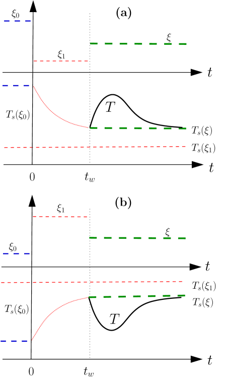
Figure 1: Sketch of the drive time dependence for the cooling and heated protocols. The resulting normal temperature evolution is depicted. The system is first in a non-equilibrium steady state at temperature $T_{s}(\xi_{0}$) under a drive $\xi_{0}$. $T(t_{w})$ coincides with $T_{s}(\xi)$. (a) Cooling protocol: The driving $\xi_{1}$ in the waiting time window $0<t<t_{w}$ is smaller than its initial value $\xi_{0}$, and the granular temperature would display a maximum before returning to its steady value for $t>t_{w}$. (b) Heating protocol: We have that $\xi_{1}>\xi_{0}$ and the granular temperature would display a minimum for $t>t_{w}$.

We are interested in analyzing the following experiment. First, we let a system of inelastic hard particles reach the steady state corresponding to some value of the driving, say $\xi_{0}$. Then, at $t=0$ we quench the driving to either $\xi_{1}<\xi_{0}$ (cooling protocol), or to $\xi_{1}>\xi_{0}$ (heating protocol), and the system subsequently evolves for a time $t_{w}$, the waiting time. At $t=t_{w}$, we measure the granular temperature and suddenly change the driving to the value $\xi$ such that the stationary granular temperature $T_{\text{s}}(\xi)$ equals the measured value at $t_{w}$, $T(t=t_{w})$. This amounts to $\xi_{1}<\xi<\xi_{0}$ in the cooling case, and $\xi_{1}>\xi>\xi_{0}$ in the heated one, see Fig. 1. If the state of the system were completely determined by the granular temperature, as is the case in the homogeneous cooling state, the temperature would remain constant for $t>t_{w}$. But, since the values of the excess kurtosis for $t=t_{w}$ and for the steady state corresponding to the final driving $\xi$ are different, the granular temperature will separate from its steady value at first, pass through an extremum, and only return to its steady (initial) value for longer times. We may refer to this behavior as the Kovacs hump, because it is similar to the so-called behavior in polymers, structural glasses and other complex systems Ko63 ; Ko79 ; Br78 ; ByB02 ; MyS04 ; AAyN08 ; PyB10 ; ByL10 ; DyH11 ; RyP14 .

In the analogous experimental situation for molecular systems, when the “driving” is first lowered ($\xi_{0}\to\xi_{1}$) and afterwards increased to an intermediate value ($\xi_{1}\to\xi<\xi_{0}$), the measured quantity, typically the volume Ko63 ; Ko79 ; MyS04 ; ByL10 or the energy Br78 ; ByB02 ; AAyN08 ; PyB10 ; DyH11 ; RyP14 , always passes through a maximum. An analogous behavior is expected for any physical quantity that increases with increasing temperature. On the other hand, within the heated protocol, a minimum is expected, as theoretically predicted by linear response theory PyB10 . Moreover, in the nonlinear regime, the existence of this minimum for the heated protocol has been recently checked for a simple model DyH11 . We will refer to this behavior, in which the time derivative of the energy changes sign at $t_{w}$, that is, the energy displays a rebound, as ‘normal’. It must be stressed here that the final state of the granular gas is not an equilibrium one, but an out-of-equilibrium stationary state, and thus the behavior of the granular temperature may be different.

III.1 Analytical results

The evolutions in the waiting window ($0\leq t\leq t_{w}$), and for $t\geq t_{w}$ both obey the differential equations (23), but with different initial conditions. At $t=0$, we have $A_{2}=1$ with either $\beta<1$ (cooling protocol) or $\beta>1$ (heating protocol). At $t=t_{w}$, a ’reversed’ condition should be enforced, with $\beta=1$ while $A_{2}$ results from the dynamics in the waiting window. $A_{2}(t_{w})$ turns out to be larger than 1 for the cooling protocol, and smaller than 1 in the heated case (see Sec. IV.2). Since the waiting time dynamics only enters through the value of $A_{2}(t_{w})$, we assume the latter given, and concentrate on the evolution at $t>t_{w}$. We shall use the rescaled time $\uptau$ introduced in (24), with $\uptau_{w}=\zeta_{0}\sqrt{T_{\text{s}}}\,t_{w}/2$.

Figure 2: Plot of $a_{2}^{\text{HCS}}/a_{2}^{\text{s}}$ as a function of the restitution coefficient $\alpha$, for a system of inelastic hard disks ($d=2$), following from the accurate expressions obtained in SyM09 . The top and bottom insets show the excess kurtosis for the steady state $a_{2}^{\text{s}}$ and the parameter $B$ as functions of $\alpha$, as given by Eq. (12) and (17), respectively.

Equations (23) with the initial conditions

$$\beta(\uptau=\uptau_{w})=1,\quad A_{2}(\uptau=\uptau_{w})\equiv A_{2}^{\text{ini}},$$ (25)

do not seem to admit an analytical solution, but an approximate and accurate method can be found in the following way. The initial value of $A_{2}$ is of the order of unity: In the cooling case, $A_{2}$ is bounded from above by $a_{2}^{\text{HCS}}/a_{2}^{\text{s}}$, shown in Fig. 2 and, in the heated case, we have that $0<A_{2}^{\text{ini}}<1$, as shown in Sec. IV.2 below. The idea is next to expand both $\beta$ and $A_{2}$ in powers of $a_{2}^{\text{s}}$. The rationale for this expansion is the smallness of $a_{2}^{\text{s}}$ throughout the whole inelasticity range, namely $|a_{2}^{\text{s}}|\leq 0.086$. Thus we introduce the series expansions

$$\beta(\uptau)=\beta_{0}(\uptau)+a_{2}^{\text{s}}\beta_{1}(\uptau)+\ldots,$$ (26a)

$$A_{2}(\uptau)=A_{20}(\uptau)+a_{2}^{\text{s}}A_{21}(\uptau)+\ldots,$$ (26b)

into (23), and write the subsequent equations up to linear order in $a_{2}^{\text{s}}$. To the zero-th order we have

$$\frac{d\beta_{0}}{d\uptau}=1-\beta_{0}^{3},\quad\beta_{0}\frac{dA_{20}}{d\uptau}=4\left[(1-\beta_{0}^{3})A_{20}+B(1-A_{20})\right],$$ (27)

submitted to the initial conditions $\beta_{0}(\uptau=\uptau_{w})=1$ and $A_{20}(\uptau=\uptau_{w})=A_{2}^{\text{ini}}$. Therefore, $\beta_{0}(\uptau)=1$, $\forall\uptau$,

$$\quad\frac{dA_{20}}{d\uptau}=-4B\left(A_{20}-1\right).$$ (28)

The zero-th order solution is then

$$\beta_{0}(\uptau)=1,$$ (29a)

$$\quad A_{20}(\uptau)=1+\Delta A_{2}^{\text{ini}}e^{-4B(\uptau-\uptau_{w})},\quad\Delta A_{2}^{\text{ini}}\equiv A_{2}^{\text{ini}}-1.$$ (29b)

To this order, the granular temperature $\beta_{0}$ remains constant while $A_{20}$ relaxes exponentially from its initial to its steady state value with a characteristic time (in the $\uptau$ scale)

$$\uptau_{c}=(4B)^{-1}.$$ (30)

There is consequently no memory effect to zeroth order.

The equation for the first order contribution to the scaled temperature is

$$\frac{d\beta_{1}}{d\uptau}=-3\beta_{1}+\frac{3}{16}\Delta A_{2}^{\text{ini}}e^{-4B(\uptau-\uptau_{w})},\quad\beta_{1}(\uptau=\uptau_{w})=0,$$ (31)

whose solution is readily obtained as

$$\beta_{1}(\uptau)=\gamma\Delta A_{2}^{\text{ini}}\left(e^{-3(\uptau-\uptau_{w})}-e^{-4B(\uptau-\uptau_{w})}\right).$$ (32)

We have introduced the definition

$$\gamma=\frac{3}{16(4B-3)}>0,$$ (33)

which is positive definite because $B>3/4$, see Fig. 2. The parameter $\gamma$ depends on the restitution coefficient $\alpha$ and the dimension of space $d$, as does $B$. Note that we have only needed the zero-th order approximation $A_{20}$ for calculating the evolution of the temperature up to first-order in the perturbation parameter $a_{2}^{\text{s}}$, that is, $\beta_{1}$. This stems from the mathematical structure of the equation for $\beta$ in (23), in which $A_{2}$ only appears in the term proportional to $a_{2}^{\text{s}}$. We will consider the first-order correction $A_{21}$ to the excess kurtosis in Sec. V, in connection with the long time behavior of the solution.

Equation (32) implies that the sign of $\beta_{1}(\uptau)$ is the same as the sign of $A_{2}^{\text{ini}}-1$, which can be shown to be positive for the cooling procedure, and negative in the heated case. We will come back to this feature in Sec. IV.2. The time evolution for the temperature, obtained by substituting (29a) and (32) into (26a), is given by

$$\beta(\uptau)-1 = a_{2}^{\text{s}}\gamma\Delta A_{2}^{\text{ini}}\left(e^{-3(\uptau-\uptau_{w})}-e^{-4B(\uptau-\uptau_{w})}\right)$$

$$= \gamma\left(a_{2}^{\text{ini}}-a_{2}^{\text{s}}\right)\left(e^{-3(\uptau-\uptau_{w})}-e^{-4B(\uptau-\uptau_{w})}\right),$$

up to higher order terms in $\mathcal{O}(a_{2}^{\text{s}})^{2}$. Thus, the sign of the “distance” $\beta-1$ of the granular temperature to its steady value is the same as that of $(a_{2}^{\text{ini}}-a_{2}^{\text{s}})$. If $\alpha$ is changed, it affects both $a_{2}^{\text{s}}$ and $a_{2}^{\text{ini}}$ so that $(a_{2}^{\text{ini}}-a_{2}^{\text{s}})$ and $a_{2}^{\text{s}}$ share the same sign, which changes at a certain value of the restitution coefficient, $\alpha_{c}\simeq 1/\sqrt{2}\simeq 0.707$ rque88 : as a consequence, $a_{2}^{\text{s}}>0$ for $\alpha<\alpha_{c}$ while $a_{2}^{\text{s}}<0$ for $\alpha>\alpha_{c}$, see the top inset in Fig. 2. We now restrict the discussion to cooling protocols. The above reasoning implies that for high inelasticities, namely $\alpha<\alpha_{c}$, $\beta-1>0$ and then $\beta$ has a maximum while the granular temperature has a minimum (remember that $T=T_{\text{s}}/\beta^{2}$). The situation reverses for small inelasticities, $\alpha>\alpha_{c}$, for which $\beta-1<0$. Then, $\beta$ has a minimum, which corresponds to a maximum of the granular temperature. On the other hand, for heating protocols, the phenomenology is reversed, but ruled by very similar mechanisms. For $\alpha>\alpha_{c}$, $T$ shows a minimum, whereas for $\alpha<\alpha_{c}$, it exhibits a maximum. A more physical explanation will be provided in subsection IV.1.

It should be noted here that from the structure of Eq. (LABEL:2.13), the shape of the hump (the $\uptau$ dependence) and its amplitude are factorized. In other words, Eq. (LABEL:2.13) can be rewritten as

$$\beta(\uptau)-1 = g(\uptau_{w})\,h(\uptau-\uptau_{w}),$$ (35a)

$$g(\uptau_{w}) = a_{2}^{\text{s}}\Delta A_{2}^{\text{ini}}=a_{2}^{\text{ini}}-a_{2}^{\text{s}},$$ (35b)

$$h(s) = \gamma\left(e^{-3s}-e^{-4Bs}\right)>0.$$ (35c)

The prefactor $g(\uptau_{w})$ contains all the information about the details of the protocol in the waiting time window, that is, the dependence of the hump not only on $t_{w}$ but also on $\{\xi_{0},\xi_{1}\}$, while $h(\uptau-\uptau_{w})$ determines its shape. We shall show in Sec. IV.2 that $\Delta A_{2}^{\text{ini}}$ has a definite sign for both cooling and heating protocols, so that $g$ also determines the sign of the hump through the steady value of the excess kurtosis $a_{2}^{\text{s}}$ or, equivalently, $a_{2}^{\text{ini}}-a_{2}^{\text{s}}$.

Equation (LABEL:2.13) or (35) gives then the lowest order expression for the Kovacs hump, within the theoretical framework we have just developed. It clearly shows that the granular temperature is not enough for describing the state of uniformly heated granular gases, as has been already claimed by other means GMyT12 ; GMyT13 . If that were the case, no hump at all would be present when the system is prepared with the correct initial granular temperature for the subsequent driving, within our à la Kovacs program. On the other hand, the existence of the Kovacs hump does not directly follow from the non-Maxwellian character of the velocity distribution. Indeed, although the velocity distribution of a granular gas is generically non-Gaussian, the granular temperature may completely specify its state in some situations. This is the case for the homogeneous cooling state but also for the equivalent system driven by the so-called Gaussian thermostat. Therein, particles are accelerated between collisions by a force proportional to their own velocity MyS00 ; Lu01 ; BRyM04 , and no Kovacs hump would be observed if an analogous stepwise driving procedure were followed.

III.2 Numerical results

We compare here the analytical expression for the Kovacs hump to the results obtained by direct Monte Carlo simulations Bi94 of the Boltzmann-Fokker-Planck equation. We have used a system of $N=10^{4}$ hard disks ($d=2$) of unit mass, $m=1$, and unit diameter, $\sigma=1$, with the collision rule (1). The results have been averaged over a large number (ranging from $N_{T}=10^{5}$ to $1.5\times 10^{6}$) of realizations of the stochastic dynamics of the system. The stochastic thermostat is taken into account by the procedure first introduced in Ref. ENTyP99 . Over each trajectory, the hard disks are submitted to random kicks every $N_{c}=N/10^{3}=10$ collisions. In the kick, each component of the velocity of every particle is incremented by a random number extracted from a gaussian distribution of variance $\xi^{2}\Delta t$, where $\Delta t$ is the time interval corresponding to the number of collisions $N_{c}$. Moreover, every $N/10^{2}=100$ collisions, a possible non-vanishing center of mass velocity is eliminated to enforce conservation of momentum and avoid a spurious drift of the center-of-mass velocity.

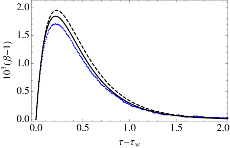
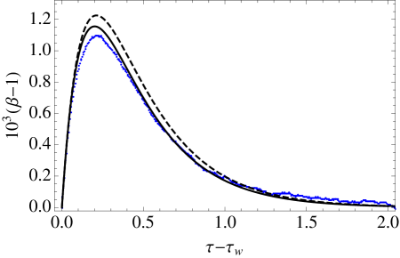
Figure 3: Plot of the Kovacs hump for $\alpha=0$ (top) and $\alpha=0.3$ (bottom). The simulation curves (points) have been averaged over $10^{5}$ trajectories, and they are compared to (i) the raw theoretical curve (LABEL:2.13), evaluated with the theoretical expressions for the parameters $a_{2}^{\text{s}}$, $B$, and $a_{2}^{\text{HCS}}$ (dashed line) and (ii) the improved theory obtained by inserting into (LABEL:2.13) the value of the $B$-parameter given by the Monte Carlo simulation (solid line). The second route improves the agreement between theory and simulation. The specific values of the parameters for each of the plotted curves are given in Table 1. Note the smallness of $\beta-1$, which is of the order of $10^{-3}$ in both cases.

	$\alpha=0$	$\alpha=0.3$	$\alpha=0.8$
$B$ from DSMC	1.802	1.920	2.440
$B$ from (17)	1.422	1.555	2.602
$B$ from (21)	1.652	1.753	2.507

Table 1: Values of the excess kurtosis decay rate $B$, corresponding to the plots in Figs. 3 and 5. For comparison with Monte Carlo data, Eq. (21) has been used.

Our analytical predictions reveal that the Kovacs effect is all the more pronounced as the difference $|a_{2}^{\text{ini}}-a_{2}^{\text{s}}|$ is large. Quite intuitively, there are two ways to maximize $|a_{2}^{\text{ini}}-a_{2}^{\text{s}}|$: either taking $\xi_{1}\ll\xi_{0}$ (equivalently $T_{s}(\xi_{1})\ll T_{s}(\xi_{0})$ in the cooling case, or in the heated situation, reversing all inequalities. We concentrate here on the cooling protocol, for which we have performed simulations such that the choice $\xi_{1}\ll\xi_{0}$ guaranties that the system, in the waiting time window, has an excess kurtosis that quickly evolves towards its free cooling counterpart; thus, $A_{2}(\uptau_{w})=a_{2}^{\text{HCS}}/a_{2}^{\text{s}}$. We will discuss in subsection IV.2 the cases of finite $\xi_{1}/\xi_{0}$. For the sake of simplicity, we have always used $\xi_{1}=0$, which allows us to simplify the simulation procedure, see below.

Let us explain how we calculate in the simulations the final value of the driving $\xi$ from the value of the granular temperature $T(t_{w})$ at the end of the waiting time window. For an arbitrary value of the intermediate driving $\xi_{1}$: (i) run all the realizations until the waiting time, (ii) obtain the granular temperature $T(t_{w})$ averaging over all the realizations, (iii) determine the final value of the driving $\xi$ therefrom, and (iv) continue running all the realizations. This numerical procedure introduces some (in general unavoidable) numerical errors, stemming from the fluctuations of the granular temperature over the different realizations. Nevertheless, we may take advantage of the value of the driving in the waiting time window, $\xi_{1}=0$, to eliminate these fluctuations and minimize the numerical error. For long enough waiting times long_enough_tw , the system cools in the homogenous cooling state, a regime where all the time evolution may be encoded in the granular temperature. Then, we proceed in the following way: (i) We choose a value of the final driving $\xi$, and calculate the corresponding steady granular temperature $T_{\text{s}}(\xi)$, (ii) run each realization until the shortest time $t$ such that $T(t)<T_{\text{s}}(\xi)$, (iii) rescale all the velocities of the particles with a factor $\sqrt{T_{\text{s}}(\xi)/T(t)}$, so that $T(t)=T_{\text{s}}(\xi)$, thus effectively eliminating the granular temperature fluctuations at the waiting time, and (iv) continue running all the realizations.

In Fig. 3, we show the comparison between the numerical computation of the Kovacs hump and our theoretical prediction, in the high inelasticity regime $\alpha<\alpha_{c}\simeq 0.707$. Namely, we have considered (a) $\alpha=0$ and (b) $\alpha=0.3$. In both cases, there are two theoretical curves: the dashed line corresponds to the raw evaluation of Eq. (LABEL:2.13) with the theoretical values of $a_{2}^{\text{s}}$, $a_{2}^{\text{HCS}}$ and $B$ given by Eqs. (12), (18) and (21), respectively. Although the qualitative agreement is reasonable, there are quantitative discrepancies. This is not surprising. While the analytical predictions for $a_{2}^{\text{s}}$ and $a_{2}^{\text{HCS}}$ turn out reliable for our purposes, Eq. (21) does not fare as well, and may be plagued by nonlinear effects, as is the case for Eq. (17) GMyT12 . Therefore, we have followed an alternative route: We first measure $B$ from the relaxation of the excess kurtosis, as embodied in relation (29b), see Fig. 4, which clearly exhibits an exponential behavior. The corresponding value of $B$ is then inserted in Eq. (LABEL:2.13), to give the solid line in Fig. 3. A posteriori, we have also compared the values of $B$ to their analytical counterparts, as seen in Table 1. The inaccuracy of the theoretical estimate is of approximately $10\%$ for Eq. (21), and 20% with Eq. (17), consistently with the situation found in previous studies GMyT12 . It appears that once an accurate value of the relaxation parameter $B$ is known, quantitative predictions can be made.

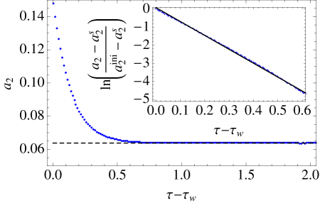
Figure 4: Decay of the excess kurtosis from its initial to its steady state value. Plotted is the simulation curve obtained by DSMC (points) for $\alpha=0.3$. The long time limit is very close to its predicted value $a_{2}^{\text{s}}=0.00638$, following from Eq. (12) and shown by the dashed line. In the inset, the same decay but on a logarithmic scale (points). From the linear slope, we directly measure the parameter $B$, to be inserted into the theoretical expression for the Kovacs hump, Eq. (LABEL:2.13). The obtained values are given in Table 1.

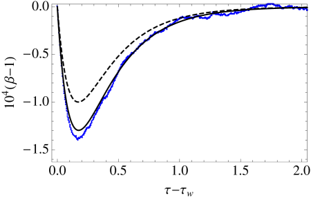
Figure 5: Plot of the Kovacs hump for $\alpha=0.8$. The meaning of the different symbols and lines is the same as in Fig. 3. Note that the sign of $\beta-1$ is reversed, $\beta-1<0$ as the restitution coefficient $\alpha>\alpha_{c}\simeq 0.707$.

Figure 5 shows the Kovacs hump for a smaller value of the inelasticity, namely $\alpha=0.8>\alpha_{c}$. As predicted by the theory, the sign of $\beta-1$ is reversed, since $a_{2}^{\text{s}}<0$ for $\alpha>\alpha_{c}$. The simulation curve has been averaged over $1.5\times 10^{6}$ trajectories, because in this region not only $|a_{2}^{\text{s}}|$ but also $\Delta A_{2}^{\text{ini}}$ are of smaller magnitude, see Fig. 2. Thus, the amplitude of the hump is reduced roughly tenfold as compared to those in Fig. 3. For $\alpha=0.8$, the error in the theoretical estimate of $(a_{2}^{\text{HCS}}-a_{2}^{\text{s}})$ is of the order of $20$ per cent, roughly an order of magnitude larger than the one for the highly dissipative cases of Fig. 3. Therefore, in order to obtain a good agreement between theory and simulation (solid line), we have to insert into (LABEL:2.13) both the measured value of $B$ and the simulation value of the excess kurtosis difference $(a_{2}^{\text{HCS}}-a_{2}^{\text{s}})$ difference . A similar situation, in which not only $B$ but also the excess kurtosis had to be taken from the simulations, was found in the analysis of the universal reference state of Ref. GMyT12 in the same range of inelasticities.

IV Sign and magnitude of the extremum

IV.1 Physical origin of the effect

We attempt here a more physical explanation of the mechanism at work here, which is, expectedly, very different from that in glassy systems. In essence, the effects we observe are subtle consequences of energy dissipation, Without loss of generality, we focus on the cooling protocol. An important feature is the shape of the velocity distribution $f({\bm{v}},t)$, through the sign of the excess kurtosis $a_{2}$. Is it “flatter” than the Gaussian (so-called platykurtic, with $a_{2}<0$), or is it “thinner” (so-called leptokurtic, with $a_{2}>0$) ? Distributions with $a_{2}<0$ dissipate less energy (and conversely, more energy when $a_{2}>0$). Indeed, one can show that to linear order in the excess kurtosis,

$$\frac{\langle v_{12}^{n}\rangle}{\langle v_{12}^{n}\rangle_{0}}\,=\,1\,+\,a_{2}\frac{n(n-2)}{16},$$ (36)

where the average with index 0 refers to a Gaussian distribution of the same variance, and $v_{12}$ is the modulus of the relative velocity. The correction to unity vanishes when $n=0$ (normalization) and $n=2$ (equality of variances). Energy dissipation is related to the moment $n=3$ (one $v$ coming from the collision frequency, and a $v^{2}$ from the fact that we are interested in the kinetic energy). Thus $\langle v_{12}^{3}\rangle<\langle v_{12}^{3}\rangle_{0}$, for $a_{2}<0$ rque50 .

We start by discussing the behavior of the system in the cooling protocol, see Fig. 1 (a), in which the driving in the waiting time window is smaller than the initial one, $\xi_{1}<\xi_{0}.$ Moreover, and for the sake of simplicity, we focus in the limiting case $\xi_{1}=0$, in which the system freely cools for $0<t<t_{w}$. We analyze the case $\xi_{1}\neq 0$ in Sec. IV.2, in which we show that this change only affect the magnitude of the effect, but not its sign. Close to elasticity, $a_{2}<0$, for both driven and undriven gases (platykurtic behavior). It is quite difficult to shape an intuition for the sign. It may be tempting to argue that it is a means for the system to minimize energy dissipation, in spite of the lack of a general principle holding for such non-equilibrium systems. What is more intuitive is that the unforced system shows stronger non Gaussianities than the driven one, which benefits from stochastic kicks from the forcing, $|a_{2}^{\text{HCS}}|/|a_{2}^{\text{s}}|>1$ . Hence, at $t=t_{w}$, the system is in a state where $a_{2}$ is more negative than it asymptotically will be, and therefore, energy dissipation is, transiently, less. This implies that $T$ shows a maximum (or $\beta$ a minimum, as we observe).

The above scenario applies as long as dissipation is not too large ($\alpha>\alpha_{c}=1/\sqrt{2}$). On the other hand, for $\alpha<\alpha_{c}=1/\sqrt{2}$, the driven and undriven systems become leptokurtic ($a_{2}>0$, in order, in a hand-waving fashion, to cope with large dissipation). We can subsequently follow the same reasoning as above, which explains the anomalous effect. The undriven kurtosis is larger than the driven one (the driven $f$ is always the most Gaussian), so that the larger value of $a_{2}$ at $t_{w}$ brings extra dissipation. Thus, $T$ shows an undershooting (maximum of $\beta$).

For heating protocols, see Fig. 1(b), we next focus on the limiting case $\xi_{1}\to\infty$. Again, a finite value of the driving in the waiting time window $\xi_{1}$ does not change the sign of the effect but only its magnitude, see next section. For a very large value of $\xi_{1}$, the system rapidly evolves to a gaussian distribution with $a_{2}=0$ in the waiting time window. Therefore, we always have that $|a_{2}^{\text{s}}|>|a_{2}^{\text{ini}}|=0$ and following the same line of reasoning as in the cooling case, it is easily shown that the separation of the temperature from its steady value is simply reversed.

The above picture remains valid for a closely related thermostat, in which the energy injection is the same but the bath provides an additional friction force CVyG13 . In particular, the value of the excess kurtosis for that thermostat also verifies that $|a_{2}^{\text{s}}|<|a_{2}^{\text{HCS}}|$. The introduction of this additional friction force allows the system to reach a well-defined steady state even in the elastic limit $\alpha=1$, in which the dissipation stemming from collisions disappears.

IV.2 The optimal waiting time

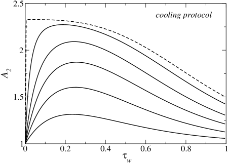
Figure 6: Evolution of excess kurtosis ratio, $A_{2}(\uptau_{w})\equiv a_{2}(\uptau_{w})/a_{2}^{\text{s}}$, as a function of waiting time, within the cooling protocol at $\alpha=0.3$. From bottom to top, the curves correspond to $T_{s}(\xi_{0})/T_{s}(\xi_{1})=2,4,9,25$ and 200. The upper dashed curve is for the limit $T_{s}(\xi_{1})/T_{s}(\xi_{0})\to 0$. Note that $A_{2}(\uptau_{w})$ defines the quantity $A_{2}^{\text{ini}}$ used throughout. For a given value of $\alpha$, the maximum possible $A_{2}$ is $a_{2}^{\text{HCS}}/a_{2}^{s}$. For $\alpha=0.3$, Fig. 2 indicates that this ratio is close to $2.33$, which is consistent with the maximum of the dashed curve.

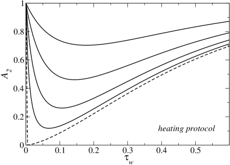
Figure 7: Same as Fig. 6 but for the heated protocol. Here, from top to bottom: $T_{s}(\xi_{1})/T_{s}(\xi_{0})=2,4,9,25$. The lower dashed curve is for $T_{s}(\xi_{1})/T_{s}(\xi_{0})\to\infty$

We now return to the cooling protocol, in the limiting case where $\xi_{1}/\xi_{0}$ is close to zero. At $\xi_{1}/\xi_{0}=0$, the waiting time $t_{w}$ can be arbitrarily large, since $a_{2}$ will evolve to $a_{2}^{\text{HCS}}$, and the longer one waits (in real time scale, not in the $\tau$ scale, see below), the stronger the effect. In general however, there is an optimal value of $t_{w}$, which depends on the ratio $T_{s}(\xi_{1})/T_{s}(\xi_{0})$, for which the amplitude of the Kovacs response is maximal. The reason is that the difference in kurtosis, $|a_{2}(t_{w})-a_{2}^{\text{s}}|$, should be maximized. If one spends too much time in the waiting window, the system can attain its non-equilibrium steady state, $a_{2}(t_{w})$ then reaches the value $a_{2}^{\text{s}}$ ($A_{2}\to 1$), and the humps disappears. This holds for both the cooling ($\xi_{1}<\xi_{0}$) and the heated ($\xi_{1}>\xi_{0}$) protocols, see Figures 6, 7 and 8. These figures therefore exhibit an extremum at a particular value of $\uptau_{w}$, which provides the optimal waiting time. It can be observed that in the $\uptau$ scale, this optimum depends only weakly on $\xi_{1}/\xi_{0}$ (or equivalently on $T_{s}(\xi_{1})/T_{s}(\xi_{0})$), and likewise, quite weakly on dissipation.

The trends observed in the Figures, with a maximum (resp. minimum) in the cooling (resp. heating) case, can be understood as in Sec. IV.1, and are fully consistent with the argument put forward there. In the extreme case $T_{s}(\xi_{1})/T_{s}(\xi_{0})\to\infty$ (that is, $\xi_{1}/\xi_{0}\to\infty$), the velocity distribution is provided enough time to become Gaussian, with thus a vanishing $a_{2}$ (and $A_{2}$). This is the behavior shown in Fig. 7. Yet, the dashed line also shows that for any finite $T_{s}(\xi_{1})/T_{s}(\xi_{0})$, no matter how large, the optimal waiting time becomes vanishingly small in the $\tau$ scale, which reflects the fact that under extreme forcing $\xi_{1}$, the system is so much driven that it is able to quickly reach its steady-state. It is at this point interesting to turn to the dashed line in Fig. 6 for the cooled extreme case $\xi_{1}/\xi_{0}\to 0$. It also reveals that the optimal $\tau_{w}$ also vanishes, whereas, on intuitive grounds, it should be that one can wait arbitrarily long without seeing the system depart from the homogeneous cooling state it quickly attains. In other words, one may expect that the optimal waiting time should diverge upon decreasing the forcing. This is the case, but it can only be appreciated by returning to the original $t$ scale: it turns out that the optimal $t_{w}\propto\tau_{w}/\sqrt{T_{s}(\xi_{1})}$ diverges when $\xi_{1}\to 0$, due to the vanishing of $T_{s}(\xi_{1})$.

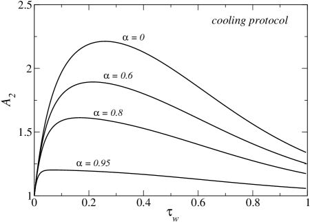
Figure 8: Excess kurtosis ratio as a function of waiting time (cooling protocol), for different dissipations, and $T_{s}(\xi_{1})/T_{s}(\xi_{0})=1/25$.

We attempt here a summary of the main results reported in this Section. The Kovacs-like protocol used throughout this paper can be described by three dimensionless parameters: (i) the restitution coefficient $\alpha$, (ii) the ratio $\xi_{1}/\xi_{0}$ of the intermediate driving $\xi_{1}$ to the initial one $\xi_{0}$, and (iii) the dimensionless waiting time $\uptau_{w}$, which in turn fixes the ratio $\xi/\xi_{1}$. The sign of the hump is completely determined by the first two, $\alpha$ and $\xi_{1}/\xi_{0}$, while the third only affects the magnitude of the extremum. A phase diagram of the Kovacs hump is sketched in Fig. 9. The “normal” behavior is similar to the one observed in molecular systems when controlling the bath temperature and measuring the energy (or the volume). The lines in the diagram indicate the values of the parameters for which no Kovacs hump would be observed. The solid line $\xi_{1}=\xi_{0}$ separating heating and cooling protocols delineates a “trivial” boundary, with no change in the driving and thus no hump. On the other hand, the dashed line $\alpha=\alpha_{c}$ separating the low and high inelasticity regions is less expected, and follows from the accurate prediction of the first Sonine approximation for the change of sign in the Kovacs hump.

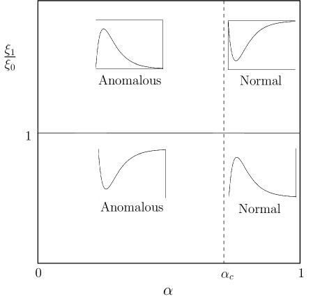
Figure 9: Phase diagram of the Kovacs hump. The line $\xi_{1}/\xi_{0}=1$ (solid) separates the “cooling” ($\xi_{1}<\xi_{0}$) and the “heating” ($\xi_{1}>\xi_{0}$) protocols. The dashed line $\alpha=\alpha_{c}=1/\sqrt{2}$ separates systems with “high inelasticity” ($\alpha<\alpha_{c}$) from those with “low inelasticity” ($\alpha>\alpha_{c}$). Note that the plots are for the granular temperature $T$, a maximum in $T$ corresponds to a minimum in the $\beta$ variable defined in Eq. (14).

V Long time behavior and compatibility with the universal reference state

On close inspection, the trends reported above for the time evolution of $\beta$ are not compatible with the requirement that the system should asymptotically evolve towards the universal state brought to the fore in Ref. GMyT12 . We discuss and resolve that question here. In a nutshell, the time evolution is slightly more complex than the simplified expressions obtained in Section III.1. For the sake of simplicity, we use in this section the shifted time variable $\uptau=\zeta_{0}\sqrt{T_{s}}(t-t_{w})/2$, which vanishes at $t=t_{w}$. Let us consider the equation for the first-order correction to the excess kurtosis,

$$\frac{dA_{21}}{d\uptau}+4BA_{21}=-\left[(12-4B)A_{20}+4B\right]\beta_{1}.$$ (37)

We do not write here its complete solution, but only its leading behavior for long times. The solution of (37) is a linear combination of exponentials with different relaxation times. For $\uptau\to\infty$, the rhs of (37) behaves, to dominant order, as

$$h(\uptau)=-12\gamma\Delta A_{2}^{\text{ini}}e^{-3\uptau},$$ (38)

as follows from Eq. (29b) and (32). The term in $A_{21}$ coming therefrom is

$$A_{21}^{h}(\uptau)=-64\gamma^{2}\Delta A_{2}^{\text{ini}}e^{-3\uptau},$$ (39)

and asymptotically dominates

$$A_{21}(\uptau)\sim A_{21}^{h}(\uptau),\quad\uptau\gg 1.$$ (40)

Interestingly, this term is much bigger than $A_{20}(\uptau)$ for very long times, and thus gives the long time tendency to the steady value of the rescaled excess kurtosis,

$$A_{2}(\uptau)-1\sim a_{2}^{\text{s}}A_{21}^{h}(\uptau),\quad\uptau\gg 1.$$ (41)

The condition for the asymptotic result in (41) to hold is, more concretely, $\exp(-4B\uptau)\ll\exp(-3\uptau)$ or, equivalently, $\exp[-(4B-3)\uptau]\ll 1$. It is worth noting that the sign of $A_{21}^{h}(\uptau)$ is opposite to that of $\Delta A_{2}^{\text{ini}}$ and therefore different from that of the zero-th order contribution $A_{20}(\uptau)-1$, see Eq. (29b). As $a_{2}^{\text{s}}<0$ for weakly dissipative systems, $\alpha>\alpha_{c}$ while $a_{2}^{\text{s}}>0$ in the highly dissipative case, $\alpha<\alpha_{c}$, Eq. (41) predicts that, for long times $\uptau\gg 1$, the sign of $A_{2}-1$ is the opposite to that of $A_{20}-1$ for $\alpha<\alpha_{c}$. This means that $A_{2}$ has a minimum and tends to unity from below in the highly dissipative case. This behavior was overlooked by the analysis performed in previous sections. The effect is quite small and thus difficult to measure in the simulations, but it has important theoretical consequences. In Ref. GMyT12 it was proved that, for long enough times, a uniformly heated granular gas reaches the universal reference $\beta$-state, over which all the time dependence can be encoded in $\beta$. In other words, for long enough times, all the moments of the velocity distribution function (for instance, the excess kurtosis) forget their initial conditions and become only a function of the “distance” $\beta$ to the steady state. Afterwards, for even longer times, $\beta$ approaches its steady value. For the excess kurtosis, and in the linear regime close to the steady state, this universal behavior is given by

$$A_{2}-1\sim\left.\frac{dA_{2}}{d\beta}\right|_{\beta=1}(\beta-1)=-\frac{12}{4B-3}(\beta-1).$$ (42)

The value of the derivative $dA_{2}/d\beta|_{\beta}=1$ has been calculated by applying L’Hôpital rule to Eq. (19) of Ref. GMyT12 .

If we take the lowest order approximation for both $A_{2}-1$, which is $A_{20}-1$, and for $\beta-1$, which is given by $\beta_{1}$, we have that

$$\lim_{\uptau\to\infty}\frac{A_{20}-1}{\beta-1}=0,$$ (43)

in strong disagreement with (42), which predicts a value $-12/(4B-3)<0$ instead. This problem is mended if we consider, as should be done, $A_{2}-1$ and $\beta-1$ up to the same order. Since the dominant term for long times in the decay of $A_{2}$ is proportional to $A_{21}^{h}$, as given by (41), and the long time behavior of $\beta-1$ can be straightforwardly inferred from (LABEL:2.13),

$$\beta(\uptau)-1\sim a_{2}^{\text{s}}\gamma\Delta A_{2}^{\text{ini}}e^{-3\uptau},$$ (44)

one obtains that

$$\frac{A_{2}-1}{\beta-1}\sim-64\gamma\,=\,\frac{-12}{4B-3},\quad\uptau\gg 1,$$ (45)

where the definition of $\gamma$, Eq. (33), has been used. The result in (45) is in agreement with (42).

Figure 10 shows the tendency of the system to approach the universal reference state for very long times. Although to the zero-th order the overall relaxation of the excess kurtosis to the steady state is very well described by a single exponential, see Fig. 4, for very long times $a_{2}-a_{2}^{\text{s}}$ changes sign and tends to zero from below. This is in full agreement with the approach to the universal reference state, as described by Eq. (42) or (45). The minimum is tiny, being four orders of magnitude smaller than the initial distance to the steady state for the plotted case ($\alpha=0.3$). This makes it very difficult to measure this effect in simulations. However, it is crucial from a theoretical point of view, since it shows that the theoretical approach developed here is compatible with the general long time behavior derived in Ref. GMyT12 .

Figure 10: Tendency to the universal reference state for very long times. We show a zoom of the long time behavior ($\uptau-\uptau_{w}\geq 1$) of the decay of the excess kurtosis to its steady value, $|a_{2}-a_{2}^{\text{s}}|\leq 2\times 10^{-5}$. The overall picture is that of Fig. 4, which also corresponds to $\alpha=0.3$, for which $a_{2}^{\text{ini}}-a_{2}^{\text{s}}\simeq 0.086$. Plotted here is the excess kurtosis decay obtained from (i) the numerical integration of Eq. (23) with initial conditions (25) (solid line) (ii) the asymptotic behavior given by Eq. (41) and (39) (dashed line).

VI Final remarks

In conclusion, we have studied from a granular gas perspective a memory effect that pertains to glassy phenomenology. A striking consequence of the analysis is that the sign of the Kovacs hump changes as the restitution coefficient is varied from the quasi-elastic limit $\alpha\to 1^{-}$ to the completely inelastic case $\alpha=0$. There is a critical value of the restitution coefficient $\alpha_{c}$, which coincides with the point at which the stationary value of the excess kurtosis changes sign. First, we recapitulate the behavior for cooling protocols as the one depicted in Fig. 1(a). For weakly dissipative systems, in the sense that $\alpha>\alpha_{c}$, the granular temperature passes through a maximum, larger than its corresponding steady value $T_{\text{s}}$ ($\beta=\sqrt{T_{\text{s}}/T}<1$). The sign of the hump changes for highly dissipative systems, in which $\alpha<\alpha_{c}$: the temperature passes through a minimum ($\beta>1$). Conversely, for heating protocols, in which $\xi_{0}<\xi<\xi_{1}$ as sketched in Fig. 1(b), we simply have a reversal of the sign of the hump: the granular temperature displays a minimum for small inelasticity, $\alpha>\alpha_{c}$ and a maximum for high inelasticity $\alpha<\alpha_{c}$. Table 2 summarizes the phenomenology. On the other hand, in a molecular system, the measured quantity in the analogous experimental situation molecular always exhibits a maximum (resp. minimum) in the cooling (resp. heating) protocol. This stems from the mathematical structure of the analytical expression for the Kovacs hump within linear response theory, but the same result seems to remain valid in the nonlinear regime PyB10 ; DyH11 ; RyP14 .

protocol	inelasticity	$\alpha$	$a_{2}^{\text{ini}}-a_{2}^{\text{s}}$	dissipation	$T$ hump	Kovacs effect
cooling	“low”	$\;>\alpha_{c}\;$	$\;<0\;$	smaller than stationary	maximum	normal
cooling	“high”	$\;<\alpha_{c}\;$	$\;>0\;$	larger than stationary	minimum	anomalous
heating	“low”	$\;>\alpha_{c}\;$	$\;>0\;$	larger than stationary	minimum	normal
heating	“high”	$\;<\alpha_{c}\;$	$\;<0\;$	smaller than stationary	maximum	anomalous

Table 2: Hump phenomenology and the underlying physical mechanism for the cooling and heating driving protocols in Fig. 1. The ‘critical’ value of the restitution coefficient $\alpha$ is $\alpha_{c}=1/\sqrt{2}$.

Therefore, the Kovacs effect for uniformly heated granular gases is normal for small inelasticities while it is anomalous in the highly inelastic case, independently of the details of the protocol followed in the waiting time window. The intermediate value of the driving $\xi_{1}$ and the waiting time $t_{w}$ do affect the amplitude of the memory effect, but not its sign and shape, as expressed by Eq. (35) and discussed in Sec. IV. Nevertheless, there are optimal values of $\xi_{1}$ and $t_{w}$ that maximize the amplitude of the hump for a given value of the restitution coefficient. Quite intuitively, for the usual cooling protocol the optimal choice of parameters corresponds to the limit $\xi_{1}\to 0$ with a large enough $t_{w}$, such that the system ends up in the homogeneous cooling state inside the waiting time window.

In molecular systems, energy is conserved and, within the linear response regime, the shape of the Kovacs hump is closely related to the linear relaxation function of the energy from the initial temperature $T_{0}$ to the final one $T$. This direct relaxation function decays monotonically because it is proportional to the equilibrium time autocorrelation function of the energy, as stated by the fluctuation-dissipation theorem vK92 . In turn, this monotonicity assures that the Kovacs hump is always positive for the usual cooling protocol PyB10 , while it is negative for the heating protocol considered in Ref. DyH11 . Therefore, it seems worth investigating the anomalous character of the Kovacs hump found here for high dissipation. Specifically, it would be interesting to analyze the possible relation between the anomalous character of the Kovacs effect for high dissipation and the validity of the fluctuation-dissipation relation in non-equilibrium systems. In the context of granular media, there is some recent work trying to establish the validity of fluctuation-dissipation relations. PByL02 ; PByV07 ; MGyT09 ; SVGP10 ; PLyH11-12 ; BMyG12 . It seems particularly appealing to investigate simple models of dissipative systems PLyH11-12 ; BByP02 , for which the calculations may be carried out without introducing any approximations like the Sonine expansion considered here.

Our main assumptions are (i) the accurateness of the first-Sonine approximation (ii) the smallness of the excess kurtosis that makes it possible to neglect nonlinear terms in $a_{2}$. Our expression for the Kovacs hump, as given by Eq. (LABEL:2.13), is valid up to the linear order in the excess kurtosis. If nonlinear corrections in $a_{2}$ were incorporated to the time evolution equations, this linear order result would not be affected. The exponential decay of the excess kurtosis to the zero-th order, as given by $A_{20}$, is neither affected by the introduction of nonlinearities. The same is applicable to the long time behavior and the tendency to the universal reference state discussed in Sec. V. This may be surprising at first sight, because nonlinearities in $a_{2}$ should certainly change the equation for the excess kurtosis first-order correction $A_{21}$. However, these nonlinearities must vanish in the steady state (as $(A_{2}-1)^{2}$ to the quadratic order), and thus they are subdominant against the leading term as given by $h(\uptau)$, Eq. (38). The results derived throughout the paper are therefore robust.

One of the main implications of the original work by Kovacs is that it clearly showed that the experimental macroscopic variables (pressure, volume, temperature, for polymers) do not suffice to completely characterize the system state, which in general depends on the whole previous thermal history. In this sense, the existence of the Kovacs hump here, independently of its amplitude and sign (normal or anomalous), is a crisp proof that the state of the uniformly heated granular gas is not uniquely determined by its granular temperature, and other variables must be incorporated to have a complete description thereof. At first glance, this conclusion seems similar to that reached in the analysis of its universal reference $\beta$-state GMyT12 ; GMyT13 , in which it was shown that the “distance” to the steady state $\beta$ is also necessary to describe the uniformly driven granular gas. But it must be stressed that here, we go further. While the $\beta$-state reached for long times is uniquely determined by the driving $\xi$ and the granular temperature $T$, we show the relevance of explicitly keeping track of the intrinsic dynamics of non-Gaussianities, through the decoupling of $a_{2}$ and $\beta$.

In principle, a similar behavior should appear for other kinds of drivings, provided that the driving intensity and the granular temperature do not suffice to completely characterize the state of the system. Within the first Sonine approximation, the magnitude of the Kovacs hump would be proportional to the difference between the initial value of the excess kurtosis $a_{2}^{\text{ini}}$ and its steady value for the considered thermostat other_driving . In the usual cooling protocol, if a very low value of the intermediate driving $\xi_{1}$ were used, the value of the excess kurtosis after the waiting time would be close to that of the homogeneous cooling state. Therefore, non-Gaussianities are a necessary but not sufficient condition to have memory effect of the kind reported here in a driven granular gas gaussian_thermostat . In all generality, the possibility of having a transition from normal to anomalous Kovacs effect is encoded in the change of sign of $a_{2}^{\text{ini}}-a_{2}^{\text{s}}$.

The Kovacs hump in granular gases occurs over the kinetic time scale. For the time at which the temperature passes through its extremum, the system has not reached the hydrodynamic stage Re77 in which the all the time dependence of the velocity distribution function occurs through the hydrodynamic fields (density, average velocity and temperature), and initial conditions have been forgotten. Over the hydrodynamic $\beta$-state of uniformly driven gases, the decay of the temperature (or of $\beta$) to its steady value is a monotonic function of time GMyT12 ; GMyT13 . Here, this monotonicity condition is only fulfilled for times greater than that of the extremum. Then, the system reaches this hydrodynamic solution of the Boltzmann equation only for very long times, when it is linearly close to the steady state.

- (1) H. Jaeger, S. R. Nagel, and R. Behringer, Rev. Mod. Phys. 68 1259 (1996).
- (2) A. Barrat, E. Trizac, and M. H. Ernst, J. Phys.: Condens. Matter 17, S2429 (2005).
- (3) T. Pöschel and N. Brilliantov eds., Granular Gas Dynamics, (Springer, Berlin, 2003).
- (4) N. Brilliantov and T. Pöschel, Kinetic Theory of Granular Gases (Clarendon Press, Oxford, 2004).
- (5) A. Goldshtein and M. Shapiro, J. Fluid. Mech. 282, 75 (1995).
- (6) J. J. Brey, M. J. Ruiz-Montero, and D. Cubero, Phys. Rev. E 54, 3664 (1996).
- (7) T. P. C. van Noije, and M. H. Ernst, Granular Matter 1, 57 (1998).
- (8) P. K. Haff, J. Fluid. Mech. 134, 401 (1983).
- (9) D. R. M. Williams and F. C. MacKintosh, Phys. Rev. E 54, R9 (1996).
- (10) T. P. C. van Noije, M. H. Ernst, E. Trizac, and I. Pagonabarraga, Phys. Rev. E 59, 4326 (1999).
- (11) J. M. Montanero and A. Santos, Granular Matter 2, 53 (2000).
- (12) A. Santos and J. M. Montanero, Granular Matter 11, 157 (2009).
- (13) P. Maynar, M.I García de Soria, and E. Trizac, Eur. Phys. J. Special Topics 179, 123 (2009).
- (14) M. H. Ernst, E. Trizac, and A. Barrat, J. Stat. Phys. 124, 549 (2006).
- (15) K. Vollmayr-Lee, T. Aspelmeier, and A. Zippelius Phys. Rev. E 83, 011301 (2011).
- (16) M. I. García de Soria, P. Maynar, and E. Trizac, Phys. Rev. E 85, 051301 (2012).
- (17) M. I. García de Soria, P. Maynar, and E. Trizac, Phys. Rev. E 87, 022201 (2013).
- (18) A slight variant of the model can be found in P98b ; CVyG13 ; PSD13 .
- (19) C. Josserand, A. V. Tkachenko, D. M. Mueth, and H. M. Jaeger, Phys. Rev. Lett. 85, 3632 (2000).
- (20) J. J. Brey and A. Prados, Phys. Rev. E 63, 061301 (2001).
- (21) A. Barrat and V. Loreto, Europhys. Lett. 53, 297 (2001).
- (22) J. J. Brey and A. Prados, J. Phys: Cond. Matt. 14, 1489 (2002).
- (23) P. Richard, M. Nicodemi, R. Delannay, P. Ribière, and D. Bideau, Nature Materials 4, 121 (2005).
- (24) Ph. Ribière, P. Richard, P. Philippe, D. Bideau, and R. Delannay, Eur. Phys. J. E 22, 249 (2007).
- (25) A. J. Kovacs, Adv. Polym. Sci. (Fortschr. Hochpolym. Forsch.) 3, 394 (1963).
- (26) A. J. Kovacs, J. J. Aklonis, J. M. Hutchinson, and A. R. Ramos, J. Pol. Sci. 17, 1097 (1979).
- (27) S. A. Brawer, Phys. Chem. Glasses 19, 48 (1978).
- (28) L. Berthier and J. P. Bouchaud, Phys. Rev. B 66, 054404 (2002).
- (29) S. Mossa S and F. Sciortino, Phys. Rev. Lett. 92, 045504 (2004).
- (30) G. Aquino, A. Allahverdyan, and T. M. Nieuwenhuizen, Phys. Rev. Lett. 101, 015901 (2008).
- (31) A. Prados and J. J. Brey, J. Stat. Mech. P02009 (2010).
- (32) E. Bouchbinder and J. S. Langer, Soft Matter 6, 3065 (2010).
- (33) G. Diezemann and A. Heuer, Phys. Rev. E 83, 031505 (2011).
- (34) M. Ruiz-García and A. Prados, Phys. Rev. E 89, 012140 (2014).
- (35) J. Lutsko, Phys. Rev. E 63, 061211 (2001).
- (36) J. J. Brey, M. J. Ruiz-Montero, and F. Moreno, Phys. Rev. E 69, 051303 (2004).
- (37) A. Prados and E. Trizac, Phys. Rev. Lett. 112, 198001 (2014), arXiv:1404.6162.
- (38) N. V. Brilliantov and T. Pöschel, Europhys. Lett. 74, 424 (2006).
- (39) L. Landau and E. Lifshitz, Physical Kinetics (Pergamon Press, New York, 1981).
- (40) E. Trizac, Physical Review Letters 88, 160601 (2002).
- (41) J. Piasecki, E. Trizac, M. Droz Physical Review E 66, 066111 (2002).
- (42) There is a typo in the expression for of Ref. GMyT12 , concretely in the sign of the term in the denominator proportional to , which has been corrected upon writing Eq. (17).
- (43) It can be noted that under the stochastic forcing with drag studied in Ref. CVyG13 , the excess kurtosis does also change sign at , keeping a functional dependence on that is close to that considered here.
- (44) G. Bird, Molecular Dynamics and the Direct Simulation of Gas Flows (Clarendon, Oxford, 1994).
- (45) A long enough is easily attained by starting from a high enough initial value of the driving , that is, a high enough granular temperature.
- (46) For , the theoretical estimates of the excess kurtosis are and , so that , while the simulation values are and , which lead to .
- (47) Note however that for the moment (related to the collision frequency), the inequality is reversed. The change of sign of the correction, between and , illustrates the subtleness of the effect. Platykurtic shapes exhibit depleted distributions for small velocities, then enhanced population around the thermal scale, and again depletion for slightly larger velocities (not speaking about the truly large velocity tail, which does not matter here, and which is overpopulated NyE98 ; BT03 ). It is the balance of these over/under populations that leads to Eq. (36) above. Note also that Eq. (36) explains the presence of the contribution in Eq. (7), see also NyE98 .
- (48) M. G. Chamorro, F. Vega-Reyes, and V. Garzó, J. Stat. Mech. (Theor. Exp.) P07013 (2013).
- (49) Let us remember that, in molecular systems, the role of the granular temperature is usually played by the volume or the energy, while the role of the driving is played by the bath temperature. The steady value of the granular temperature is an increasing function of the driving, a trend that is similar to the increase of the equilibrium value of the energy or volume with increasing bath temperature.
- (50) N. G. van Kampen, Stochastic Processes in Physics and Chemistry (North-Holland, Amsterdam, 1997).
- (51) A. Puglisi, A. Baldassarri, and V. Loreto, Phys. Rev. E 66, 061305 (2002).
- (52) A. Puglisi, A. Baldassarri, and A. Vulpiani, J. Stat. Mech: Theor. Exp. P08016 (2007).
- (53) A. Prados, A. Lasanta, and P. I. Hurtado, Phys. Rev. Lett. 107, 140601 (2011); Phys. Rev. E 86, 031134 (2012).
- (54) J. J. Brey, P. Maynar, and M. I. García de Soria, Phys. Rev. E 86, 061308 (2012).
- (55) A. Sarracino, D. Villamaina, G. Gradenigo, A. Puglisi, EPL 92, 34001 (2010).
- (56) A. Baldassarri, U. Marini Bettolo Marconi, and A. Puglisi, Phys. Rev. E 65, 051301 (2002); Europhys. Lett. 58, 14 (2002).
- (57) This has been very recently checked, see for instance Eq. (37) of Ref. BGMyB14 , in which this kind of memory effect has been analyzed for a different thermostat, within the first Sonine approximation.
- (58) The case of the so-called Gaussian thermostat would then be special, because it can be mapped onto the homogeneous cooling state. Thus, all the time dependence of the system is encoded in the temperature and, in particular, the value of the excess kurtosis is known MyS00 .
- (59) P. Résibois and M. de Leener, Classical Kinetic Theory of Fluids (John Wiley, New York, 1977).
- (60) A. Puglisi, V. Loreto, U. M. B. Marconi, and A. Vulpiani, Phys. Rev. E 59, 5582 (1999).
- (61) V. V. Prasad, S. Sabhapandit and A. Dhar, EPL 104, 54003 (2013).
- (62) A. Barrat and E. Trizac, Eur. Phys. J. E 11, 99 (2003).
- (63) J. J. Brey, M. I. García de Soria, P. Maynar, and V. Buzón, arXiv:1404.6381.