Improving the Moment Approach for Astrometric Binaries: Possible Application to Cygnus X-1

Abstract

A moment approach for orbit determinations of astrometric binaries from astrometric observations alone has been recently studied for a low signal-to-noise ratio (Iwama et al. 2013, PASJ, 65, 2). With avoiding a direct use of the time-consuming Kepler equation, temporal information is taken into account to increase the accuracy of statistical moments. As numerical tests, 100 realizations are done and the mean and the standard deviation are also evaluated. For a semi-major axis, the difference between the mean of the recovered values and the true value decreases to less than a tenth in the case of $10000$ observed points. Therefore, the present moment approach works better than the previous one for the orbit determinations when one has a number of the observed points. The present approach is thus applicable to Cyg X-1.

1 Introduction

Space astrometry missions such as Gaia and JASMINE are expected to reach a few micro arcseconds (Mignard, 2004; Perryman, 2004; Gouda et al., 2007). Moreover, high-accuracy VLBI is also available.

Orbit determinations for binaries have been considered for a long time. For visual binaries, formulations for orbit determinations have been well developed since the nineteenth century (Thiele, 1883; Binnendijk, 1960; Aitken, 1964; Danby, 1988; Roy, 1988). At present, numerical methods are successfully used (Eichhorn and Xu, 1990; Catovic and Olevic, 1992; Olevic and Cvetkovic, 2004). Furthermore, an analytic solution for an astrometric binary, where one object is unseen, has been found (Asada et al., 2004, 2007; Asada, 2008). The solution requires that sufficiently accurate positions of a star (or a photocenter of the binary) are measured at more than four places during an orbital cycle of the binary system.

A moment approach for a low signal-to-noise (SN) ratio is proposed by Iwama et al. (2013, hereafter the Iwama+ approach). For a close binary system with a short orbital period, we have a relatively large uncertainty in the position measurements. For instance, the orbital periods of Cyg X-1 and LS 5039 are nearly 6 days and 4 days, respectively, which are extremely shorter than that of normal binary stars, say a few months and several years. Although temporal information is not incorporated in the Iwama+ approach, this approach would be useful to obtain recovered values of orbital parameters, when observational errors are much smaller than a binary apparent size. It would be convenient to use the recovered values as trial values of the steepest descent method for reaching the best-fit parameter values.

On the other hand, if observational errors are comparable to or larger than a binary apparent size, the orbital parameters cannot be recovered well, because the expected values of the statistical moments are quite different from the true values. Hence, it is important to improve the Iwama+ approach in order to treat such a case of extremely low SN ratio. The main purpose of this paper is to improve the previous approach by using temporal information of observed points. However, the use of the Kepler equation is still avoided like the previous approach.

2 Moment Formalism

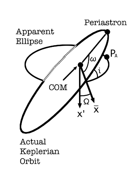
Figure 1: Actual Keplerian orbit and apparent ellipse in three-dimensional space. We denote the inclination angle as $i$, the argument of periastron as $\omega$ and the longitude of ascending node as $\Omega$. These angles relate two coordinates $(x^{\prime},y^{\prime})$ and $(\bar{x},\bar{y})$, both of which choose the origin as the common center of mass. Here, the $x^{\prime}$ axis is taken to lie along the semi-major axis of the apparent ellipse, while the $\bar{x}$-axis is along the direction of the ascending node.

We consider a Kepler orbit, whose semi-major axis, eccentricity, inclination angle, argument of periastron, and longitude of ascending node are $(a_{K},e_{K},i,\omega,\Omega)$ (see Fig. 1). Here, we focus on a binary whose orbital period $P_{K}$ is known by other observations. Angular positions projected onto the celestial sphere are expressed by using the Thiele-Innes elements (Aitken, 1964; Binnendijk, 1960; Roy, 1988).

Let us assume frequent observations of the angular position in the celestial sphere. Namely, we consider a large number of observed points. For such a case, the statistical average expressed as a summation is taken as the temporal average in an integral form as

$$<F>\equiv\frac{1}{T_{obs}}\int_{0}^{T_{obs}}Fdt,$$ (1)

where $<\quad>$ denotes the mean and $T_{obs}$ denotes the total time duration of the observations.

In this paper, we focus on the periodic motion, so that the above expression becomes the integration over several orbital periods. We thus obtain

$$<F> = \frac{1}{JP}\int_{t_{0}}^{t_{0}+JP}Fdt$$ (2)

$$= \frac{1}{P}\int_{t_{0}}^{t_{0}+P}Fdt$$

$$= \frac{1}{2\pi}\int_{0}^{2\pi}F(1-e_{K}\cos u)du,$$

where $J$ is an integer and we used the Kepler equation

$$t=t_{0}+\frac{P_{K}}{2\pi}(u-e_{K}\sin u),$$ (3)

and $dt=P_{K}(1-e_{K}\cos u)du/2\pi$. Here, $u$ and $t_{0}$ denote the eccentric anomaly and the time of periastron passage, respectively.

Let us consider statistical moments. The second and the third moments of the projected position in $(x,y)$ coordinates are useful to determine orbital parameters. They are defined as

$$M_{xx} \equiv <(x-<x>)^{2}>$$ (4)

$$= \frac{1}{2}(\alpha^{2}+\beta^{2})-\frac{1}{4}e_{K}^{2}\alpha^{2},$$

$$M_{yy} \equiv <(y-<y>)^{2}>$$ (5)

$$= \frac{1}{2}(\gamma^{2}+\delta^{2})-\frac{1}{4}e_{K}^{2}\gamma^{2},$$

$$M_{xy} \equiv <(x-<x>)(y-<y>)>$$ (6)

$$= \frac{1}{2}(\alpha\gamma+\beta\delta)-\frac{1}{4}e_{K}^{2}\alpha\gamma,$$

$$M_{xxx} \equiv <(x-<x>)^{3}>$$ (7)

$$= \frac{3}{8}e_{K}\alpha(\alpha^{2}+\beta^{2})-\frac{1}{4}e_{K}^{3}\alpha^{3},$$

$$M_{yyy} \equiv <(y-<y>)^{3}>$$ (8)

$$= \frac{3}{8}e_{K}\gamma(\gamma^{2}+\delta^{2})-\frac{1}{4}e_{K}^{3}\gamma^{3},$$

$$M_{xxy} \equiv <(x-<x>)^{2}(y-<y>)>$$ (9)

$$= \frac{1}{8}e_{K}(3\alpha^{2}\gamma+\beta^{2}\gamma+2\alpha\beta\delta)-\frac{1}{4}e_{K}^{3}\alpha^{2}\gamma,$$

$$M_{xyy} \equiv <(x-<x>)(y-<y>)^{2}>$$ (10)

$$= \frac{1}{8}e_{K}(3\alpha\gamma^{2}+\alpha\delta^{2}+2\beta\gamma\delta)-\frac{1}{4}e_{K}^{3}\alpha\gamma^{2},$$

where observational errors are assumed to vanish at the last equal in each equation, and $\alpha$, $\beta$, $\gamma$, and $\delta$ are the Thiele-Innes type elements defined by (Iwama et al., 2013)

$$\alpha \equiv a_{K}(\cos\omega\cos\Omega-\sin\omega\sin\Omega\cos i),$$ (11)

$$\beta \equiv -b_{K}(\sin\omega\cos\Omega+\cos\omega\sin\Omega\cos i),$$ (12)

$$\gamma \equiv a_{K}(\cos\omega\sin\Omega+\sin\omega\cos\Omega\cos i),$$ (13)

$$\delta \equiv -b_{K}(\sin\omega\sin\Omega-\cos\omega\cos\Omega\cos i),$$ (14)

where $b_{K}=a_{K}\sqrt{1-e_{K}^{2}}$ is the semi-minor axis. The moments $M_{xx},\cdots,M_{xyy}$ are actually observables. For the moments calculation, temporal information of each observed position is smeared by averaging. If positions of a star are measured with sufficiently small observation errors, one can recover the orbital parameters well by the Iwama+ approach (Iwama et al., 2013).

3 Improved Moment Approach

3.1 Observation errors

In the above formalism, we assume that observed points are located on an apparent ellipse. However, position measurements are inevitably associated with observational errors. Therefore, it is very important to take into account observation noises. In this paper, we add Gaussian errors into position measurements as $x\to x+\Delta x$ and $y\to y+\Delta y$, where $\Delta x$ and $\Delta y$ obey Gaussian distributions with a standard deviation $\sigma$. Then, the expected values of the moments are estimated as

$$E(M_{xx}^{(O)}) = M_{xx}^{(T)}+\frac{N-1}{N}\sigma^{2},$$ (15)

$$E(M_{yy}^{(O)}) = M_{yy}^{(T)}+\frac{N-1}{N}\sigma^{2},$$ (16)

$$E(M_{xy}^{(O)}) = M_{xy}^{(T)},$$ (17)

$$E(M_{xxx}^{(O)}) = M_{xxx}^{(T)},$$ (18)

$$E(M_{yyy}^{(O)}) = M_{yyy}^{(T)},$$ (19)

$$E(M_{xxy}^{(O)}) = M_{xxy}^{(T)},$$ (20)

$$E(M_{xyy}^{(O)}) = M_{xyy}^{(T)},$$ (21)

where $N$ is the total number of observed points, and the upper indices $(O)$ and $(T)$ denote observables including observational errors and true values corresponding to Eqs. (4) - (10), respectively. Since $N$ is a large number, $(N-1)/N\simeq 1$. Eqs. (15) and (16) suggest that orbital parameters are not recovered well in the case that $\sigma^{2}$ is comparable to or larger than $M_{xx}$ and $M_{yy}$, even if $N$ approaches the infinity. In this section, we improve the Iwama+ approach to obtain the moments with a higher accuracy for such a large observational errors by incorporating temporal information.

3.2 Averaging operation

By incorporating temporal information, we average the coordinate values of observed points which are neighboring positions. Let us assume that an orbital period of a binary $P_{K}$ is known with high accuracy by another observation, such as observations of absorption lines (e.g., Brocksopp et al. (1999) for Cyg X-1 and Sarty et al. (2011) for LS 5039). If observational errors are so large, neighboring positions on the orbit can be considered as the same position within some errors. In other words, one can identify an observed point at a time $t_{1}$ with another one at a time $t_{2}$ when

$$\frac{\Delta t}{P_{K}}\ll\sigma,$$ (22)

in the units of $a_{K}=1$, where

$$\Delta t=|t_{1}-t_{2}|~{}(\mbox{mod }P_{K}).$$ (23)

Let us divide the apparent ellipse into small bins, each of which corresponds to an equal short time interval, e.g., $[t_{0},t_{0}+P_{K}/n_{m}]$, where $n_{m}$ is the number of the bins. If the same star is observed at fixed intervals, then, every bin has the equal number of observed points $n_{a}=N/n_{m}$ and one obtains more bins near the apastron than near periastron. Namely, every bin will contain the same number of points if and only if the interval between the observations is not a multiple of the bin duration. Note that we can use the data over several orbital periods, so that each bin may include observed points of different orbital periods.

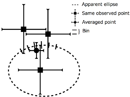
Figure 2: The dashed ellipse is the apparent one, the square and disc with the error bars are observed points and averaged one, respectively. The apparent ellipse is divided by a small bin which has $n_{a}$ observed points. The averaged point approaches the true value if $n_{a}$ is a large number.

In order to reduce statistical errors, we average the positions of $n_{a}$ observed points for each bin and obtain $n_{m}$ averaged points (see Fig. 2). With this averaging operation, the expected values of the moments are given as

$$E(\overline{M}_{xx}^{(O)}) = M_{xx}^{(T)}+\frac{N-1}{N}\frac{\sigma^{2}}{n_{a}},$$ (24)

$$E(\overline{M}_{yy}^{(O)}) = M_{yy}^{(T)}+\frac{N-1}{N}\frac{\sigma^{2}}{n_{a}},$$ (25)

where the bar denotes the value obtained by $n_{m}$ averaged points. Hence, if $n_{a}$ is sufficiently large, the errors of $\overline{M}_{xx}^{(O)}$ and $\overline{M}_{yy}^{(O)}$ could be neglected safely. Therefore, the Iwama+ approach is improved with regard to the accuracy of the moments by the averaging operation.

4 Results

4.1 Numerical test

In Eqs. (1) and (2), we assume that one can integrate observed quantities. In practice, however, observations are discrete, for which the integration should be replaced by a summation. The integration and the summation could agree in the limit that $n_{m}$ approaches the infinity. In addition, it is necessary that $n_{a}$ is so large to reduce errors. According to the numerical calculations, the present approach recovers orbital parameters for $n_{m}=100$ (see the discussion in Iwama et al. (2013) in the absence of the averaging operation, i.e. $n_{a}=1$ & $n_{m}=N$). Therefore, one can use $N/100$ points for the averaging operation on each bin.

For the true parameters $(a_{K},e_{K},i,\omega,\Omega)=(1.0,0.1,30\mathrm{~{}[deg.]},30\mathrm{~{}[deg.]},30\mathrm{~{}[deg.]})$, we consider two cases for $N=10000$. Case 1: the observational error for each position measurement is equal to a binary size, namely, $\sigma=1$ in the units of $a_{K}$. Case 2: $\sigma=5$ in the units of $a_{K}$. For each case, $\sigma/\sqrt{N}$ is fixed where we imagine an instrument, such as the Small-JASMINE. For each parameter set, 100 realizations are done and the mean and the standard deviation are also evaluated.

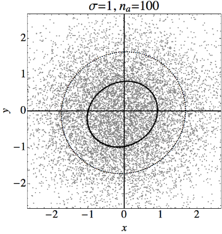
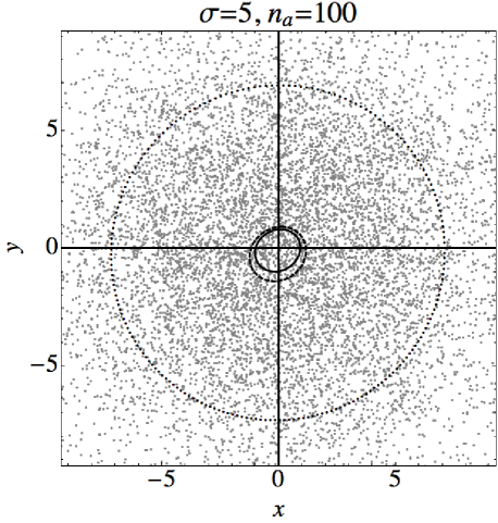
Figure 3: Numerical test: ten thousand observed points of the same source star on the $x-y$ plane. The parameters are $a_{K}=1.0$, $e_{K}=0.1$, $i=30$ [deg.], $\omega=30$ [deg.], $\Omega=30$ [deg.], and $N=10000$ with $n_{a}=100$. The gray points are the observed ones. The solid curve is the apparent ellipse for the true parameters. The dotted and dashed curves denote orbits for the mean value of the recovered parameters by Iwama+ approach and the present one, respectively. Left: $\sigma=1$. Comparison between Iwama+ and the present approaches. Here, the true orbit and the recovered orbit by the present approach overlap each other. Right: $\sigma=5$. Comparison between Iwama+ and the present approaches.

Fig. 3 shows the apparent orbits for the mean values of the recovered parameters by Iwama+ approach and the present one. The present approach can recover the orbital parameters better than the Iwama+ approach. Especially, one can see that the true orbit and the recovered orbit by the present approach almost overlap each other for $\sigma=1$.

Table 1 is a list of orbital parameters that are recovered by the Iwama+ approach and the present approach for $n_{a}=100$, respectively. In both cases, the difference between the true value of the semi-major axis and the mean of the recovered one decreases to less than a tenth. This can be seen in Fig. 3, and is consistent with an order-of-magnitude estimation from Eqs. (24) and (25) (see Appendix A). On the other hand, the dispersion of recovered parameters is not improved by the averaging operation since the order of magnitude of the dispersion depends on not $n_{a}$ but $\sigma/\sqrt{N}$.

In the case 1, the longitude of ascending node is well recovered with the accuracy of less than 10 % of the true value, while the other recovered parameters by the Iwama+ approach are quite different from the true values. By the averaging operation, all of mean recovered values approach the true values. In the case 2, the recovered values except $\omega$ are improved.

Our numerical tests suggest that $\omega$ and $\Omega$ are not always improved by the present approach. However, this point is not important, since the change of the differences between the recovered values of $\omega$ and $\Omega$ and the true values of them are smaller than the dispersion of the recovered values.

In order to confirm the reliability of the above results, we calculate for $16(=2^{4})$ parameter sets as $e_{K}=0.1$ and $0.5$, $i=30$ and $60$ [deg.], $\omega=30$ and $60$ [deg.], and $\Omega=30$ and $60$ [deg.]. One example as $(e_{K},i,\omega,\Omega)=(0.5,60\mathrm{~{}[deg.]},60\mathrm{~{}[deg.]},60\mathrm{~{}[deg.]})$ is added into Table 1 for saving the space. Fourier analyses recover the orbital period from numerically simulated data of the above two cases with the accuracy of $\simeq$ 1 % and 5 %, respectively.

4.2 Possible Application to Cyg X-1

Let us consider a possible application to Cyg X-1, whose angular radius is $\sim 0.03$ milli-arcseconds (mas). The required precision of the Small-JASMINE is $0.01$ mas, so that $\sigma/\sqrt{N}=0.01/0.03\simeq 0.3$. For Cyg X-1, the Small-JASMINE is expected to measure the position of the star with the accuracy of 3 mas, which corresponds to $\sigma=100$, for each imaging. Hence, the position measurements of $N\simeq 10^{5}$ times are required as one data-set for $\sigma/\sqrt{N}\simeq 0.3$.

Since the Small-JASMINE is expected to measure for $3-4$ orbital periods of Cyg X-1, $\simeq 10^{6}$ observed points, which correspond to 10 data-sets, will be obtained. This means that $\sigma/\sqrt{N}\simeq 0.1$ exceeds the required precision of the Small-JASMINE. However, every observed point has the systematic error of the Small-JASMINE as $\sim 0.01$ mas, so that the recovered parameters might also have the error of $\sim 0.01$ mas.

In this paper, we consider two cases as numerical tests where we fix $\sigma/\sqrt{N}$ for each data-set. Case 1: $N=100$, $\sigma=3$, $n_{a}=1$. In this case, the present approach reduces to the Iwama+ one. Case 2: $N=1000$, $\sigma=9.5$, $n_{a}=10$. See Table 2 for a comparison of these cases of one data-set. In the case 2, the present approach recovers the semi-major axis and the inclination better than the Iwama+ one.

On the other hand, the recovered eccentricity by the Iwama+ approach is close to the true value, which is considered to be an accidental coincidence. Numerical calculations of other parameter sets suggest that the recovered eccentricities by the Iwama+ approach and the present one are close to $0.1$ and $0.25$, respectively, for any true eccentricity in the case 2. Hence, the recovered eccentricities by the two approaches may not be reliable when $\sigma/\sqrt{N}=0.3$. For the reliability of the recovered eccentricity, the position measurement with the accuracy of $\sigma/\sqrt{N}=0.01$, which corresponds to the case 1 in the Table 1, is required.

The recovered values by the present approach are comparable to those by the Iwama+ approach for the argument of periastron and the longitude of ascending node. The recovered parameters by the present approach in the case 2 are comparable to the case 1. These numerical results suggest that one can obtain the similar results for $\sigma=3$ and $\sigma=9.5$ by the averaging operation. Hence, the present approach works well to reduce $\sigma$ effectively for $n_{m}=100$.

Next, let us consider the same two cases for 10 data-sets. Table 3 shows the recovered values by the Iwama+ approach and the present approach for 10 data-sets. In both cases, each bin has 10 data-sets of $n_{a}$ observed points, so that $10\times n_{a}$ observed points are effectively averaged in the present approach. On the other hand, every observed point is not averaged in the previous approach.

For the semi-major axis, the mean values of the recovered parameters by the previous approach of 10 data-sets in both cases are comparable to those of one data-set. On the other hand, the recovered semi-major axis by the present approach of 10 data-sets in both cases are much better than those of one data-set.

However, the recovered eccentricities by the both approaches may not be reliable if $\sigma/\sqrt{N}=0.3$ by the similar reason of one data-set. For the reliability of the recovered eccentricity, the position measurement with the accuracy of $\sigma/\sqrt{N}=0.01$, which corresponds to the case 1 in the Table 1, is required. For the inclination, the mean values of the recovered parameters by the present approach are better than those by the previous approach. The recovered values by the present approach are comparable to those by the previous approach for the argument of periastron and the longitude of ascending node. Note that the dispersion of the recovered semi-major axis for 10 data-sets corresponds to random errors of observations. Therefore, the actual observational errors including the systematic errors of the Small-JASMINE will be comparable to the dispersion of Table 2. These results suggest that the semi-major axis of Cyg X-1 is recovered with the accuracy comparable to or smaller than the true value of the semi-major axis by the Small-JASMINE observations. In order to search the best-fit parameter values, recovered values by the present moment approach would work well as trial values in the steepest descent method.

4.3 Comparison with the inversion formula by Asada, Akasaka, and Kasai (2004)

As stated in section 1, Asada, Akasaka, and Kasai (2004) have found an exact solution for orbit determinations of astrometric binaries. The least square method is incorporated into the analytic solution by Asada, Akasaka, and Kudoh (2007). Their numerical calculations show that the analytic method recovers orbital elements for small $\sigma$ cases, such as $\sigma=0.001$ for $N=12$.

We also investigate the averaging operation for the analytic solution (Asada et al., 2004, 2007; Asada, 2008). In the analytic solution, temporal information is fully considered through the law of constant-areal velocity. In addition, one can use more points than $N/100$ for the averaging operations because less than $100$ averaged points are required for the orbit determination differently from the moment approach. Therefore, it seems that the accuracy of the parameter determination by the analytic solution using the averaged points is better than that by the present approach. However, numerical calculations suggest that it is not the case. This is mainly because of two reasons: first, in the analytic solution, parameters of an apparent ellipse must be estimated before the determination of orbital elements, and these parameters can not be recovered well for an extremely low SN ratio. Secondly, the eccentric anomaly $u$ that is needed for calculating areal velocities can not be recovered well. Therefore, recovered values of the orbital elements can be complex numbers or quite different from the true values of them (see Table 4), where complex numbers would suggest hyperbolic orbits rather than elliptic one. Hence, we do not make a further comparison between the present moment approach and the inversion formula method.

5 Conclusion

This paper improved the Iwama+ approach for an extremely low SN ratio, where observational errors are comparable to or larger than a binary size. With avoiding a direct use of the time-consuming Kepler equation, temporal information is taken into account to increase the accuracy of statistical moments. As numerical tests, 100 realizations are done and the mean and the standard deviation are also evaluated. For instance, the difference between the mean of the recovered values of the semi-major axis and the true value of that is decreased to less than a tenth in the case of $10000$ observed points. Therefore, when one has a number of the observed points, the present moment approach significantly improves the previous one for the orbit determinations. For Cyg X-1, the semi-major axis is expected to be recovered with the accuracy comparable to, or smaller than the true value from astrometric observations alone. Although the inversion formula by Asada, Akasaka, and Kasai is also discussed, numerical calculations show that the averaging operation does not work well in the analytic method. It is more convenient to start with values that are recovered by the present moment approach and next use the steepest descent method for finally reaching the best-fit parameter values. It is left as a future work.

We wish to thank the JASMINE science WG member for stimulating conversations. We would be grateful to Y. Sendouda and T. Yano for useful discussions. This work was supported in part (N.G.) by Ministry of Education, Culture, Sports, Science and Technology, Grant-in-Aid for Scientific Research (A), No. 23244034, and in part (K.Y.) by Japan Society for the Promotion of Science, Grant-in-Aid for JSPS Fellows, No. 24108.

Appendix A Estimation of the recovered semi-major axis

Let us estimate the difference between the recovered value and true one for the semi-major axis. Using Eqs. (11) - (14), (4), and (5), Eqs. (15) and (24) are rewritten as

$$E\left(f(e_{K}^{(O)},i^{(O)},\omega^{(O)},\Omega^{(O)})(a_{K}^{(O)})^{2}\right) = f(e_{K}^{(T)},i^{(T)},\omega^{(T)},\Omega^{(T)})(a_{K}^{(T)})^{2}+\frac{N-1}{N}\sigma^{2},$$ (26)

$$E\left(f(\bar{e}_{K}^{(O)},\bar{i}^{(O)},\bar{\omega}^{(O)},\bar{\Omega}^{(O)})(\bar{a}_{K}^{(O)})^{2}\right) = f(e_{K}^{(T)},i^{(T)},\omega^{(T)},\Omega^{(T)})(a_{K}^{(T)})^{2}+\frac{N-1}{N}\frac{\sigma^{2}}{n_{a}},$$ (27)

where

$$f(e_{K},i,\omega,\Omega) \equiv \frac{1}{2}[(\cos\omega\cos\Omega-\sin\omega\sin\Omega\cos i)^{2}+(1-e_{K}^{2})(\sin\omega\cos\Omega+\cos\omega\sin\Omega\cos i)^{2}]$$ (28)

$$-\frac{1}{4}e_{K}^{2}(\cos\omega\cos\Omega-\sin\omega\sin\Omega\cos i)^{2}.$$

In the order-of-magnitude estimation, one can assume that $a_{K}$ and $f(e_{K},i,\omega,\Omega)$ are independent of each other. Hence,

$$E(f(e_{K},i,\omega,\Omega)a_{K}^{2})\simeq E(f(e_{K},i,\omega,\Omega))E(a_{K}^{2}).$$ (29)

In addition, because $e_{K}$ and the trigonometric functions are from $0$ to $1$, one finds $f(e_{K},i,\omega,\Omega)=\mathrm{O}(1)$. Therefore, the expected values of the recovered semi-major axis by the Iwama+ approach and by the present one are expressed approximately as

$$E\left(a_{K}^{(O)}\right) \sim \sqrt{\left(a_{K}^{(T)}\right)^{2}+\sigma^{2}}\geq a_{K}^{(T)}+\sigma,$$ (30)

$$E\left(\bar{a}_{K}^{(O)}\right) \sim \sqrt{\left(a_{K}^{(T)}\right)^{2}+\frac{\sigma^{2}}{n_{a}}}\geq a_{K}^{(T)}+\frac{\sigma}{\sqrt{n_{a}}},$$ (31)

respectively. Eqs. (30) and (31) suggest that the difference between the true value of the semi-major axis and the mean value of the recovered one decreases to nearly $1/\sqrt{n_{a}}$ by the averaging operation. If $n_{a}\geq 100$, this difference decreases to nearly a tenth.

Table 1: Reconstructing two parameter sets of numerical simulations for two different cases by the Iwama+ and the present approaches. In the table, the row $\sigma=0$ indicates true orbital parameters, whereas the rows $\sigma=1$ and $5$ provide the recovered values for adding Gaussian errors ($1$ or $5$ in the units of the true semi-major axis, respectively). The total number of the observed points $N=10000$ and $n_{a}=100$. For each parameter set, 100 realizations are done and the mean and the standard deviation are also evaluated. For the semi-major axis, the difference between the mean of the recovered values and the true value decreases to less than a tenth.

$\sigma$	Approach	$a_{K}$	$e_{K}$	$i$ [deg.]	$\omega$ [deg.]	$\Omega$ [deg.]
$0$		$1.0$	$0.1$	$30$	$30$	$30$
$1$	Iwama+	$1.73\pm 0.01$	$0.030\pm 0.017$	$17.2\pm 1.9$	$36.6\pm 24.7$	$30.9\pm 6.1$
	Present	$1.01\pm 0.01$	$0.103\pm 0.032$	$30.0\pm 2.2$	$29.6\pm 17.8$	$30.2\pm 4.5$
$5$	Iwama+	$7.18\pm 0.04$	$0.027\pm 0.014$	$9.1\pm 2.3$	$44.5\pm 26.7$	$39.9\pm 25.9$
	Present	$1.27\pm 0.07$	$0.203\pm 0.115$	$28.7\pm 7.0$	$49.7\pm 27.3$	$32.3\pm 20.4$
$\sigma$	Approach	$a_{K}$	$e_{K}$	$i$ [deg.]	$\omega$ [deg.]	$\Omega$ [deg.]
$0$		$1.0$	$0.5$	$60$	$60$	$60$
$1$	Iwama+	$1.67\pm 0.01$	$0.054\pm 0.021$	$27.1\pm 1.1$	$42.4\pm 23.6$	$62.5\pm 2.5$
	Present	$1.00\pm 0.03$	$0.469\pm 0.049$	$58.4\pm 1.2$	$58.8\pm 5.5$	$59.9\pm 1.4$
$5$	Iwama+	$7.16\pm 0.04$	$0.029\pm 0.015$	$9.3\pm 2.8$	$43.9\pm 26.5$	$54.4\pm 24.3$
	Present	$1.19\pm 0.09$	$0.282\pm 0.140$	$41.7\pm 7.4$	$53.6\pm 25.7$	$60.4\pm 8.8$

Table 2: Reconstructing the parameters of numerical simulations for two different cases as ($N=100$, $\sigma=3$, $n_{a}=1$) and ($N=1000$, $\sigma=9.5$, $n_{a}=10$) of one data-set. In the table, the row $\sigma=0$ indicates the true orbital parameters, whereas the rows $\sigma=3$ and $9.5$ provide the recovered values for adding Gaussian errors ($3$ or $9.5$ in the units of the true semi-major axis, respectively). For each parameter set, 100 realizations are done and the mean and the standard deviation are also evaluated.

$\sigma$	$N$	Approach	$a_{k}$	$e_{k}$	$i$ [deg.]	$\omega$ [deg.]	$\Omega$ [deg.]
$0$	$100$		$1.0$	$0.1$	$30$	$30$	$30$
$3$	$100$	Iwama+	$4.76\pm 0.41$	$0.285\pm 0.133$	$27.2\pm 8.3$	$51.9\pm 25.0$	$41.4\pm 23.5$
$9.5$	$1000$	Iwama+	$13.77\pm 0.27$	$0.086\pm 0.045$	$15.7\pm 4.3$	$48.0\pm 25.1$	$41.4\pm 27.8$
		Present	$4.78\pm 0.39$	$0.254\pm 0.142$	$28.1\pm 7.3$	$55.3\pm 24.5$	$38.4\pm 24.6$

Table 3: Reconstructing the parameters of numerical simulations for two different cases as ($N=100$, $\sigma=3$, $n_{a}=1$) and ($N=1000$, $\sigma=9.5$, $n_{a}=10$) of 10 data-sets. In the table, the row $\sigma=0$ indicates the true orbital parameters, whereas the rows $\sigma=3$ and $9.5$ provide the recovered values for adding Gaussian errors ($3$ or $9.5$ in the units of the true semi-major axis, respectively). For each parameter set, 100 realizations are done and the mean and the standard deviation are also evaluated.

$\sigma$	$N$	Approach	$a_{k}$	$e_{k}$	$i$ [deg.]	$\omega$ [deg.]	$\Omega$ [deg.]
$0$	$100$		$1.0$	$0.1$	$30$	$30$	$30$
$3$	$100$	Iwama+	$4.43\pm 0.08$	$0.090\pm 0.046$	$15.0\pm 3.8$	$46.3\pm 23.9$	$45.4\pm 25.8$
		Present	$1.77\pm 0.11$	$0.255\pm 0.125$	$26.6\pm 8.0$	$53.1\pm 27.1$	$38.7\pm 24.7$
$9.5$	$1000$	Iwama+	$13.56\pm 0.08$	$0.031\pm 0.016$	$9.1\pm 2.5$	$46.9\pm 27.0$	$43.2\pm 25.7$
		Present	$1.79\pm 0.13$	$0.236\pm 0.137$	$28.0\pm 7.1$	$52.0\pm 23.0$	$35.1\pm 23.1$

Table 4: Reconstructing the parameters for the analytic solution using the averaged points. In the table, the $\sigma=0$ row indicates true orbital parameters, whereas the $\sigma=1$ row provides the mean of the recovered parameters by the inversion formula for $N=100$ observed points. $10$ points are used by the averaging operation for each averaged point, and 100 realization are done. The orbital elements are $a_{k}=1.0$, $e_{k}=0.1$, $i=30$[deg.], $\omega=30$[deg.], and $\Omega=30$[deg.], respectively.

$\sigma$	$N$	$a_{k}$	$e_{k}$	$i$ [deg.]	$\omega$ [deg.]	$\Omega$ [deg.]
$0$	$100$	$1.0$	$0.1$	$30$	$30$	$30$
$1$	$100$	$3.06$	$13.065$	$78.7+17.0i$	$7.5+0.8i$	$51.3$

References

- Aitken (1964) Aitken, R. G. 1964 The Binary Stars (NY: Dover)
- Asada et al. (2004) Asada, H., Akasaka, T., & Kasai, M. 2004, PASJ, 56, L35
- Asada et al. (2007) Asada, H. Akasaka, T., & Kudoh, K. 2007, AJ, 133, 1243
- Asada (2008) Asada, H. 2008, PASJ, 60, 843
- Binnendijk (1960) Binnendijk, L. 1960 Properties of Double Stars (Philadelphia: University of Pennsylvania Press)
- Brocksopp et al. (1999) Brocksopp, C., Tarasov, A. E., Lyuty, V. M., & Roche, P. 1999, A & A, 343, 861
- Catovic and Olevic (1992) Catovic, Z., & Olevic, D. 1992 in IAU Colloquium 135, ASP Conference Series Vol. 32 (eds McAlister H. A., Hartkopf W. I., ) 217-219 (San Francisco, Astronomical Society of the Pacific)
- Danby (1988) Danby, J. M. A., 1988 Fundamentals of Celestial Mechanics (VA: William-Bell)
- Eichhorn and Xu (1990) Eichhorn, H. K., & Xu, Y. 1990, ApJ, 358, 575
- Gouda et al. (2007) Gouda, N. et al. 2007, Advances in Space Research, 40, 664
- Iwama et al. (2013) Iwama, H., Asada, H., & Yamada, K. 2013, PASJ, 65, 2
- Mignard (2004) Mignard, F. ‘Overall Science Goals of the Gaia Mission’, Proc. The Three-Dimensional Universe with Gaia, 4-7 October 2004, Paris (Netherlands: ESA Publications)
- Olevic and Cvetkovic (2004) Olevic, D., & Cvetkovic, Z. 2004, A&A, 415, 259
- Perryman (2004) Perryman, M. A. C. ‘Overview of the Gaia Mission’, Proc. The Three-Dimensional Universe with Gaia, 4-7 October 2004, Paris (Netherlands: ESA Publications)
- Roy (1988) Roy, A. E. 1988 Orbital Motion (Bristol: Institute of Physics Publishing)
- Sarty et al. (2011) Sarty, G. E. et al. 2011, Mon. Not. R. Astron. Soc., 1293, 411
- Thiele (1883) Thiele, T. N. 1883, Astron. Nachr., 104, 245