AC Josephson effect without superconductivity

Abstract

Superconductivity derives its most salient features from the coherence of its macroscopic wave function. The associated physical phenomena have now moved from exotic subjects to fundamental building blocks for quantum circuits such as qubits or single photonic modes. Here, we theoretically find that the AC Josephson effect—which transforms a DC voltage $V_{b}$ into an oscillating signal $cos(2eV_{b}t/\hbar)$—has a mesoscopic counterpart in normal conductors. We show that on applying a DC voltage $V_{b}$ to an electronic interferometer, there exists a universal transient regime where the current oscillates at frequency $eV_{b}/h$. This effect is not limited by a superconducting gap and could, in principle, be used to produce tunable AC signals in the elusive $0.1-10$ THz “terahertz gap”.

Superconductivity, a macroscopic quantum state, is described by a wave function whose phase is physically significant. Indeed, quantum mechanical interference effects are ubiquitous in superconducting systems, similar to those observed at the microscopic scale in atomic physics. Since the eighties, such effects have also been also observed at the mesoscopic (or nano) scale in condensed matter. Most of the peculiar effects observed in superconductors have an analogue in “normal” quantum nanoelectronics: the DC SQUID (superconducting quantum interference device) corresponds to the Aharonov-Bohm effect Batelaan and Tonomura (2009), supercurrents (at the origin of the Meissner effect) correspond to the so-called persistent currents Imry (2002); Lévy et al. (1990); Castellanos-Beltran et al. (2013). The AC Josephson effect in superconductors is perhaps the most striking manifestation of these interference effects at a macroscopic scale Josephson (1962); a DC voltage bias $V_{b}$ applied across a weak link between two superconductors creates an oscillating current with frequency $2eV_{b}/h$. This voltage to frequency conversion is used in metrology to define the Volt in terms of the Second Parker et al. (1967), as well as in a wealth of superconducting devices (RF-SQUIDs, quantum bits) Devoret and Schoelkopf (2013). Its origin is rather straightforward. The energy of the left superconductor is $eV_{b}$ higher than the right one, so that its wave function gets an extra oscillating factor $e^{-i2eV_{b}t/\hbar}$. The junction produces an interference between these two wave functions, hence the oscillations. The absence of a corresponding mesoscopic effect in normal conductors is in itself surprising from a theoretical perspective; superconductivity is well described by the Bogoliubov-De Gennes equation Gennes (1999), a simple extension of the Schrödinger equation. Here we report on this missing effect. We find that an oscillating signal $\cos(eV_{b}t/\hbar)$ is generated in the transient regime that follows an abrupt change of the bias voltage applied to a normal conductor.

Our story begins with a—two path—electronic Mach-Zehnder interferometer,

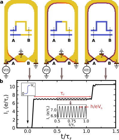
Figure 1: Raising the DC voltage bias on a Mach-Zehnder interferometer in the quantum Hall regime. (a) Colour plot of the local electronic charge density (measured from equilibrium) in a 3 terminal Mach-Zehnder interferometer in the quantum Hall regime: from vanishing density (yellow), to $10^{11}cm^{-2}$ (red). At $t=0$, the voltage bias is raised from $V(t<0)=0$ to $V_{b}=20h/(e\tau_{F})$. The three colour plots correspond to three snapshots for different times as indicated by the arrows. A two-dimensional electron gas (yellow) is connected to three electrodes, the semi-transparent quantum point contacts A and B act as beamsplitters. Insets: schematics of the propagation of the voltage bias along the two arms of the interferometer. (b) Transmitted current at contact 1. Upper inset: schematic of the raising of the bias voltage. Lower inset: zoom on the oscillations of the current.

sketched in Fig. 1a. This device, implemented in a two-dimensional gas under high magnetic field, has lately become a rather standard tool of the mesoscopic physicist Ji et al. (2003); Roulleau et al. (2008). In the quantum Hall regime the bulk of the electronic gas is insulating and the electronic propagation only occurs on the edges of the sample. One can realize electronic beam splitters with quantum point contacts, and in this way ensure that only two paths are available for any travelling electrons. The sample is very asymmetric, the upper arm being much longer than the lower one, which implies an extra time of flight $\tau_{F}=L/v_{g}$ (with $L$ the extra length of the upper arm with respect to the lower one and $v_{g}$ the group velocity of the edge state). At $t=0$ one raises the bias voltage applied on contact $0$ from $V(t<0)=0$ to $V(t>\tau_{P})=V_{b}$. While the exact manner in which the voltage is raised is unimportant, the rise time $\tau_{P}$ must be sufficiently fast ($\tau_{P}<\tau_{F}$), and the voltage drop spatially sharp enough (compared to $L$) Gaury et al. (2014); Gaury and Waintal (2014). Fig. 1b shows the transmitted current $I_{1}(t)$ as a function of time $t$, and we can discern three distinct regimes. In the beginning (Fig. 1a left) the voltage pulse did not have enough time to propagate up to contact $1$, and $I_{1}(t)=0$. During a transient regime of duration $\tau_{F}$ (Fig. 1a middle), the pulse has arrived at contact $1$ from the lower arm but not yet from the upper one. The current increases to a finite value. Finally (Fig. 1a right), the pulse arrives from the upper arm and the current increases to its stationary value. The most noteworthy feature of Fig. 1b lies in the transient regime; the current oscillates with frequency $eV_{b}/h$ around a DC component. This transient oscillatory regime is the mesoscopic analogue of the AC Josephson effect. It is to the AC Josephson effect what persistent currents Imry (2002) are to supercurrents.

The theory required to obtain this transient oscillatory regime is fundamentally simple. Within the time-dependent scattering approach Gaury et al. (2014), one finds that the wave function close to contact $0$ is a plane wave that acquires an additional phase when the bias voltage is raised,

$$\Psi_{0}(x,t)=\frac{1}{\sqrt{k}}e^{ikx-iEt/\hbar-ieV_{b}t\theta(t-x/v_{g})/\hbar}$$ (1)

where $\theta(x)$ is the Heaviside function, $E$ is the incident energy of the electron, $k$ the corresponding momentum, and the curved coordinate $x$ follows the edge of the sample. We have assumed for simplicity a linear dispersion relation $E(k)=\hbar v_{g}k$ and the condition $\tau_{P}\ll\tau_{F}$. We see from Eq. (1) that raising the voltage induces an oscillating phase difference $e^{ieV_{b}t/\hbar}$ between the front and the rear of the wave. One can consider this phase difference as the time-dependent extension of the stationary case that was discussed in Levitov et al. (1996); Gaury and Waintal (2014). The device uses the delay time $\tau_{F}$ between the two arms to create an interference between the rear and the front of the wave function, generating the oscillatory behavior. In the transient regime, the wave function close to contact $1$ is the superposition of the contributions from the two paths and one finds,

$$\Psi_{1}(x,t)=\frac{e^{ikx-iEt/\hbar}}{\sqrt{k}}d_{1}(t,E)$$ (2)

with the total time-dependent transmission amplitude $d_{1}(t,E)$ given by,

$$d_{1}(t,E)=d_{u}(E)e^{-iE\tau_{F}/\hbar}+d_{l}(E+eV_{b})e^{-ieV_{b}t/\hbar}$$ (3)

The amplitudes $d_{u/l}$ for the upper/lower arm are given in terms of the transmission probabilities $T_{A/B}$ of the quantum point contacts, $d_{u}=\sqrt{T_{A}T_{B}}$ and $d_{l}=\sqrt{(1-T_{A})(1-T_{B})}$. Using the time-dependent generalization of the Landauer formula Gaury et al. (2014),

$$I_{1}(t)=(e/h)\int dE|d_{1}(t,E)|^{2}f(E)$$ (4)

[$f(E)$ is the Fermi function, Eq. (4) includes the equilibrium current injected from contact 0 which needs to be subtracted], we finally get the current at contact 1 during the transient regime,

$$I_{1}(t)= \frac{e^{2}V_{b}}{h}T_{A}T_{B}$$

$$+\frac{e}{\pi\tau_{F}}\sqrt{T_{A}T_{B}(1-T_{A})(1-T_{B})}\cos\left(\frac{eV_{b}t}{\hbar}+\phi\right)$$ (5)

Eq. (AC Josephson effect without superconductivity) is the main result of this letter and agrees with the direct microscopic numerical calculations presented above. While the precise coefficients depend on the particular interferometer considered, its structure is totally general. It contains a DC term plus an AC term at frequency $eV_{b}/h$; the amplitude of the AC current is of the order of $e/\tau_{F}$. For a typical micrometer sized Mach-Zehnder interferometer, the amplitude of the AC current is of the order of a few nA.

The Mach-Zehnder interferometer is simple conceptually, but challenging experimentally in terms of the lithography (for the central electrode $2$), low temperature and high magnetic field.

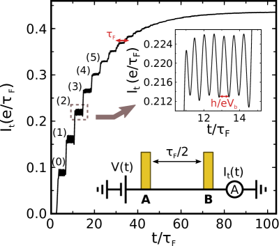
Figure 2: Raising the DC voltage bias on a Fabry-Perot interferometer. Transmitted current (in units of $e/\tau_{F}$, where $\tau_{F}$ is twice time of flight between the two barriers) as a function of time for a Fabry-Perot cavity. At $t=0$, the voltage bias is raised from $V(t<0)=0$ to $V_{b}=6h/(e\tau_{F})$. Upper inset: zoom on the oscillations of the current on a plateau. Lower inset: schematic of the Fabry-Perot cavity ($T_{a}=T_{b}=0.1$).

Fabry-Perot cavities, in contrast, are ubiquitous and occur every time two barriers are put in series. Examples include carbon nanotubes Liang et al. (2001), quantum Hall systems van Wees et al. (1989) and semi-conducting nanowires Kretinin et al. (2010). Fig. 2 shows a sketch of the Fabry-Perot geometry together with a numerical calculation of the measured current as a function of time. The $I_{t}(t)$ curve now features many steps that correspond to the arrival of the path with direct transmission (0), the path with one reflection on B and A (1), two reflections (2) and so on. Again, each of these steps is accompanied by oscillations at the frequency $eV_{b}/h$. On decreasing the transparencies of the barriers, $T_{A}$ and $T_{B}$, the Fabry-Perot resonances gradually become true bound states and the duration of the transient regime increases accordingly. This situation is very close, mathematically, to the true Andreev bound states that occur in a Josephson junction Beenakker and van Houten (1991).

Experimentally, progress in ultrafast quantum transport has been steady with the recent demonstration of single electron sources resolved in energy Fève et al. (2007) or time Dubois et al. (2013) as well as measurements in the THz range Zhong et al. (2008). For an easier observation of the transient AC signal, it might be convenient to replace the abrupt voltage change described above by a train of square pulses (with a “slow” period $\sim\tau_{F}$) as produced by, say, ring oscillators. Such a train of pulses would stabilize the AC signal and should permit its observation with current technology. The transient AC regime is however not restricted to well defined interferometers and could be observed in any situation where the electronic transport is coherent. One could consider using multichannel systems such as small pillars of metallic multilayers (with metal–metal interfaces acting as the barriers), or the universal conductance fluctuations of disordered metals. The corresponding signals from the different channels/set of interfering trajectories would be added incoherently in such systems which would lead to a sharp peak at the frequency $eV_{b}/h$ in the current noise. In contrast to its superconducting counterpart, the AC frequency predicted here is not limited by a superconducting gap, meaning that high frequencies can be obtained. The effect could possibly be used to make tunable radiofrequency sources that go beyond the GHz regime.

Methods
Numerical method. The time-dependent numerical calculations have been performed using the T-Kwant algorithm described in Gaury et al. (2014), following the model detailed in Gaury and Waintal (2014). The DC calculations were performed with the Kwant open source package Groth et al. (2014).

Acknowledgements
This work was supported by the ERC grant MesoQMC from the European Union. We thank J.-P. Brison for careful reading of the manuscript and useful comments.

Author contributions
X.W. initiated the project. B.G. and J.W. performed the numerical simulations. X.W., B.G. and J.W. performed the analytical calculations, data analysis and wrote the manuscript.

Contact information
Correspondence and requests for materials should be addressed to X.W. (email: xavier.waintal@cea.fr)

References

- Batelaan and Tonomura (2009) A. Batelaan and A. Tonomura, Physics Today 62, 38 (2009).
- Imry (2002) Y. Imry, Introduction to mesoscopic physics (Oxford University Press, 2002), 2nd ed.
- Lévy et al. (1990) L. P. Lévy, G. Dolan, J. Dunsmuir, and H. Bouchiat, Phys. Rev. Lett. 64, 2074 (1990).
- Castellanos-Beltran et al. (2013) M. A. Castellanos-Beltran, D. Q. Ngo, W. E. Shanks, A. B. Jayich, and J. G. E. Harris, Phys. Rev. Lett. 110, 156801 (2013).
- Josephson (1962) B. D. Josephson, Physics Letters 1, 251 (1962).
- Parker et al. (1967) W. H. Parker, B. N. Taylor, and D. N. Langenberg, Phys. Rev. Lett. 18, 287 (1967).
- Devoret and Schoelkopf (2013) M. H. Devoret and R. J. Schoelkopf, Science 339, 1169 (2013).
- Gennes (1999) P. G. D. Gennes, Superconductivity Of Metals And Alloys (Westview Press, 1999).
- Ji et al. (2003) Y. Ji, Y. Chung, D. Sprinzak, M. Heiblum, D. Mahalu, and H. Shtrikman, Nature 422, 415 (2003).
- Roulleau et al. (2008) P. Roulleau, F. Portier, P. Roche, A. Cavanna, G. Faini, U. Gennser, and D. Mailly, Phys. Rev. Lett. 100, 126802 (2008).
- Gaury et al. (2014) B. Gaury, J. Weston, M. Santin, M. Houzet, C. Groth, and X. Waintal, Physics Reports 534, 1 (2014).
- Gaury and Waintal (2014) B. Gaury and X. Waintal, Nat. Commun. 5 (2014).
- Levitov et al. (1996) L. S. Levitov, H. Lee, and G. B. Lesovik, Journal of Mathematical Physics 37, 4845 (1996).
- Liang et al. (2001) W. Liang, M. Bockrath, D. Bozovic, J. H. Hafner, M. Tinkham, and H. Park, Nature 411, 665 (2001).
- van Wees et al. (1989) B. J. van Wees, L. P. Kouwenhoven, C. J. P. M. Harmans, J. G. Williamson, C. E. Timmering, M. E. I. Broekaart, C. T. Foxon, and J. J. Harris, Phys. Rev. Lett. 62, 2523 (1989).
- Kretinin et al. (2010) A. Kretinin, R. Popovitz-Biro, D. Mahalu, and H. Shtrikman, Nano Letters 10, 3439 (2010).
- Beenakker and van Houten (1991) C. W. J. Beenakker and H. van Houten, Phys. Rev. Lett. 66, 3056 (1991).
- Fève et al. (2007) G. Fève, A. Mahé, J.-M. Berroir, T. Kontos, B. Plaçais, D. C. Glattli, A. Cavanna, B. Etienne, and Y. Jin, Science 316, 1169 (2007).
- Dubois et al. (2013) J. Dubois, T. Jullien, F. Portier, P. Roche, A. Cavanna, Y. Jin, W. Wegscheider, P. Roulleau, and D. C. Glattli, Nature 502, 659 (2013).
- Zhong et al. (2008) Z. Zhong, N. M. Gabor, J. E. Sharping, A. Gaetal, and P. L. McEuen, Nature Nanotechnology 3, 201 (2008).
- Groth et al. (2014) C. W. Groth, M. Wimmer, A. R. Akhmerov, and X. Waintal, New J. Phys. 16, 063065 (2014).