Statistical tests of sterile neutrinos using cosmology and short-baseline data

Abstract

In this paper we revisit the question of the information which cosmology provides on the scenarios with sterile neutrinos invoked to describe the SBL anomalies using Bayesian statistical tests. We perform an analysis of the cosmological data in $\Lambda$CDM$+r+\nu_{s}$ cosmologies for different cosmological data combinations, and obtain the marginalized cosmological likelihood in terms of the two relevant parameters, the sterile neutrino mass $m_{s}$ and its contribution to the energy density of the early Universe $\Delta N_{\text{\rm eff}}$. We then present an analysis to quantify at which level a model with one sterile neutrino is (dis)favoured with respect to a model with only three active neutrinos, using results from both short-baseline experiments and cosmology. We study the dependence of the results on the cosmological data considered, in particular on the inclusion of the recent BICEP2 results and the SZ cluster data from the Planck mission. We find that only when the cluster data is included the model with one extra sterile neutrino can become more favoured that the model with only the three active ones provided the sterile neutrino contribution to radiation density is suppressed with respect to the fully thermalized scenario. We have also quantified the level of (in)compatibility between the sterile neutrino masses implied by the cosmological and SBL results.

1 Introduction

It is now an established fact that neutrinos are massive and leptonic flavors are not symmetries of Nature Pontecorvo:1967fh ; Gribov:1968kq . In the last decade this picture has become fully established thanks to the upcoming of a set of precise experiments. In particular, the results obtained with solar and atmospheric neutrinos have been confirmed in experiments using terrestrial beams GonzalezGarcia:2007ib . The minimum joint description of all these data requires mixing among all the three known neutrinos ($\nu_{e}$, $\nu_{\mu}$, $\nu_{\tau}$), which can be expressed as quantum superposition of three massive states $\nu_{i}$ ($i=1,2,3$) with masses $m_{i}$ leading to the observed oscillation signals with $\Delta m^{2}_{21}=(7.5^{+0.19}_{-0.17})\times 10^{-5}$ eV² and $|\Delta m^{2}_{31}|=(2.458\pm 0.002)\times 10^{-3}$ eV² and non-zero values of the three mixing angles GonzalezGarcia:2012sz .

In addition to these well-established results, there remains a set of anomalies in neutrino data at relatively short-baselines (SBL) (see Ref. Abazajian:2012ys for a review) including the LSND LSND:2001ty and MiniBooNE  MiniBooNE:2010wv ; Aguilar-Arevalo:2013pmq observed $\nu_{\mu}\rightarrow\nu_{e}$ transitions, and the $\bar{\nu}_{e}$ disappearance at reactor Mention:2011rk ; Mueller:2011nm ; Huber:2011wv and Gallium Giunti:2010zu ; Giunti:2012tn ; Acero:2007su experiments. If interpreted in terms of oscillations, each of these anomalies points out towards a $\Delta m^{2}\sim{\cal O}({\rm eV}^{2})$  Kopp:2011qd ; Giunti:2011gz ; Giunti:2011hn ; Giunti:2011cp ; Donini:2012tt ; Conrad:2012qt ; Giunti:2013aea ; Karagiorgi:2012kw ; Kopp:2013vaa and consequently cannot be explained within the context of the 3$\nu$ mixing described above. They require instead the addition of one or more neutrino states which must be sterile, i.e. elusive to Standard Model interactions, to account for the constraint of the invisible $Z$ width which limits the number of light weak-interacting neutrinos to be $2.984\pm 0.008$ Nakamura:2010zzi .

Several combined analyses have been performed to globally account for these anomalies in addition to all other oscillation results in the context of models with one or two additional sterile neutrinos Giunti:2013aea ; Karagiorgi:2012kw ; Conrad:2012qt ; Kopp:2013vaa with somehow different conclusions in what respects to the possibility of a successful joint description of all the data. Generically these global fits reveal a tension between disappearance and appearance results. But while Refs. Giunti:2013aea ; Karagiorgi:2012kw seem to find a possible compromise solution for 3+1 mass schemes, the analysis in Ref. Kopp:2013vaa concludes a significantly lower level of compatibility. In particular, Ref. Giunti:2013aea concludes that a joint solution is found with

$$0.82\leq\Delta m^{2}_{41}\leq 2.19\;{\rm eV}^{2}\;\;{\rm at}\rm\;\;3\sigma$$ (1)

$$|U_{e4}|^{2}\sim 0.03\,,\;\;\;|U_{\mu 4}|^{2}\sim 0.012\;.$$

Alternative information on the presence of light sterile neutrinos is provided by Cosmology as they contribute as extra radiation to the energy density of the early Universe which can be expressed as

$$\rho_{R}=\left[1+\frac{7}{8}\left(\frac{4}{11}\right)^{4/3}N_{\rm eff}\right]\rho_{\gamma}\,,$$ (2)

where $\rho_{\gamma}$ is the photon energy density and the value of $N_{\rm eff}$ in the Standard Model (SM) is equal to $N_{\rm eff}^{\rm SM}=3.046$ Mangano:2005cc . The presence of extra radiation is then usually quantified in terms of the parameter $\Delta N_{\rm eff}\equiv N_{\rm eff}-N^{\rm SM}_{\rm eff}$.

Sterile neutrinos contribute to $\rho_{R}$ (i.e. to $\Delta N_{\rm eff}$) in a quantity which, in the absence of other forms of new physics, is a function of their mass and their mixing with the active neutrinos which determines to what degree they are in thermal equilibrium with those. In particular, in $3+N_{s}$ scenarios with the values hinted by the SBL results (of the order of those in Eq. (1)) the sterile neutrinos are fully thermalized (FT) and each one contributes to $\rho_{R}$ as much as an active one (see for example Saviano:2013ktj ; Mirizzi:2013kva ), so

$$\Delta N^{3+N_{s},FT}_{\rm eff}=N_{s}\>.$$ (3)

Analyses of cosmological data have hinted for the presence of extra radiation, beyond the standard three active neutrinos since several years (see for example Ref. GonzalezGarcia:2010un and references therein) and several authors have invoked the presence of eV-scale sterile neutrino as a plausible source of the extra radiation  Acero:2008rh ; Hamann:2010bk ; Giusarma:2011zq ; Archidiacono:2011gq ; Archidiacono:2012ri . In the last four years the statistical significance of this extra radiation (or its upper bound) as well as the overall constraint on the neutrino mass scale has been changing as data from the Planck satellite Ade:2013lta , the Atacama Cosmology Telescope (ACT)  Das:2013zf , the South Pole Telescope (SPT)  Keisler:2011aw ; Reichardt:2011yv , and most recently of the BICEP2 Ade:2014xna experiment, has become available  Verde:2013cqa ; Archidiacono:2014apa ; Dvorkin:2014lea ; Zhang:2014dxk ; Zhang:2014nta ; Wu:2014qxa ; Leistedt:2014sia ; Giusarma:2014zza .

In particular, the recent measurement of B-mode signals from the BICEP2 Ade:2014xna collaboration excludes a zero scalar-to-tensor ratio at $7\sigma$ and report a value of $r=0.20^{+0.07}_{-0.05}$. This high value of $r$ is compatible with previous results from the Planck data Ade:2013lta if a running of the scalar spectral index $dn_{s}/d\ln k$ is considered well beyond the characteristic value of $10^{-4}$ of slow-roll inflation models. Alternatively the tension might be eased by the presence of sterile neutrinos Archidiacono:2014apa ; Dvorkin:2014lea ; Zhang:2014dxk ; Zhang:2014nta ; Wu:2014qxa without invoking such a large running of the scalar spectral index.

Since cosmological data have the potential to test regions of parameter space of the sterile neutrino scenarios invoked to account for the SBL anomalies, the question of to what degree they support them has received an increasing attention in the literature Hamann:2011ge ; Archidiacono:2012ri ; Kristiansen:2013mza ; Archidiacono:2013xxa ; Gariazzo:2013gua . The generic conclusion is that, in order to accommodate the cosmological observations within the $3+N_{s}$ scenarios motivated by SBL results, some new form of physics is required to suppress the contribution of the sterile neutrinos to the radiation component of the energy density at the CMB epoch with respect to the FT expectation Eq. (3). Among others extended scenarios with a time varying dark energy component Giusarma:2011zq , entropy production after neutrino decoupling Ho:2012br , very low reheating temperature Gelmini:2004ah , large lepton asymmetry Foot:1995bm ; Chu:2006ua ; Saviano:2013ktj , and non-standard neutrino interactions  Bento:2001xi ; Dasgupta:2013zpn ; Hannestad:2013ana , have been considered. All these mechanisms have the effect of diluting the sterile neutrino abundance or suppressing the production in the early Universe.

In this paper we revisit the question of the information which cosmology provides on the sterile scenarios introduced to explain the SBL anomalies using precise Bayesian statistical tests which we briefly describe in Sec. 2. Section 3 contains the results of our cosmological analysis in $\Lambda$CDM$+r+\nu_{s}$ cosmologies for three representative sets of cosmological data. With these results at hand we answer the question of how much cosmological data favour or disfavour the scenario with sterile neutrino masses invoked by SBL anomalies, with respect to a model without sterile neutrinos? in Sec. 4, and we do so in terms of the departure from the fully thermalized expectation, Eq. (3). We also discuss the consistency of sterile parameter constrains implied by cosmology and SBL. In Sec. 5 we summarize our conclusions.

2 The statistical framework

2.1 Model comparison

Bayesian inference is a rigorous framework for inferring which, out of set of models or hypotheses $H_{i}$, are favoured by a data set $\mathbf{D}$. Bayes’ theorem is used to calculate the probabilities of each of the hypotheses after considering the data, the posterior probabilities,

$$\Pr(H_{i}|\mathbf{D})=\frac{\Pr(\mathbf{D}|H_{i})\Pr(H_{i})}{\Pr(\mathbf{D})}.$$ (4)

Here $\Pr(\mathbf{D}|H_{i})$ is the probability of the data, assuming the model $H_{i}$ to be true, while $\Pr(H_{i})$ is the prior probability of $H_{i}$, which is how plausible $H_{i}$ is before considering the data. Considering especially the case of a discrete set of models, one can compare two of them by calculating the ratio of posterior probabilities, the posterior odds, as

$$\mathcal{O}_{ij}=\frac{\Pr(H_{i}|\mathbf{D})}{\Pr(H_{j}|\mathbf{D})}=\frac{\Pr(\mathbf{D}|H_{i})}{\Pr(\mathbf{D}|H_{j})}\frac{\Pr(H_{i})}{\Pr(H_{j})}=B_{ij}\frac{\Pr(H_{i})}{\Pr(H_{j})}.$$ (5)

In words, the posterior odds is given by the prior odds $\Pr(H_{i})/\Pr(H_{j})$ multiplied by the Bayes factor $B_{ij}=\Pr(\mathbf{D}|H_{i})/{\Pr(\mathbf{D}|H_{j})}$, which quantifies how much better $H_{i}$ describes that data than $H_{j}$. The prior odds quantifies how much more plausible one model is than the other a priory, i.e., without considering the data. If there is no reason to favour one of the models over the other, the prior odds equals unity, in which case the posterior odds equals the Bayes factor.

For a model $H$, containing the continuous free parameters $\mathbf{\Theta}$, $\Pr(\mathbf{D}|H)$ also called evidence of the model is given by

$$\Pr(\mathbf{D}|H) =$$

$$\int\Pr(\mathbf{D},\mathbf{\Theta}|H){\rm d}^{N}\mathbf{\Theta} = \int\Pr(\mathbf{D}|\mathbf{\Theta},H)\Pr(\mathbf{\Theta}|H){\rm d}^{N}\mathbf{\Theta}$$ (6)

$$= \int{\mathcal{L}(\mathbf{\Theta})\pi(\mathbf{\Theta})}{\rm d}^{N}\mathbf{\Theta}.$$

Here, the likelihood function $\Pr(\mathbf{D}|\mathbf{\Theta},H)$ is the probability (density) of the data as a function of the assumed free parameters, which we often denote by $\mathcal{L}(\mathbf{\Theta})$ for simplicity. The quantity $\Pr(\mathbf{\Theta}|H)$ is the correctly normalized prior probability (density) of the parameters and is often denoted by $\pi(\mathbf{\Theta})$. The assignment of priors is often far from trivial, but an important part of a Bayesian analysis.

From Eq. (6), we note that the evidence is the average of the likelihood over the prior, and hence this method automatically implements a form of Occam’s razor, since usually a theory with a smaller parameter space will have a larger evidence than a more complicated one, unless the latter can fit the data substantially better.

Bayes factors, or rather posterior odds, are usually interpreted or “translated” into ordinary language using the so-called Jeffreys scale, given in Tab. 1, where “$\log$” is the natural logarithm. This has been used in applications such as Refs. Trotta:2008qt ; Hobson:2010book ; Feroz:2008wr (and Refs. Bergstrom:2012yi ; Bergstrom:2012nx in neutrino physics), although slightly more aggressive scales have been used previously Jeffreys:1961 ; Kass:1995 .

$|\log(\text{odds})|$	odds	$\Pr(H|\mathbf{D})$	Interpretation
$<1.0$	$\lesssim 3:1$	$\lesssim 0.75$	Inconclusive
$1.0$	$\simeq 3:1$	$\simeq 0.75$	Weak evidence
$2.5$	$\simeq 12:1$	$\simeq 0.92$	Moderate evidence
$5.0$	$\simeq 150:1$	$\simeq 0.993$	Strong evidence

Table 1: Jeffrey’s scale often used for the interpretation of model odds. The posterior model probabilities for the preferred model $H$ are calculated by assuming only two competing hypotheses.

2.2 Parameters of interest and the marginal likelihood

In Bayesian statistics if one assumes a particular parametrized model to be correct, the complete inference of the parameters of that model is given by the posterior distribution through Bayes’ theorem

$$\Pr(\mathbf{\Theta}|\mathbf{D},H)=\frac{\Pr(\mathbf{D}|\mathbf{\Theta},H)\Pr(\mathbf{\Theta}|H)}{\Pr(\mathbf{D}|H)}=\frac{\mathcal{L}(\mathbf{\Theta})\pi(\mathbf{\Theta})}{\Pr(\mathbf{D}|H)}.$$ (7)

We see that the evidence here appears as a normalization constant in the denominator. Since the evidence does not depend on the values of the parameters $\mathbf{\Theta}$, it is usually ignored in parameter estimation problems and the parameter inference is obtained using the unnormalized posterior.

For the case in which we have a only a subset of parameters of interest, $\lambda$, so $\mathbf{\Theta}=(\lambda,\eta)$, where $\eta$ denotes the nuisance parameters,

$$P(\lambda,\eta)=\Pr(\lambda,\eta|\mathbf{D},H)\propto\mathcal{L}(\lambda,\eta)\pi(\lambda,\eta)\,,$$ (8)

and inference on $\lambda$ is obtained by marginalizing over the nuisance parameters in the usual way

$$P(\lambda)=\int P(\lambda,\eta){\rm d}\eta\,,$$ (9)

with no need to ever consider a likelihood $\mathcal{L}(\lambda)$ depending only on the parameter of interest. This is typically unproblematic in the case where the data is sufficiently informative to eliminate all practical prior dependence. Often, however, this is not the case, and there can be large dependence on the prior chosen. In this case one can consider as a partial step the marginal likelihood function

$$\mathcal{L}(\lambda)=\int\mathcal{L}(\lambda,\eta)\pi(\eta){\rm d}\eta\,,$$ (10)

such that $P(\lambda)\propto\mathcal{L}(\lambda)\pi(\lambda).$

This likelihood function then encodes the information on $\lambda$ contained in the data (under $H$ and after taking into account the uncertainty on the nuisance parameters), without needing to specify a prior $\pi(\lambda)$. Note that, since the marginal likelihood is not a probability density, it is not normalized to unity, and is not sufficient to perform the full inference. Also, it is generally different from the profile likelihood, so regions defined by $-2\log(\mathcal{L}(\lambda)/\mathcal{L}^{\rm max})<C$ will not, in general, be the same as those using the profile likelihood, although arguments justifying defining regions in this way for profile likelihoods typically also apply to marginal likelihoods. As shown in Ref. Planck:2013nga , the profile and marginal likelihoods are indeed similar for the cosmological data and models considered there. In any case, the marginal likelihood can still be useful in scientific reporting as a rough guide to what information the data contains, for example, by considering regions defined by $-2\log(\mathcal{L}(\lambda)/\mathcal{L}^{\rm max})<C$ berger1999 .

Furthermore, if two data sets do not share any common nuisance parameters, the two marginal likelihoods can simply be multiplied to obtain the total marginal likelihood. Notice, however, that the marginal likelihood still depends on the priors on the nuisance parameters. If the nuisance parameters are well-constrained this dependence will be small, but in cosmology this is necessarily not always the case.

3 Cosmological analysis

3.1 Data sets

In our cosmological analysis, we use data on Cosmic Microwave Background, large scale structure (LSS) baryon acoustic oscillations (BAO) measurements, Hubble constant $H_{0}$, and galaxy cluster counts. In particular, we define the following data combinations:

• CMB: It includes the current Planck data Ade:2013lta of the temperature anisotropy up to $l=2479$, the high multipole values (highL), coming from ACT Das:2013zf and SPT data Keisler:2011aw ; Reichardt:2011yv , that covers respectively the $500<l<3500$ and $600<l<3000$ range, and the EE and TE polarization data from WMPA9 Bennett:2012zja (WP). It also includes the CMB lensing potential (lensing) reconstructed by the Planck collaboration Ade:2013lta through the measurement of the four-point function.

• BAO: It includes the Data Release 11 (DR11) sample of the recent measurements by the BOSS collaboration Anderson:2013zyy . The DR11 sample is the largest region of the Universe ever surveyed, covering roughly 8500 square degrees, with a redshift range $0.2<z<0.7$. The measure of the sound horizon at the drag epoch has been evaluated at redshift $z$=0.32 and at $z$=0.57, finding values in agreement with previous BAO measurements .

• BICEP2: the 9 channels of the CMB BB polarization spectrum recently released by the BICEP2 experiment Ade:2014xna .

• HST: the data from the Hubble Space Telescope Riess:2011yx on $H_{0}$, obtained through the distance measurements of the Cepheids:

  $$H_{0}=(73.8\pm 2.4)~{}\text{km s}^{-1}\text{Mpc}^{-1}\,.$$ (11)

• PlaSZ: The counts of rich cluster of galaxies from the sample of Planck thermal Sunyaev-Zel’Dovich catalogue Ade:2013lmv . It constrains the combination $\sigma_{8}(\Omega_{m}/0.27)^{0.3}=0.782\pm 0.010$

In order to test the dependence of our results on the inclusion of the recent BICEP2 data and on the tension with local HST and cluster PlaSZ results we perform the analysis with three different combinations of the data sets above that we label:

• DATA SET 1: CMB+BAO, where, as described above, CMB=Planck+WP+highL+lensing data, and BAO=DR11.

• DATA SET 2: CMB+BAO+BICEP2. We add to the previous data set, the results from BICEP2.

• DATA SET 3: CMB+BAO+BICEP2+HST+PlaSZ. We add to the previous data set the results from HST and Planck SZ counts of galaxy clusters.

3.2 Cosmological model

We consider in our analysis a $\Lambda$CDM cosmology extended with a free scalar-to-tensor ratio, and three active plus one sterile neutrino species with a hierarchical neutrino spectra of the 3+1 type which we denote as $\Lambda$CDM$+r+\nu_{s}$. In this case the three active neutrinos have masses $m_{i=1,3}\lesssim\sqrt{|\Delta m^{2}_{31}|}$ while the forth sterile neutrino has a mass $m_{4}\equiv m_{s}$.

As mentioned in the introduction, in the absence of other form of new physics the contribution of the sterile neutrino to the energy density is completely determined by its mass and its mixing with the active neutrinos. However in extended scenarios this may not be the case. So generically we will consider that in the 3+1 scenario, irrespective of $m_{s}$ and mixings, the sterile neutrino contributes to $\rho_{R}$ as

$$\Delta N_{\rm eff}\equiv F_{NT}\,\Delta N^{3+1,FT}_{eff}=F_{NT}$$ (12)

where $F_{NT}$ is an arbitrary quantity which quantifies the departure from the fully-thermalized active-sterile neutrino scenario and which we will consider to be independent of $T$ in the relevant range of $T$ in the analysis. So in what follows we will label as $\Delta N_{\rm eff}\equiv F_{NT}$ this parameter.

The effect of $m_{s}$ is included in the analysis via the effective parameter

$$m_{\rm eff}=(94.1~{}\text{eV})~{}\Omega_{s}h^{2}\,,$$ (13)

with being $h$ the reduced Hubble constant and $\Omega_{s}\equiv\rho_{s}/\rho_{c}$, with $\rho_{s}$ the sterile neutrino energy density and $\rho_{c}$ the current critical density. This effective mass is not equal to the physical mass $m_{s}$ in general, and their relation depends on the assumed phase-space distribution of the sterile neutrinos. For thermally distributed sterile neutrinos characterized by a temperature $T_{s}$ (in general different from the temperature of the active neutrinos $T_{\nu}$)

$$m_{\rm eff}=(\Delta N_{\rm eff})^{3/4}m_{s}\,,$$ (14)

while if they are produced by non-resonant oscillations (the so-called Dodelson-Widrow scenario) (DW) Dodelson:1993je the resulting phase-space distribution of the sterile neutrinos is equal to that of the active neutrinos up a constant factor. In this case

$$m_{\rm eff}=\Delta N_{\rm eff}m_{s}\,.$$ (15)

Altogether our analysis contain nine free parameters

$$\{\omega_{b},\omega_{c},\Theta_{s},\tau,\log[10^{10}A_{s}],n_{s},r,m_{\rm eff},N_{\rm eff}\}\,,$$ (16)

where $\omega_{\rm b}\equiv\Omega_{\rm b}h^{2}$, $\omega_{\rm c}\equiv\Omega_{\rm c}h^{2}$ being the physical baryon and cold dark matter energy densities, $\Theta_{\rm s}$ the ratio between the sound horizon and the angular diameter distance at decoupling, $\tau$ is the reionization optical depth, $A_{\rm s}$ the amplitude of primordial spectrum, $n_{\rm s}$ the scalar spectral index, and $r$ the scalar-to-tensor ratio. To generate the marginalized likelihoods we use the CosmoMC package Lewis:2002ah , implemented with the Boltzmann CAMB code Lewis:1999bs .

The parameters in (16) are assigned uniform priors with limits as given in Tab. 2. Since we are interested in the constraints on sterile neutrino parameters, we follow Sec. 2.2, and aim to evaluate the marginal likelihoods of ($m_{\rm eff},N_{\rm eff}$), which will then be used for the tests presented in Sec. 4. Thus in this analysis we consider $\{\omega_{\rm b},\omega_{\rm c},\Theta_{\rm s},\tau,\log[10^{10}A_{\rm s}],n_{\rm s},r\}$ as the cosmological nuisance parameters . Note that we have employed uniform priors on $m_{\rm eff}$ and $N_{\rm eff}$ in the numerical analysis but that the marginal likelihoods to be presented below do not depend on the priors, since these are “factorized out”. Furthermore, since the nuisance parameters are rather well-constrained the precise vales of the limits in Tab. 2 do not not affect any results, and also employing different shapes on these parameters would have a small impact. The exception is $r$ which is not so well-constrained (especially for certain data sets) and for which the physical lower limit is important.

Parameter	Prior
$\Omega_{b}h^{2}$	$0.005\rightarrow 0.1$
$\Omega_{c}h^{2}$	$0.001\rightarrow 0.99$
$\Theta_{s}$	$0.5\rightarrow 10$
$\tau$	$0.01\rightarrow 0.8$
$\ln[10^{10}A_{s}]$	$2.7\rightarrow 4$
$n_{s}$	$0.9\rightarrow 1.1$
$r$	$0\rightarrow 1$
$m_{\rm eff}$	$0\rightarrow 3$
$N_{\rm eff}$	$3.046\rightarrow 6$

Table 2: Uniform priors for the cosmological parameters considered in the analysis. The active neutrinos have been fixed to one massive with a mass of 0.06 and two massless. In addition following Ref. Ade:2013lta an upper constraint on $m_{s}$ defined in Eq. (14) of 10 eV is imposed which roughly defines the region where the sterile neutrinos are distinct from cold or warm dark matter.

3.3 Marginal cosmological likelihoods

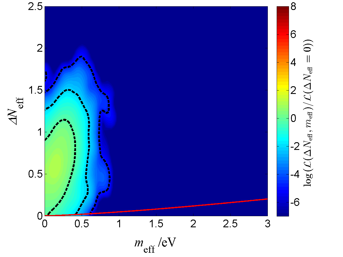
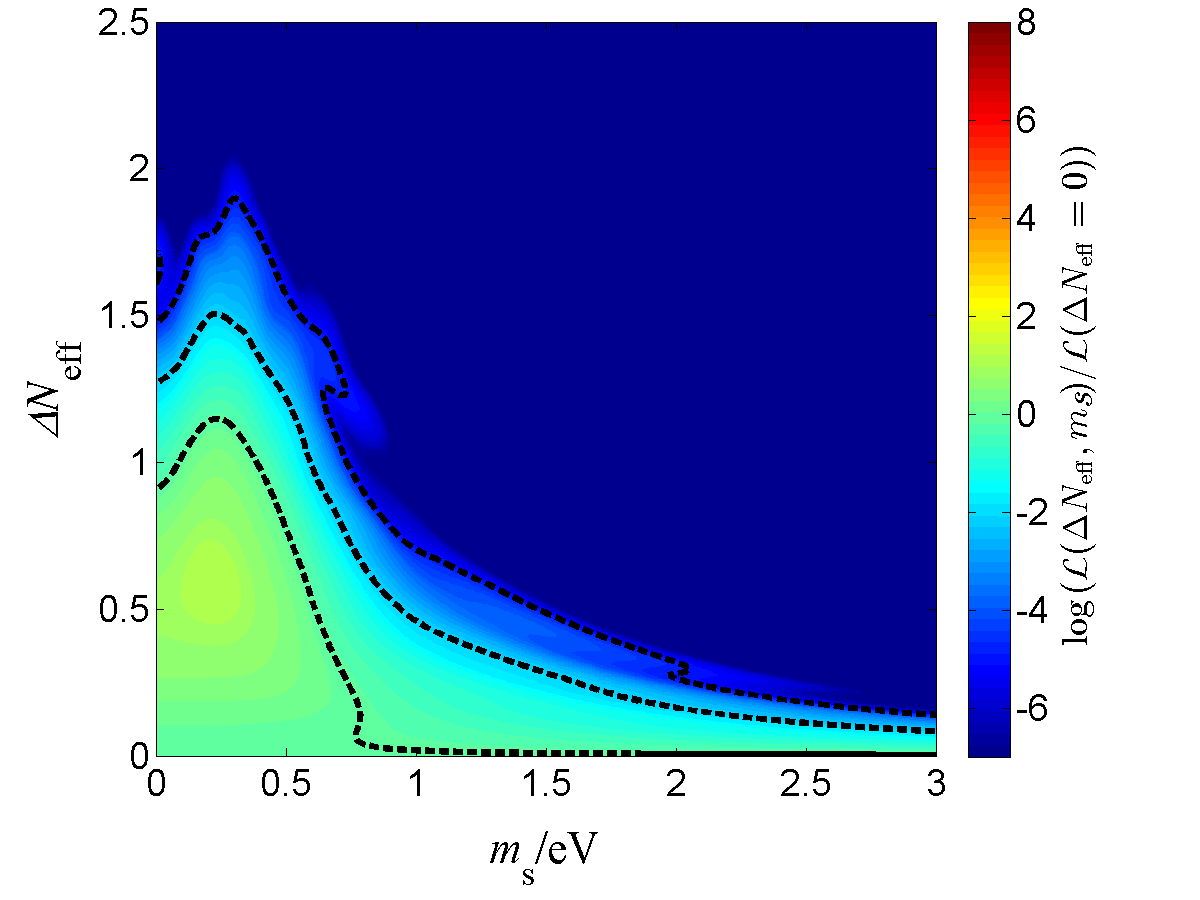
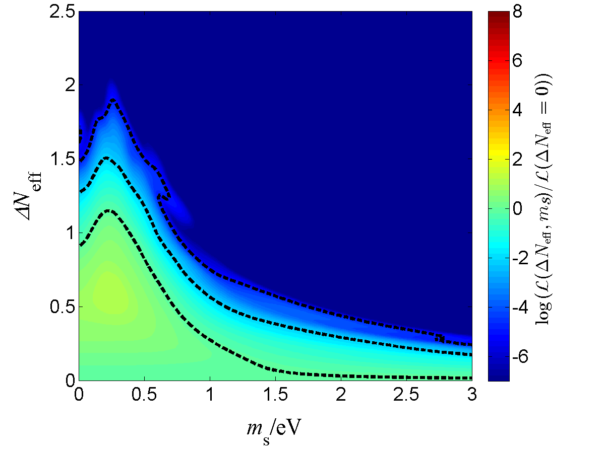
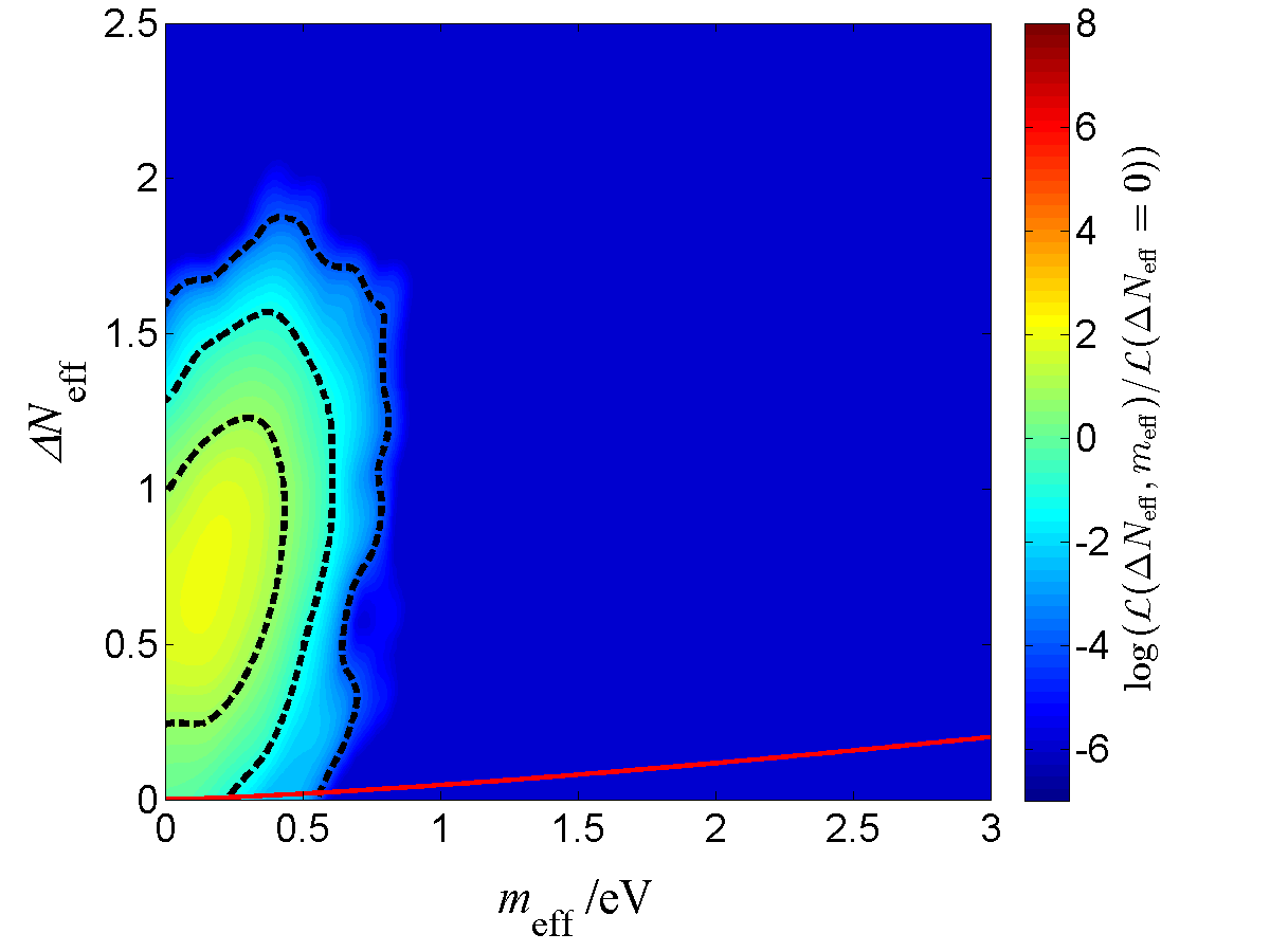
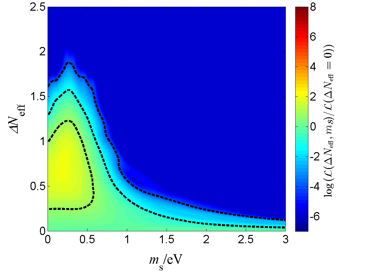
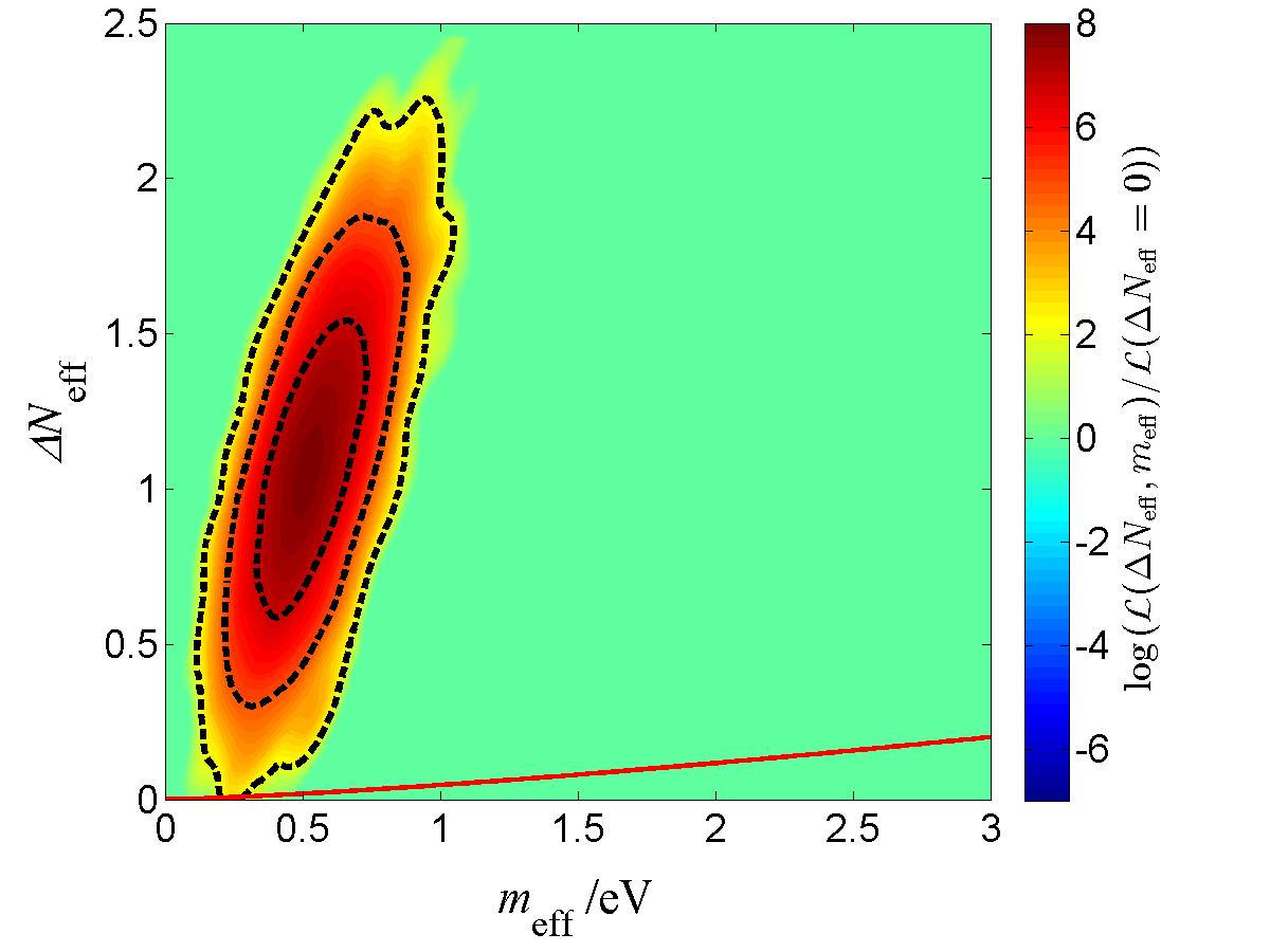
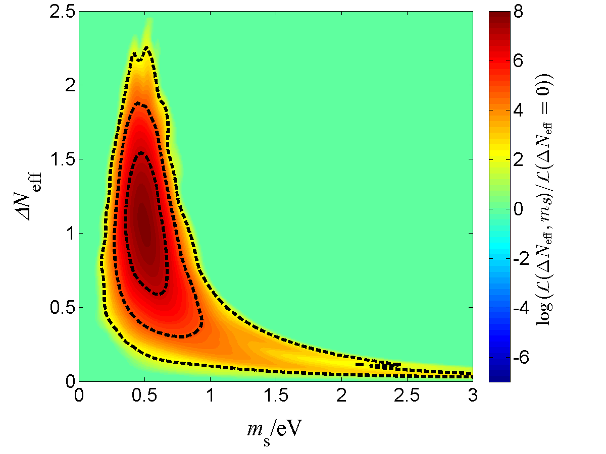
The results of our analysis for the three data set combinations described in Sec. 3.1 are shown in Figs. 1 and  2.

In the the upper left panel of Fig. 1 and in the left panels of Fig. 2 we plot the contours of the marginal likelihood $\mathcal{L}(N_{\rm eff},m_{\rm eff})$ normalized to the value of $\mathcal{L}(\Delta N_{\rm eff}=0)$ (which does not depend on $m_{\rm eff}$) . The red contour delimits the regions for which $m_{s}$ in Eq. (14) exceeds 10 eV for which the sterile states becomes indistinguishable from cold or warm dark matter Ade:2013lta and hence for values of the parameters below the curve, the marginal likelihood is not evaluated. Black dashed contours are those of $-2\log(\mathcal{L}/\mathcal{L}^{\rm max})<2.30,6.18,11.83$, nominally corresponding to the $1\sigma$, $2\sigma$, and $3\sigma$ levels in two dimensions.

In the upper right panel of Fig. 1 and the right panels of Fig. 2 we show the contours of the marginal likelihood of $(N_{\rm eff},m_{s})$ for the thermally distributed sterile neutrinos while in the lower left panel of Fig. 1 we show the corresponding marginal likelihood in the DW scenario. We see that for both DW and thermal $\nu_{s}$ scenarios, $m_{s}$ becomes increasingly large for decreasing $\Delta N_{\text{\rm eff}}$, hence the distinctive appearance of large “flat” regions and weak constraints on $m_{\text{\rm s}}$ for small $\Delta N_{\text{\rm eff}}$. Also as seen in Fig. 1 the results for the DW and the thermal $\nu_{s}$ scenarios are qualitatively very similar. Only, since for fixed $m_{\rm eff}$ and $\Delta N_{\text{\rm eff}}$, $m_{s}^{\rm DW}=m_{s}^{\rm TH}\Delta N_{\text{\rm eff}}^{-1/4}$, for $\Delta N_{\text{\rm eff}}\leq 1$ the likelihood contours in the DW scenario are shifted to slightly larger masses in an amount which decreases as $\Delta N_{\text{\rm eff}}$ increases.

The impact of BICEP2 data can be seen by comparing the upper panels in Fig. 1 and  Fig. 2. The addition of BICEP2 data gives a preference for large values of the tensor-to-scalar ratio $r$ and, due to its correlation with $\Delta N_{\text{\rm eff}}$, and therefore leads to the the shift to slightly larger values of $\Delta N_{\text{\rm eff}}$ observed in upper panels in  Fig. 2. Since $r$ is now better constrained, also the preferred region becomes slightly smaller.

The effects of adding HST+PlaSZ in the analysis are displayed in the lower panels in Fig. 2 where we see a shift to larger values of both $\Delta N_{\text{\rm eff}}$ and $m_{\text{\rm eff}}$. This is so because the constraints on $\sigma_{8}$ of the PlaSZ measurement, which are in tension with the other experiments within this model, can be somewhat alleviated by an increase in $m_{\text{\rm eff}}$, while the inclusion of HST yields an increase $\Delta N_{\text{\rm eff}}$.

All these results are in qualitative agreement with those in the analyses in Refs. Archidiacono:2014apa ; Dvorkin:2014lea ; Zhang:2014dxk ; Zhang:2014nta ; Wu:2014qxa ; Leistedt:2014sia ; Giusarma:2014zza . However we notice that by showing the marginal likelihood we are explicitly not assigning any priors to the sterile parameters. This is an advantage in the absence of a physical motivation for them, especially $m_{\text{\rm s}}$, since the data at hand is expected to leave a large prior dependence. For example, if one used a prior on $m_{\text{\rm s}}$ which is uniform in $\log m_{\text{\rm s}}$ instead of in $m_{\text{\rm s}}$, as in general the likelihood is non-negligible for a vanishing sterile mass, the derived Bayesian constraints on $m_{\text{\rm eff}}$ and $\Delta N_{\text{\rm eff}}$ would be very different. In principle one could embark on an extensive prior sensitivity analysis, but in this work we will instead focus on analyses for which the results have little or no prior dependence.

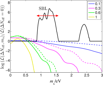
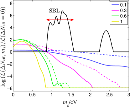
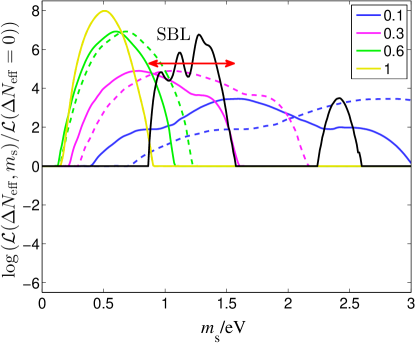
Finally, in order to better illustrate how the constraints depend on the sterile mass we plot in Fig. 3, the slices of the marginal likelihood as a function of $m_{s}$ for fixed $\Delta N_{\rm eff}$. Also shown in the figure is the marginal likelihood for the SBL analysis in the 3+1 scenario (marginalized with respect to the lighter neutrino masses and all mixings) as given in Fig.1 in Ref. Kristiansen:2013mza .

CMB+BAO
	Thermal $\nu_{s}$
Dodelson-Widrow scenario

Figure 1: Marginal likelihood of $(m_{\rm eff},\Delta N_{\rm eff})$ (upper right panel) and of $(m_{s},\Delta N_{\rm eff})$ for thermally distributed $\nu_{s}$ (upper left panel) and for the for DW scenario (lower panel) for the CMB+BAO cosmological data set (SET 1). Black dashed contours are those of $-2\log(\mathcal{L}/\mathcal{L}^{\rm max})<C$, which would correspond to nominal 1,2,3 sigma levels. The red line denotes the region for which $m_{s}=10$ eV for thermal $\nu_{s}$.

CMB+BAO+BICEP2
	Thermal $\nu_{s}$
CMB+BAO+BICEP2+HST+PlaSZ

Figure 2: Same two upper panels in Fig. 1, but for CMB+BAO+BICEP2 cosmological data (SET 2, upper panels), and CMB+BAO+BICEP2+HST+PlaSZ cosmological data (SET 3, lower panels).

CMB+BAO	CMB+BAO+BICEP2
CMB+BAO+BICEP2+HST+PlaSZ

Figure 3: Marginal likelihoods as function of $m_{s}$ for fixed $\Delta N_{\rm eff}$ ($\Delta N_{\rm eff}=0.1,0.3,0.6,1$) and for thermal $\nu_{s}$ (solid lines) and for the DW scenario (dashed lines). We show the results for the three cosmological data sets used as labeled in the figure. In all panels we also include the marginal likelihood for the SBL analysis in the 3+1 scenario (marginalized with respect to the lighter neutrino masses and all mixings) as given in Fig.1 in Ref. Kristiansen:2013mza . We denote by the red arrow the width and height of the box used to define “box SBL likelihood” (see text for details).

4 Test on sterile neutrinos models

In this section we perform the statistical tests on the 3+1 scenarios invoked to explain the SBL anomalies using the results of the cosmological analysis presented in the previous section. In doing so we are going to assume that the contribution of the sterile neutrino to the cosmological observables is independent of the active-sterile neutrino mixing (see discussion around Eq. (12)). Under this assumption our tests will require the marginalized likelihood of the sterile neutrino mass $m_{s}$ obtained from the analysis of the SBL anomalies in the 3+1 scenario (marginalized with respect to all other oscillation parameters in the scenario), and the marginalized likelihoods of $(m_{s},\Delta N_{\rm eff})$ from the cosmological analysis previously presented.

Concerning the SBL likelihood, we consider two different functions that can be interpreted as the two limiting cases. In the first, we consider the precise SBL likelihood as given in Fig. 1 in Ref. Kristiansen:2013mza which we reproduce in Fig. 3 (in this case below roughly seven log-units from the maximum value, we set the SBL likelihood to a constant value). We label this case in the following as “full SBL likelihood”. In the second case, we approximate the SBL likelihood as a top-hat shaped likelihood which is constant and non-zero between 0.86 eV and 1.57 eV and zero otherwise (which we illustrate by the arrow in Fig. 3). This is what we label in the following as “box SBL likelihood”.

4.1 Sterile neutrinos vs none

The first question we want to address is whether the current data shows evidence of the existence of sterile neutrinos, and how strong this evidence is. Generically in Bayesian analyses this takes the form of model comparison between a model without sterile neutrinos and a model with sterile neutrinos using some posterior odds, Eq. (5). There are several ways to go about answering this question. In here we are interested in testing what cosmology has to say on this comparison for the sterile models invoked to explain the SBL anomalies. This is, in this case the first model $H_{0}$ is defined as a model with no sterile neutrino, which implies a cosmological model with $\Delta N_{\text{\rm eff}}=0$. And the other model, $H_{1}$ is taken to include one sterile neutrino of mass $m_{\rm s}$ as required to accommodate the SBL anomalies and which contributes to relativistic energy density in the early Universe as some fix $\Delta N_{\text{\rm eff}}$.

In this case we can define a posterior odds as:

$$\mathcal{O} = \frac{\Pr(D_{\text{c}}|D_{\text{SBL}},H_{1})}{\Pr(D_{\text{c}}|D_{\text{SBL}},H_{0})}\frac{\Pr(H_{1}|D_{\text{SBL}})}{\Pr(H_{0}|D_{\text{SBL}})}=$$

$$= \frac{\Pr(D_{\text{c}}|D_{\text{SBL}},H_{1})}{\Pr(D_{\text{c}}|D_{\text{SBL}},H_{0})}\frac{\Pr(D_{\text{SBL}}|H_{1})}{\Pr(D_{\text{SBL}}|H_{0})}\frac{\Pr(H_{1})}{\Pr(H_{0})}$$

$$\equiv \mathcal{B}^{\text{upd}}_{10}\mathcal{B}^{\rm SBL}_{10}\frac{\Pr(H_{1})}{\Pr(H_{0})}\,,$$

with

$$\mathcal{B}^{\rm SBL}_{10} \equiv \frac{\Pr(D_{\text{SBL}}|H_{1})}{\Pr(D_{\text{SBL}}|H_{0})}$$ (18)

and

$$\mathcal{B}^{\text{upd}}_{10} \equiv \frac{\Pr(D_{\text{c}}|D_{\text{SBL}},H_{1})}{\Pr(D_{\text{c}}|D_{\text{SBL}},H_{0})}=\frac{\Pr(D_{\text{c}}|D_{\text{SBL}},H_{1})}{\Pr(D_{\text{c}}|H_{0})}=\frac{\Pr(D_{\text{c}},D_{\text{SBL}}|H_{1})}{\Pr(D_{\text{c}}|H_{0})\Pr(D_{\text{SBL}}|H_{1})}\,,$$ (19)

where in the last line we have used that SBL is not sensitive to any parameters effecting cosmology once we assume that there are no sterile neutrinos and hence $D_{\text{SBL}}$ and $D_{\text{c}}$ are independent under $H_{0}$. The quantity $\mathcal{B}^{\text{upd}}_{10}$ quantifies how much better the prediction of cosmological data assuming sterile neutrino and SBL data is than the prediction assuming no sterile neutrinos.

Now, the model $H_{1}$ is inherently more complex than $H_{0}$ since it contains additional parameters (sterile mass and mixings), and this is as usual compensated for in a Bayesian analysis. In the first row of Eq. (4.1) this is contained in the last factor of $\Pr(H_{1}|D_{\text{SBL}})/\Pr(H_{0}|D_{\text{SBL}})=\mathcal{B}^{\rm SBL}_{10}\frac{\Pr(H_{1})}{\Pr(H_{0})}$. Now, the best-fit of the SBL data is significantly better if you have a sterile neutrino, but because of the added complexity it might not be totally unreasonable to have $\Pr(H_{1}|D_{\text{SBL}})/\Pr(H_{0}|D_{\text{SBL}})=\mathcal{O}(1)$.

In any case, it is the first factor in Eq. (4.1) the factor by which the cosmological data have updated the SBL-only posterior odds to the final SBL+cosmology odds and which we will be using in our quantification. Furthermore, under the additional assumption that $\Delta N_{\text{\rm eff}}$ is unconstrained by SBL data, $\Pr(D_{\text{SBL}}|H_{1})$ does not depend on $\Delta N_{\text{\rm eff}}$, and hence $\mathcal{B}_{10}^{\text{upd}}$ is in fact simply proportional to the combined marginal likelihood of $\Delta N_{\text{\rm eff}}$, normalized such that $\mathcal{B}_{10}^{\text{upd}}=1$ for $\Delta N_{\text{\rm eff}}=0$.

Before discussing the results, let us mention that here, as in any Bayesian analysis, the results are in principle always prior dependent, and we should consider how large this dependence is in practice. First, as discussed in Sec. 3, the marginal likelihood depends on the priors on the cosmological nuisance parameters, but this dependence is expected to be small (except possibly for $r$). More significantly, there is the dependence of the total Bayes factor and odds on the prior on $m_{s}$, even when it is well constrained by the combined data set. However the value of $\mathcal{B}_{10}^{\text{upd}}$ does not strongly depend on the the shape of the prior nor its upper limit. This is so because the well-constraining SBL data is used to update the prior to a posterior (which is rather insensitive to the prior) which is then used to analyze the cosmological data. We use a uniform prior between $0$ and $10\;\text{eV}$ as the nominal upper limit, since, as described in Ref. Ade:2013lta , this roughly defines the region where (for the CMB) the particles are distinct from cold or warm dark matter.

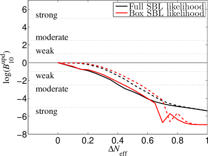
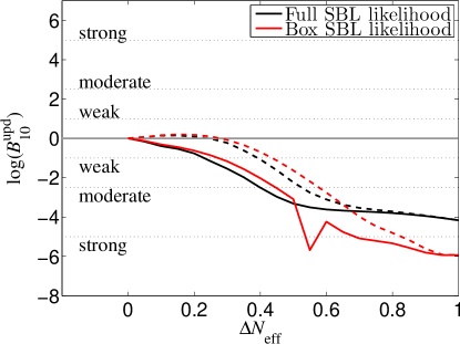
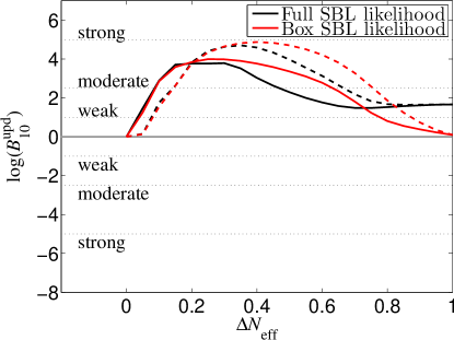
The results are shown in the left panel of Fig. 4. We see that for the CMB+BAO and CMB+BAO+BICEP2 data sets, $\mathcal{B}_{10}^{\text{upd}}$ decreases quite steadily with $\Delta N_{\text{\rm eff}}$. These cosmological data hence disfavour models with sterile neutrinos required to explain the SBL anomalies over the model without sterile neutrinos independently of how much the contribution of the sterile neutrino to the energy density is suppressed with respect to the fully thermalized expectation. We also see that the addition of the BICEP2 data has a small impact on these conclusions.

For the CMB+BAO+BICEP2+HST+PlaSZ data set, there is, on the contrary, a significant peak for intermediate values of $\Delta N_{\text{\rm eff}}$. The $\Lambda$CDM$+r$ model is significantly disfavoured by this combination of cosmological data, while increasing $\Delta N_{\text{\rm eff}}$ increases the cosmological likelihood for SBL-compatible masses. However, further increasing $\Delta N_{\text{\rm eff}}$, cosmology requires a too small mass, so the $\mathcal{B}_{10}^{\text{upd}}$ decrease again. Notice also that in fact the $\Lambda$CDM$+r$ is so disfavored that it is in the region where the (too large) constant extrapolation is used. Hence, the exact $\mathcal{B}_{10}^{\text{upd}}$ is expected to be even larger.

CMB+BAO
CMB+BAO+BICEP2
CMB+BAO+BICEP2+HST+PlaSZ

Figure 4: Left panels:Logarithm of the Bayes factor $\mathcal{B}_{10}^{\text{upd}}$ as a function of $\Delta N_{\rm eff}$. Right panels: Consistency of mass constraints. In all panels the results are shown for thermal $\nu_{s}$ (solid lines) and for the DW scenario (dashed lines) and for the SBL full (black) and Box likelihood (red). We show the results for the three cosmological data sets considered: CMB+BAO (upper row), CMB+BAO+BICEP2 (middle row), CMB+BAO+BICEP2+HST+PlaSZ (lower row).

4.2 Consistency of parameter constraints

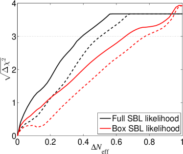
In addition to comparing the models with and without sterile neutrinos we now address the question of the consistency of the parameter constraints from the different data sets within the 3+1 model. A Bayesian test was formulated in Marshall:2004zd , in which a model where both data sets are fitted by the same physical parameters is compared with a model in which each data set uses their own parameters. However, as is often the case in model comparison, the result can depend crucially on the prior on the parameters, in our case $m_{s}$ in particular. Since we cannot motivate using a specific shape or limits on the prior, we instead use the corresponding $\chi^{2}$-test (these were also compared in Marshall:2004zd ). Although not rigorous as the Bayesian test, it has the clear advantage that it is prior-independent.

In particular, if we want to test how inconsistent the constraints on the sterile mass from the different data sets are once a certain $\Delta N_{\text{\rm eff}}$ is assumed, i.e., without considering how favoured or disfavoured that $\Delta N_{\text{\rm eff}}$ is by the cosmological data, we should evaluate

$$\Delta\chi^{2}(\Delta N_{\text{\rm eff}})=\hat{\chi}^{2}_{\rm comb}(\Delta N_{\text{\rm eff}})-\hat{\chi}^{2}_{\rm SBL}-\hat{\chi}^{2}_{\rm cosmo}(\Delta N_{\text{\rm eff}})\;,,$$ (20)

where the hat denotes the value at the best fit i.e., optimized over $m_{s}$ ($\chi^{2}_{\rm SBL}$ does not depend on $\Delta N_{\text{\rm eff}}$).

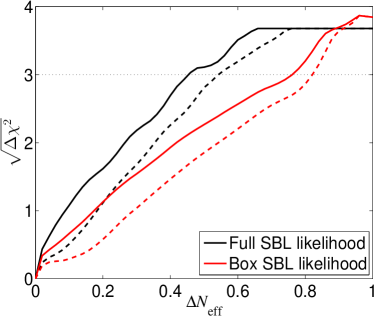
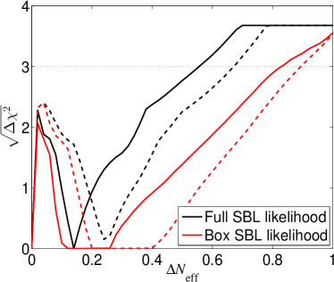
The results of this test are shown on the right-hand side of Fig. 4. As expected, the results for CMB+BAO and CMB+BAO+BICEP2 are quite similar and show an steady increase of the inconsistency with $\Delta N_{\text{\rm eff}}$. Also comparing the DW and thermal scenarios, we see that in general to obtain the same $\Delta\chi^{2}$ larger values of $\Delta N_{\text{\rm eff}}$ are required in the DW scenario. This is so because, as explained before, in the DW scenario the preferred masses are shifted to larger values by an amount which increases as $\Delta N_{\text{\rm eff}}<1$ decreases. As for the results for the box and full SBL likelihoods, we notice that, typically, using the full SBL likelihood gives a larger inconsistency. This is because the box likelihood is constant over a wide range of $m_{s}$, and over this wide range the cosmological likelihood typically varies significantly. The combined $\chi^{2}$ can then easily be reduced by finding the best fit within this range.

For the CMB+BAO+BICEP2+HST+PlaSZ combination, one observes in each curve a peak for small value of $\Delta N_{\text{\rm eff}}$, although it does not reach the level of $2.5\sigma$. These peaks are due to the fact that (cf. Fig. 2) cosmology prefers large physical masses, too large to fit the SBL data. As $\Delta N_{\text{\rm eff}}$ increases, the mass constraints become compatible, but as $\Delta N_{\text{\rm eff}}$ continues to decrease, cosmology requires the masses to be smaller than those which can fit the SBL data and the inconsistency increases.

Again, we stress that this consistency test is in principle not affected by how favoured or disfavoured the considered value of $\Delta N_{\text{\rm eff}}$ is, but instead consider that value to be “true”, and then test the compatibility of the constraints on the mass. For example, comparing the left and right panels in the last raw of Fig. 4 we see that for the CMB+BAO+BICEP2+HST+PlaSZ data set, even though from the right panel we read that the mass ranges required for cosmology and SBL become highly incompatible for $\Delta N_{\text{\rm eff}}$ close to one, from the left hand side we see that these large values of $\Delta N_{\text{\rm eff}}$ are not particularly disfavoured compared to small $\Delta N_{\text{\rm eff}}$, for which the mass constraints are compatible. So what we see is that large $\Delta N_{\text{\rm eff}}$ is disfavoured because the sterile mass required by SBL and cosmology are incompatible and small $\Delta N_{\text{\rm eff}}$ is disfavoured because it is so in the cosmological (and consequently in the combined) analysis. So small and large $\Delta N_{\text{\rm eff}}$ have comparable Bayes factors, but this is only because they are both disfavoured.

5 Summary

In this paper we have revisited the question of the information which cosmology provides on the scenarios with O(eV) mass sterile neutrinos invoked to explain the SBL anomalies (Eq. (1)) using Bayesian statistical tests and study how the results depend on the inclusion of the recently CMB polarization results of BICEP2 and on the inclusion of local measurements which show some tension with the Planck and LSS-BAO results when analyzed in the framework of the $\Lambda$CDM scenario.

In order to do so we have first performed an analysis of three characteristic sets of cosmological data in $\Lambda$CDM$+r+\nu_{s}$ cosmologies as described in Sec. 3. The result of our analysis is presented in Figs. 1 and  2 in the form of marginalized cosmological likelihoods in terms of the two relevant parameters, the sterile neutrino mass $m_{s}$ and its contribution to the energy density of the early Universe $\Delta N_{\text{\rm eff}}$. The results clearly indicate that as long as the HST and SZ cluster data from Planck are not included, cosmological data favours the sterile neutrino mass $m_{s}$ clearly well below $eV$ unless its contribution to the energy density is suppressed with respect to the expected from a fully thermalized sterile neutrino. The inclusion of the BICEP2 data does not substantially affect this conclusion. Conversely including these HST and SZ cluster data higher sterile masses become favoured.

With these results, we have performed in Sec. 4 two statistical test on their (in)compatibility with the corresponding likelihood derived from the analysis of the SBL results as given in Ref. Kristiansen:2013mza . In the first test we have asked ourselves whether cosmology favours or disfavours the 3+1 sterile models which explain the SBL results over a model without sterile neutrinos. In order to do so we have constructed the Bayes factor defined in Eq. (19) which gives the factor by which the cosmological data updates the SBL-only posterior odds of the 3+1 vs 3+0 model to the final SBL+cosmology odds and we have studied its behaviour as a function of $\Delta N_{\text{\rm eff}}$. The results of this test, shown in Fig. 4 implies that as long as the HST and SZ cluster data from Plank is not included, the cosmological analysis disfavour the 3+1 model with respect to 3+0. The inclusion of these cosmological data however favours the 3+1 model for an intermediate range of $\Delta N_{\text{\rm eff}}$. We summarize in Tab. 3 the ranges of $\Delta N_{\text{\rm eff}}$ for which we find the evidence against or in favour of the 3+1 model compared to the model with only the 3 active neutrinos to be weak, moderate or strong from these analyses.

Evidence	Scenario	SET 1	SET 2	SET 3
	/SBL Likel	3+1 Disfavoured	3+1 Disfavoured	3+1 Favoured
	TH/FULL	$[0.22,0.40]$	$[0.23,0.40]$	$[0.03,0.08]$ $\oplus$	$\geq 0.47$
Weak	TH/BOX	$[0.25,0.44]$	$[0.27,0.45]$	$[0.04,0.09]$ $\oplus$	$[0.63,0.78]$
	DW/FULL	$[0.35,0.51]$	$[0.39,0.52]$	$[0.08,0.14]$ $\oplus$	$\geq 0.67$
	DW/BOX	$[0.38,0.55]$	$[0.44,0.58]$	$[0.08,0.14]$ $\oplus$	$[0.76,0.87]$
	TH/FULL	$[0.40,0.86]$	$\geq 0.40$	$[0.08,0.47]$
Moderate	TH/BOX	$[0.44,0.66]$	$[0.45,0.53]$  $\oplus$  $[0.57,0.68]$	$[0.09,0.63]$
	DW/FULL	$[0.51,0.86]$	$\geq 0.52$	$[0.14,0.67]$
	DW/BOX	$[0.55,0.72]$	$[0.58,0.83]$	$[0.14,0.76]$
	TH/FULL	$\geq 0.86$	–	–
Strong	TH/BOX	$\geq 0.66$	$[0.53,0.57]$ $\oplus$  $\geq 0.68$	–
	DW/FULL	$\geq 0.86$	–	–
	DW/BOX	$\geq 0.72$	$\geq 0.83$	–

Table 3: Ranges of $\Delta N_{\text{\rm eff}}$ for which we find the evidence against or in favour of the 3+1 model compared to the model with only the 3 active neutrinos to be weak, moderate or strong.

The second test performed deals with the (in)compatibility of the sterile mass constraints as required to describe SBL and cosmology. For this we have evaluated the $\Delta\chi^{2}$ defined in Eq. (20) which we plot in the right panels in Fig. 4. Altogether we read that this test yields inconsistency on the $m_{s}$ required by cosmology and SBL larger than $3\sigma$ for

$$\Delta N_{\text{\rm eff}}\geq 0.45\,(0.54)\,[0.76]\,\left([0.82]\right)\;\;{\rm For\,CMB+BAO}\>,$$

$$\Delta N_{\text{\rm eff}}\geq 0.39\,(0.50)\,[0.65]\,\left([0.77]\right)\;\;{\rm For\,CMB+BAO+BICEP2}\;,$$ (21)

$$\Delta N_{\text{\rm eff}}\geq 0.56\,(0.67)\,[0.83]\,\left([0.89]\right)\;\;{\rm For\,CMB+BAO+BICEP2+HST+PlaSZ}\;,$$

for thermal (WP) $\nu_{s}$ scenario for the full [box] SBL likelihood.

In summary, we find that the analysis of cosmological results from temperature and polarization data on the CMB as well as from the BAO measurements from LSS data disfavours the 3+1 sterile models introduced to explain the SBL anomalies over the scenario without sterile neutrinos, and also that their allowed/required ranges of $m_{s}$ are incompatible. This is so even if new physics is involved so that the contribution of the sterile neutrino to the energy density of the Universe (and therefore to the cosmological observables) is suppressed with respect to that of the fully thermalized case resulting from its mixing with the active neutrinos. When the local measurement of the $H_{0}$ by the Hubble Space Telescope, and the cluster SZ cluster data from the Planck mission is included, compatibility can be found between cosmological and SBL data, but still requires a substantial suppression of the $\nu_{s}$ contribution to $\rho_{R}$.

References

- (1) B. Pontecorvo, Neutrino experiments and the problem of conservation of leptonic charge, Sov. Phys. JETP 26 (1968) 984–988
- (2) V. Gribov and B. Pontecorvo, Neutrino astronomy and lepton charge, Phys. Lett. B28 (1969) 493
- (3) M. Gonzalez-Garcia and M. Maltoni, Phenomenology with Massive Neutrinos, Phys.Rept. 460 (2008) 1–129, [arXiv:0704.1800]
- (4) M. Gonzalez-Garcia, M. Maltoni, J. Salvado, and T. Schwetz, Global fit to three neutrino mixing: critical look at present precision, JHEP 1212 (2012) 123, [arXiv:1209.3023]
- (5) K. Abazajian, M. Acero, S. Agarwalla, A. Aguilar-Arevalo, C. Albright, et. al., Light Sterile Neutrinos: A White Paper, arXiv:1204.5379
- (6) A. Aguilar et. al., Evidence for neutrino oscillations from the observation of appearance in a beam, Phys. Rev. D64 (2001) 112007, [hep-ex/0104049]
- (7) A. A. Aguilar-Arevalo et. al., Event excess in the MiniBooNE search for oscillations, Phys. Rev. Lett. 105 (2010) 181801, [arXiv:1007.1150]
- (8) A. Aguilar-Arevalo et. al., Improved Search for Oscillations in the MiniBooNE Experiment, Phys.Rev.Lett. 110 (2013), no. 16 161801, [arXiv:1207.4809]
- (9) G. Mention, M. Fechner, T. Lasserre, T. Mueller, D. Lhuillier, et. al., The Reactor Antineutrino Anomaly, Phys.Rev. D83 (2011) 073006, [arXiv:1101.2755]
- (10) T. Mueller, D. Lhuillier, M. Fallot, A. Letourneau, S. Cormon, et. al., Improved Predictions of Reactor Antineutrino Spectra, Phys.Rev. C83 (2011) 054615, [arXiv:1101.2663]
- (11) P. Huber, On the determination of anti-neutrino spectra from nuclear reactors, Phys.Rev. C84 (2011) 024617, [arXiv:1106.0687]
- (12) C. Giunti and M. Laveder, Statistical Significance of the Gallium Anomaly, Phys.Rev. C83 (2011) 065504, [arXiv:1006.3244]
- (13) C. Giunti, M. Laveder, Y. Li, Q. Liu, and H. Long, Update of Short-Baseline Electron Neutrino and Antineutrino Disappearance, Phys.Rev. D86 (2012) 113014, [arXiv:1210.5715]
- (14) M. A. Acero, C. Giunti, and M. Laveder, Limits on nu(e) and anti-nu(e) disappearance from Gallium and reactor experiments, Phys.Rev. D78 (2008) 073009, [arXiv:0711.4222]
- (15) J. Kopp, M. Maltoni, and T. Schwetz, Are there sterile neutrinos at the eV scale?, Phys.Rev.Lett. 107 (2011) 091801, [arXiv:1103.4570]
- (16) C. Giunti and M. Laveder, 3+1 and 3+2 Sterile Neutrino Fits, Phys.Rev. D84 (2011) 073008, [arXiv:1107.1452]
- (17) C. Giunti and M. Laveder, Status of 3+1 Neutrino Mixing, Phys.Rev. D84 (2011) 093006, [arXiv:1109.4033]
- (18) C. Giunti and M. Laveder, Implications of 3+1 Short-Baseline Neutrino Oscillations, Phys.Lett. B706 (2011) 200–207, [arXiv:1111.1069]
- (19) A. Donini, P. Hernandez, J. Lopez-Pavon, M. Maltoni, and T. Schwetz, The minimal 3+2 neutrino model versus oscillation anomalies, JHEP 1207 (2012) 161, [arXiv:1205.5230]
- (20) J. Conrad, C. Ignarra, G. Karagiorgi, M. Shaevitz, and J. Spitz, Sterile Neutrino Fits to Short Baseline Neutrino Oscillation Measurements, Adv.High Energy Phys. 2013 (2013) 163897, [arXiv:1207.4765]
- (21) C. Giunti, M. Laveder, Y. Li, and H. Long, Pragmatic View of Short-Baseline Neutrino Oscillations, Phys.Rev. D88 (2013) 073008, [arXiv:1308.5288]
- (22) G. Karagiorgi, M. Shaevitz, and J. Conrad, Confronting the short-baseline oscillation anomalies with a single sterile neutrino and non-standard matter effects, arXiv:1202.1024
- (23) J. Kopp, P. A. N. Machado, M. Maltoni, and T. Schwetz, Sterile neutrino oscillations: The global picture, arXiv:1303.3011
- (24) K. Nakamura et. al., Review of particle physics, J. Phys. G37 (2010) 075021
- (25) G. Mangano, G. Miele, S. Pastor, T. Pinto, O. Pisanti, et. al., Relic neutrino decoupling including flavor oscillations, Nucl.Phys. B729 (2005) 221–234, [hep-ph/0506164]
- (26) N. Saviano, A. Mirizzi, O. Pisanti, P. D. Serpico, G. Mangano, et. al., Multi-momentum and multi-flavour active-sterile neutrino oscillations in the early universe: role of neutrino asymmetries and effects on nucleosynthesis, Phys.Rev. D87 (2013) 073006, [arXiv:1302.1200]
- (27) A. Mirizzi, G. Mangano, N. Saviano, E. Borriello, C. Giunti, et. al., The strongest bounds on active-sterile neutrino mixing after Planck data, Phys.Lett. B726 (2013) 8–14, [arXiv:1303.5368]
- (28) M. Gonzalez-Garcia, M. Maltoni, and J. Salvado, Robust Cosmological Bounds on Neutrinos and their Combination with Oscillation Results, JHEP 1008 (2010) 117, [arXiv:1006.3795]
- (29) M. A. Acero and J. Lesgourgues, Cosmological constraints on a light non-thermal sterile neutrino, Phys.Rev. D79 (2009) 045026, [arXiv:0812.2249]
- (30) J. Hamann, S. Hannestad, G. G. Raffelt, I. Tamborra, and Y. Y. Wong, Cosmology seeking friendship with sterile neutrinos, Phys.Rev.Lett. 105 (2010) 181301, [arXiv:1006.5276]
- (31) E. Giusarma, M. Archidiacono, R. de Putter, A. Melchiorri, and O. Mena, Sterile neutrino models and nonminimal cosmologies, Phys.Rev. D85 (2012) 083522, [arXiv:1112.4661]
- (32) M. Archidiacono, E. Calabrese, and A. Melchiorri, The Case for Dark Radiation, arXiv:1109.2767
- (33) M. Archidiacono, N. Fornengo, C. Giunti, and A. Melchiorri, Testing 3+1 and 3+2 neutrino mass models with cosmology and short baseline experiments, Phys.Rev. D86 (2012) 065028, [arXiv:1207.6515]
- (34) M. Gonzalez-Garcia, V. Niro, and J. Salvado, Dark Radiation and Decaying Matter, JHEP 1304 (2013) 052, [arXiv:1212.1472]
- (35) P. Di Bari, S. F. King, and A. Merle, Dark Radiation or Warm Dark Matter from long lived particle decays in the light of Planck, Phys.Lett. B724 (2013) 77–83, [arXiv:1303.6267]
- (36) J. Hasenkamp and J. Kersten, Dark radiation from particle decay: cosmological constraints and opportunities, JCAP 1308 (2013) 024, [arXiv:1212.4160]
- (37) P. Graf and F. D. Steffen, Dark radiation and dark matter in supersymmetric axion models with high reheating temperature, JCAP 1312 (2013) 047, [arXiv:1302.2143]
- (38) P. Ade et. al., Planck 2013 results. XVI. Cosmological parameters, arXiv:1303.5076
- (39) S. Das, T. Louis, M. R. Nolta, G. E. Addison, E. S. Battistelli, et. al., The Atacama Cosmology Telescope: Temperature and Gravitational Lensing Power Spectrum Measurements from Three Seasons of Data, arXiv:1301.1037
- (40) R. Keisler, C. Reichardt, K. Aird, B. Benson, L. Bleem, et. al., A Measurement of the Damping Tail of the Cosmic Microwave Background Power Spectrum with the South Pole Telescope, Astrophys.J. 743 (2011) 28, [arXiv:1105.3182]
- (41) C. Reichardt, L. Shaw, O. Zahn, K. Aird, B. Benson, et. al., A measurement of secondary cosmic microwave background anisotropies with two years of South Pole Telescope observations, Astrophys.J. 755 (2012) 70, [arXiv:1111.0932]
- (42) P. Ade et. al., Detection of B-Mode Polarization at Degree Angular Scales by BICEP2, Phys.Rev.Lett. 112 (2014) 241101, [arXiv:1403.3985]
- (43) L. Verde, S. M. Feeney, D. J. Mortlock, and H. V. Peiris, (Lack of) Cosmological evidence for dark radiation after Planck, JCAP 1309 (2013) 013, [arXiv:1307.2904]
- (44) M. Archidiacono, N. Fornengo, S. Gariazzo, C. Giunti, S. Hannestad, et. al., Light sterile neutrinos after BICEP-2, JCAP 1406 (2014) 031, [arXiv:1404.1794]
- (45) C. Dvorkin, M. Wyman, D. H. Rudd, and W. Hu, Neutrinos help reconcile Planck measurements with both Early and Local Universe, arXiv:1403.8049
- (46) J.-F. Zhang, Y.-H. Li, and X. Zhang, Sterile neutrinos help reconcile the observational results of primordial gravitational waves from Planck and BICEP2, arXiv:1403.7028
- (47) J.-F. Zhang, Y.-H. Li, and X. Zhang, Cosmological constraints on neutrinos after BICEP2, arXiv:1404.3598
- (48) F. Wu, Y. Li, Y. Lu, and X. Chen, Cosmological parameter fittings with the BICEP2 data, arXiv:1403.6462
- (49) B. Leistedt, H. V. Peiris, and L. Verde, No new cosmological concordance with massive sterile neutrinos, arXiv:1404.5950
- (50) E. Giusarma, E. Di Valentino, M. Lattanzi, A. Melchiorri, and O. Mena, Relic Neutrinos, thermal axions and cosmology in early 2014, arXiv:1403.4852
- (51) J. Hamann, S. Hannestad, G. G. Raffelt, and Y. Y. Wong, Sterile neutrinos with eV masses in cosmology: How disfavoured exactly?, JCAP 1109 (2011) 034, [arXiv:1108.4136]
- (52) J. R. Kristiansen, . Elgarøy, C. Giunti, and M. Laveder, Cosmology with sterile neutrino masses from oscillation experiments, arXiv:1303.4654
- (53) M. Archidiacono, N. Fornengo, C. Giunti, S. Hannestad, and A. Melchiorri, Sterile Neutrinos: Cosmology vs Short-BaseLine Experiments, arXiv:1302.6720
- (54) S. Gariazzo, C. Giunti, and M. Laveder, Light Sterile Neutrinos in Cosmology and Short-Baseline Oscillation Experiments, JHEP 1311 (2013) 211, [arXiv:1309.3192]
- (55) C. M. Ho and R. J. Scherrer, Sterile Neutrinos and Light Dark Matter Save Each Other, Phys.Rev. D87 (2013), no. 6 065016, [arXiv:1212.1689]
- (56) G. Gelmini, S. Palomares-Ruiz, and S. Pascoli, Low reheating temperature and the visible sterile neutrino, Phys.Rev.Lett. 93 (2004) 081302, [astro-ph/0403323]
- (57) R. Foot and R. Volkas, Reconciling sterile neutrinos with big bang nucleosynthesis, Phys.Rev.Lett. 75 (1995) 4350, [hep-ph/9508275]
- (58) Y.-Z. Chu and M. Cirelli, Sterile neutrinos, lepton asymmetries, primordial elements: How much of each?, Phys.Rev. D74 (2006) 085015, [astro-ph/0608206]
- (59) L. Bento and Z. Berezhiani, Blocking active sterile neutrino oscillations in the early universe with a Majoron field, Phys.Rev. D64 (2001) 115015, [hep-ph/0108064]
- (60) B. Dasgupta and J. Kopp, A ménage à trois of eV-scale sterile neutrinos, cosmology, and structure formation, Phys.Rev.Lett. 112 (2014) 031803, [arXiv:1310.6337]
- (61) S. Hannestad, R. S. Hansen, and T. Tram, How secret interactions can reconcile sterile neutrinos with cosmology, Phys.Rev.Lett. 112 (2014) 031802, [arXiv:1310.5926]
- (62) R. Trotta, Bayes in the sky: Bayesian inference and model selection in cosmology, Contemp. Phys. 49 (2008) 71–104, [arXiv:0803.4089]
- (63) M. Hobson et. al., eds., Bayesian methods in cosmology. Cambridge University Press, 2010
- (64) F. Feroz, B. C. Allanach, M. Hobson, S. S. AbdusSalam, R. Trotta, et. al., Bayesian selection of sign() within mSUGRA in global fits including WMAP5 results, JHEP 0810 (2008) 064, [arXiv:0807.4512]
- (65) J. Bergström, Bayesian evidence for non-zero and CP-violation in neutrino oscillations, JHEP 1208 (2012) 163, [arXiv:1205.4404]
- (66) J. Bergström, Combining and comparing neutrinoless double beta decay experiments using different nuclei, JHEP 1302 (2013) 093, [arXiv:1212.4484]
- (67) H. Jeffreys, Theory of probability. Oxford University Press, 1961
- (68) R. E. Kass and A. E. Raftery, Bayes Factors, J. Am. Stat. Ass. 90 (1995) 773
- (69) P. Ade et. al., Planck intermediate results. XVI. Profile likelihoods for cosmological parameters, arXiv:1311.1657
- (70) J. O. Berger, B. Liseo, and R. L. Wolpert, Integrated likelihood methods for eliminating nuisance parameters, Statistical Science 14 (02, 1999) 1–28
- (71) C. Bennett et. al., Nine-Year Wilkinson Microwave Anisotropy Probe (WMAP) Observations: Final Maps and Results, Astrophys.J.Suppl. 208 (2013) 20, [arXiv:1212.5225]
- (72) L. Anderson et. al., The clustering of galaxies in the SDSS-III Baryon Oscillation Spectroscopic Survey: Baryon Acoustic Oscillations in the Data Release 10 and 11 galaxy samples, arXiv:1312.4877
- (73) W. J. Percival et. al., Baryon Acoustic Oscillations in the Sloan Digital Sky Survey Data Release 7 Galaxy Sample, Mon.Not.Roy.Astron.Soc. 401 (2010) 2148–2168, [arXiv:0907.1660]
- (74) N. Padmanabhan, X. Xu, D. J. Eisenstein, R. Scalzo, A. J. Cuesta, et. al., A 2 per cent distance to =0.35 by reconstructing baryon acoustic oscillations - I. Methods and application to the Sloan Digital Sky Survey, Mon.Not.Roy.Astron.Soc. 427 (2012), no. 3 2132–2145, [arXiv:1202.0090]
- (75) F. Beutler, C. Blake, M. Colless, D. H. Jones, L. Staveley-Smith, et. al., The 6dF Galaxy Survey: Baryon Acoustic Oscillations and the Local Hubble Constant, Mon.Not.Roy.Astron.Soc. 416 (2011) 3017–3032, [arXiv:1106.3366]
- (76) C. Blake, E. Kazin, F. Beutler, T. Davis, D. Parkinson, et. al., The WiggleZ Dark Energy Survey: mapping the distance-redshift relation with baryon acoustic oscillations, Mon.Not.Roy.Astron.Soc. 418 (2011) 1707–1724, [arXiv:1108.2635]
- (77) A. G. Riess, L. Macri, S. Casertano, H. Lampeitl, H. C. Ferguson, et. al., A 3Hubble Space Telescope and Wide Field Camera 3, Astrophys.J. 730 (2011) 119, [arXiv:1103.2976]
- (78) P. Ade et. al., Planck 2013 results. XX. Cosmology from Sunyaev-Zeldovich cluster counts, arXiv:1303.5080
- (79) J. Benjamin, L. Van Waerbeke, C. Heymans, M. Kilbinger, T. Erben, et. al., CFHTLenS tomographic weak lensing: Quantifying accurate redshift distributions, arXiv:1212.3327
- (80) C. Heymans, E. Grocutt, A. Heavens, M. Kilbinger, T. D. Kitching, et. al., CFHTLenS tomographic weak lensing cosmological parameter constraints: Mitigating the impact of intrinsic galaxy alignments, arXiv:1303.1808
- (81) M. Kilbinger, L. Fu, C. Heymans, F. Simpson, J. Benjamin, et. al., CFHTLenS: Combined probe cosmological model comparison using 2D weak gravitational lensing, Monthly Notices of the Royal Astronomical Society 430 (2013), no. 3 2200–2220, [arXiv:1212.3338]
- (82) S. Dodelson and L. M. Widrow, Sterile-neutrinos as dark matter, Phys.Rev.Lett. 72 (1994) 17–20, [hep-ph/9303287]
- (83) A. Lewis and S. Bridle, Cosmological parameters from CMB and other data: A Monte Carlo approach, Phys.Rev. D66 (2002) 103511, [astro-ph/0205436]
- (84) A. Lewis, A. Challinor, and A. Lasenby, Efficient computation of CMB anisotropies in closed FRW models, Astrophys.J. 538 (2000) 473–476, [astro-ph/9911177]
- (85) P. Marshall, N. Rajguru, and A. Slosar, Bayesian evidence as a tool for comparing datasets, Phys. Rev. D73 (2006) 067302, [astro-ph/0412535]