Insights and challenges of applying the $GW$ method to transition metal oxides

Abstract

The ab initio $GW$ method is considered as the most accurate approach for calculating the band gaps of semiconductors and insulators. Yet its application to transition metal oxides (TMOs) has been hindered by the failure of traditional approximations developed for conventional semiconductors. In this work, we examine the effects of these approximations on the values of band gaps for ZnO, Cu₂O, and TiO₂. In particular, we explore the origin of the differences between the two widely used plasmon-pole models. Based on the comparison of our results with the experimental data and previously published calculations, we discuss which approximations are suitable for TMOs and why.

This is an author-created, un-copyedited version of an article published in Journal of Physics: Condensed Matter. IOP Publishing Ltd is not responsible for any errors or omissions in this version of the manuscript or any version derived from it. The Version of Record is available online at doi:10.1088/0953-8984/26/47/475501.

I Introduction

Many-body perturbation theory within the $GW$ approximation has been successfully used to describe the electronic spectra of $sp$-bonded semiconductors and insulators from first principles Hedin (1965); Hedin and Lundqvist (1970); Strinati et al. (1980, 1982); Hybertsen and Louie (1985); Godby et al. (1986); Hybertsen and Louie (1986); Godby et al. (1988); Aryasetiawan and Gunnarsson (1998); Onida et al. (2002). However, application of the $GW$ methodology to materials with localized $d$-electrons, such as transition metal oxides (TMOs), has revealed some controversial results. One of the heavily debated topics is the $GW$ band gap of ZnO for which values ranging from 2.1 to 3.9 eV have been reported Usuda et al. (2002); Kotani et al. (2007); Shishkin and Kresse (2007); Fuchs et al. (2007); Schleife et al. (2008); Bechstedt et al. (2009); Shih et al. (2010); Friedrich et al. (2011); Dixit et al. (2011); Yan et al. (2011); Stankovski et al. (2011); Berger et al. (2012); Miglio et al. (2012); Lany (2013); Hüser et al. (2013); Larson et al. (2013); Klimeš et al. (2014). This wide variation can be attributed to the use of different self-consistent schemes van Schilfgaarde et al. (2006); Bruneval et al. (2006a); Shishkin and Kresse (2007); Fuchs et al. (2007); Kotani et al. (2007); Bechstedt et al. (2009), plasmon-pole models (PPMs) Stankovski et al. (2011); Miglio et al. (2012); Larson et al. (2013), and starting points Schleife et al. (2008); Shih et al. (2010); Yan et al. (2011), as well as to a false convergence behavior as discussed in Ref. Shih et al., 2010 and to the basis set convergence issues as discussed in Refs. Friedrich et al., 2011; Klimeš et al., 2014. At the same time, it is difficult to pinpoint the contributions of each approximation (self-consistent scheme, PPM, and starting point) to the total difference, since the different results reported in the literature were obtained with different codes and with different sets of numerical parameters.

The motivation behind the present study was to systematically isolate the contributions of these approximations. For that purpose we performed multiple $GW$ calculations for three TMOs (wurtzite ZnO, cuprite Cu₂O, and rutile TiO₂) using many possible combinations of these approximations. Analyzing the results of these calculations allowed us to collect valuable information about the validity and applicability of these approximations. We were able to show that the theoretically justified choice of approximations gives the best agreement with experiment for all the materials studied. We further discuss the origin of the differences between the two widely used PPMs, and we demonstrate how one of them can be modified to give better accuracy as compared to the results of higher level calculations.

The paper is organized as follows. Sec. II gives the theoretical background, followed by the computational details in Sec. III. Sec. IV presents the results and a discussion thereof. The main findings of this work are summarized in Sec. V.

II Theoretical background

Within the $GW$ approximation, the electron self-energy operator $\Sigma$ is given by Hedin (1965); Hybertsen and Louie (1986); Aryasetiawan and Gunnarsson (1998); Onida et al. (2002); Deslippe et al. (2012); Li et al. (2012):

$$\Sigma{(\mathbf{r},\mathbf{r}^{\prime};\omega)} = \frac{i}{2\pi}\int d\omega^{\prime}e^{i\omega^{\prime}\eta}$$ (1)

$$\times G{(\mathbf{r},\mathbf{r}^{\prime};\omega+\omega^{\prime})}W{(\mathbf{r},\mathbf{r}^{\prime};\omega^{\prime})}$$

where $\mathbf{r}$ is the spatial coordinate, $\omega$ is the energy, $\eta$ is a positive infinitesimal, $G$ is the Green’s function, and $W$ is the screened Coulomb potential. The expression for $G$ is:

$$G{(\mathbf{r},\mathbf{r}^{\prime};\omega)}=\sum_{n\mathbf{k}}\frac{\psi_{n\mathbf{k}}^{\mathrm{QP}}{(\mathbf{r})}{\psi_{n\mathbf{k}}^{\mathrm{QP}}}^{\ast}{(\mathbf{r}^{\prime})}}{\omega-E_{n\mathbf{k}}^{\mathrm{QP}}-i\eta_{n\mathbf{k}}}$$ (2)

where $n$ is the band index, $\mathbf{k}$ is the Bloch wave vector, $\psi_{n\mathbf{k}}^{\mathrm{QP}}{(\mathbf{r})}$ is the quasiparticle orbital, $E_{n\mathbf{k}}^{\mathrm{QP}}$ is the quasiparticle energy, and $\eta_{n\mathbf{k}}$ is a positive (negative) infinitesimal for occupied (unoccupied) states. The expression for $W$ is:

$$W{(\mathbf{r},\mathbf{r}^{\prime};\omega)}=\int d\mathbf{r}^{\prime\prime}\epsilon^{-1}{(\mathbf{r},\mathbf{r}^{\prime\prime};\omega)}v{(\mathbf{r}^{\prime\prime}-\mathbf{r}^{\prime})}$$ (3)

where $\epsilon$ is the microscopic dielectric function, $v{(\mathbf{r})}=e^{2}/\left|\mathbf{r}\right|$ is the bare Coulomb potential, and $e$ is an elementary charge. The expression for $\epsilon$ is:

$$\epsilon{(\mathbf{r},\mathbf{r}^{\prime};\omega)}=\delta{(\mathbf{r}-\mathbf{r}^{\prime})}-\int d\mathbf{r}^{\prime\prime}v{(\mathbf{r}-\mathbf{r}^{\prime\prime})}P{(\mathbf{r}^{\prime\prime},\mathbf{r}^{\prime};\omega)}$$ (4)

where $\delta$ is the Dirac delta function and $P$ is the polarizability. The latter is evaluated within the random phase approximation (RPA):

$$P{(\mathbf{r},\mathbf{r}^{\prime};\omega)}=-\frac{i}{2\pi}\int d\omega^{\prime}G{(\mathbf{r},\mathbf{r}^{\prime};\omega+\omega^{\prime})}G{(\mathbf{r}^{\prime},\mathbf{r};\omega^{\prime})}$$ (5)

Calculations are performed in reciprocal space, for instance $\epsilon{(\mathbf{r},\mathbf{r}^{\prime};\omega)}$ is Fourier transformed to $\epsilon_{\mathbf{GG}^{\prime}}{(\mathbf{q};\omega)}$, where $\mathbf{G}$ is the reciprocal lattice vector and $\mathbf{q}$ is the Bloch wave vector.

In practice, the $GW$ method is applied perturbatively on top of Kohn-Sham density functional theory (DFT) Kohn and Sham (1965) calculations. It is often assumed that the Kohn-Sham orbitals $\psi_{n\mathbf{k}}^{\mathrm{KS}}{(\mathbf{r})}$ are good approximation for the quasiparticle orbitals $\psi_{n\mathbf{k}}^{\mathrm{QP}}{(\mathbf{r})}$. $\Sigma$ is then diagonal in the basis of $\psi_{n\mathbf{k}}^{\mathrm{KS}}$ and the quasiparticle energies are expressed by Hybertsen and Louie (1986):

$$E_{n\mathbf{k}}^{\mathrm{QP}}=E_{n\mathbf{k}}^{\mathrm{KS}} + \left<\psi_{n\mathbf{k}}^{\mathrm{KS}}{(\mathbf{r})}\right|\Sigma{(\mathbf{r},\mathbf{r}^{\prime};E_{n\mathbf{k}}^{\mathrm{QP}})}$$ (6)

$$- V_{\mathrm{xc}}{[\rho_{\mathrm{scf}}{(\mathbf{r})}]}{(\mathbf{r})}\delta{(\mathbf{r}-\mathbf{r}^{\prime})}\left|\psi_{n\mathbf{k}}^{\mathrm{KS}}{(\mathbf{r}^{\prime})}\right>$$

where $E_{n\mathbf{k}}^{\mathrm{KS}}$ are the Kohn-Sham energies, $V_{\mathrm{xc}}$ is the exchange-correlation potential, and $\rho_{\mathrm{scf}}$ is the self-consistent charge density.

The Kohn-Sham ansatz is often used in conjunction with ab initio pseudopotentials Hamann et al. (1979) assuming separation of electrons into core and valence states. This implies that the $\Sigma$ and $V_{\mathrm{xc}}$ terms of Eq. (6) only include contributions from the valence states, while contributions from the core states are treated at the DFT level in the $E_{n\mathbf{k}}^{\mathrm{KS}}$ term of Eq. (6), and the core-valence interaction is neglected Hedin and Lundqvist (1970); Hybertsen and Louie (1986). The latter is of particular concern when core and valence orbitals overlap, such as would occur in Zn if 1s²2s²2p⁶3s²3p⁶ states were treated as core states and 3d¹⁰4s² states as valence states. The core-valence interaction can be included at the DFT level using the non-linear core correction (NLCC) Louie et al. (1982) which introduces the partial core charge density $\rho_{\mathrm{core}}$ in the evaluation of the exchange-correlation potential, $V_{\mathrm{xc}}{[\rho_{\mathrm{core}}+\rho_{\mathrm{scf}}]}$. The $GW$ method on the other hand requires the entire shell of semicore states (such as 3s²3p⁶3d¹⁰ states in Zn) to be explicitly treated as valence states in order to eliminate errors due to neglecting the core-valence interaction Rohlfing et al. (1995, 1997); Marini et al. (2001); Kang and Hybertsen (2010); Umari and Fabris (2012). All calculations in this work are performed treating the entire third shells of Zn, Cu, and Ti as valence states.

The core-valence partitioning brings up another issue, namely that the charge density used for the evaluation of the $V_{\mathrm{xc}}$ term in Eq. (6) must be consistent with the orbitals used in the construction of the $\Sigma$ operator in the said equation Arnaud and Alouani (2000); Fleszar and Hanke (2005); Gómez-Abal et al. (2008); Li et al. (2012). In particular, it was shown that if the NLCC is used in the DFT calculation, $\rho_{\mathrm{core}}$ must be set to zero when evaluating the $V_{\mathrm{xc}}$ term of Eq. (6) Fleszar and Hanke (2005). To study the effect of imbalance between the $\Sigma$ and $V_{\mathrm{xc}}$ terms in Eq. (6), we use $\rho_{\mathrm{core}}$ derived from the deep core states (such as 2s²2p⁶ states in Zn). Even though there is negligible overlap between the deep core and semicore orbitals (such as the second and third shells of Zn), the integrated partial core charge $q_{\mathrm{core}}=\int d\mathbf{r}\rho_{\mathrm{core}}{(\mathbf{r})}$ is not small ($q_{\mathrm{core}}=7.67e$ in Zn). In what follows we examine how keeping $\rho_{\mathrm{core}}$ in the $V_{\mathrm{xc}}$ term of Eq. (6) affects the results of $GW$ calculations as compared to the case of zeroing out $\rho_{\mathrm{core}}$ in the $V_{\mathrm{xc}}$ term.

Several different approaches have been developed for constructing $\Sigma$ and calculating its matrix elements entering Eq. (6):

• Non-self-consistent $G_{0}W_{0}$ scheme Hybertsen and Louie (1986) when $G$ and $P$ are obtained by plugging $\psi_{n\mathbf{k}}^{\mathrm{KS}}$ and $E_{n\mathbf{k}}^{\mathrm{KS}}$ into Eqs. (2) and (5).

• Eigenvalue self-consistent $GW$ scheme Shishkin and Kresse (2007) when $G$ and $P$ are constructed from $\psi_{n\mathbf{k}}^{\mathrm{KS}}$ and $E_{n\mathbf{k}}^{\mathrm{QP}}$, the latter being determined iteratively starting from $E_{n\mathbf{k}}^{\mathrm{KS}}$.

• Eigenvalue self-consistent $GW_{0}$ scheme Shishkin and Kresse (2007) when $G$ is calculated using $\psi_{n\mathbf{k}}^{\mathrm{KS}}$ and $E_{n\mathbf{k}}^{\mathrm{QP}}$ while $P$ is calculated using $\psi_{n\mathbf{k}}^{\mathrm{KS}}$ and $E_{n\mathbf{k}}^{\mathrm{KS}}$.

• Eigenvector self-consistent $GW$ schemes Faleev et al. (2004); van Schilfgaarde et al. (2006); Bruneval et al. (2006a) when $\psi_{n\mathbf{k}}^{\mathrm{QP}}$ are constructed iteratively using off-diagonal matrix elements of $\Sigma$ in the basis of $\psi_{n\mathbf{k}}^{\mathrm{KS}}$.

It was shown that the self-consistent $GW$ scheme without the vertex correction in $\Sigma$ (beyond the $GW$ approximation) overestimates the experimental band gaps Schöne and Eguiluz (1998). Better agreement with experiment is obtained using the $GW_{0}$ scheme because the effects of self-consistency in $W$ and of vertex correction in $\Sigma$ largely cancel out Shirley (1996); von Barth and Holm (1996); Holm and von Barth (1998). It should be noted that the self-consistency in $G$ without the vertex correction in $\Sigma$ violates the Ward-Takahashi identity representing the local electron number conservation law Takada (2001). For the purpose of this work, we employ non-self-consistent $G_{0}W_{0}$ and eigenvalue self-consistent $GW_{0}$ schemes.

The energy integral in Eq. (1) can be evaluated by direct numerical integration Deslippe et al. (2012), employing the Hilbert transform Shishkin and Kresse (2006), the contour deformation technique Lebègue et al. (2003), or using a plasmon-pole model (PPM) to approximate the $\omega$ dependence of $\epsilon^{-1}$. The first three methods are thereafter referred as non-PPM. Two popular choices for PPM are the Hybertsen-Louie (HL) PPM Hybertsen and Louie (1986); Zhang et al. (1989) and the Godby-Needs (GN) PPM Godby and Needs (1989). The HL PPM takes as input the static inverse dielectric function $\epsilon^{-1}$ at $\omega=0$ and the charge density $\rho_{\mathrm{ppm}}$ which is used to compute the effective bare plasma frequencies. The GN PPM takes as input $\epsilon^{-1}$ at two frequencies, $\omega=0$ and $\omega=i\Omega$, where $\Omega$ is a parameter. The HL PPM recently came under criticism for poorly reproducing the $\omega$ dependence of the RPA $\epsilon^{-1}$ as compared to the GN PPM Stankovski et al. (2011); Miglio et al. (2012); Larson et al. (2013).

As we show in this paper, the poor performance of the HL PPM stems from the improper choice of $\rho_{\mathrm{ppm}}$. One sensible choice for $\rho_{\mathrm{ppm}}$ is the charge density of the valence electrons (oxygen 2p⁶ states), $\rho_{\mathrm{ppm}}=\rho_{\mathrm{val}}$, owing to the fact that the dielectric screening is dominated by the valence electrons Kaur et al. (2013). This choice for $\rho_{\mathrm{ppm}}$ was implicitly assumed in the original derivation of the HL PPM Hybertsen and Louie (1986). Another common choice for $\rho_{\mathrm{ppm}}$ is the self-consistent charge density, $\rho_{\mathrm{ppm}}=\rho_{\mathrm{scf}}$, which includes the core electrons treated as valence in the construction of the pseudopotentials (oxygen 2s² states and the transition metal third shell). Our calculations demonstrate that the HL PPM approaches the GN PPM and the RPA results when $\rho_{\mathrm{ppm}}$ is set to $\rho_{\mathrm{val}}$. At the same time, the poor performance of the HL PPM discussed in the literature Stankovski et al. (2011); Miglio et al. (2012); Larson et al. (2013) is attributed to setting $\rho_{\mathrm{ppm}}$ equal to $\rho_{\mathrm{scf}}$.

Table 1: Pseudopotential parameters for Zn²⁺, Cu²⁺, Ti²⁺, and O. Shown are the electronic core and valence configurations, the integrated partial core charge $q_{\mathrm{core}}=\int d\mathbf{r}\rho_{\mathrm{core}}{(\mathbf{r})}$, the partial core radius $r_{\mathrm{core}}$ determined by the condition $\rho_{\mathrm{core}}{(r_{\mathrm{core}})}=2\rho_{\mathrm{val}}{(r_{\mathrm{core}})}$, and the matching radii for different angular momentum channels $r_{\mathrm{s,p,d}}$. Core charge is in units of elementary charge, all radii are in Bohr.

	Core	Valence	$q_{\mathrm{core}}$	$r_{\mathrm{core}}$	$r_{\mathrm{s}}$	$r_{\mathrm{p}}$	$r_{\mathrm{d}}$
Zn2+	1s22s22p6	3s23p63d10	7.67	0.31	1.00	1.00	0.85
Cu2+	1s22s22p6	3s23p63d9	7.53	0.33	1.05	1.05	0.90
Ti2+	1s22s22p6	3s23p63d2	6.27	0.52	1.20	1.25	1.35
O	1s2	2s22p4	1.37	0.34	1.10	1.10

Table 2: Parameters of DFT and $GW$ calculations for wurtzite ZnO, cuprite Cu₂O, and rutile TiO₂. MP stands for a Monkhorst-Pack grid Monkhorst and Pack (1976) for summing over the Brillouin zone to obtain $\rho_{\mathrm{scf}}$, $\rho_{\mathrm{val}}$, $\epsilon$, and $\Sigma$. $E_{\psi}$, $E_{v}$, $E_{\epsilon}$, and $E_{W}$ are kinetic energy cutoffs for the plane wave expansion of $\psi_{n\mathbf{k}}^{\mathrm{KS}}$, $v$, $\epsilon$, and $W$, respectively. $N_{\mathrm{KS}}$ is the number of Kohn-Sham bands (both occupied and unoccupied) with the energies up to about $E_{\mathrm{KS}}$ above the average ($\mathbf{G}=\mathbf{0}$ component) electrostatic (ionic plus Hartree) potential.

	Wurtzite ZnO	Cuprite Cu2O	Rutile TiO2
MP $\rho_{\mathrm{scf,val}}$	9$\times$9$\times$5	7$\times$7$\times$7	6$\times$6$\times$9
MP $\epsilon,\Sigma$	5$\times$5$\times$3	4$\times$4$\times$4	3$\times$3$\times$5
$E_{\psi,v}$ (Ry)	400	350	250
$E_{\epsilon,W}$ (Ry)	80	80	80
$N_{\mathrm{KS}}$	1500	2400	1900
$E_{\mathrm{KS}}$ (Ry)	40	40	40

Table 3: Structural parameters of wurtzite ZnO, cuprite Cu₂O, and rutile TiO₂ measured by X-ray diffraction Kihara and Donnay (1985); Kirfel and Eichhorn (1990); Abrahams and Bernstein (1971) and calculated using DFT with LDA and GGA exchange-correlation functionals.

	Wurtzite ZnO			Cuprite Cu2O	Rutile TiO2
	$a$ (Å)	$c$ (Å)	$u$	$a$ (Å)	$a$ (Å)	$c$ (Å)	$u$
X-ray	3.25	5.20	0.382	4.27	4.59	2.96	0.305
LDA	3.19	5.16	0.378	4.18	4.56	2.92	0.304
GGA	3.28	5.30	0.379	4.31	4.65	2.97	0.305

III Computational details

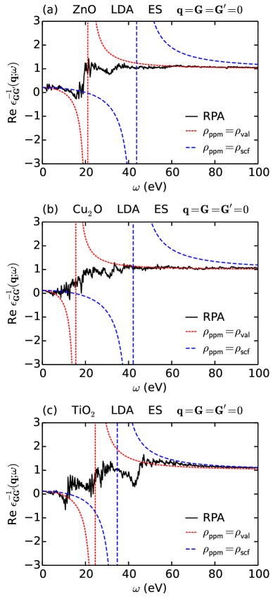
Figure 1: Real parts of inverse dielectric functions $\epsilon_{{\bf GG}^{\prime}}^{-1}{({\bf q};\omega)}$ at ${\bf q}={\bf G}={\bf G}^{\prime}={\bf 0}$ of (a) wurtzite ZnO, (b) cuprite Cu₂O, and (c) rutile TiO₂ in case of the LDA starting point and experimental structural parameters (ES) calculated within the RPA (solid black) and constructed using the HL PPM with $\rho_{\mathrm{ppm}}=\rho_{\mathrm{val}}$ (short-dashed red) and $\rho_{\mathrm{ppm}}=\rho_{\mathrm{scf}}$ (long-dashed blue). The HL PPM mode frequencies $\tilde{\omega}_{{\bf GG}^{\prime}}{({\bf q})}$ are shown by the vertical dashed lines at (a) 21.0 eV and 43.8 eV, (b) 15.6 eV and 42.1 eV, and (c) 24.6 eV and 34.7 eV.

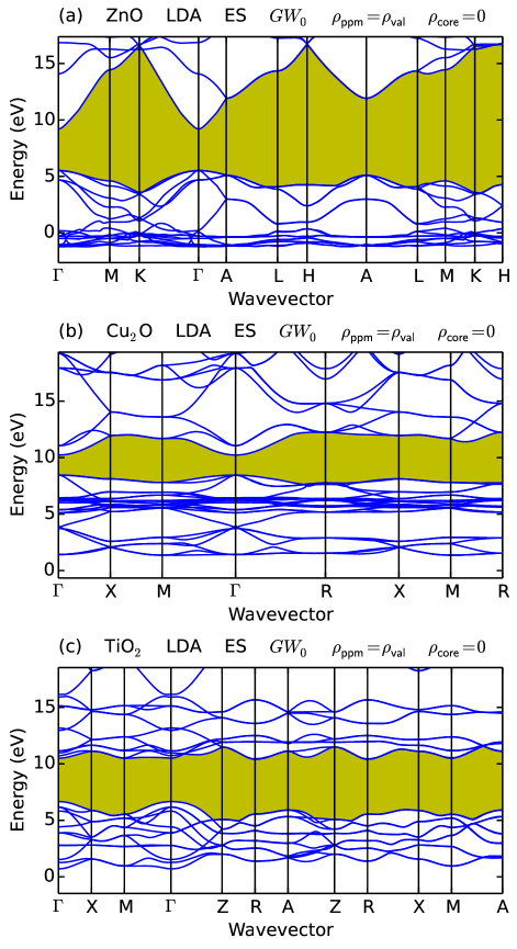
Figure 2: Quasiparticle band structures of (a) wurtzite ZnO, (b) cuprite Cu₂O, and (c) rutile TiO₂ calculated using the LDA starting point, experimental structural parameters (ES), the eigenvalue self-consistent $GW_{0}$ scheme, the HL PPM with $\rho_{\mathrm{ppm}}=\rho_{\mathrm{val}}$, and matrix elements of $V_{\mathrm{xc}}$ without NLCC ($\rho_{\mathrm{core}}=0$). The zero reference for the energy scale is the average (${\bf G}={\bf 0}$ component) electrostatic (ionic plus Hartree) potential. The ${\bf k}$-point labeling is from Ref. Setyawan and Curtarolo, 2010. The band gaps are shaded in yellow.

To examine the effects of different approximations discussed in Sec. II on the quasiparticle band gaps and band edges of TMOs, we perform a series of calculations for wurtzite ZnO, cuprite Cu₂O, and rutile TiO₂ using Quantum ESPRESSO Giannozzi et al. (2009) and BerkeleyGW Deslippe et al. (2012) codes for the DFT and $GW$ parts, respectively. Calculations are carried out for the spin-unpolarized case with the local density approximation (LDA) in the PW form Perdew and Wang (1992) and the generalized gradient approximation (GGA) in the PBE form Perdew et al. (1996) for the exchange-correlation functional. Norm-conserving pseudopotentials are generated in a separable non-local form Kleinman and Bylander (1982) using the RRKJ scheme Rappe et al. (1990) and including scalar relativistic corrections and non-linear core corrections (NLCC) Louie et al. (1982). The pseudopotential parameters are summarized in Table 1. Convergence studies with respect to the size of the Monkhorst-Pack grid Monkhorst and Pack (1976), kinetic energy cutoffs, and the number of unoccupied Kohn-Sham bands used in the calculation of $\epsilon$ and $\Sigma$ are reported elsewhere Shih et al. (2010); Friedrich et al. (2011); Stankovski et al. (2011); Deslippe et al. (2013); Malashevich et al. (2014). The parameters used in our calculations are summarized in Table 2. The Monkhorst-Pack grids for $\rho_{\mathrm{scf}}$, $\rho_{\mathrm{val}}$, and $\Sigma$ are $\Gamma$-centered and the ones for $\epsilon$ are shifted by half a grid spacing in all directions. A small wave vector along the (111) direction in crystal coordinates is used to calculate $\epsilon$ at the $\Gamma$ point. The convergence of $\Sigma$ with respect to the size of the Monkhorst-Pack grid is accelerated by averaging $v$ and $W$ inside the Voronoi cells of the $\left(\mathbf{k}+\mathbf{G}\right)$-points near the $\Gamma$-point Deslippe et al. (2012). The convergence of $\Sigma$ with respect to the number of unoccupied Kohn-Sham bands is accelerated by using the static remainder correction Deslippe et al. (2013). To ensure convergence of the stress tensor, structural relaxations are performed using 3 times higher kinetic energy cutoffs than those listed in Table 2. The experimental and theoretical structural parameters (thereafter referred to as ES and TS, respectively) are listed in Table 3.

Special consideration is required when constructing $\rho_{\mathrm{val}}$ used in the HL PPM. Given the two formula units per primitive cell and the electronic valence configurations listed in Table 1, ZnO, Cu₂O, and TiO₂ have 26, 44, and 24 valence bands, respectively. The top of the valence manifold is derived from the oxygen 2p⁶ states: bands 21–26 in ZnO, bands 39–44 in Cu₂O, and bands 13–24 in TiO₂. The lower valence bands are derived from the oxygen 2s² states and the transition metal third shell: bands 1–20 from O 2s² & Zn 3s²3p⁶3d¹⁰ in ZnO, bands 1–38 from O 2s² & Cu 3s²3p⁶3d¹⁰ in Cu₂O, and bands 1–12 from O 2s² & Ti 3s²3p⁶ in TiO₂. In TiO₂ the oxygen 2p states are separated from the transition metal 3d states by an energy gap, while in ZnO and Cu₂O they overlap. These overlapping states should be decoupled in order to unambiguously construct $\rho_{\mathrm{val}}$ from the oxygen 2p⁶ states. For that purpose we employ the DFT+U method with the following parameters: $U=8.0$ eV and $J=0.9$ eV for ZnO Shih et al. (2010); $U=7.5$ eV and $J=0.98$ eV for Cu₂O Heinemann et al. (2013). Note that the DFT+U method is only used for constructing $\rho_{\mathrm{val}}$, while $GW$ calculations are carried out starting from DFT orbitals. To quantify the effect of $U$, we perform two sets of $GW$ calculations, one using DFT $\rho_{\mathrm{val}}$ and another using DFT+U $\rho_{\mathrm{val}}$. It is found that the inclusion of $U$ in $\rho_{\mathrm{val}}$ only changes the $GW$ band gaps by 10 meV and the $GW$ band edges by 40 meV. The much larger effect of using $\rho_{\mathrm{scf}}$ in the HL PPM will be discussed in Sec. IV.

Let us now describe the implementation of the eigenvalue self-consistent $GW_{0}$ scheme. Iterations on $E_{n\mathbf{k}}^{\mathrm{QP}}$ entering Eq. (2) are performed by explicitly calculating the matrix elements of $\Sigma$ and the values of $E_{n\mathbf{k}}^{\mathrm{QP}}$ for several valence and conduction bands near the band edges (16 valence and 14 conduction for ZnO, 26 valence and 10 conduction for Cu₂O, 12 valence and 16 conduction for TiO₂) and by applying the $\mathbf{k}$-dependent scissors operators to the lower valence and higher conduction bands. The $\mathbf{k}$-dependent scissor shifts are obtained from the lowest valence and highest conduction bands for which the matrix elements of $\Sigma$ and the values of $E_{n\mathbf{k}}^{\mathrm{QP}}$ are explicitly calculated. It is found that performing four iterations is sufficient to converge $E_{n\mathbf{k}}^{\mathrm{QP}}$ to within 10 meV.

IV Results and discussion

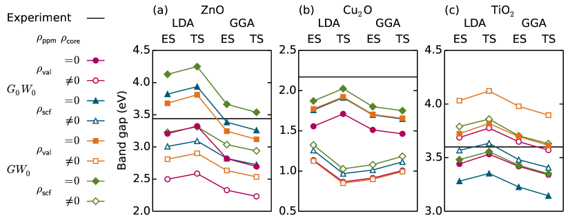
Figure 3: Quasiparticle band gaps of (a) wurtzite ZnO, (b) cuprite Cu₂O, and (c) rutile TiO₂ calculated within the $GW$ method and plotted as a function of the starting point (obtained from the LDA or GGA calculations) and of the structural parameters (either experimental or theoretical, labeled as ES and TS, respectively). Different symbols indicate the values calculated using different flavors of the $GW$ method, as shown in the legend on the left. The experimental band gaps taken from Refs. Reynolds et al., 1999; Baumeister, 1961; Rangan et al., 2010 are shown by horizontal lines.

Table 4: Band gaps of wurtzite ZnO measured using photoluminescence (PL) Reynolds et al. (1999) and calculated using DFT and $GW$. DFT and $GW$ band gaps are obtained using different exchange-correlation functionals (LDA and GGA), experimental and theoretical structural parameters (ES and TS), non-self-consistent $G_{0}W_{0}$ and eigenvalue self-consistent $GW_{0}$ schemes, HL PPM with $\rho_{\mathrm{ppm}}=\rho_{\mathrm{val}}$ and $\rho_{\mathrm{scf}}$, and matrix elements of $V_{\mathrm{xc}}$ without and with NLCC ($\rho_{\mathrm{core}}=0$ and $\neq 0$). The DFT and $GW$ band gaps are direct at the $\Gamma$ point. All values are in eV.

Wurtzite ZnO			LDA		GGA
	$\rho_{\mathrm{ppm}}$	$\rho_{\mathrm{core}}$	ES	TS	ES	TS
PL			3.44
DFT			0.74	0.80	0.85	0.78
$G_{0}W_{0}$	$\rho_{\mathrm{val}}$	$=0$	3.21	3.32	2.82	2.70
		$\neq 0$	2.50	2.59	2.33	2.23
	$\rho_{\mathrm{scf}}$	$=0$	3.82	3.94	3.38	3.26
		$\neq 0$	3.01	3.09	2.82	2.72
$GW_{0}$	$\rho_{\mathrm{val}}$	$=0$	3.68	3.81	3.24	3.12
		$\neq 0$	2.81	2.90	2.63	2.54
	$\rho_{\mathrm{scf}}$	$=0$	4.13	4.25	3.66	3.54
		$\neq 0$	3.23	3.31	3.04	2.94

Table 5: Band gaps of cuprite Cu₂O measured using optical absorption spectroscopy (OAS) Baumeister (1961) and calculated using DFT and $GW$. DFT and $GW$ band gaps are obtained using different exchange-correlation functionals (LDA and GGA), experimental and theoretical structural parameters (ES and TS), non-self-consistent $G_{0}W_{0}$ and eigenvalue self-consistent $GW_{0}$ schemes, HL PPM with $\rho_{\mathrm{ppm}}=\rho_{\mathrm{val}}$ and $\rho_{\mathrm{scf}}$, and matrix elements of $V_{\mathrm{xc}}$ without and with NLCC ($\rho_{\mathrm{core}}=0$ and $\neq 0$). The DFT and $GW$ band gaps are direct at the $\Gamma$ point. All values are in eV.

Cuprite Cu2O			LDA		GGA
	$\rho_{\mathrm{ppm}}$	$\rho_{\mathrm{core}}$	ES	TS	ES	TS
OAS			2.17
DFT			0.52	0.69	0.53	0.47
$G_{0}W_{0}$	$\rho_{\mathrm{val}}$	$=0$	1.56	1.71	1.51	1.46
		$\neq 0$	1.14	0.87	0.91	1.01
	$\rho_{\mathrm{scf}}$	$=0$	1.76	1.91	1.70	1.65
		$\neq 0$	1.26	0.97	1.01	1.11
$GW_{0}$	$\rho_{\mathrm{val}}$	$=0$	1.77	1.92	1.70	1.66
		$\neq 0$	1.13	0.85	0.90	0.99
	$\rho_{\mathrm{scf}}$	$=0$	1.87	2.03	1.80	1.75
		$\neq 0$	1.32	1.03	1.08	1.18

Table 6: Band gaps of rutile TiO₂ measured using photoemission spectroscopy (PES) Rangan et al. (2010) and calculated using DFT and $GW$. DFT and $GW$ band gaps are obtained using different exchange-correlation functionals (LDA and GGA), experimental and theoretical structural parameters (ES and TS), non-self-consistent $G_{0}W_{0}$ and eigenvalue self-consistent $GW_{0}$ schemes, HL PPM with $\rho_{\mathrm{ppm}}=\rho_{\mathrm{val}}$ and $\rho_{\mathrm{scf}}$, and matrix elements of $V_{\mathrm{xc}}$ without and with NLCC ($\rho_{\mathrm{core}}=0$ and $\neq 0$). The DFT and $GW$ band gaps are direct at the $\Gamma$ point (in regular font) and indirect between the $\Gamma$ point at the VBM and the R point at the CBM (in cursive font). All values are in eV.

Rutile TiO2			LDA		GGA
	$\rho_{\mathrm{ppm}}$	$\rho_{\mathrm{core}}$	ES	TS	ES	TS
PES			3.60
DFT			1.82	1.85	1.90	1.85
$G_{0}W_{0}$	$\rho_{\mathrm{val}}$	$=0$	3.44	3.53	3.42	3.34
		$\neq 0$	3.69	3.78	3.65	3.57
	$\rho_{\mathrm{scf}}$	$=0$	3.28	3.35	3.23	3.14
		$\neq 0$	3.57	3.63	3.48	3.41
$GW_{0}$	$\rho_{\mathrm{val}}$	$=0$	3.72	3.82	3.70	3.61
		$\neq 0$	4.03	4.12	3.98	3.90
	$\rho_{\mathrm{scf}}$	$=0$	3.48	3.56	3.43	3.35
		$\neq 0$	3.79	3.86	3.70	3.63

$GW$ calculations for wurtzite ZnO, cuprite Cu₂O, and rutile TiO₂ are performed using LDA and GGA starting points, experimental and theoretical structural parameters (ES and TS), non-self-consistent $G_{0}W_{0}$ and eigenvalue self-consistent $GW_{0}$ schemes, HL PPM with $\rho_{\mathrm{ppm}}$ set to DFT+U $\rho_{\mathrm{val}}$ and DFT $\rho_{\mathrm{scf}}$, and matrix elements of $V_{\mathrm{xc}}$ without and with NLCC ($\rho_{\mathrm{core}}=0$ and $\neq 0$). In the latter case, values of integrated partial core charge $q_{\mathrm{core}}=\int d\mathbf{r}\rho_{\mathrm{core}}{(\mathbf{r})}$ are listed in Table 1. Fig. 1 shows the real parts of $\epsilon_{\mathbf{00}}^{-1}{(\mathbf{0};\omega)}$ for the three TMOs in case of the LDA starting point and experimental structural parameters (ES) calculated within the RPA and constructed using the HL PPM with $\rho_{\mathrm{ppm}}=\rho_{\mathrm{val}}$ and $\rho_{\mathrm{scf}}$. Fig. 2 shows the quasiparticle band structures calculated using the LDA starting point, experimental structural parameters (ES), the eigenvalue self-consistent $GW_{0}$ scheme, the HL PPM with $\rho_{\mathrm{ppm}}=\rho_{\mathrm{val}}$, and matrix elements of $V_{\mathrm{xc}}$ without NLCC ($\rho_{\mathrm{core}}=0$). Fig. 3 shows the quasiparticle band gaps plotted as a function of the starting point (obtained from the LDA or GGA calculations) and of the structural parameters (either experimental or theoretical, labeled as ES and TS, respectively). Different symbols indicate the values calculated using different flavors of the $GW$ method. In this context, flavor refers to the choice of self-consistent scheme, $\rho_{\mathrm{ppm}}$, and $\rho_{\mathrm{core}}$. The experimental band gaps taken from Refs. Reynolds et al., 1999; Baumeister, 1961; Rangan et al., 2010 are shown for comparison. Tables 4-6 give the experimental and calculated band gaps plotted in Fig. 3 as well as the Kohn-Sham values not shown in Fig. 3. Kohn-Sham and quasiparticle band energies $E_{n\mathbf{k}}^{\mathrm{KS}}$ and $E_{n\mathbf{k}}^{\mathrm{QP}}$ and matrix elements of $V_{\mathrm{xc}}$ and $\Sigma$ at the valence band maximum (VBM) and conduction band minimum (CBM) are provided in Supplemental Material nlc .

Comparing Fig. 1(a) with Fig. 2(a) of Ref. Stankovski et al., 2011, Fig. 5(a) of Ref. Miglio et al., 2012, and Fig. 4(d) of Ref. Larson et al., 2013, we find that in the case of ZnO, the HL PPM becomes similar to the GN PPM when $\rho_{\mathrm{ppm}}$ is set to $\rho_{\mathrm{val}}$. One can see from Fig. 1 that for all three oxides, the HL PPM with $\rho_{\mathrm{ppm}}=\rho_{\mathrm{val}}$ gives a better fit to the RPA results than the HL PPM with $\rho_{\mathrm{ppm}}=\rho_{\mathrm{scf}}$. We note that the HL PPM suffers from the ambiguity of constructing the proper $\rho_{\mathrm{ppm}}$. This problem is absent in the GN PPM, suggesting that the HL PPM is more difficult to use for studying TMOs than the GN PPM.

Several conclusions can be drawn from statistical analysis of the data presented in Fig. 3 and Tables 4-6.

• Comparing the values in ($G_{0}W_{0}$, $\rho_{\mathrm{val}}$, $0$) row at (LDA, ES) and (GGA, ES) columns for ZnO, we find that the band gap varies by $3.21-2.82=0.39$ eV depending on the starting point (obtained from the LDA or GGA calculations). Averaging this quantity over different $\rho_{\mathrm{core}}=0$ rows for ZnO gives the mean variation in the band gap with different starting points as equal to 0.44 eV. Repeating this procedure for Cu₂O and TiO₂ yields the values of 0.06 eV and 0.04 eV, respectively. The large variation in the case of ZnO indicates that neither LDA nor GGA provides a good starting point for $GW$ calculations. At the same time, small variations for Cu₂O and TiO₂ imply that LDA and GGA give similar (but not necessarily good) starting points for $GW$ calculations. Other starting points were tried in $GW$ calculations for ZnO including DFT+U Shih et al. (2010), the screened hybrid functional Schleife et al. (2008), and the exact exchange optimized effective potential Yan et al. (2011). Note that the latter starting point can present some challenges in the subsequent $GW$ calculations Fleszar (2001). Overall, the problem of the starting point in $GW$ calculations for ZnO may require further research to give the full picture.

• Comparison of the values in $\rho_{\mathrm{core}}=0$ rows at (LDA, ES) and (LDA, TS) columns, as well as at (GGA, ES) and (GGA, TS) columns, shows that the variation of the band gap with the structural parameters is 0.12 eV for ZnO, 0.10 eV for Cu₂O, and 0.09 eV for TiO₂. This suggests that the band gaps are fairly insensitive to the structural parameters.

• Comparing the values in ($G_{0}W_{0}$, $\rho_{\mathrm{val}}$, $0$) and ($GW_{0}$, $\rho_{\mathrm{val}}$, $0$) rows, as well as in ($G_{0}W_{0}$, $\rho_{\mathrm{scf}}$, $0$) and ($GW_{0}$, $\rho_{\mathrm{scf}}$, $0$) rows, we find that the eigenvalue self-consistency in $G$ increases the band gap by 0.37 eV for ZnO, 0.16 eV for Cu₂O, and 0.24 eV for TiO₂. This is consistent with previous studies Shishkin and Kresse (2007).

• Comparison of the values in ($G_{0}W_{0}$, $\rho_{\mathrm{val}}$, $0$) and ($G_{0}W_{0}$, $\rho_{\mathrm{scf}}$, $0$) rows, as well as in ($GW_{0}$, $\rho_{\mathrm{val}}$, $0$) and ($GW_{0}$, $\rho_{\mathrm{scf}}$, $0$) rows, shows that the inclusion of core electrons in $\rho_{\mathrm{ppm}}$ increases the band gap of ZnO and Cu₂O by 0.51 and 0.15 eV, respectively, and decreases the band gap of TiO₂ by 0.22 eV. This is because for ZnO and Cu₂O, the VBM is lowered by a larger amount than the CBM, while the opposite scenario takes place for TiO₂, as follows from Supplemental Material nlc .

• Comparing the values in $\rho_{\mathrm{core}}=0$ and $\rho_{\mathrm{core}}\neq 0$ rows, we find that the inclusion of NLCC in the matrix elements of $V_{\mathrm{xc}}$ decreases the band gap of ZnO and Cu₂O by 0.70 and 0.69 eV, respectively, and increases the band gap of TiO₂ by 0.27 eV. This is due to the fact that for ZnO and Cu₂O, the VBM is raised by a larger amount than the CBM, while the opposite holds for TiO₂, as one can see from Supplemental Material nlc .

Overall, the largest variation of the band gap comes from the inclusion of NLCC in the matrix elements of $V_{\mathrm{xc}}$. This inclusion introduces significant errors in the calculated band gaps.

Fair agreement is found when comparing our results to those of previous $GW$ calculations for each oxide and specific flavor. In line with the criticism of the HL PPM Stankovski et al. (2011); Miglio et al. (2012); Larson et al. (2013), previous HL PPM calculations are compared to our $\rho_{\mathrm{ppm}}=\rho_{\mathrm{scf}}$ results, while previous GN PPM and non-PPM calculations to our $\rho_{\mathrm{ppm}}=\rho_{\mathrm{val}}$ results.

• For ZnO, we focus on (LDA, ES) column in Fig. 3(a) or Table 4. The most accurate non-PPM $G_{0}W_{0}$ calculations gave the following values for the band gap: 2.83 eV with the full potential linearized augmented plane wave (FLAPW) method Friedrich et al. (2011) and 2.87 eV with the projector augmented wave (PAW) method Klimeš et al. (2014). We find that the HL PPM gives a somewhat larger value of 3.21 eV and a substantially larger value of 3.82 eV when $\rho_{\mathrm{ppm}}$ is set to $\rho_{\mathrm{val}}$ and $\rho_{\mathrm{scf}}$, respectively. Previous HL PPM $G_{0}W_{0}$ calculations showed values in this range, 3.4 eV Shih et al. (2010), 3.57 eV Stankovski et al. (2011), and 3.56 eV Miglio et al. (2012), with one exception where the value of 2.80 eV was reported Larson et al. (2013). Other studies reported much lower values, such as non-PPM $G_{0}W_{0}$ band gaps of 2.17–2.43 eV Miglio et al. (2012); Larson et al. (2013) and the GN PPM $G_{0}W_{0}$ band gaps of 2.27–2.56 eV Stankovski et al. (2011); Miglio et al. (2012); Berger et al. (2012); Larson et al. (2013). We do not compare to the results of Refs. Shishkin and Kresse (2007); Fuchs et al. (2007); Kotani et al. (2007); Bechstedt et al. (2009); Hüser et al. (2013) which may be affected by the basis set convergence issues as discussed in Ref. Klimeš et al., 2014.

• For Cu₂O, let us look at (LDA, ES) column in Fig. 3(b) or Table 5. The ($G_{0}W_{0}$, $\rho_{\mathrm{val}}$, $0$) band gap of 1.56 eV compares with non-PPM $G_{0}W_{0}$ value of 1.34 eV Bruneval et al. (2006b). The ($GW_{0}$, $\rho_{\mathrm{val}}$, $0$) band gap of 1.77 eV is close to non-PPM eigenvalue self-consistent $GW$ band gap of 1.80 eV Bruneval et al. (2006b).

• For TiO₂, we start with (LDA, ES) column in Fig. 3(c) or Table 6. The ($G_{0}W_{0}$, $\rho_{\mathrm{val}}$, $0$) band gap of 3.44 eV is close to non-PPM $G_{0}W_{0}$ value of 3.34 eV Kang and Hybertsen (2010). We now move on to (GGA, TS) column. The ($G_{0}W_{0}$, $\rho_{\mathrm{val}}$, $0$) band gap of 3.34 eV is comparable to the GN PPM $G_{0}W_{0}$ value of 3.59 eV Chiodo et al. (2010). The ($G_{0}W_{0}$, $\rho_{\mathrm{scf}}$, $0$) band gap of 3.14 eV is close to the HL PPM $G_{0}W_{0}$ value of 3.13 eV Malashevich et al. (2014).

We now compare the calculated band gaps with the experimental data. The absolute difference of the experimental band gap and the value in ($G_{0}W_{0}$, $\rho_{\mathrm{val}}$, $0$) row at (LDA, ES) column for ZnO is equal to 0.23 eV. Averaging this quantity over the four columns in Fig. 3(a) or Table 4 gives the value of 0.43 eV. Further averaging over the three TMOs gives the mean deviation from experiment of 0.40 eV. This procedure is repeated for each flavor represented by different row in Fig. 3 and Tables 4-6. Among the eight flavors, the smallest deviation of 0.18 eV is found for ($GW_{0}$, $\rho_{\mathrm{val}}$, $0$) flavor, followed by the 0.30 eV deviation for ($GW_{0}$, $\rho_{\mathrm{scf}}$, $0$) flavor, the 0.31 eV deviation for ($G_{0}W_{0}$, $\rho_{\mathrm{scf}}$, $0$) flavor, and the 0.40 eV deviation for ($G_{0}W_{0}$, $\rho_{\mathrm{val}}$, $0$) flavor. Corresponding deviations for $\rho_{\mathrm{core}}\neq 0$ rows fall within the 0.49 to 0.78 eV range. We conclude that the best overall agreement with experiment is obtained for ($GW_{0}$, $\rho_{\mathrm{val}}$, $0$) flavor. On the other hand, we note from Fig. 3 that ($GW_{0}$, $\rho_{\mathrm{val}}$, $0$) values irregularly underestimate and overestimate the experimental band gaps, while ($G_{0}W_{0}$, $\rho_{\mathrm{val}}$, $0$) values always underestimate the experiment, suggesting that the latter flavor may be preferable to the former. Yet this conclusion may be deceiving given that the HL PPM with $\rho_{\mathrm{val}}$ overestimates the non-PPM band gap of ZnO by 0.34–0.38 eV (see the comparison with the previous calculations above) and that the experimental band gaps are renormalized by electron-phonon interaction not included in our calculations. Overall, it may be premature to conclude which flavor is preferable for TMOs until the effect of the vertex correction on $GW$ band gaps of these materials is thoroughly studied.

V Summary

In summary, we quantify the effects of different approximations used in the $GW$ method on the band gaps and band edges for three TMOs: wurtzite ZnO, cuprite Cu₂O, and rutile TiO₂. It is found that the $GW$ band gap of ZnO is sensitive to the starting point obtained from the LDA or GGA calculations, suggesting that the Kohn-Sham orbitals differ from the quasiparticle orbitals. It is shown that the HL PPM becomes similar to the GN PPM and gives better agreement with the RPA when $\rho_{\mathrm{ppm}}$ is set to $\rho_{\mathrm{val}}$, that is, only the valence electrons are used to determine the effective bare plasma frequencies for the HL PPM. It is demonstrated that the theoretically justified choice of approximations, namely eigenvalue self-consistent $GW_{0}$ scheme, $\rho_{\mathrm{val}}$ in the HL PPM, and the proper treatment of the $V_{\mathrm{xc}}$ term, give the best overall agreement between the calculated and measured band gaps.