Higgs-boson production through gluon fusion at NNLO QCD with parton showers
Abstract
We discuss how the UN2LOPS scheme for matching NNLO calculations to parton showers can be applied to processes with large higher-order perturbative QCD corrections. We focus on Higgs-boson production through gluon fusion as an example. We also present an NNLO fixed-order event generator for this reaction.
I Introduction
The high precision of experimental measurements at the Large Hadron Collider (LHC) requires equally precise theoretical calculations for the Standard Model processes of interest, such as Higgs-boson production Dittmaier et al. (2011); *Dittmaier:2012vm; *Heinemeyer:2013tqa. Experimental analyses often impose intricate kinematical cuts on the final-state phase space, thus calling for fully differential predictions of the cross section. At the same time the resummation of large logarithmic corrections is important, especially in order to describe QCD radiative corrections to the hard process.
These requirements have inspired many new techniques to simulate the structure of hadron collider events with unprecedented accuracy Buckley et al. (2011). Among them are the pioneering matching methods MC@NLO Frixione and Webber (2002) and POWHEG Nason (2004); *Frixione:2007vw, which allowed, for the first time, to combine next-to-leading order (NLO) QCD calculations with parton showers by means of a modified subtraction scheme. Even higher precision is needed for Higgs physics, as the dominant production mode through gluon fusion suffers from large perturbative corrections. Next-to-next-to leading order (NNLO) accurate fixed-order predictions Anastasiou and Melnikov (2002); *Harlander:2002wh; *Anastasiou:2005qj; Catani and Grazzini (2007a); Grazzini (2008); *Catani:2008me are routinely employed, NNLO accurate predictions for Higgs plus jet production have been obtained Boughezal et al. (2013) and N3LO accurate results are actively pursued Anastasiou et al. (2013); *Kilgore:2013gba; *Anastasiou:2014vaa; *Ball:2013bra; *Li:2013lsa; *Duhr:2013msa; *Li:2014bfa. Mixed QCD and electroweak two-loop corrections have been estimated assuming complete factorization Actis et al. (2008) and later evaluated in an effective theory approach Anastasiou et al. (2009a). Resummed predictions have been made at NNLO+NNLL accuracy de Florian and Grazzini (2009); *deFlorian:2012mx; Becher et al. (2013a), and jet vetoed cross sections, particularly relevant for Higgs boson decay channels involving bosons have been in the focus of interest recently Banfi et al. (2012a); *Banfi:2012jm; *Bonvini:2014joa; *Stewart:2013faa; *Becher:2012qa; *Becher:2013xia. The matching of NNLO fixed-order results to parton showers using the MINLO method was presented in Hamilton et al. (2013a); *Hamilton:2013fea.
Making the most precise fixed-order predictions available in the framework of general purpose event generators is a challenging task. Three different proposals exist for matching NNLO calculations to parton showers Lavesson and Lönnblad (2008); Hamilton et al. (2013a); *Hamilton:2013fea; Alioli et al. (2014), but only two of them were implemented so far Lavesson and Lönnblad (2008); Hamilton et al. (2013a); *Hamilton:2013fea; Höche et al. (2014); Karlberg et al. (2014). The aim of this publication is to discuss one of them, the UN2LOPS matching method, for Higgs boson production at hadron colliders. We also present an independent, fully differential NNLO fixed-order calculation of Higgs-boson production using the -cutoff technique.
This article is organized as follows: Section II reviews the UN2LOPS matching method. Section III discusses the implementation of the NNLO calculation. Alterations of the UN2LOPS proposal Höche et al. (2014), needed for the matching in Higgs production are introduced in Sec. IV. Section V presents our results and Sec. VI gives an outlook.
II UN2LOPS matching
To set the stage, we recall the refined UN2LOPS method Lönnblad and Prestel (2013) introduced in Höche et al. (2014). We assume MC@NLO matched predictions Frixione and Webber (2002), for Higgs-boson plus zero and one jets, which are to be merged. Any infrared safe observable is computed in these simulations as
| (1) |
where denotes the differential -particle phase space element, including a convolution with the PDFs. We use the following notation for the NLO-weighted Born cross section, , and the hard remainder function, :
| (2) |
The functions , and represent the Born, virtual, and real subtraction contribution to the -jet NLO calculation, while stands for the integrated subtraction terms Höche et al. (2012). represents the one-emission differential phase-space element, which factorizes as , with a Jacobian factor.
The generating functional of the parton shower, , is defined using the parton-shower evolution kernels, .
| (3) |
The no-branching probability, , follows from the unitarity condition . We use the abbreviations and to denote the evolution scales for the -particle process and the additional emission generated in the integration over . Similarly, we define a generating functional for the MC@NLO .
| (4) |
We restrict real corrections in the zero-jet MC@NLO to transverse momenta (denoted by by ), and we choose such that it falls below the parton-shower cutoff, . At the same time the one-jet calculation is regularized by requiring Higgs-boson transverse momenta larger than . This implies that resolved real corrections are generated solely by the one-jet MC@NLO . In order to reproduce the logarithmic structure of the parton-shower prediction, the emission terms must be weighted by the all-order resummed virtual and unresolved corrections Amati et al. (1980), which are obtained in form of a no-branching probability computed by the parton shower. At the same time, coupling renormalization and some higher-logarithmic corrections Dokshitzer et al. (1978); *Amati:1978by; *Ellis:1978sf; *Libby:1978ig; *Mueller:1978xu; *Dokshitzer:1978hw; Catani et al. (1991) are accounted for by reweighting with the appropriate ratio of coupling constants. This reweighting introduces terms that impair the NLO accuracy. They are subtracted by the first-order expansion of the weight factor, and by the first-order expansion of the no-branching probability, Höche et al. (2014).
| (5) |
We have defined and the regular and exceptional parts of the real corrections, and . They correspond to two-parton configurations with and without a parton-shower equivalent, respectively Höche et al. (2014). defines the resummation scale. The weight factor is given as
| (6) |
and where and denote the PDFs associated with the external and intermediate parton (in the sense of a parton-shower history). The scale factor includes effects of the 2-loop cusp anomalous dimension in the parton shower Kodaira and Trentadue (1983); *Catani:1989ne; *Catani:1988vd; *Catani:1992ua; Catani et al. (1991).
The restricted zero-jet calculation and the one-jet MC@NLO result above do not overlap. We can thus replace the zero-jet MC@NLO by a full -vetoed NNLO calculation, using the cutoff method Gao et al. (2013), and complete the cross section using the one-jet MC@NLO Höche et al. (2014): Each event removed from the one-jet bin by means of the emission probability is added to the zero-jet bin. This unitarization procedure is equivalent to a parton-shower resummation of the jet veto cross section at . It gives the UN2LOPS matching formula
| (7) |
where represents the -vetoed NNLO cross section, differential in the Born phase space. By construction the inclusive cross section exactly reproduces the NNLO result.
III The -vetoed NNLO calculation
In the dominant production mode at hadron colliders, the Higgs boson couples to two gluons via heavy quark loops. The full top and bottom quark mass dependent gluon fusion cross section is known to NLO only Spira (1997); *Anastasiou:2009kn. It is more convenient to work in an effective theory (HEFT), where the heavy top quark is integrated out Ellis et al. (1976); *Wilczek:1977zn; *Shifman:1979eb; *Ellis:1979jy. The gluon fusion process is then described by the effective Lagrangian,
| (8) |
where is the Higgs vacuum expectation value, and is the Wilson coefficient. Quark mass effects can be incorporated a posteriori. The matching to the Higgs effective theory leads to a factorized form of the hard function. We write it schematically as,
| (9) |
The hard function can be improved by including an addition overall factor of the full top mass dependent LO gluon fusion cross section, normalized by the HEFT LO cross section. This is a very good approximation at NNLO Pak et al. (2010); Harlander and Ozeren (2009); *Harlander:2009my. The hard function is applied to the NNLO results of effective theory order by order in , i.e. only multiplies the LO HEFT cross section, multiplies the NLO HEFT cross section, and multiplies the NNLO HEFT cross section. A similar scheme can be used in the matched calculation. However, we can also multiply the hard function as an overall factor to the HEFT calculation, leading to a second possible matching scheme, which will be discussed in Sec. IV.
The NNLO Higgs production in the Higgs effective theory implemented in Sherpa is based on the subtraction method Catani and Grazzini (2007a); Catani et al. (2009). It separates the two-loop NNLO calculation into a zero- bin, leaving the phase space with finite to the NLO calculation. This matches well with the general structure of UN2LOPS , introduced in Sec. II. The dependence on the cutoff, used to define the zero- bin, cancels between contributions from the two phase space regions. Given a small enough cutoff, the zero- bin can be mapped onto the Born phase space, as all soft and collinear radiation is integrated over. For Higgs or Drell Yan processes, where there is no final state colored particle at Born level, the cut roughly corresponds to the parton shower cutoff scale. In addition, the zero- bin follows a simple factorization formula, which generates very compact results for that can easily be implemented numerically. The remainder is computed as Higgs-boson plus one-jet production at NLO, using Ravindran et al. (2002) for the virtual matrix elements and the Catani-Seymour subtraction method for regularizing real radiative corrections Catani and Seymour (1997).
As a consequence of the factorization, the zero- bin contribution can be written as a differential K factor to the Born level cross section
| (10) |
where is the hard collinear coefficient, and refers to the PDF. The factorization formula describes the vetoed Higgs NNLO cross section up to power corrections in the cutoff, .
The hard collinear coefficient is derived using the framework developed in Becher et al. (2013a) and using recent two loop results given in Gehrmann et al. (2014a); *Gehrmann:2014uaa. The results have been verified against those presented in Catani and Grazzini (2012). In the framework of Sherpa, our implementation is fully differential in phase space, which allows to generate events at the parton level. Additionally, Higgs-boson decays to arbitrary final states can be included.
IV UN2LOPS in Higgs-boson production
Higgs-boson production via gluon fusion suffers from large perturbative corrections, both to the inclusive cross section and to the shape of distributions like the transverse momentum of the Higgs boson. This necessitates a careful treatment of higher-order effects in the matching to parton showers. In processes like Drell-Yan lepton pair production – where perturbative corrections to the transverse momentum distribution are small – different matching schemes will lead to similar results in the sense that any possible difference cannot be resolved experimentally. The situation is just the opposite in Higgs boson production, which was pointed out in several comparisons of NLO matching methods Alioli et al. (2009); Höche et al. (2012); Nason and Webber (2012). We discuss the problem in this section, and we propose two different strategies to tackle processes with large higher-order corrections.
Equation (7) proposes to subtract the no-branching probabilities, , only when they multiply the leading-order part, , of the one-jet MC@NLO result. This is a minimal approach. The expansion of the no-branching probabilities in powers of the strong coupling generates terms of when multiplied by or , which is beyond the required NNLO accuracy of UN2LOPS . It is thus acceptable to also subtract these no-branching probabilities. A factorization of the subtractions of and multiplying the term also only amounts to changing orders beyond the formal accuracy:
| (11) |
Finally, evaluating PDFs and in with running scales is legitimate. We will redefine in this way below. After these changes, the revised UN2LOPS matching formula reads
| (12) |
This again integrates to the NNLO cross section, while preserving the parton shower accuracy as well as the 1-jet NLO result up to higher orders in . The changes to the one-jet contribution of the UN2LOPS formula may be interpreted as a complete subtraction of contributions from the parton shower, where the branching probability, , is the natural expansion parameter of the resummation. Compared to the procedure described in Höche et al. (2014), we obtain the following additional contribution to the 1-jet bin:
| (13) |
These terms are clearly beyond the formal accuracy of the UN2LOPS method. Including them emphasizes the fixed-order result at medium and therefore removes some arbitrariness introduced by the parton shower resummation. It can thus be expected to be an improvement over the method presented in Höche et al. (2014), even though a thorough assessment can only be made after matching to N3LO fixed-order results. The implementation of Eq. (12) in a Monte-Carlo event generator is described in Appendix A.
In Eq. (12), does not affect exclusive observables. However, the hard function coming from the square of Wilson coefficients of the Higgs effective theory in are universal, and they should in fact appear also in differential distributions at higher orders, as they factorize from real-radiative corrections. It might be beneficial to single out such contributions. We therefore define two variants of the UN2LOPS method, which use the Wilson coefficients to improve the simulation of the one-jet process. This is very similar to the MC@NLO and POWHEG methods, as discussed in Höche et al. (2014).
The two possible ways of dealing with the factorized hard function are:
-
•
‘individual’ matching
-
–
Terms multiplying are matched using UN2LOPS
-
–
Terms multiplying are matched using MC@NLO
-
–
Terms multiplying are showered
-
–
-
•
‘factorized’ matching
-
–
The NNLO result in HEFT, ignoring the Wilson coefficient, is matched using UN2LOPS
-
–
The matched result is multiplied by in Eq. (9)
-
–
Note that the factorized matching increases the cross section by a few percent (see Sec. V). This increase can legitimately be considered as part of the large NNLO theoretical uncertainty in the Higgs-production process.
V Results
| 7 TeV | 14 TeV | 33 TeV | 100 TeV | |||||||||
|---|---|---|---|---|---|---|---|---|---|---|---|---|
| HNNLO | 13. | 494(7) | pb | 44. | 550(16) | pb | 160. | 84(13) | pb | – | ||
| SHERPA | 13. | 515(7) | pb | 44. | 559(36) | pb | 160. | 39(17) | pb | 670. | 1(10) | pb |
HNNLO
This section presents results using an implementation of the UN2LOPS algorithm in the event generator Sherpa Gleisberg et al. (2004); *Gleisberg:2008ta. We use a parton shower Schumann and Krauss (2008) based on Catani-Seymour dipole subtraction Catani and Seymour (1997); *Catani:2002hc. NLO virtual corrections for the one-jet process Ravindran et al. (2002) are taken from MCFM Campbell and Ellis (2010); *MCFM. Dipole subtraction is performed using Amegic Krauss et al. (2002); *Gleisberg:2007md and cross-checked with Comix Gleisberg and Höche (2008). We use the MSTW 2008 PDF set Martin et al. (2009) and the corresponding definition of the running coupling. We work in the five flavor scheme. Electroweak parameters are given as , . The results are derived in the limit . Predictions for finite will be given elsewhere.
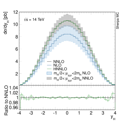
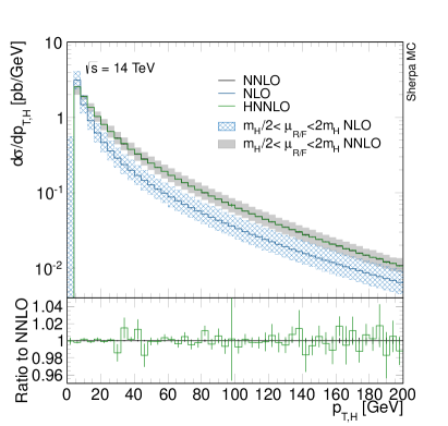
In order to cross-check our implementation we first compare the total cross section to results obtained from HNNLO Catani and Grazzini (2007a); Grazzini (2008); *Catani:2008me. Table 1 shows that the predictions agree within the permille-level statistical uncertainty of the Monte-Carlo integration. Additionally, we have checked that our results are identical when varying between 0.1 GeV and 1 GeV. The default value is 1 GeV. Figure 1 shows a comparison of the Higgs rapidity and transverse momentum spectrum between Sherpa and HNNLO . The excellent agreement over a wide range of phase space confirms the correct implementation of the NNLO calculation in Sherpa.
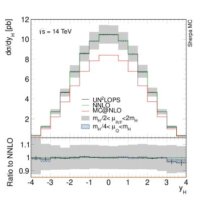
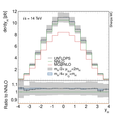
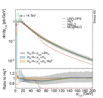
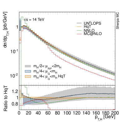
Figure 2 compares fixed-order predictions for the rapidity spectrum of the Higgs boson to matched results from UN2LOPS . Both the individual and factorized matching approach, introduced in Sec. IV yield perfect agreement for the shape of the distribution, while the factorized matching also slightly increases the cross section (see Sec. IV).
Figure 3 compares the UN2LOPS matched results for the Higgs boson transverse momentum to predictions from HqT Bozzi et al. (2003); *Bozzi:2005wk; *deFlorian:2011xf, which performs an analytic matching of the spectrum at NLO+NNLL accuracy. As expected, the resummation uncertainty in UN2LOPS is larger. Nevertheless, the central predictions agree quite well. This indicates that the impact of possible higher logarithmic contributions should be small enough to be neglected for the purpose of event generation at the 14 TeV LHC, provided that the central resummation scale is set appropriately. Similar findings were reported for production in Corke and Sjöstrand (2010).
The zero- bin is clearly problematic. This can be understood as follows: In our calculation the spectrum is described only at NLO+NLL accuracy Catani et al. (1991); Plätzer and Gieseke (2011). Therefore it suffers from large scale variations, particularly in the soft and collinear region. Equation 12 implies that an increased veto probability in this region also increases the cross section in the zero- bin. The large variation at zero- should thus be reduced significantly once the parton shower is amended with higher-logarithmic resummation. Note, however, that no such variation is present for inclusive observables like the Higgs-boson rapidity spectrum, Fig. 2.
VI Conclusions
We presented the first application of the UN2LOPS matching procedure to Higgs-boson production through gluon fusion. This reaction suffers from large higher-order corrections, and several refinements of the original UN2LOPS approach are suggested to improve the matching. They allow to obtain phenomenologically useful results despite the low logarithmic accuracy of the parton shower compared to analytic approaches. Our predictions are in fair agreement with higher logarithmic resummation for a resummation scale of .
We also provide an independent implementation of a fully differential NNLO calculation of Higgs-boson production at hadron colliders, using the -cutoff method, which allows the production of LHEF files Alwall et al. (2007); *Butterworth:2014efa or NTuple files Brun and Rademakers (1997); *Bern:2013zja containing NNLO event information at parton level.
Due to the fully exclusive nature of our simulations, it is straightforward to combine them with higher-multiplicity NLO calculations using an extension of the MENLOPS method Hamilton and Nason (2010); *Hoeche:2010kg to NNLO. This can be achieved by separating the generating functionals into a hard and a soft part and using appropriately weighted NLO calculations in the hard jet domain. A similar scheme, which also preserves the total cross section, could be based on the UNLOPS method Lönnblad and Prestel (2013); Plätzer (2013). Such a simulation will improve upon our predictions as soon as the Higgs-boson plus two-jet process is included at NLO. We leave the detailed study of the phenomenological implications to future work.
Acknowledgments
We thank Marek Schönherr and Thomas Lübbert for discussions and Valentin Hirschi and Gionata Luisoni for careful cross-checks of the virtual corrections to Higgs plus one-jet production. We are indebted to Lance Dixon, Frank Krauss, Leif Lönnblad and HuaXing Zhu for helpful conversations and comments on the manuscript. This work was supported by the US Department of Energy under contract DE–AC02–76SF00515. We used resources of the National Energy Research Scientific Computing Center, which is supported by the Office of Science of the U.S. Department of Energy under Contract No. DE–AC02–05CH11231.
Appendix A UN2LOPS step-by-step
This appendix provides a step-by-step guide to the UN2LOPS method, which allows to implement the technique in other processes of interest. We focus on reactions at hadron colliders, the generalization to lepton colliders being a straightforward modification. We assume that a vetoed NNLO cross section, computed along the lines of Sec. III exists. Any other method to provide this cross section can be used, for example a fully exclusive NNLO calculation restricted to by means of a veto.
-
1.
Generate a parton-level event according to , , or .
-
2.
If is selected, skip the parton shower step.
-
3.
If , of is selected, apply the clustering algorithm described in André and Sjöstrand (1998) to define a parton-shower history. If no history is found on events, they are classified as exceptional. In this case, simply run the parton shower starting from the two-particle state.
-
4.
In events, reweight with in Eq. (6) and subtract the first-order expansion, .
-
5.
Run a truncated parton shower on the zero-jet configuration as identified by backward clustering in step 3. Skip the first emission Höche et al. (2013). If the parton shower generates a second emission, reduce the one- or two-particle configuration to the zero-particle configuration identified in step 3 and do not apply any further parton shower or MC@NLO . If the parton shower does not generate a second emission, and the event was of type, perform the MC@NLO starting from the one-particle state. If the event was of type, run the parton shower, starting from the two-particle state.
References
- Dittmaier et al. (2011) S. Dittmaier et al. (LHC Higgs Cross Section Working Group), (2011), 10.5170/CERN-2011-002, arXiv:1101.0593 [hep-ph] .
- Dittmaier et al. (2012) S. Dittmaier et al. (LHC Higgs Cross Section Working Group), (2012), 10.5170/CERN-2012-002, arXiv:1201.3084 [hep-ph] .
- Heinemeyer et al. (2013) S. Heinemeyer et al. (LHC Higgs Cross Section Working Group), (2013), 10.5170/CERN-2013-004, arXiv:1307.1347 [hep-ph] .
- Buckley et al. (2011) A. Buckley et al., Phys. Rept. 504, 145 (2011), arXiv:1101.2599 [hep-ph] .
- Frixione and Webber (2002) S. Frixione and B. R. Webber, JHEP 06, 029 (2002), hep-ph/0204244 .
- Nason (2004) P. Nason, JHEP 11, 040 (2004), hep-ph/0409146 .
- Frixione et al. (2007) S. Frixione, P. Nason, and C. Oleari, JHEP 11, 070 (2007), arXiv:0709.2092 [hep-ph] .
- Anastasiou and Melnikov (2002) C. Anastasiou and K. Melnikov, Nucl.Phys. B646, 220 (2002), arXiv:hep-ph/0207004 [hep-ph] .
- Harlander and Kilgore (2002) R. V. Harlander and W. B. Kilgore, Phys.Rev.Lett. 88, 201801 (2002), arXiv:hep-ph/0201206 [hep-ph] .
- Anastasiou et al. (2005) C. Anastasiou, K. Melnikov, and F. Petriello, Nucl. Phys. B724, 197 (2005), arXiv:hep-ph/0501130 .
- Catani and Grazzini (2007a) S. Catani and M. Grazzini, Phys.Rev.Lett. 98, 222002 (2007a), arXiv:hep-ph/0703012 [hep-ph] .
- Grazzini (2008) M. Grazzini, JHEP 0802, 043 (2008), arXiv:0801.3232 [hep-ph] .
- Catani and Grazzini (2007b) S. Catani and M. Grazzini, PoS RADCOR2007, 046 (2007b), arXiv:0802.1410 [hep-ph] .
- Boughezal et al. (2013) R. Boughezal, F. Caola, K. Melnikov, F. Petriello, and M. Schulze, JHEP 06, 072 (2013), arXiv:1302.6216 [hep-ph] .
- Anastasiou et al. (2013) C. Anastasiou, C. Duhr, F. Dulat, F. Herzog, and B. Mistlberger, JHEP 1312, 088 (2013), arXiv:1311.1425 [hep-ph] .
- Kilgore (2013) W. B. Kilgore, (2013), arXiv:1312.1296 [hep-ph] .
- Anastasiou et al. (2014) C. Anastasiou, C. Duhr, F. Dulat, E. Furlan, T. Gehrmann, F. Herzog, and B. Mistlberger, (2014), arXiv:1403.4616 [hep-ph] .
- Ball et al. (2013) R. D. Ball, M. Bonvini, S. Forte, S. Marzani, and G. Ridolfi, Nucl.Phys. B874, 746 (2013), arXiv:1303.3590 [hep-ph] .
- Li and Zhu (2013) Y. Li and H. X. Zhu, JHEP 1311, 080 (2013), arXiv:1309.4391 [hep-ph] .
- Duhr and Gehrmann (2013) C. Duhr and T. Gehrmann, Phys.Lett. B727, 452 (2013), arXiv:1309.4393 [hep-ph] .
- Li et al. (2014) Y. Li, A. von Manteuffel, R. M. Schabinger, and H. X. Zhu, (2014), arXiv:1404.5839 [hep-ph] .
- Actis et al. (2008) S. Actis, G. Passarino, C. Sturm, and S. Uccirati, Phys.Lett. B670, 12 (2008), arXiv:0809.1301 [hep-ph] .
- Anastasiou et al. (2009a) C. Anastasiou, R. Boughezal, and F. Petriello, JHEP 04, 003 (2009a), arXiv:0811.3458 [hep-ph] .
- de Florian and Grazzini (2009) D. de Florian and M. Grazzini, Phys.Lett. B674, 291 (2009), arXiv:0901.2427 [hep-ph] .
- de Florian et al. (2012) D. de Florian, G. Ferrera, M. Grazzini, and D. Tommasini, JHEP 1206, 132 (2012), arXiv:1203.6321 [hep-ph] .
- Becher et al. (2013a) T. Becher, M. Neubert, and D. Wilhelm, JHEP 1305, 110 (2013a), arXiv:1212.2621 [hep-ph] .
- Banfi et al. (2012a) A. Banfi, G. P. Salam, and G. Zanderighi, JHEP 1206, 159 (2012a), arXiv:1203.5773 [hep-ph] .
- Banfi et al. (2012b) A. Banfi, P. F. Monni, G. P. Salam, and G. Zanderighi, Phys.Rev.Lett. 109, 202001 (2012b), arXiv:1206.4998 [hep-ph] .
- Bonvini and Marzani (2014) M. Bonvini and S. Marzani, (2014), arXiv:1405.3654 [hep-ph] .
- Stewart et al. (2013) I. W. Stewart, F. J. Tackmann, J. R. Walsh, and S. Zuberi, (2013), arXiv:1307.1808 .
- Becher and Neubert (2012) T. Becher and M. Neubert, JHEP 1207, 108 (2012), arXiv:1205.3806 [hep-ph] .
- Becher et al. (2013b) T. Becher, M. Neubert, and L. Rothen, JHEP 1310, 125 (2013b), arXiv:1307.0025 [hep-ph] .
- Hamilton et al. (2013a) K. Hamilton, P. Nason, C. Oleari, and G. Zanderighi, JHEP 1305, 082 (2013a), arXiv:1212.4504 .
- Hamilton et al. (2013b) K. Hamilton, P. Nason, E. Re, and G. Zanderighi, JHEP 1310, 222 (2013b), arXiv:1309.0017 [hep-ph] .
- Lavesson and Lönnblad (2008) N. Lavesson and L. Lönnblad, JHEP 12, 070 (2008), arXiv:0811.2912 [hep-ph] .
- Alioli et al. (2014) S. Alioli et al., JHEP 1406, 089 (2014), arXiv:1311.0286 [hep-ph] .
- Höche et al. (2014) S. Höche, Y. Li, and S. Prestel, (2014), arXiv:1405.3607 [hep-ph] .
- Karlberg et al. (2014) A. Karlberg, E. Re, and G. Zanderighi, (2014), arXiv:1407.2940 [hep-ph] .
- Lönnblad and Prestel (2013) L. Lönnblad and S. Prestel, JHEP 1303, 166 (2013), arXiv:1211.7278 [hep-ph] .
- Höche et al. (2012) S. Höche, F. Krauss, M. Schönherr, and F. Siegert, JHEP 09, 049 (2012), arXiv:1111.1220 [hep-ph] .
- Amati et al. (1980) D. Amati, A. Bassetto, M. Ciafaloni, G. Marchesini, and G. Veneziano, Nucl. Phys. B173, 429 (1980).
- Dokshitzer et al. (1978) Y. L. Dokshitzer, D. Diakonov, and S. Troian, (1978), SLAC-TRANS-0183.
- Amati et al. (1978) D. Amati, R. Petronzio, and G. Veneziano, Nucl. Phys. B146, 29 (1978).
- Ellis et al. (1978) R. K. Ellis, H. Georgi, M. Machacek, H. D. Politzer, and G. G. Ross, Phys.Lett. B78, 281 (1978).
- Libby and Sterman (1978) S. B. Libby and G. F. Sterman, Phys.Lett. B78, 618 (1978).
- Mueller (1978) A. H. Mueller, Phys.Rev. D18, 3705 (1978).
- Dokshitzer et al. (1980) Y. L. Dokshitzer, D. Diakonov, and S. I. Troian, Phys. Rept. 58, 269 (1980).
- Catani et al. (1991) S. Catani, B. R. Webber, and G. Marchesini, Nucl. Phys. B349, 635 (1991).
- Kodaira and Trentadue (1983) J. Kodaira and L. Trentadue, Phys.Lett. B123, 335 (1983).
- Catani and Trentadue (1989) S. Catani and L. Trentadue, Nucl. Phys. B327, 323 (1989).
- Catani et al. (1988) S. Catani, E. D’Emilio, and L. Trentadue, Phys.Lett. B211, 335 (1988).
- Catani et al. (1993) S. Catani, L. Trentadue, G. Turnock, and B. R. Webber, Nucl. Phys. B407, 3 (1993).
- Gao et al. (2013) J. Gao, C. S. Li, and H. X. Zhu, Phys.Rev.Lett. 110, 042001 (2013), arXiv:1210.2808 [hep-ph] .
- Spira (1997) M. Spira, Nucl.Instrum.Meth. A389, 357 (1997), arXiv:hep-ph/9610350 [hep-ph] .
- Anastasiou et al. (2009b) C. Anastasiou, S. Bucherer, and Z. Kunszt, JHEP 0910, 068 (2009b), arXiv:0907.2362 [hep-ph] .
- Ellis et al. (1976) J. R. Ellis, M. K. Gaillard, and D. V. Nanopoulos, Nucl.Phys. B106, 292 (1976).
- Wilczek (1977) F. Wilczek, Phys.Rev.Lett. 39, 1304 (1977).
- Shifman et al. (1979) M. A. Shifman, A. Vainshtein, M. Voloshin, and V. I. Zakharov, Sov.J.Nucl.Phys. 30, 711 (1979).
- Ellis et al. (1979) J. R. Ellis, M. Gaillard, D. V. Nanopoulos, and C. T. Sachrajda, Phys.Lett. B83, 339 (1979).
- Pak et al. (2010) A. Pak, M. Rogal, and M. Steinhauser, JHEP 1002, 025 (2010), arXiv:0911.4662 [hep-ph] .
- Harlander and Ozeren (2009) R. V. Harlander and K. J. Ozeren, JHEP 0911, 088 (2009), arXiv:0909.3420 [hep-ph] .
- Harlander et al. (2010) R. V. Harlander, H. Mantler, S. Marzani, and K. J. Ozeren, Eur.Phys.J. C66, 359 (2010), arXiv:0912.2104 [hep-ph] .
- Catani et al. (2009) S. Catani, L. Cieri, G. Ferrera, D. de Florian, and M. Grazzini, Phys.Rev.Lett. 103, 082001 (2009), arXiv:0903.2120 [hep-ph] .
- Ravindran et al. (2002) V. Ravindran, J. Smith, and W. Van Neerven, Nucl. Phys. B634, 247 (2002), hep-ph/0201114 .
- Catani and Seymour (1997) S. Catani and M. H. Seymour, Nucl. Phys. B485, 291 (1997), arXiv:hep-ph/9605323 .
- Gehrmann et al. (2014a) T. Gehrmann, T. Luebbert, and L. L. Yang, (2014a), arXiv:1403.6451 [hep-ph] .
- Gehrmann et al. (2014b) T. Gehrmann, T. Luebbert, and L. L. Yang, PoS RADCOR2013, 011 (2014b), arXiv:1401.1222 [hep-ph] .
- Catani and Grazzini (2012) S. Catani and M. Grazzini, Eur.Phys.J. C72, 2013 (2012), arXiv:1106.4652 [hep-ph] .
- Alioli et al. (2009) S. Alioli, P. Nason, C. Oleari, and E. Re, JHEP 04, 002 (2009), arXiv:0812.0578 [hep-ph] .
- Nason and Webber (2012) P. Nason and B. Webber, (2012), arXiv:1202.1251 [hep-ph] .
- Gleisberg et al. (2004) T. Gleisberg, S. Höche, F. Krauss, A. Schälicke, S. Schumann, and J. Winter, JHEP 02, 056 (2004), hep-ph/0311263 .
- Gleisberg et al. (2009) T. Gleisberg, S. Höche, F. Krauss, M. Schönherr, S. Schumann, F. Siegert, and J. Winter, JHEP 02, 007 (2009), arXiv:0811.4622 [hep-ph] .
- Schumann and Krauss (2008) S. Schumann and F. Krauss, JHEP 03, 038 (2008), arXiv:0709.1027 [hep-ph] .
- Catani et al. (2002) S. Catani, S. Dittmaier, M. H. Seymour, and Z. Trocsanyi, Nucl. Phys. B627, 189 (2002), hep-ph/0201036 .
- Campbell and Ellis (2010) J. M. Campbell and R. Ellis, Nucl.Phys.Proc.Suppl. 205-206, 10 (2010), arXiv:1007.3492 [hep-ph] .
- (76) J. Campbell, R. K. Ellis, and C. Williams, http://mcfm.fnal.gov.
- Krauss et al. (2002) F. Krauss, R. Kuhn, and G. Soff, JHEP 02, 044 (2002), hep-ph/0109036 .
- Gleisberg and Krauss (2008) T. Gleisberg and F. Krauss, Eur. Phys. J. C53, 501 (2008), arXiv:0709.2881 [hep-ph] .
- Gleisberg and Höche (2008) T. Gleisberg and S. Höche, JHEP 12, 039 (2008), arXiv:0808.3674 [hep-ph] .
- Martin et al. (2009) A. D. Martin, W. J. Stirling, R. S. Thorne, and G. Watt, Eur. Phys. J. C63, 189 (2009), arXiv:0901.0002 [hep-ph] .
- Bozzi et al. (2003) G. Bozzi, S. Catani, D. de Florian, and M. Grazzini, Phys.Lett. B564, 65 (2003), arXiv:hep-ph/0302104 [hep-ph] .
- Bozzi et al. (2006) G. Bozzi, S. Catani, D. de Florian, and M. Grazzini, Nucl. Phys. B737, 73 (2006), arXiv:hep-ph/0508068 .
- de Florian et al. (2011) D. de Florian, G. Ferrera, M. Grazzini, and D. Tommasini, (2011), arXiv:1109.2109 [hep-ph] .
- Corke and Sjöstrand (2010) R. Corke and T. Sjöstrand, Eur. Phys. J. C69, 1 (2010), arXiv:1003.2384 [hep-ph] .
- Plätzer and Gieseke (2011) S. Plätzer and S. Gieseke, JHEP 01, 024 (2011), arXiv:0909.5593 [hep-ph] .
- Alwall et al. (2007) J. Alwall et al., Comput. Phys. Commun. 176, 300 (2007), hep-ph/0609017 .
- Butterworth et al. (2014) J. Butterworth, G. Dissertori, S. Dittmaier, D. de Florian, N. Glover, et al., (2014), arXiv:1405.1067 [hep-ph] .
- Brun and Rademakers (1997) R. Brun and F. Rademakers, Nucl.Instrum.Meth. A389, 81 (1997).
- Bern et al. (2014) Z. Bern et al., Comput.Phys.Commun. 185, 1443 (2014), arXiv:1310.7439 [hep-ph] .
- Hamilton and Nason (2010) K. Hamilton and P. Nason, JHEP 06, 039 (2010), arXiv:1004.1764 [hep-ph] .
- Höche et al. (2011) S. Höche, F. Krauss, M. Schönherr, and F. Siegert, JHEP 08, 123 (2011), arXiv:1009.1127 [hep-ph] .
- Plätzer (2013) S. Plätzer, JHEP 1308, 114 (2013), arXiv:1211.5467 [hep-ph] .
- André and Sjöstrand (1998) J. André and T. Sjöstrand, Phys. Rev. D57, 5767 (1998), arXiv:hep-ph/9708390 .
- Höche et al. (2013) S. Höche, F. Krauss, M. Schönherr, and F. Siegert, JHEP 1304, 027 (2013), arXiv:1207.5030 [hep-ph] .