Large-$N_{c}$ naturalness in coupled-channel meson-meson scattering

Abstract

The analysis of hadronic interactions with effective field theory techniques is complicated by the appearance of a large number of low-energy constants, which are usually fitted to data. On the other hand, the large-$N_{c}$ limit helps to impose natural short-distance constraints on these low-energy constants, providing a parameter reduction. A Bayesian interpretation of the expected $1/N_{c}$ accuracy allows for an easy and efficient implementation of these constraints, using an augmented $\chi^{2}$. We apply this approach to the analysis of meson-meson scattering, in conjunction with chiral perturbation theory to one loop and coupled-channel unitarity, and show that it helps to largely reduce the many existing ambiguities and simultaneously provide an acceptable description of the available phase shifts.

I Introduction

While the solution of QCD remains a difficult and challenging problem which is being progressively tackled on the lattice, there are two limits where substantial simplifications apply in the continuum: the chiral limit Langacker:1973hh , where the current quark mass $m_{q}$ is set to zero (see Pich:1995bw ; Ecker:1994gg for a review), and the limit of a large number of colours $N_{c}$ 'tHooft:1973jz ; Witten:1979kh (see Ref. Lucini:2013qja for a recent review and references therein), where the strong coupling constant scales as $\alpha_{s}\sim 1/N_{c}$. The main common virtue of these simplifications is that at sufficiently low energies, $\sqrt{s}\leq\Lambda$, quark-hadron duality and confinement require that these limits and their corrections can be expressed in purely hadronic terms, with no explicit reference to the underlying quark and gluon degrees of freedom. A well-known example of this duality is given by the Gell-Mann–Oakes–Renner relation, $2m_{q}|\langle\bar{q}q\rangle|=f_{\pi}^{2}m_{\pi}^{2}$, which is ${\cal O}(N_{c}m_{\pi}^{2})$ and relates the current quark mass $m_{q}$ and the quark condensate $\langle\bar{q}q\rangle$ with the pion decay constant $f_{\pi}$ and the pion mass $m_{\pi}$.

Of course, none of these extreme limits are generally expected to faithfully feature the real world. Instead, the smallness of the quark mass as compared to $\Lambda_{\rm QCD}$ and the largeness of $N_{c}=3$ as compared to unity suggest a sensible hierarchy where an expansion in the $u,d,s$ quark masses and a $1/N_{c}$ expansion may be combined in a suitable way to attempt a credible description of hadron properties and their interactions. Within an effective Lagrangian approach Weinberg:1978kz , and using the low-energy degrees of freedom (Goldstone bosons) of the non-linear sigma model Appelquist:1980ae , a chiral perturbation theory ($\chi$PT) to one loop was thus designed Gasser:1983yg ; Gasser:1984gg . On the other hand, the leading tree-level structure implied by the large-$N_{c}$ limit suggests using a resonance chiral theory (R$\chi$T) to successfully saturate the low-energy properties Ecker:1988te ; Ecker:1989yg ; Cirigliano:2006hb . It has been shown that resonance saturation arises quite naturally Pich:2002xy from the short-distance constraints on the effective hadronic theory stemming from the underlying high-energy behaviour of QCD for space-like momenta.

This scheme is implemented in terms of chiral effective Lagrangians displaying explicitly the relevant hadronic degrees of freedom, characterized by i) a finite number of fields representing stable particles, in the large-$N_{c}$ limit, with masses $M_{R}={\cal O}(N_{c}^{0})\lesssim\Lambda$ , ii) ${\cal O}(m_{q})$ suppressed couplings to pseudoscalar-mesons and iii) $n-$mesonic ${\cal O}(N_{c}^{1-n/2})$ suppressed couplings. The decay rate of these states is suppressed, $\Gamma_{R}={\cal O}(N_{c}^{-1})$, and are thus resonances. The calculation of quantum corrections, besides restoring unitarity perturbatively within the relevant $\Lambda$-truncated Hilbert space, accounts for the scale dependence of the couplings in the Lagrangian, as they effectively and implicitly incorporate the degrees of freedom which have been integrated out. The number of low-energy couplings (LECs) depends on how many independent terms can be written in the effective Lagrangian with fields and their derivatives, so that they naturally scale with inverse powers of the breakdown scale $\Lambda$. As it is well known, this number grows rapidly with the order of the expansion, and predictive power relies heavily on having more data than couplings. Large-$N_{c}$ arguments have helped in fixing the bulk of the scale-independent contribution for the LECs at ${\cal O}(p^{4})$ and ${\cal O}(p^{6})$ (see however Kampf:2006bn for an exception at ${\cal O}(p^{6})$).

In this paper we are concerned with the implications of next-to-leading order (NLO) $\chi$PT and leading order (LO) $1/N_{c}$ corrections in the description of the interactions among pseudoscalar mesons belonging to the flavour octet and below a given energy cut-off, which will be set at $\sqrt{s_{\rm max}}\sim 1.1-1.2~{}\mathrm{GeV}\equiv\Lambda_{R}$ for definiteness. This energy cut-off provides a motivation to truncate the infinite tower of meson states to just one per quantum number (except for the $0^{++}$ scalar and $0^{-+}$ pseudo-scalar multiplets, where independent octet and singlet states are considered). At first order in the $1/N_{c}$ expansion, terms with more than one trace and loops are suppressed; therefore, we only include tree-level resonance contributions. Moreover, we neglect interactions between different resonance channels which, although allowed by the theory symmetries, are not needed in this work.

Furthermore, as argued in Ref. Nieves:2011gb , in addition to the tree-level meson-exchange diagrams, one should also foresee contact pieces, which depend on the high-energy cut-off $\Lambda_{R}$. In that work, $\Lambda_{R}\sim 700~{}\mathrm{MeV}$ and thus only elastic $\pi\pi$ scattering was possible. On the other hand, when $\Lambda_{R}\sim 1.2~{}\mathrm{GeV}$ all pseudoscalar-pseudoscalar channels are open; thus, coupled-channel unitarity plays a decisive role. We use here the Bethe-Salpeter equation (BSE) approach, within the on-shell renormalization scheme Nieves:1999bx conveniently extended to the coupled-channel case, which restores exact two-body unitarity, thereby enlarging the scope of the previous work Nieves:2011gb to include coupled channels. This BSE on-shell scheme is characterized by the appearance of non-perturbative subtraction constants, $C_{IJ}$, and a perturbative matching procedure to reproduce LO $1/N_{c}$ and NLO $\chi$PT. In all, we need 24 independent parameters which must be fixed from fitting scattering data or pseudo-data, a rather impractical situation. We will show how a judicious fitting strategy, based on the natural expectation that NLO $1/N_{c}$ corrections are at the $\sim 30\%$ level, provides good fits with reasonable parameters.

Before embarking into a more involved discussion, let us explain the main idea behind the present work. In the chiral limit, $m_{\pi}\to 0$, QCD has only one dimensionful parameter which can be chosen to be the pion weak decay constant, $f$. In the large-$N_{c}$ limit $f={\cal O}(\sqrt{N_{c}})$ and hence meson masses must scale as $M_{R}\sim f/\sqrt{N_{c}}$ and meson couplings as $G_{R}\sim f$. That means that we expect an expansion of the form,

$$\frac{\sqrt{N_{c}}M_{R}}{f}=a_{R}\left[1+\frac{\xi_{R}}{N_{c}}+\dots\right]$$ (1)

where $a_{R}$ and $\xi_{R}$ are numerical dimensionless coefficients of order one. The basic idea to be explored in the present work is the use of this information when we have a good estimate for the LO $a_{R}$, but no information on the NLO term $\xi_{R}$. Under these circumstances, we may assume that $\xi_{R}$ is a random variable normally distributed, $\langle\xi_{R}\rangle=0$ and $\langle\xi_{R}^{2}\rangle={\cal O}(1)$, in which case the variable (for simplicity couplings $G_{R}$ are omitted)

$$\chi^{2}_{\rm th}=\sum_{R}\xi_{R}^{2}\,,\qquad\xi_{R}=\frac{\sqrt{N_{c}}M_{R}/a_{R}-f}{f/N_{c}}$$ (2)

follows a $\chi^{2}$ distribution if the different $\xi_{R}$’s are uncorrelated, $\langle\xi_{R}\xi_{R}^{\prime}\rangle=\delta_{R,R^{\prime}}\langle\xi_{R}^{2}\rangle$. In the absence of further information, $\chi^{2}$ is minimized by our guess of the parameters $M_{R}$ and $G_{R}$. However, if we have further data which can be described theoretically by these parameters, $M_{R},G_{R}$, we may refine our initial guess by adding to Eq. (2) the standard $\chi^{2}$ term used to carry out a fit to these data. In the first part of the paper we will analyze how the LO coefficients can be estimated. In the second part we will show how to profit from these estimates in meson-meson scattering.

The paper is organized as follows. In Section II we discuss and motivate short-distance constraints in the large-$N_{c}$ limit and their consequences in the light of data and lattice studies. In Section III we analyze how the naturalness of leading $1/N_{c}$ corrections provides a sensible estimate on the expected uncertainties of low-energy constants. The formalism for coupled-channel unitarized meson-meson scattering and some specific features are reviewed in Section IV. Our fitting strategies and main numerical results are presented in Section V. Finally, in Section VI we summarize our points and come to the conclusions.

II Large-$N_{c}$ short-distance constraints

II.1 Motivation

In this section we analyze some important conditions which arise from imposing the best possible high-energy behaviour of field correlators in a low-energy truncated hadronic theory, compatible with the known behaviour in QCD. This leads to a sensible parameter reduction, based on estimates of $a_{R}$ in Eq. (1), which will be very helpful in our analysis of meson-meson scattering. These short-distance constraints are obtained within a large-$N_{c}$ framework and when the low-energy theory is limited to spin 0 and 1 resonances, and allow for a complete parameter reduction in the chiral limit; all couplings and masses can be explicitly expressed in terms of the pion weak decay constant and the number of colours $N_{c}$. In order to appreciate the result, it is important to spell out which are the main assumptions and approximations leading to it.

As already mentioned, in the large-$N_{c}$ limit interactions among hadrons and with external currents are suppressed. This allows to set up a hierarchy in terms of an infinite number of quantum hadronic fields $R_{i}(x)$ and their derivatives, compatible with the symmetries at all energies, which can be written at tree level in terms of a real local Lagrangian with a given set of coupling constants $G_{R_{i}}$ and hadron masses $M_{R_{i}}$. Unitarity is recovered perturbatively by computing quantum corrections in a loop expansion. As we are interested in an intermediate energy description, say $\sqrt{s}\leq\Lambda_{R}$, we need only to consider explicitly a finite number of fields which are active below this cut-off scale, $M_{R_{i}}\lesssim\Lambda_{R}$. Heavier states, $\Lambda_{R}\lesssim M_{R_{i}}$ are included implicitly through the couplings $G_{R_{i}}(\Lambda,M_{R_{i}})$ and masses $M_{R_{i}}(\Lambda,M_{R_{i}})$ appearing in the low-energy Lagrangian. In our case we will take $\Lambda_{R}\sim 1.1~{}{\rm GeV}$. This means in practice taking, besides the pion, explicit $S(0^{++})$, $P(0^{-+})$, $V(1^{--})$ and $A(1^{++})$ fields whose masses are smaller than the cut-off, $m_{V},m_{S},m_{P},m_{A}\lesssim\Lambda_{R}$.

II.2 Resonance Lagrangian

The R$\chi$T Lagrangian describes the dynamics of Goldstone and massive meson multiplets of the type $S(0^{++})$, $P(0^{-+})$, $V(1^{--})$ and $A(1^{++})$ Ecker:1988te ; Ecker:1989yg ; Cirigliano:2006hb , in terms of a set of masses $m_{\pi},m_{S},m_{P},m_{V},m_{A}$ and couplings $F_{A},F_{V},G_{V},c_{d},c_{m},d_{m},\tilde{c}_{d},\tilde{c}_{m},\tilde{d}_{m},f_{\pi}$, which can be determined phenomenologically. We will only need the lowest-order couplings:

$${\cal L}_{2} = {f^{2}\over 4}\,\langle D_{\mu}U^{\dagger}D^{\mu}U\,+\,U^{\dagger}\chi\,+\,\chi^{\dagger}U\rangle$$ (3)

$$+ \sum_{i}\;\left\{{F_{V_{i}}\over 2\sqrt{2}}\;\langle V_{i}^{\mu\nu}f_{+\,\mu\nu}\rangle\,+\,{i\,G_{V_{i}}\over\sqrt{2}}\,\,\langle V_{i}^{\mu\nu}u_{\mu}u_{\nu}\rangle\right\}$$

$$+ \sum_{i}\;{F_{A_{i}}\over 2\sqrt{2}}\;\langle A_{i}^{\mu\nu}f_{-\,\mu\nu}\rangle\,+\,\sum_{i}\;i\,d_{m_{i}}\;\langle P_{i}\,\chi_{-}\rangle$$

$$+ \sum_{i}\;\biggl{\{}c_{d_{i}}\;\langle S_{i}\,u^{\mu}u_{\mu}\rangle\,+\,c_{m_{i}}\;\langle S_{i}\,\chi_{+}\rangle\biggr{\}}\,.$$

The matrix $U(\phi)=u(\phi)^{2}=\exp{\left\{i\sqrt{2}\Phi/f\right\}}$ contains the Goldstone fields, $\chi=2B_{0}{\cal M}$ is the explicit breaking of chiral symmetry through the quark mass matrix ${\cal M}$, $u_{\mu}\equiv i\,u^{\dagger}D_{\mu}Uu^{\dagger}$,  $f^{\mu\nu}_{\pm}\equiv uF_{L}^{\mu\nu}u^{\dagger}\pm u^{\dagger}F_{R}^{\mu\nu}u$, $\chi_{\pm}\equiv u^{\dagger}\chi u^{\dagger}\pm u\chi^{\dagger}u$  and  $\langle\,\rangle$ denotes a 3-dimensional flavour trace. We refer to Refs. Ecker:1988te ; Ecker:1989yg ; Cirigliano:2006hb for notations and technical details.

Clearly, in the chiral limit all dimensionful quantities should scale with $\Lambda_{\rm QCD}$ or, alternatively, with $f\approx f_{\pi}\sim\Lambda_{\rm QCD}$. As we now discuss, it is remarkable that a combination of the large-$N_{c}$ limit with a set of short-distance constraints, based on imposing asymptotic QCD conditions stemming from the operator product expansion (OPE), and with a minimal hadronic ansatz, yields quite naturally to this scaling behaviour.

II.3 Short distance constraints at leading order

Two-, three- and four-point-function constraints have been discussed in Ref. Pich:2002xy for $SS$, $VV$, $AA$, $PP$, $VPP$ and $SPP$ correlators. They determine the R$\chi$T couplings in terms of the pion decay constant. For illustration purposes, we review here some of the short-distance constraints discussed in Pich:2002xy . At leading order in $1/N_{c}$, the two-Goldstone matrix element of the vector current and the matrix element of the axial current between one Goldstone and one photon are characterized, respectively, by the vector and axial-vector form factors:

$$F_{V}(t) \,= \,1+\sum_{i}{\frac{F_{V_{i}}G_{V_{i}}}{f_{\pi}^{2}}}\frac{t}{m_{V_{i}}^{2}-t}\,,$$

$$G_{A}(t) \,= \,\sum_{i}{\frac{2F_{V_{i}}G_{V_{i}}-F_{V_{i}}^{2}}{m_{V_{i}}^{2}}+\frac{F_{A_{i}}^{2}}{m_{A_{i}}^{2}-t}}\,.$$ (4)

Since they should vanish at $t\rightarrow\infty$, the resonance couplings should satisfy:

$$\sum_{i}{F_{V_{i}}G_{V_{i}}}\;=\;f_{\pi}^{2}\,,$$

$$\sum_{i}{\frac{2F_{V_{i}}G_{V_{i}}-F_{V_{i}}^{2}}{m_{V_{i}}^{2}}}\;=\;0\,.$$ (5)

In the same way, the leading $1/N_{c}$ contribution to the $\pi K$ scalar form factor is given by:

$$F^{S}_{K\pi}(t)\;=\;1+\sum_{i}\, \frac{4c_{m_{i}}}{f_{\pi}^{2}}\left[c_{d_{i}}+(c_{m_{i}}-c_{d_{i}})\frac{m_{K}^{2}-m_{\pi}^{2}}{m_{S_{i}}^{2}}\right]$$

$$\times\frac{t}{m_{S_{i}}^{2}-t}\,.$$ (6)

Imposing again that $F^{S}_{K\pi}(t)$ should vanish when $t\to\infty$, we get:

$$4\sum_{i}{c_{d_{i}}c_{m_{i}}}=f_{\pi}^{2}\,,\qquad\sum_{i}{\frac{c_{m_{i}}}{m_{S_{i}}^{2}}(c_{m_{i}}-c_{d_{i}})=0}\,.$$ (7)

Further constraints arising from the Weinberg and $SS-PP$ sum rules are also discussed in Pich:2002xy . All these large-$N_{c}$ constraints involve an infinite tower of resonances.

II.4 Results with single-resonance saturation

Assuming an exact U(3) symmetry and that, at low energies, each infinite resonance sum is dominated by the first meson nonet with the corresponding quantum numbers, the short-distance constraints determine the R$\chi$T couplings Pich:2002xy ,

$$f_{\pi} = F_{A}=F_{V}/\sqrt{2}=\sqrt{2}\,G_{V}=2\,c_{d}=2\,c_{m}=2\sqrt{2}\,d_{m}$$ (8)

$$= 2\sqrt{3}\,\tilde{c}_{d}=2\sqrt{3}\,\tilde{c}_{m}=2\sqrt{6}\,\tilde{d}_{m}\,,$$

and give the mass relations $m_{A}=\sqrt{2}\,m_{V}$ and $m_{P}=\sqrt{2}\,m_{S}$. Imposing in addition a proper short-distance behaviour for the elastic $\pi\pi$ scattering amplitude, it was found in Ref. Nieves:2011gb that, in the absence of tensor couplings, $m_{S}=m_{V}$. The absolute mass scale can be further related to $f_{\pi}$ by requiring the $PVV$ form factor to fall at large momentum as predicted by QCD Masjuan:2012sk . One finds:

$$m_{S}=m_{V}=\frac{m_{P}}{\sqrt{2}}=\frac{m_{A}}{\sqrt{2}}=\pi\sqrt{\frac{24}{N_{c}}}f_{\pi}\,.$$ (9)

The first relation complies with $m_{S}-m_{V}={\cal O}(N_{c}^{-1})+{\cal O}(m_{\pi}N_{c}^{0})$, discussed in Ref. Nieves:2009ez and obtained after identifying $m_{V}$ and $m_{\rho}$ in the large-$N_{c}$ limit. This amounts in particular also to the width/mass ratios

$$\frac{\Gamma_{V}}{m_{V}} = \frac{\pi}{4N_{c}}\left[1+{\cal O}(N_{c}^{-1})\right],$$

$$\frac{\Gamma_{S}}{m_{S}} = \frac{9\pi}{8N_{c}}\left[1+{\cal O}(N_{c}^{-1})\right],$$ (10)

which compare rather well with the experimental Breit-Wigner values for $\Gamma_{\rho}/m_{\rho}$ and $\Gamma_{\sigma}/m_{\sigma}$ Nieves:2011gb . As noted in  Nieves:2009kh , the location of the Breit-Wigner and pole masses differ by ${\cal O}(N_{c}^{-2})$ corrections.

Although consistent with the large-$N_{c}$ counting, these relations assume that the high-energy properties can be properly saturated with a minimal set of resonances. Therefore, they are subject to corrections already at LO in $1/N_{c}$, due to the neglected higher-energy states. These corrections are difficult to estimate when there are more massive states than constraints. Actually, in the opposite case, and for the single-resonance case, there may appear contradicting constraints Bijnens:2003rc (see the comprehensive discussion in Ref. Roig:2013baa ) which provide similar relations with different and $N_{c}$-independent numerical factors. There is of course the pertinent question on what numerical values should be used in the $\Lambda_{R}$-truncated R$\chi$T effective Lagrangian, since it is itself of LO in the $1/N_{c}$ expansion.

We remind in this regard that resonances manifest as poles of scattering amplitudes in the second Riemann sheet (SRS), $\sqrt{s_{R}}=m_{R}-i\,\Gamma_{R}/2$, and in principle have vanishing widths in the large-$N_{c}$ limit. The NLO corrections are ${\cal O}(N_{c}^{-1})$, corresponding to a mass shift $\Delta m_{R}$ and the width $\Gamma_{R}$ which are numerically alike Masjuan:2012sk . Ultimately, QCD determines the proper numerical factors.

II.5 Comparison with large-$N_{c}$ lattice calculations

The large-$N_{c}$ limit has recently been implemented on the lattice by numerically changing $N_{c}=2,3,4,5,6,$ $7\dots$ Bali:2013kia ; Bali:2013fya and extracting meson masses and decay widths in the quenched approximation, since corrections are $1/N_{c}^{2}$ suppressed (the fermion determinant providing the LO corrections in $1/N_{c}$ was not included). They find $m_{\rho}/f_{\pi}=[7.08\,(10),\,7.21\,(10)]$, $m_{a_{1}}/f_{\pi}=[13.16\,(21),$$13.26\,(21)]$, $m_{\pi^{*}}/f_{\pi}=[15.61\,(34),\,15.70\,(34)]$ and $f_{\rho}/f_{\pi}=[1.861\,(30),1.875$ $(31)]$ for $m_{q}=[0,\,m_{ud}]$, respectively, to be compared with Eq. (9) where one has $m_{V}/f_{\pi}=8.89$, $m_{A}/f_{\pi}=12.57$, $m_{P}/f_{\pi}=12.57$ and $f_{V}/f_{\pi}=1.41$ (note a $\sqrt{2}$ factor of difference between the normalization for $f_{V}$ used here and that of Ref. Bali:2013kia ; regarding to the decay constants, due to the lack of non-perturbative renormalization at $N_{c}=\infty$, an error of 8% should be associated to the values quoted above and taken from the Table 4 of Ref. Bali:2013kia ). Unfortunately, no predictions have yet been made for the troublesome $0^{++}$ scalar mesons on the lattice at large $N_{c}$. Nonetheless, the comparison is good enough to discard a purely accidental agreement with Eqs. (8) and (9), not only at the phenomenological level, but also in the large-$N_{c}$ limit of QCD.

On dimensional grounds the parameter reduction in QCD, in the chiral limit, is obvious from a large-$N_{c}$ counting point of view and the existence of a unique dimensionful scale $f_{\pi}$. One could, of course, take these exact lattice values as an initial guess for our analysis below; they are subjected to ${\cal O}(1/N_{c})$ and chiral corrections. Unlike our estimates, they get no corrections from higher-energy states. Unfortunately, some of the needed parameters are still missing, so we will content ourselves with our estimates for couplings and mass relations, Eq. (8) and Eq. (9) respectively, based on just one single resonance saturation.

III Natural size of $1/N_{c}$ corrections

The structure of the chiral expansion in powers of $m_{\pi}^{2}/(4\pi f_{\pi})^{2}$ (up to chiral logarithms $\sim\log m_{\pi}^{2}$) is well understood and has been worked out in much detail for many processes. Actually, the chiral-loop ${\cal O}(p^{n})$ corrections are themselves of ${\cal O}(N_{c}^{-n/2})$. However, much less is known on what are the expected and genuine corrections within a $1/N_{c}$ expansion. While at LO only tree-level diagrams contribute, with the exchange of an infinite number of meson resonances, quantum loops with massive states propagating in the internal lines need to be considered at the NLO. Sub-leading $1/N_{c}$ quantum corrections involving a limited number of resonances have been already investigated Cata:2001nz ; Rosell:2004mn ; Rosell:2005ai ; Rosell:2006dt ; Pich:2008jm ; Pich:2010sm ; SanzCillero:2009ap . A simple rule of thumb is that they are naturally expected to have a $30\%$ accuracy. One vivid demonstration of this naive expectation is given by the width/mass ratio for meson and baryon resonances which scales as $\Gamma/M\leq{\cal O}(N_{c}^{-1})$ 'tHooft:1973jz ; Witten:1979kh , suggesting a relative $30\%$ ratio, whereas the PDG Beringer:1900zz (spin-weighted) average values both for mesons and baryons containing $u,d,s$ flavours are identical and equal to $\langle\Gamma/M\rangle=0.12\,(8)$ Arriola:2011en ; Masjuan:2012gc , where the uncertainty itself is compatible with a sub-leading $1/N_{c}$ correction.

In order to motivate our approach to meson-meson scattering below, we will illustrate the size of $1/N_{c}$ corrections for the LECs $L_{1,\dots,10}$. As already noted, R$\chi$T predicts their leading-$N_{c}$ value Ecker:1988te ; Ecker:1989yg , but quite remarkably no errors on that estimate are ever quoted (besides the scale dependence which is $1/N_{c}$ suppressed and is usually taken to be $\mu=m_{\rho}$).

Using Eqs. (8) and (9) (see Pich:2002xy ), one obtains the following set of relations among the LECs:

$$2L_{1} = L_{2}=-\frac{L_{3}}{2}=\frac{L_{5}}{2}=\frac{L_{8}}{3}=\frac{L_{9}}{4}=-\frac{L_{10}}{3}=\frac{N_{c}}{192\pi^{2}}\,,$$

$$L_{4} = L_{6}=L_{7}=0\,,$$ (11)

which are valid up to corrections of ${\cal O}(N_{c}^{0})$. A rule-of-thumb estimate for the size of the sub-leading corrections is $\Delta L_{i}=L_{i}/N_{c}$. The situation is illustrated in Table 1 where we give the phenomenological values of the LECs from ${\cal O}(p^{4})$ and ${\cal O}(p^{6})$ fits, compiled in Ref. Ecker:2007dj . The column labeled ‘R$\chi$T’ shows the resonance-exchange predictions, using input values for $m_{V}$ and $m_{S}$ Ecker:1988te ; Ecker:1989yg ; Pich:2002xy . Finally, the third column collects the estimations stemming from the short distance constraints of Eq. (11), with an error $L_{i}/N_{c}$. The agreement with the ${\cal O}(p^{4})$ phenomenological LECs is somehow deteriorated at ${\cal O}(p^{6})$, when NNLO chiral corrections are taken into account in the fits. The $\chi$PT loop contributions included at NLO and NNLO are themselves of ${\cal O}(N_{c}^{-1})$ and ${\cal O}(N_{c}^{-2})$, respectively, but the R$\chi$T predictions refer to the large-$N_{c}$ limit and, therefore, are subject to $1/N_{c}$ corrections. Once our rule-of-thumb expected error of about 33% is considered, the fitted values of the LECs are consistent with the large-$N_{c}$ estimates. The differences on the values obtained when alternative short-distance constraints are invoked are also comparable Roig:2013baa .

Parameter	R$\chi$T	Eq. (11)	${\cal O}(p^{4})$	${\cal O}(p^{6})$
$L_{1}$	0.90	$0.75(25)$	$0.70(30)$	$0.43(12)$
$L_{2}$	1.80	$1.5(5)$	$1.3(7)$	$0.73(12)$
$L_{3}$	$-$4.30	$-3.0(1.0)$	$-4.4(2.5)$	$-2.35(37)$
$L_{4}$	0.00	$0.0(3)$	$-0.3(5)$	$\sim 0.20$
$L_{5}$	2.10	$3.0(1.0)$	$1.4(5)$	$0.97(11)$
$L_{6}$	0.00	$0.0(3)$	$-0.2(3)$	$\sim 0.00$
$L_{7}$	$-$0.30	$0.0(3)$	$-0.4(2)$	$-0.31(14)$
$L_{8}$	0.80	$1.2(4)$	$0.9(3)$	$0.60(18)$
$L_{9}$	7.10	$6.0(2.0)$	$6.9(7)$	$5.93(43)$
$L_{10}$	$-$5.40	$-4.50(1.5)$	$-5.5(7)$	$-5.09(47)$

Table 1: Predicted values of the $\chi$PT LECs (in units of $10^{-3}$) obtained from R$\chi$T Ecker:1988te ; Ecker:1989yg , i.e. the leading-$1/N_{c}$ single-resonance approximation, and from the short-distance constraints of Eq. (11), compared with ${\cal O}(p^{4})$ and ${\cal O}(p^{6})$ phenomenological determinations at $\mu=m_{\rho}$ Ecker:2007dj .

The upshot of the previous discussion is that we naturally expect the $1/N_{c}$ corrections to the R$\chi$T parameters $p_{i}$ to be of the form

$$p_{i}\,=\,p_{i}^{{\rm Large}-N_{c}}\;\left(1+\frac{\xi_{i}}{N_{c}}\right)\,,$$ (12)

where $\xi_{i}$ is of order unity, and could in principle be calculated. However, if no complete information is available, we may for the time being assume that $\xi_{i}$ is a random variable, with $\langle\xi_{i}\rangle=0$ and $\langle\xi_{i}\xi_{j}\rangle=\delta_{ij}\,\langle\xi_{i}^{2}\rangle$. Of course, one can improve the bias $\langle\xi_{i}\rangle=0$ by adding chiral corrections explicitly. The important feature is that this naturalness assumption will impose rough but a priori expectations on the values of the LECs. If $\xi_{i}$ are Gaussian parameters, then

$$\chi^{2}_{\rm th}\;=\;\sum_{i=1}^{N}\xi_{i}^{2}\;=\;\sum_{i=1}^{N}\,\left(\frac{p_{i}-p_{i}^{{\rm Large}-N_{c}}}{p_{i}^{{\rm Large}-N_{c}}/N_{c}}\right)^{2}$$ (13)

follows a $\chi^{2}$ distribution. This point of view will be very helpful below when we analyze coupled-channel meson-meson scattering in the pseudoscalar sector.

IV Pion-pion and pion-kaon scattering

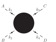
Figure 1: Meson-meson scattering process $A+B\to C+D$. with incoming momenta $k_{1}$, $k_{2}$ and outgoing momenta $k_{3}$, $k_{4}$. Dashed lines denote pseudoscalar mesons and the black dot their interaction.

We will analyze experimental/phenomenological data for the $\pi\pi$ and $K\pi$ scattering processes:

$$\pi\pi\to\pi\pi\,,\qquad\pi\pi\to K\overline{K}\,,\qquad K\pi\to K\pi\,.$$ (14)

The two-body kinematics (Fig. 1) is parametrized by the Mandelstam variables $s=\left(k_{1}+k_{2}\right)^{2}$, $t=\left(k_{1}-k_{3}\right)^{2}$ and $u=\left(k_{1}-k_{4}\right)^{2}$, with $\sqrt{s}$ the total energy in the center-of-mass (CM) system. In our case here, we consider a CM energy ranging from $\sqrt{s}=280$ MeV up to $\approx 1200$ MeV. At these energies the following additional channels are open:

$$\pi\pi\to\eta\eta\,,\qquad K\overline{K}\to\eta\eta\,,\qquad K\overline{K}\to K\overline{K}\,,$$

$$\eta\eta\to\eta\eta\,,\qquad K\eta\to K\pi\,.$$ (15)

Since in all processes the isospin and strangeness is conserved, one can write each scattering amplitude in terms of its contributions of total isospin $I$, with $I=0,\frac{1}{2},1,\frac{3}{2},2$ the only possible values here, and strangeness. Choosing $s$ and the scattering angle $\theta$ as the independent variables, each isospin-projected amplitude $T_{I}(s)$ can be further decomposed into its individual contributions with total angular momentum $J$ (for the sake of brevity, we will not make explicit reference to the strangeness quantum number):

$$T_{I}(s,t,u) = \sum_{J=0}^{\infty}\;\left(2J+1\right)\;T_{IJ}(s)\;P_{J}(\cos\theta)\,,$$ (16)

$$T_{IJ}(s) = \frac{1}{2N}\int_{-1}^{+1}d(\cos\theta)\;\,P_{J}(\cos\theta)\;T_{I}(s,t,u)\,$$ (17)

$$= -16\pi\;\frac{1}{2i\,\rho(s)}\;\left[\eta_{IJ}(s)\;e^{2i\delta_{IJ}(s)}-1\right],$$

with $P_{J}(x)$ the Legendre polynomials and $\rho(s)$ a channel dependent kinematical factor defined below, and $N$ is a normalization factor to account for identical particles, such that $N=2$ if all the particles in the process are identical and $N=1$ otherwise. Since we are working in the isospin limit, we consider the three pions as identical. Therefore, in our case, $N=2$ only for $\pi\pi\to\pi\pi$ and $\eta\eta\to\eta\eta$ processes. Explicitly, we analyze data for the three channels in Eq. (14) that come in terms of the scattering amplitudes $T_{IJ}(s)$, phase shifts $\delta_{IJ}(s)$ and inelasticities $\eta_{IJ}(s)$, defined in Eq. (17). To address the resonance properties, a unitarized framework is needed which leads to the inclusion of coupled channels at higher energies. Because of this, we need in addition to the above three channels also a theoretical description of the ones in Eq. (15). In that sense, the present work is an extension of Ref. Nieves:2011gb to more channels and higher scattering energies.

Meson-meson scattering within one-loop $\chi$PT was analyzed by Gómez-Nicola and Peláez in Ref. GomezNicola:2001as where, in addition, unitarization was implemented via the Inverse Amplitude Method (IAM). A naive addition of the missing LO contributions in $1/N_{c}$, within this scheme, would violate either unitarity or analyticity. We use here a scheme based on the Bethe-Salpeter equation (BSE) to restore two-body unitarity. The BSE on-shell scheme for the non-coupled channel was already described in Refs. Nieves:1999bx ; Nieves:1998hp for $\chi$PT and used in Nieves:2011gb when LO $1/N_{c}$ corrections were further included. The generalization to the coupled-channels situation needed here is straightforward. Let us consider the matrix $T_{IJ}(s)$ incorporating the partial-wave amplitudes of all relevant processes $AB\to CD$:

$$T_{IJ}(s)\;=\;\left[\begin{array}[]{ccc}T_{IJ}^{\pi\pi\to\pi\pi}(s)&T_{IJ}^{\pi\pi\to K\overline{K}}(s)&T_{IJ}^{\pi\pi\to\eta\eta}(s)\\ T_{IJ}^{K\overline{K}\to\pi\pi}(s)&T_{IJ}^{K\overline{K}\to K\overline{K}}(s)&T_{IJ}^{K\overline{K}\to\eta\eta}(s)\\ T_{IJ}^{\eta\eta\to\pi\pi}(s)&T_{IJ}^{\eta\eta\to K\overline{K}}(s)&T_{IJ}^{\eta\eta\to\eta\eta}(s)\end{array}\right]\,,$$ (18)

for the channels $\pi\pi\to\pi\pi$ and $\pi\pi\to K\overline{K}$, and

$$T_{IJ}(s)\;=\;\left[\begin{array}[]{cc}T_{IJ}^{K\pi\to K\pi}(s)&T_{IJ}^{K\pi\to K\eta}(s)\\[2.0pt] T_{IJ}^{K\eta\to K\pi}(s)&T_{IJ}^{K\eta\to K\eta}(s)\end{array}\right]\,,$$ (19)

for the channel $K\pi\to K\pi$. All $T_{IJ}^{AB\to CD}(s)$ are defined through Eq. (17), and the explicit form of the amplitudes $T_{I}\left(s,t,u\right)^{AB\to CD}$ is given in the Appendix A. Note that some of the above matrix elements are trivially zero from isospin or angular momentum conservation. For instance, in the $I=2$, $J=0$ channel, only $T_{IJ}^{\pi\pi\to\pi\pi}(s)$ is different from zero.

Coupled-channel unitarity is most simply expressed in terms of the inverse matrix $T_{IJ}^{-1}(s)$ as

$${\rm Im}T_{IJ}^{-1}(s)\;=\;-{\rm Im}\overline{\mathcal{I}}_{0}(s)\,,$$ (20)

where $\overline{\mathcal{I}}_{0}$ is a diagonal matrix of one-loop integrals characterizing the elastic two-body re-scattering:

$$\overline{\mathcal{I}}_{0}(s)\;=\;\mathrm{diag}\left[\overline{I}_{0}^{\pi\pi}(s),\,\overline{I}_{0}^{K\bar{K}}(s),\,\overline{I}_{0}^{\eta\eta}(s)\right]\,$$ (21)

or

$$\overline{\mathcal{I}}_{0}(s)\;=\;\mathrm{diag}\left[\overline{I}_{0}^{K\pi}(s)\,,\overline{I}_{0}^{K\eta}(s)\right]\$$ (22)

for the $\pi\pi$ and $K\pi$ cases, respectively. With two identical mesons,

$$\overline{\mathcal{I}}_{0}^{\phi\phi}(s)\;=\;\frac{1}{16\pi^{2}}\;\rho_{\phi}(s)\;\ln\left[\frac{\rho_{\phi}\left(s\right)+1}{\rho_{\phi}\left(s\right)-1}\right]\,,$$ (23)

where  $\rho_{\phi}(s)=\sqrt{1-4m_{\phi}^{2}/s}$  and

$${\rm Im}\overline{\mathcal{I}}_{0}^{\phi\phi}(s)\;=\;-\theta(s-4m_{\phi}^{2})\;\frac{1}{16\pi}\;\rho_{\phi}(s)\,.$$ (24)

The general expression in the case of two different mesons can be found in Eq. (A10) of Ref. Nieves:2001wt , identifying the function $L(s)$ that appears there to ${\mathcal{I}}_{0}^{\phi\phi^{\prime}}(s)/16\pi^{2}$. The definition/extension of the loop function to the SRS is given in Eq. (A13) of the same work.

We decompose the full $\chi$PT amplitude matrix $T_{IJ}^{\chi PT}\left(s\right)$ in its $\mathcal{O}(p^{2})$ and $\mathcal{O}(p^{4})$ contributions (in matrix notation):

$$T_{IJ}^{\chi PT}(s) \,= \,T_{IJ}^{\left(2\right)}(s)+T_{IJ}^{\left(4\right)}(s)+\mathcal{O}\left(p^{6}\right).$$ (25)

The coupled-channels unitarized amplitude is now written as:

$$T_{IJ}^{-1}\left(s\right)\;=\;V_{IJ}^{-1}(s)-\overline{\mathcal{I}}_{0}(s)-\mathcal{C}_{IJ}\,,$$ (26)

with $\mathcal{C}_{IJ}$ a diagonal matrix of subtraction constants:

$$\mathcal{C}_{IJ}\;=\;\mathrm{diag}\left[C_{IJ}^{\pi\pi},\,C_{IJ}^{K\bar{K}},\,C_{IJ}^{\eta\eta}\right]$$ (27)

or

$$\mathcal{C}_{IJ}\;=\;\mathrm{diag}\left[C_{IJ}^{K\pi},\,C_{IJ}^{K\eta}\right]\,.$$ (28)

The matrix $V_{IJ}(s)$ is defined such that a chiral expansion of $T_{IJ}(s)$ and $V_{IJ}(s)$ will match the one of $T_{IJ}^{\chi PT}(s)$. Inverting Eq. (26), we obtain the unitarized matrix $T_{IJ}(s)$:

$$T_{IJ}(s) = \left[V_{IJ}^{-1}(s)-\overline{\mathcal{I}}_{0}(s)-\mathcal{C}_{IJ}\right]^{-1}\,,$$ (29)

$$V_{IJ}(s) = T_{IJ}^{\chi PT}(s)-T_{IJ}^{\left(2\right)}\left[\overline{\mathcal{I}}_{0}(s)+\mathcal{C}_{IJ}\right]T_{IJ}^{\left(2\right)}.$$ (30)

Figure 2: Some ${\cal O}(p^{8})$ loop contributions generated when coupled-channels unitarity is restored (Eqs. (29), (30) and (31)). They give rise to pathologies when estimated using an on-shell approximation. In the bottom panel, the line shows a possible source of a physical imaginary part, when the particles cut by it are put on the mass shell.

As already noted in Ref. GomezNicola:2001as within the IAM method, the on-shell approximation in the coupled-channel potential has the drawback of generating spurious singularities below the opening of a new channel because the left-cut is analytically extrapolated below the inelastic threshold. For instance, as can be appreciated in the top panel of Fig. 2, for $\pi\pi\to\pi\pi$ below the $K\bar{K}$ threshold, the three loops $\pi\pi\to\bar{K}K\to\bar{K}K\to\pi\pi$ term contains in the on-shell $\bar{K}K\to\bar{K}K$ piece a $2\pi$-exchange contribution in the $t$ channel, generating a left-cut in the partial waves at $s=-4m_{\pi}^{2}+4m_{K}^{2}$ which sits in the elastic scattering region $4m_{\pi}^{2}<s<4m_{K}^{2}$. However, the effect is numerically quite small.

IV.1 $\mathcal{O}(p^{4})$ $\chi$PT  $\&$ single-resonance approximation (SRA) amplitudes and large$-N_{c}$ counting rules

To incorporate LO $1/N_{c}$ corrections in the description of the interactions among the Goldstone bosons, we follow the scheme derived in Nieves:2011gb . There, the leading-$N_{c}$ prediction for the actual $\pi\pi$ scattering amplitude was used as deduced from R$\chi$T, considering just the lowest-lying nonet of exchanged resonances Ecker:1988te ; Ecker:1989yg . Thus, let us denote by $T_{IJ}^{\rm SRA}(s)$, the two SU(3)-Goldstone-boson scattering amplitude within the SRA, obtained from the lowest-order R$\chi$T  Lagrangian Ecker:1988te ; Ecker:1989yg , and projected onto isospin and angular momentum. Below the resonance mass scale, the singularity associated with the pole of a resonance propagator could be replaced by the corresponding momentum expansion; therefore, the exchange of virtual resonances generates derivative Goldstone couplings proportional to powers of $1/m^{2}_{R}$. Let us denote by $T_{IJ}^{\rm(4)\,SRA}(s)$ the lowest-order term in derivatives. It gives the large-$N_{c}$ predictions for the $\mathcal{O}(p^{4})$ $\chi$PT  couplings Ecker:1988te ; Ecker:1989yg and constitutes the leading $1/N_{c}$ approximation to $T_{IJ}^{\chi PT}$. Our approach consists in using Eqs. (29) and (30), but replacing in the definition of the two particle irreducible amplitude $V_{IJ}(s)$, $T_{IJ}^{\chi PT}(s)$ by

$$T_{IJ}^{\chi PT}(s)\leftrightarrow\underbrace{T_{IJ}^{\rm SRA}(s)}_{{\cal O}(1/N_{c})}+\underbrace{\left(T_{IJ}^{\chi PT}(s)-T_{IJ}^{\rm(4)\,SRA}(s)\right)}_{{\cal O}(1/N^{2}_{c})}.$$ (31)

In this way, by construction, we recover the one-loop $\chi$PT  results, while at the same time all terms in the amplitude that scale like $1/N_{c}$ (leading) are also included within the SRA. Note that in the $1/N_{c}$ counting, the correction $\left(T_{IJ}^{\chi PT}(s)-T_{IJ}^{\rm(4)\,SRA}(s)\right)$ is incomplete, since it does not account for all existing subleading $1/N_{c}^{2}$ contributions to $T_{IJ}(s)$. A complete $1/N^{2}_{c}$ calculation would require quantum corrections stemming also from the low-lying resonances.

We should point out a problem that now appears when unitarity is restored. Let us pay attention for instance to the $\rho$-exchange, for $\pi\pi\to\pi\pi$ below the $K\bar{K}$ threshold. The $\pi\pi\to\bar{K}K\to\bar{K}K\to\pi\pi$ term contains a contribution from the intermediate $\bar{K}K\to\bar{K}K$ amplitude driven by $\rho$-exchange in the $t-$channel (see bottom panel of Fig. 2). Such contribution, within the on-shell scheme used here, leads to a spurious left-cut contribution at $s\leq 4m_{K}^{2}-m_{\rho}^{2}\sim(0.64~{}{\rm GeV})^{2}$, with very visible consequences if nothing is done. It is indeed unphysical, and it is an artifact of the on-shell unitarization in coupled channels adopted here. A contribution as the one described above can not physically give rise to an inelastic imaginary part below $s=(2m_{K}+m_{\rho})^{2}$, as trivially inferred from the optical theorem (see the shown cut in the figure). In our case we handle the problem by smoothly switching off coupled channels effects for $\sqrt{s}\leq 0.73$ GeV, and considering thus purely elastic $\pi\pi\to\pi\pi$ scattering below these energies, where coupled channel effects are expected to be negligible. The same procedure has been applied to other channels, where similar problems also show up. This problem appears but was not mentioned explicitly in Ref. Guo:2011pa and it was solved there by re-expanding the $\rho$-meson propagator as a polynomial, hence removing the singularity. Note that, the truncation of the expansion implies that in Guo:2011pa not all leading $1/N_{c}$ terms in the amplitude are included.

V Fitting strategies

V.1 Fitting parameters

Our 24 fitting parameters can be separated into partial-wave specific ones which play the role of renormalization constants,

$$C_{00}^{\pi\pi}\,,\,C_{11}^{\pi\pi}\,,\,C_{20}^{\pi\pi}\,,\,C_{00}^{K\bar{K}}\,,\,C_{00}^{\eta\eta}\,,\,C_{11}^{K\bar{K}}\,,$$

$$C_{\frac{1}{2}0}^{K\pi}\,,\,C_{\frac{1}{2}0}^{K\eta}\,,\,C_{\frac{1}{2}1}^{K\pi}\,,\,C_{\frac{1}{2}1}^{K\eta}\,,\,C_{\frac{3}{2}0}^{K\pi}\,,\,C_{\frac{3}{2}1}^{K\pi}\,,$$ (32)

and those which appear in the potential:

$$G_{V}\,,\,c_{d}\,,\,c_{m}\,,\,\tilde{c}_{d}\,,\,\tilde{c}_{m}\,,\,d_{m}\,,\,\tilde{d}_{m}\,,\,m_{S_{1}}\,,\,m_{S_{8}}\,,\,m_{V}\,,\,\mu_{V}\,,\,\mu_{S}\,.$$ (33)

The R$\chi$T predictions are supposed to be valid at some fixed value of the renormalization scale, which we allow to be different for vector ($\mu_{V}$) and scalar ($\mu_{S}$) couplings.

V.2 Fitted data and error assignment

An important novelty of this work is the use of the most precise and reliable output for the $\pi\pi$ and $\pi K$ scattering processes, which is a key factor to attaining high levels of precision and to fix the R$\chi$T parameters given in Eq. (33). In the $\pi\pi$ case, we use the recent data analysis given in GarciaMartin:2011cn . This analysis incorporates the latest data on $K_{l4}$ decays from NA48/2 Batley:2010zza as well as constraints from Roy equations and one-subtracted coupled dispersion relations - or GKPY (Garcia-Martin, Kaminski, Pelaez and Yndurain) equations. For the $\pi K$ case, we use the last update of the Roy-Steiner solutions in Buettiker:2003pp , which includes input from the $\pi K$ phase-shifts around 1.1 GeV and information on the vector $\pi K$ form-factor from tau decays. However, we do not fit to the $\delta^{\frac{3}{2}1}$ phase-shift, as this channel was not considered in the solution of the Roy-Steiner equations, and it came as prediction of the scheme. Thus, the subtraction constant $C_{\frac{3}{2}1}^{K\pi}$ in Eq. (V.1) cannot be determined.

In total, the data set which we are fitting is a compilation of 14 independent channels, shown in Table 2, from the above two independent sources. Additionally, despite using an elaborated theoretical model to describe these channels, we know that it contains systematic uncertainties (partial resummation) or neglected physics (isospin breaking). A key issue in our fit is therefore how to combine the different experimental and theoretical inputs in a consistent picture.

The first important point is the choice of the data errors for the individual channels. Unfortunately, for the $K\pi$ scattering, the output of the analysis in Ref. Buettiker:2003pp does not provide any errors. Nevertheless, the input contains some experimental uncertainties, typically of the 10% order, and we assume this to be the error for the $K\pi$-scattering data. The only exception is the $|T^{00}|$ case in $\pi\pi\to\bar{K}K$, for which due to its small value above 1 GeV, we also add 0.1 to the errors. In the case of the $\pi\pi$-scattering channels, we take the errors from the work of Ref. GarciaMartin:2011cn with two exceptions: the $\delta^{00}$ phase shift and the $\eta^{00}$ inelasticity. They are reported to be $1\sim 5$% and $\sim 20$%, respectively. Using these errors in a combined fit represents certain difficulties as they are very different compared to all the other channels or the assumptions that entered the model. On the one hand, the sharp error for the $\delta^{00}$ would drive the fit to precisely describe this channel on the expense of all the other ones, especially the $\eta^{00}$. On the other hand, we also do not expect our model to be accurate to a $<5$% level. Therefore, to have a more homogeneous error definition across all channels, we enlarge the reported $\delta^{00}$ error by a factor of $2$ and divide the reported $\eta^{00}$ errors by a factor of $2\sim 2.25$. The enlargement of the $\delta^{00}$ errors is thereby to be interpreted as a quantitative input of the model uncertainties to the fit. Concerning the reweighting of $\eta^{00}$, we hope that future, more precise data, will make this reweighting unnecessary. In addition, we will see later that the main results of this work are not significantly affected by this choice. Furthermore, our model does not include isospin breaking effects, which are known to play a crucial role in the $\delta^{00}$ channel of $\pi\pi\to\pi\pi$ around the region $990$ MeV $<\sqrt{s}$ $<1010$ MeV. We therefore exclude these data points from the fit.

The second important issue is connected to the used pseudo data points as their number in each channel is arbitrary. They are analytically generated from the theoretical analyses carried out in Refs. GarciaMartin:2011cn ; Buettiker:2003pp , usually in intervals of $5$ MeV. To reduce the dependence on this, we normalize each contribution from a given channel by the number of data points in that channel. The exact $\chi^{2}$ definition is given in the next section. In using this normalized approach, the reduction of the $\eta^{00}$ errors by $2\sim 2.25$ is equivalent to give an extra weight of $4\sim 5$ to this channel in the overall $\chi^{2}$.

With the above settings we will be able to obtain a consistent fit that homogeneously describes all the 14 channels as well as is compatible with the theoretical assumptions entering the model.

dataset	range (GeV)	errors			$\chi^{\prime 2}$
$\pi\pi\to\pi\pi$  GarciaMartin:2011cn
$\delta^{00}$	[0.28,1.2]	(*)			1.6
$\delta^{11}$	[0.28,1.2]				1.0
$\delta^{20}$	[0.28,1.2]				0.7
$\eta^{00}$	[0.28,1.2]	(**)			0.5
$\eta^{11}$	[0.28,1.2]				0.0
$\pi\pi\to K\bar{K}$  Buettiker:2003pp
$|T^{00}|$	[0.99,1.2]	10%			0.8
$\delta^{00}$	[0.99,1.2]	$10\%$			0.2
$|T^{11}|$	[0.99,1.2]	10%			0.1
$\delta^{11}$	[0.99,1.2]	10%			0.0
$\pi K\to\pi K$  Buettiker:2003pp
$\delta^{\frac{1}{2}0}$	[0.64,1.2]	$10\%$			1.2
$\delta^{\frac{1}{2}1}$	[0.64,1.2]	$10\%$			0.8
$\delta^{\frac{3}{2}0}$	[0.64,1.2]	$10\%$			0.4
$\eta^{\frac{1}{2}0}$	[0.64,1.2]	0.05			0.0
$\eta^{\frac{1}{2}1}$	[0.64,1.2]	0.05			0.0

Table 2: Compilation of data included in the fit. In the case of the $\pi\pi\to\pi\pi$ channels we take the errors as obtained from the CFD parametrization derived in GarciaMartin:2011cn , with two exceptions: in (*) the errors have been multiply by a factor 2 and the region between $990\,{\rm MeV}\,<\sqrt{s}<1010$ MeV has been excluded from the fit, in (**) the errors have been reduced by a factor of $2.25$ (see text for details). The errors on the $\pi\pi\to K\bar{K}$ and $\pi K\to\pi K$ data-sets have been obtained from the experimental input uncertainties in Buettiker:2003pp (see Figs. 2, 4, 8 and 9 of this reference), however, in the case of $|T^{00}|$ we also added an absolute 0.1 error above 1 GeV. In the last column, we show the contribution $\chi^{2}_{\rm chan}$ of each channel as defined in Eq. (35).

V.3 The usual $\chi^{2}$ approach

On the one hand, a fit to the scattering data of the $N_{dc}=14$ channels involves the standard $\chi^{2}$, defined as

$$\chi^{2}_{\rm exp} = N_{d}\sum_{\rm chan=1}^{N_{dc}}\chi^{2}_{\rm chan}\;\;\;,$$ (34)

$$\chi^{2}_{\rm chan} = \frac{1}{n}\sum_{i=1}^{n}\;\left(\frac{O_{i}^{\rm th}-O_{i}^{\rm exp}}{\Delta O_{i}^{\rm exp}}\right)^{2}\,,$$ (35)

$N_{d}$ the overall total number of data points. The $(O_{i}^{\rm exp},\Delta O_{i}^{\rm exp})$ are the fitted observables with their corresponding errors, and $O_{i}^{\rm th}=F_{i}(p,C)$ are our theoretical descriptions, with $p_{j}=G_{V},c_{d},\dots$ parameters subjected to theoretical conditions and $C_{j}=C_{00}^{\pi},\dots$ parameters which can only be determined from data. On the other hand, we typically expect our calculation to be accurate up to $1/N_{c}$ corrections. Thus, if a fit turns out to provide numbers completely different from the large-$N_{c}$ estimates of Eqs. (8) and (9), we will suspect the fit. The optimal situation would be when the data would have an accuracy able to pin down reliably all the parameters. Unfortunately, this is not the case. Attempts to determine the $C_{IJ}$ subtraction constants in Eq. (V.1) and the R$\chi$T parameters in Eq. (33) (in all 23 parameters) produce multiple minima with at times quite unreasonable values for the R$\chi$T parameters. In this case, we are inclined to reject the fit. If, on the other hand, the large-$N_{c}$ constraints are fully implemented and larger error bands are assumed, the resulting fits are likewise not satisfactory.

We want to obtain a reasonable fit with sensible parameters. Therefore, rather than expecting the fit to tell us a posteriori whether the parameters are reasonable, we provide a priori a reasonable guess for the parameters and search for the minimum within the expected departure of this assumption. In the next section, we explain how we include the a priori input in the fit.

The existence of multiple solutions is a consequence of several shallow directions in the parameter space, which it makes impossible to identify a unique global minimum. This situation could be solved by including further experimental or theoretical information. For example, data of those channels that, considered in the coupled channel formalism, have not been fitted. Unfortunately, this is not the case, and a Bayesian fit with large-$N_{c}$ priors becomes a natural and simple way to circumvent this problem.

Guo and Oller Guo:2011pa handle the problem of proliferation of parameters in a different manner. They took free values for all the resonance parameters ($p_{j}$ in our notation) but they invoked to some unclear SU(3) relations among the subtraction constants ($C_{j}$ in our notation), and kept just four independent. However, this is not a consistent approach. First, the subtraction constants are not in principle related by SU(3) and should all be taken as independent (see discussion in Nieves:1999bx ). Second, the unconstrained fit of the resonance parameters to data led in some cases to values in clear contradiction to the large-$N_{c}$ expectations. Conversely, the Bayesian approach to be discussed below, where large $N_{c}$ constraints are imposed as a probabilistic prior, does not support the assumptions of Ref. Guo:2011pa .

V.4 The augmented $\chi^{2}$ approach

In the Bayesian interpretation, the fitting parameters are actually random variables which are determined from the existing given data and a prior probability of finding the parameters, regardless of the actual measurements under analysis. We shall not dwell into the philosophical intricacies and use the augmented $\chi^{2}$ method to fix the prior distribution Lepage:2001ym ; Morningstar:2001je ; Schindler:2008fh . This approach has successfully been used in lattice QCD to analyze a number of data with a similar number of parameters. In our case the situation is slightly different, but we expect the large-$N_{c}$ limit to set reasonable ranges on the fitting parameters.

We consider first the theoretical $\chi^{2}$ defined in Eq. (13). This figure of merit is coherent with the assumption that the prior probability for the R$\chi$T parameters is given by their large-$N_{c}$ estimate, within a relative $1/N_{c}$ accuracy (and not as an uniform distribution). We use the results of Eq. (8) for $G_{V},\tilde{c}_{m},c_{d},\tilde{c}_{d},d_{m},\tilde{d}_{m}$ and Eq. (9) for $m_{S_{0}},m_{S_{8}},m_{V}$. Thus, we take the following Gaussian variables normalized to the same $\Delta p_{i}=f_{\pi}/N_{c}$:

$$\xi_{G_{V}} \!\!= \!\!\frac{\sqrt{2}G_{V}-f_{\pi}}{f_{\pi}/N_{c}}\,,\qquad\xi_{c_{d}}\,=\,\frac{2c_{d}-f_{\pi}}{f_{\pi}/N_{c}}\,,\qquad\dots$$

$$\xi_{m_{V}} \!\!= \!\!\frac{\sqrt{N_{c}/24\pi^{2}}m_{V}-f_{\pi}}{f_{\pi}/N_{c}}\,,\qquad\dots$$ (36)

We provide in addition an a priori splitting $m_{S_{0}}-m_{S_{8}}$ for the scalar octet and singlet masses, which are equal at large $N_{c}$:

$$\xi_{m_{S_{0}}-m_{S_{8}}}\;=\;\sqrt{\frac{N_{c}}{24\pi^{2}}}\;\frac{m_{S_{0}}-m_{S_{8}}}{f_{\pi}/N_{c}}\,,$$ (37)

and we finally also consider the robust constraint in the large $N_{c}$ limit $4c_{d}c_{m}\sim f_{\pi}^{2}$, obtained by requiring the $K\pi$ scalar form factor to vanish in the $t\to\infty$ limit Jamin:2000wn ,

$$\xi_{c_{d}c_{m}}=\frac{\sqrt{4c_{d}c_{m}}-f_{\pi}}{f_{\pi}/N_{c}}\,.$$ (38)

Thus, we take into account a total of 10 contributions to construct $\chi^{2}_{\rm th}$,

$$\chi^{2}_{\rm th} = \left[\xi_{G_{V}}^{2}+\xi_{c_{d}}^{2}+\xi^{2}_{c_{d}c_{m}}+\xi_{d_{m}}^{2}+\xi^{2}_{\tilde{c}_{d}}+\xi^{2}_{\tilde{c}_{m}}+\xi_{\tilde{d}_{m}}^{2}\right]$$ (39)

$$+ \left[\xi_{m_{V}}^{2}+\xi_{m_{S_{8}}}^{2}+\xi_{m_{S_{0}}-m_{S_{8}}}^{2}\right].$$

In addition, we take for the singlet and octet pseudoscalar resonance masses $m_{P_{i}}=\sqrt{2}m_{S_{i}},\,i=0,8$, see section II.

The key question now is how to combine $\chi^{2}_{\rm exp}$ and $\chi^{2}_{\rm th}$. Obviously, since we have a small number of constraints $N_{p}$ as compared to the number of data or pseudo-data $N_{d}$, a direct addition of $\chi^{2}_{\rm exp}$ and $\chi^{2}_{\rm th}$ would make the constraints irrelevant. Therefore we will construct a reduced $\chi^{2}$, $\bar{\chi}^{2}\equiv\chi^{2}/N$, with a $50\%$ weighting on the data/pseudo-data and the theoretical constraints.

Thus, we define

$$\chi^{2}_{\rm total}\;=\;\frac{N_{d}+N_{p}}{2}\;\left(\frac{\chi^{2}_{\rm exp}}{N_{d}N_{dc}}+\frac{\chi^{2}_{\rm th}}{N_{p}}\right)\,.$$ (40)

The additional terms in the total $\chi^{2}$ impose a penalty for fits which deviate from the large-$N_{c}$ expectations by more than $1/N_{c}$. This is just a condition on the naturalness of parameters, based on a simple large-$N_{c}$ estimate. Of course, the values we are taking as a reference are based just on the single-resonance approximation, and this is precisely why one should not attach exaggerated significance to the detailed accuracy of the reasonable fit. The opposite situation, the impossibility of performing a successful fit would signal a serious drawback of the whole framework, including the usefulness of the short-distance constraints in meson-meson scattering.

Furthermore, we have checked our approach against the weighting choice of Eq. (40). We found that the parameters in Table 3 do not depend strongly on this particular setting as long as the fit starts in the vicinity of the respective minimum. That is, the augmentation of Eq. (40) is needed to isolate the physical minimum of Table 3 from all the unphysical local minima, but after having found it the corresponding parameters do not strongly depend on the specific choice of Eq. (40).

V.5 Results

Parameter	Large $N_{c}$	Fit			Fit
$G_{V}$	$65.3$	$63.2\,(1)$		$C_{00}^{\pi\pi}$	$-0.0209\,(2)$
$c_{d}$	$46.2$	$39.8\,(1)$		$C_{00}^{K\bar{K}}$	$-0.0085\,(3)$
$\tilde{c}_{d}$	$26.7$	$20.7\,(3)$		$C_{00}^{\eta\eta}$	$0.0060\,(2)$
$c_{m}$	$46.2$	$41.1\,(1)$		$C_{11}^{\pi\pi}$	$-0.0279\,(6)$
$\tilde{c}_{m}$	$26.7$	$18.9\,(9)$		$C_{11}^{K\bar{K}}$	$-0.0100\,(5)$
$d_{m}$	$32.7$	$29.8\,(1)$		$C_{20}^{\pi\pi}$	$-0.0561\,(5)$
$\tilde{d}_{m}$	$18.9$	$19.3\,(7)$		$C_{\frac{1}{2}0}^{K\pi}$	$-0.0029\,(3)$
$m_{V}$	$821$	$805\,(2)$		$C_{\frac{1}{2}0}^{K\eta}$	$-0.0165\,(14)$
$m_{S_{0}}$	$821.0$	$808.9\,(4)$		$C_{\frac{1}{2}1}^{K\pi}$	$0.0380\,(20)$
$m_{S_{8}}$	$821$	$1279\,(9)$		$C_{\frac{1}{2}1}^{K\eta}$	$-0.0240\,(20)$
$\mu_{V}$		$645\,(4)$		$C_{\frac{3}{2}0}^{K\pi}$	$-0.0394\,(14)$
$\mu_{S}$		$274\,(10)$		$C_{\frac{3}{2}1}^{K\pi}$	$-$

Table 3: Parameters (in MeV) of the R$\chi$T Lagrangian determined from phenomenology Ecker:1988te ; Ecker:1989yg or short-distance constraints Pich:2002xy and the resulting values from the combined fit. Resonance masses and saturation scales are also given in MeV, while subtraction constants are dimensionless.

$I$	$J$		$\sqrt{s_{R}}$ [MeV]	$|g_{\pi\pi,\pi K}|$ [GeV]	$|g_{\bar{K}K}|$ [GeV]	PDG  Beringer:1900zz $\sqrt{s_{R}}$ [MeV]	GKPY/RS GarciaMartin:2011jx ; DescotesGenon:2006uk $\sqrt{s_{R}}$ [MeV]
0	0	$f_{0}(500)$ or $\sigma$	$458(2)-i\,264(3)$	$3.3(1)$	$0.9(1)$	$400\sim 550-i\,[200\sim 350]$	$457^{+14}_{-13}-i\,279^{+11}_{-7}$
0	0	$f_{0}(980)$	$1001(4)-i\,24(2)$	$2.2(1)$	$4.2(1)$	$990\pm 20-i\,[20\sim 50]$	$996(7)-i\,25^{+10}_{-6}$
0	0		$1211(64)-i\,332(78)$	$3.3(5)$	$2.6(2)$
0	0		$1449(29)-i\,61(12)$	$3.1(2)$	$0.3(1)$
1	1	$\rho(770)$	$761(3)-i\,73(2)$	$6.0(1)$	$3.9(1)$	$772.3(9)-i\,75.1(8)^{*}$	$763.7^{+1.7}_{-1.5}-i\,73.2^{+1.0}_{-1.1}$
$1/2$	0	$K_{0}^{*}(800)$ or $\kappa$	$684(4)-i\,260(4)$	$4.2(1)$		$682(29)-i\,273(12)$	$659(13)-i\,278(12)$
$1/2$	1	$K^{*}(892)$	$897(5)-i\,24(2)$	$5.4(3)$		$896.1(19)-i\,23.7(3)^{*}$

Table 4: Pole positions and resonance couplings found in this work with the best fit parameters compiled in Table 3. All statistical uncertainties are defined on a 68% confidence-level. For the resonances marked with $(^{*})$, the PDG quote Breit-Wigner (BW) parameters $s_{\rm pole}=M_{BW}^{2}-iM_{BW}\Gamma_{BW}$, from which we have computed the corresponding pole positions. For the $\rho(770)$ case we show the “Neutral only, other reactions” average values, whereas for the $K^{*}(892)$ we give the “Neutral only” average mass and width. Note that the dispersive data analysis of Ref. Caprini:2005zr , based in the Roy equations, predict $\sqrt{s_{\sigma}}=(441^{+16}_{-8}-i\,272^{+9}_{-12})$ MeV. In addition, the $|g_{\pi\pi}|$ GKPY dispersive determination given in GarciaMartin:2011jx for the $f_{0}(500)$, $f_{0}(980)$ and $\rho(770)$ are $3.59^{+0.11}_{-0.13}$, $2.3\pm 0.2$ and $6.01^{+0.04}_{-0.07}$ respectively.

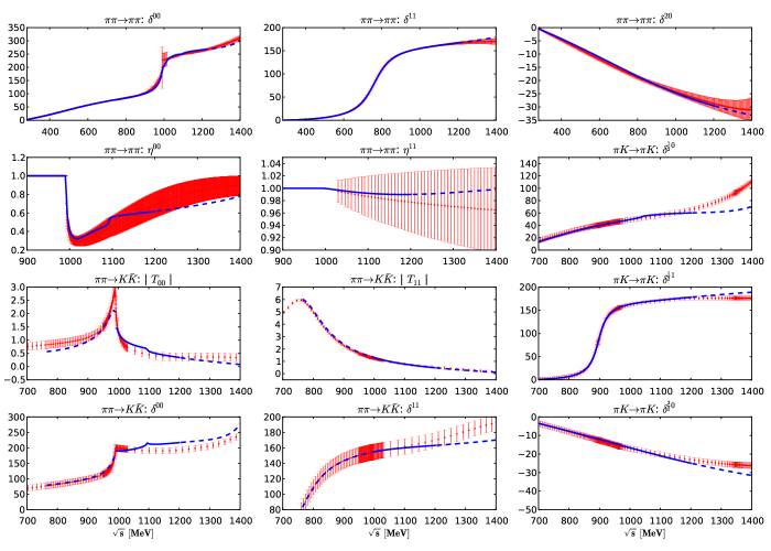
Figure 3: Results for meson-meson scattering observables as a function of the CM energy $\sqrt{s}$ (in MeV). We display the pseudo-data, with their assumed uncertainties, included in the fit (see Table 2). Solid lines represent fitted curves, dashed (blue) lines represent non-fitted curves.

The values of the fitted parameters are presented in Table 3 and the results for scattering properties are depicted in Fig. 3, where solid (blue) lines represent fitted curves. The results for non-fitted data are depicted as dashed (blue) lines. In the Bayesian approach, errors on the parameters are estimated as mean values, i.e., integrating the likelihood with respect to the fitting parameters, but when the total $\chi^{2}$ is large (not the $\chi^{2}/{\rm d.o.f.})$, as it is the case here, a saddle point approximation can be used. This is just equivalent to determine them by the standard covariance matrix inversion method applied in our case to Eq. (40).

As expected, the fit below $\Lambda_{R}=1.2$ GeV is successful with reasonable resonance parameters motivated by large-$N_{c}$ constraints (when states with mass above $\Lambda_{R}$ are disregarded). Indeed, as it can be seen in the Table 3, all R$\chi$T  parameters turn out to be in agreement, within the typical 30% uncertainty, with the large-$N_{c}$ expectations. The only exception is the value of $m_{S_{8}}\sim 1280$ MeV, which lies outside of the $N_{c}$ expected region. However, the mean between the two scalar masses, $m_{S_{8}}$ and $m_{S_{0}}$, satisfies this constraint.

The achieved description for all considered 14 pseudo-data channels is quite good, as can be appreciated in Fig. 3. This is even more relevant, taking into account that the comparison is being made with the quite precise output obtained from the data constrained Roy-GKPY and Roy-Steiner analyses carried out in Refs. GarciaMartin:2011cn ; Buettiker:2003pp , which provide the most reliable information currently available in the literature on the various scattering amplitudes.

Next, we discuss the poles found in the SRS of the amplitudes. The SRS of the $T$ matrix is determined by the definition of the loop function ${\mathcal{I}}_{0}^{\phi\phi^{\prime}}(s)$. As mentioned above, we use the Eq. (A13) of Ref. Nieves:2001wt . Masses and widths of the dynamically generated resonances are determined from the positions of the poles, $s_{R}$, in the SRS of the corresponding scattering amplitudes in the complex $s$ plane. Since in the SRA amplitudes we have explicitly incorporated one vector and two scalar poles, we expect at least these poles to appear in the appropriate sectors. However, because of the re-summation in Eq. (29), the pole positions will change with respect to those of the bare ones ($s=m^{2}_{V},m^{2}_{S_{0}}$ and $m^{2}_{S_{8}}$) and the resonances will acquire a width that accounts for their two-meson decay. This change is specially relevant for the $f_{0}(500)$ or $\sigma$ meson, where pion loops dominate at $N_{c}=3$, producing a state very deep on the complex plane, with a mass around 450 MeV and a width around 520 MeV. As studied in Cohen:2014vta , this effect is due to a strong cancellation between different $N_{c}$ orders, which makes it difficult to analyze its properties just from the pure $1/N_{c}$ expansion. In fact, there are several works in the literature Nieves:2011gb ; Pelaez:2003dy ; RuizdeElvira:2010cs ; Guo:2011pa ; Guo:2012yt ; Guo:2012ym , in which the $f_{0}(500)$ fades away on the complex plane as $N_{c}$ increases, being made just of meson-meson loops, and having then, no relation with the scalar poles included in the Lagrangian.

In addition, as we will see, some other poles are generated as well in the SRS of the scattering amplitudes. The results are presented in the Table 4. We find a quite good description of the $f_{0}(500),f_{0}(980),K^{*}_{0}(800),\rho(770)$ and $K^{*}(892)$ resonances, with masses and widths that compare rather well with the averaged ones compiled in the Review of Particle Properties Beringer:1900zz . Furthermore, since our results have been obtained by fitting the pseudo-data values obtained in the $\pi\pi$ GarciaMartin:2011cn and $\pi K$ Buettiker:2003pp dispersive analyses, we also include in the last row of Table 4, the dispersive determinations obtained from these schemes GarciaMartin:2011jx ; DescotesGenon:2006uk . The agreement is also remarkable. We want to note that the properties of all these dynamically generated states are not significantly affected by the employed re-weighting of the $\delta^{00}$ and $\eta^{00}$ channels.

Let us now pay attention to the complex pole structure of the scalar-isoscalar sector, depicted in Fig. 4. The $f_{0}(500)$ and $f_{0}(980)$ resonances are clearly visible. Besides, there appear two additional poles, which are placed above $\Lambda_{R}=1.2$ GeV. Perhaps, the lower one could have some relation with the $f_{0}(1370)$ state. This will agree with the findings of Ref. Albaladejo:2008qa , where the $f_{0}(1370)$ is identified as a pure octet state not mixed with the glueball. The chiral unitary approaches, supplemented by the inclusion of vector mesons, of Refs. Geng:2008gx ; GarciaRecio:2010ki ; Garcia-Recio:2013uva seem to give also support to this hypothesis. Nevertheless, the exact position of the higher poles depends much more on the choice of the merit function which is being minimized. Especially, the position of the $f_{0}(1370)$ depends strongly on how the comparatively imprecise $\eta^{00}$ pseudo data is included in the fit. In addition, these states are located above the scale of the first resonance multiplet considered, and then, are strongly dependent on those heavier states integrated out in the starting Lagrangian. Therefore, these heavier poles cannot be properly described within the framework used in this work and are included only for completeness.

Finally in Table 4, we also provide for each resonance its coupling to the fitted channels, ($\pi K$ in the case of the $K^{*}_{0}(800)$ and $K^{*}(892)$, and $\pi\pi$ and $KK$ for the others), defined from its pole residue as,

$$g_{A}g_{B}=\lim_{s\rightarrow s_{\rm pole}}(s-s_{\rm pole})T_{IJ}^{A\to B}(s)(2J+1)/(2p)^{2J},$$ (41)

where $p$ is the center-of-mass-system momentum of the corresponding process.

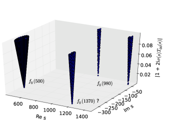
Figure 4: Poles found in the SRS of scalar-isoscalar elastic $\pi\pi$ amplitude. The $f_{0}(500)$ and $f_{0}(980)$ are clearly visible.

VI Conclusions

Within a unitarized coupled-channel approach, we have analyzed the scattering of the pseudo-scalar mesons for $\sqrt{s}\leq 1.2$ GeV, where all two-body scattering channels are open. Our amplitudes contain one-loop (NLO) $\chi$PT and tree-level (LO) large-$N_{c}$ pieces, with 24 fitting parameters. Given the lack of very precise experimental data, in this work we have used the most precise and reliable output for the $\pi\pi$ and $\pi K$ scattering processes from the Roy-GKPY and Roy-Steiner analyses carried out in Refs. GarciaMartin:2011cn ; Buettiker:2003pp . This is a major novelty of this work, since for the very first time, these two sets of data or pseudo-data have been simultaneously used to constrain the LECs. Indeed, it has been a key factor to attaining high levels of precision and to fix the R$\chi$T parameters. However, not all of the pseudo-data have experimentally inherited uncertainties, and hence an educated guess in defining the used merit function has been made.

While our model contains important features of the true solution and we optimized it by minimizing the discrepancies with experiment, the large number of best fit parameters made the task of performing the fit difficult. We faced a quite complex structure of the parameters manifold, which has many resemblances to a multidimensional egg-box. The proliferation of undetermined LECs made direct fits rather elusive and quite often we were driven to unreasonable parameter values, which suggested rejecting the fit. Under these circumstances, we have adopted the Bayesian point of view of making the natural assumption that the R$\chi$T parameters take their large-$N_{c}$ estimated values within an expected $1/N_{c}$ uncertainty.

The main outcome of the present study is that a rather good description of the data can be achieved with natural values of the parameters and considering the nominal expected accuracy of the calculations. This is a non-trivial result, and an important ingredient for this success is the allowance for systematic deviations in all parameters where the large-$N_{c}$ expansion is expected to provide corrections of ${\cal O}(1/N_{c})$. The predictions compiled in Table 4 for pole positions and couplings of the lowest-lying dynamically generated resonances, which show a nice agreement with the most precise current determinations, are an example of this success.

Appendix A SRA R$\chi$T  and one-loop $\chi$PT  amplitudes

The ${\cal O}(p^{4})$ $\chi$PT  amplitudes ($T_{IJ}^{\chi PT}(s)$) used through this work are obtained from Ref. GomezNicola:2001as . There, and assuming crossing symmetry, the isospin projected amplitudes for every possible process involving $\pi,K,\eta$ mesons can be found. Next, the individual contributions with total angular momentum $J$ are calculated using Eq. (17). Possible $\eta-\eta^{\prime}$ mixing effects are not taken into account, and thus the $\eta$ meson is identified with the isospin singlet ($\eta_{8}$) of the octet of Goldstone bosons. In addition, the normalizations used here are such that our amplitudes differ in one sign with those given in GomezNicola:2001as .

• $\pi\pi\to\pi\pi$: There is only one independent amplitude, $T(s,t,u)$, that is taken to be the $\pi^{+}\pi^{-}\to\pi^{0}\pi^{0}$, which at one loop in $\chi$PT  is given in Eq. (B4) of Ref. GomezNicola:2001as . Linear combinations of $T(s,t,u)$, $T(t,s,u)$ and $T(u,t,s)$ provide the isoscalar, isovector and isotensor amplitudes (see text above Eq.(12) in GomezNicola:2001as ).

• $K\pi\to K\pi$: Crossing symmetry allows us to write the $I=1/2$ amplitude (Eq.(12) in GomezNicola:2001as ) in terms of the $I=3/2$ $K^{+}\pi^{+}\to K^{+}\pi^{+}$ one, which is given in Eq. (B5) of Ref. GomezNicola:2001as .

• $K\bar{K}\to K\bar{K}$: In this case, the two isospin amplitudes can be expressed in terms of the $\bar{K}^{0}K^{0}\to K^{+}K^{-}$ amplitude (see Eq. (25) of Ref. Guo:2011pa ), which expression to one loop can be obtained from Eq. (B8) of GomezNicola:2001as . Note that this latter equation suffers from a typo and there, it turns out to be the amplitude $K^{0}\bar{K}^{0}\to K^{+}K^{-}$ the one which is given instead of the $\bar{K}^{0}K^{0}\to K^{+}K^{-}$ one.

• $K\bar{K}\to\pi\pi$: Thanks to crossing symmetry, the amplitudes in this sector are determined by the $I=3/2$ $K^{+}\pi^{+}\to K^{+}\pi^{+}$ one.

• $K\eta\to K\eta$: This is a pure $I=1/2$ process. The one-loop amplitude is given in Eq. (B2) of Ref. GomezNicola:2001as .

• $\bar{K}K\to\eta\eta$: This is an $I=0$ process that using crossing symmetry can be obtained from the previous amplitude.

• $K\eta\to K\pi$: This is also an $I=1/2$ process, and the one loop expression for $\bar{K}^{0}\eta\to K^{0}\pi^{0}$ can be found in Eq. (B3) of Ref. GomezNicola:2001as .

• $KK\to\pi\eta$: This $I=1$ process is related to the $\bar{K}^{0}\eta\to K^{0}\pi^{0}$ amplitude by crossing symmetry.

• $\pi\eta\to\pi\eta$: This is a pure $I=1$ isospin process, and its amplitude is given in Eq. (B6) of Ref. GomezNicola:2001as .

• $\pi\pi\to\eta\eta$: This amplitude is determined from the previous one by crossing.

• $\eta\eta\to\eta\eta$: This pure $I=0$ amplitude at one loop in $\chi$PT  is given in Eq. (B1) of Ref. GomezNicola:2001as .

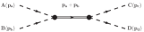
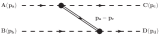
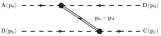
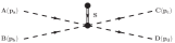
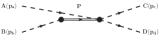
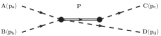
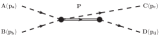
Figure 5: Resonance contributions to the pseudo-scalar meson-meson scattering . The dotted lines denote pseudo-scalar mesons, double lines the intermediate resonances and the black dot their interaction. The first row contains the diagrams with intermediate vector and scalar resonances in the $s$, $t$ and $u$ channel graphs. The pseudo-scalar resonances contributions are shown in the second row.

Next, we compile the R$\chi$T  amplitudes $T^{\rm SRA}(s,t,u)$, within the SRA, for the independent processes mentioned above. The different Feynman diagrams corresponding to the resonance exchange amplitudes are illustrated in Fig. 5. Note that, as it has been anticipated in Eq. (31), tree level amplitudes are also included in $T^{\rm SRA}(s,t,u)$. In addition, resonances also contribute indirectly through the diagrams of Fig. 6 which modify at $\mathcal{O}\left(p^{4}\right)$ the pion-decay constant and the pseudo-scalar meson self-energy $\Sigma^{R}_{\phi=\pi,K,\eta}(p^{2})$, and consequently, pseudo-scalar masses and wave-function renormalization constants. The scalar and pseudo-scalar resonances contribution to the pion-decay constant and self energy renormalization reads,

$$f_{\pi} = f\left(1+\frac{8}{3}\frac{c_{m}c_{d}}{f_{0}^{2}m_{S_{8}}^{2}}\left(m_{\pi}^{2}-m_{K}^{2}\right)+4\frac{\tilde{c}_{m}\tilde{c}_{d}}{f_{0}^{2}m_{S_{0}}^{2}}\left(2m_{K}^{2}+m_{\pi}^{2}\right)\right),$$

$$\Sigma_{\pi}^{S}\left(p^{2}\right) = \frac{-16c_{m}\left(m_{\pi}^{2}-m_{K}^{2}\right)}{3f_{0}^{2}m_{S_{8}}^{2}}\left[c_{d}p^{2}-c_{m}m_{\pi}^{2}\right]-\frac{8\tilde{c}_{m}\left(2m_{K}^{2}+m_{\pi}^{2}\right)}{f_{0}^{2}m_{S_{0}}^{2}}\left[\tilde{c}_{d}p^{2}-\tilde{c}_{m}m_{\pi}^{2}\right],$$

$$\Sigma_{K}^{S}\left(p^{2}\right) = \frac{-8c_{m}\left(m_{\pi}^{2}-m_{K}^{2}\right)}{3f_{0}^{2}m_{S_{8}}^{2}}\left[-c_{d}p^{2}+c_{m}m_{K}^{2}\right]-\frac{8\tilde{c}_{m}\left(2m_{K}^{2}+m_{\pi}^{2}\right)}{f_{0}^{2}m_{S_{0}}^{2}}\left[\tilde{c}_{d}p^{2}-\tilde{c}_{m}m_{K}^{2}\right],$$ (42)

$$\Sigma_{\phi=\pi,K}^{P}\left(p^{2}\right) = 8\frac{d_{m}^{2}m_{\phi}^{4}}{f_{0}^{2}}\frac{1}{p^{2}-m_{P_{8}}^{2}},$$

$$\Sigma_{\eta}^{S}\left(p^{2}\right) = \frac{4}{3}\Sigma_{K}^{S}\left(p^{2}\right)-\frac{1}{3}\Sigma_{\pi}^{S}\left(p^{2}\right).$$

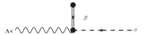
Figure 6: Scalar and pseudo-scalar resonance contributions to the pseudo-scalar meson self-energy and scalar one to the pion decay constant $f_{\pi}$.

Therefore, taking into account all these contributions, the $T^{\rm SRA}(s,t,u)$ amplitude for the channel $\pi^{+}\pi^{-}\to\pi^{0}\pi^{0}$ is given by:

$$T^{\rm SRA}(s,t,u) = \frac{1}{f_{\pi}^{2}}\left(m_{\pi}^{2}-s\right)+\frac{G_{V}^{2}}{f_{\pi}^{4}}\left(\frac{t\left(s-u\right)}{t-m_{V}^{2}}+\frac{u\left(s-t\right)}{u-m_{V}^{2}}\right)+\frac{2\left(2c_{m}m_{\pi}^{2}+c_{d}\left(-2m_{\pi}^{2}+s\right)\right)^{2}}{3f_{\pi}^{4}\left(s-m_{S_{8}}^{2}\right)}$$ (43)

$$+\frac{4\left(2\tilde{c}_{m}m_{\pi}^{2}+\tilde{c}_{d}\left(-2m_{\pi}^{2}+s\right)\right)^{2}}{f_{\pi}^{4}\left(s-m_{S_{0}}^{2}\right)}-\frac{8m_{\pi}^{4}d_{m}^{2}}{f_{\pi}^{4}\left(m_{\pi}^{2}-m_{P_{8}}^{2}\right)}.$$

For the channel $K^{+}\pi^{+}\to K^{+}\pi^{+}$,

$$T^{\rm SRA}(s,t,u) = \frac{1}{2f_{\pi}^{2}}\left(s-m_{K}^{2}-m_{\pi}^{2}\right)-\frac{G_{V}^{2}}{2f_{\pi}^{4}}\left\{\frac{t(s-u)}{t-m_{V}^{2}}+\frac{\left(t-2m_{K}^{2}\right)\left(t-2m_{\pi}^{2}\right)-(m_{K}^{2}+m_{\pi}^{2}-s)^{2}}{u-m_{V}^{2}}\right\}$$

$$+\frac{4\left(2(-\tilde{c}_{d}+\tilde{c}_{m})m_{K}^{2}+\tilde{c}_{d}t\right)\left(2(-\tilde{c}_{d}+\tilde{c}_{m})m_{\pi}^{2}+\tilde{c}_{d}t\right)}{f_{\pi}^{4}\left(t-m_{S_{0}}^{2}\right)}+\frac{\left((c_{d}-c_{m})\left(m_{K}^{2}+m_{\pi}^{2}\right)-c_{d}u\right)^{2}}{f_{\pi}^{4}\left(u-m_{S_{8}}^{2}\right)}$$

$$-\frac{\left(2(c_{d}-c_{m})m_{K}^{2}-c_{d}t\right)\left(2(c_{d}-c_{m})m_{\pi}^{2}-c_{d}t\right)}{3f_{\pi}^{4}\left(t-m_{S_{8}}^{2}\right)}-\frac{4d_{m}^{2}m_{\pi}^{2}m_{K}^{2}}{f_{\pi}^{4}}\left(\frac{1}{m_{K}^{2}-m_{P_{8}}^{2}}+\frac{1}{m_{\pi}^{2}-m_{P_{8}}^{2}}\right)$$

$$+\frac{c_{m}\left(m_{K}^{2}-m_{\pi}^{2}\right)\left(3c_{m}\left(m_{K}^{2}-m_{\pi}^{2}\right)+c_{d}\left(4m_{K}^{2}+4m_{\pi}^{2}-5s+t+u\right)\right)}{3f_{\pi}^{4}m_{S_{8}}^{2}}.$$

For $K^{0}\overline{K}^{0}\to K^{+}K^{-}$ the SRA amplitude reads,

$$T^{\rm SRA}(s,t,u) = \frac{u-2m_{K}^{2}}{2f_{\pi}^{2}}+\frac{G_{V}^{2}}{2f_{\pi}^{4}}\left(\frac{s\left(t-u\right)}{s-m_{V}^{2}}+\frac{t\left(s-u\right)}{t-m_{V}^{2}}\right)+\frac{4\left(2\tilde{c}_{m}m_{K}^{2}+\tilde{c}_{d}\left(-2m_{K}^{2}+s\right)\right)^{2}}{f_{\pi}^{4}\left(s-m_{S_{0}}^{2}\right)}$$

$$-\frac{\left(2c_{m}m_{K}^{2}+c_{d}\left(-2m_{K}^{2}+s\right)\right)^{2}}{3f_{\pi}^{4}\left(s-m_{S_{8}}^{2}\right)}+\frac{\left(2c_{m}m_{K}^{2}+c_{d}\left(-2m_{K}^{2}+t\right)\right)^{2}}{f_{\pi}^{4}\left(t-m_{S_{8}}^{2}\right)}$$

$$-\frac{8d_{m}^{2}m_{K}^{4}}{f_{\pi}^{4}\left(m_{K}^{2}-m_{P_{8}}^{2}\right)}+\frac{4c_{d}c_{m}\left(m_{K}^{2}-m_{\pi}^{2}\right)\left(2m_{K}^{2}-u\right)}{f_{\pi}^{4}m_{S_{8}}^{2}},$$

whereas for the process $\overline{K}^{0}\eta\to\overline{K}^{0}\eta$,

$$T^{\rm SRA}(s,t,u) = \frac{-9t+6m_{\eta}^{2}+2m_{\pi}^{2}}{12f_{\pi}^{2}}-\frac{3G_{V}^{2}}{4f_{\pi}^{4}}\left\{\frac{\left(\left(t-2m_{K}^{2}\right)\left(t-2m_{\eta}^{2}\right)-(m_{K}^{2}+m_{\eta}^{2}-u)^{2}\right)}{\left(s-m_{V}^{2}\right)}\right.$$

$$\left.+\frac{\left(\left(t-2m_{K}^{2}\right)\left(t-2m_{\eta}^{2}\right)-(m_{K}^{2}+m_{\eta}^{2}-s)^{2}\right)}{\left(u-m_{V}^{2}\right)}\right\}-\frac{\left(c_{m}\left(-5m_{K}^{2}+3m_{\pi}^{2}\right)+c_{d}\left(m_{\eta}^{2}+m_{K}^{2}-s\right)\right)^{2}}{6f_{\pi}^{4}\left(m_{S_{8}}^{2}-s\right)}$$

$$+\frac{\left(2(c_{d}-c_{m})m_{K}^{2}-c_{d}t\right)\left(2c_{m}\left(8m_{K}^{2}-5m_{\pi}^{2}\right)+3c_{d}\left(-2m_{\eta}^{2}+t\right)\right)}{9f_{\pi}^{4}\left(m_{S_{8}}^{2}-t\right)}$$

$$-\frac{\left(c_{m}\left(-5m_{K}^{2}+3m_{\pi}^{2}\right)+c_{d}\left(m_{\eta}^{2}+m_{K}^{2}-u\right)\right)^{2}}{6f_{\pi}^{4}\left(m_{S_{8}}^{2}-u\right)}$$

$$-\frac{4\left(2(-\tilde{c}_{d}+\tilde{c}_{m})m_{K}^{2}+\tilde{c}_{d}t\right)\left(-6\tilde{c}_{d}m_{\eta}^{2}+8\tilde{c}_{m}m_{K}^{2}-2\tilde{c}_{m}m_{\pi}^{2}+3\tilde{c}_{d}t\right)}{3f_{\pi}^{4}\left(m_{S_{0}}^{2}-t\right)}$$

$$+\frac{4d_{m}^{2}\left(-4m_{K}^{4}+3m_{\pi}^{2}m_{K}^{2}\right)}{3f_{\pi}^{4}\left(m_{K}^{2}-m_{P_{8}}^{2}\right)}+\frac{4d_{m}^{2}\left(-20m_{K}^{4}+9m_{\pi}^{2}m_{K}^{2}-4m_{\pi}^{4}\right)}{9f_{\pi}^{4}\left(m_{\eta}^{2}-m_{P_{8}}^{2}\right)}-\frac{32\tilde{d}_{m}^{2}\left(2m_{K}^{4}-3m_{\pi}^{2}m_{K}^{2}+m_{\pi}^{4}\right)}{3f_{\pi}^{4}\left(m_{\eta}^{2}-m_{P_{0}}^{2}\right)}$$

$$+\frac{c_{m}\left(m_{K}^{2}-m_{\pi}^{2}\right)\left(21c_{m}\left(-m_{K}^{2}+m_{\pi}^{2}\right)+c_{d}\left(246m_{K}^{2}-58m_{\pi}^{2}-63(s+u)\right)\right)}{9f_{\pi}^{4}m_{S_{8}}^{2}}.$$

For the channel $\overline{K}^{0}\eta\to\overline{K}^{0}\pi^{0}$ we have,

$$T^{\rm SRA}(s,t,u) = -\frac{8m_{K}^{2}+m_{\pi}^{2}+3m_{\eta}^{2}-9t}{12\sqrt{3}f_{\pi}^{2}}-\frac{\sqrt{3}G_{V}^{2}\left\{\left(m_{K}^{2}+m_{\pi}^{2}-u\right)\left(m_{K}^{2}+m_{\eta}^{2}-u\right)-\left(2m_{K}^{2}-t\right)\left(m_{\pi}^{2}+m_{\eta}^{2}-t\right)\right\}}{4f_{\pi}^{4}\left(s-m_{V}^{2}\right)}$$

$$-\frac{\sqrt{3}G_{V}^{2}\left\{\left(m_{K}^{2}+m_{\pi}^{2}-s\right)\left(m_{K}^{2}+m_{\eta}^{2}-s\right)-\left(2m_{K}^{2}-t\right)\left(m_{\pi}^{2}+m_{\eta}^{2}-t\right)\right\}}{4f_{\pi}^{4}\left(u-m_{V}^{2}\right)}$$

$$+\frac{\left(c_{m}\left(-5m_{K}^{2}+3m_{\pi}^{2}\right)+c_{d}\left(m_{\eta}^{2}+m_{K}^{2}-s\right)\right)\left((c_{d}-c_{m})\left(m_{K}^{2}+m_{\pi}^{2}\right)-c_{d}s\right)}{2\sqrt{3}f_{\pi}^{4}\left(-m_{S_{8}}^{2}+s\right)}$$

$$+\frac{\left(-2c_{m}m_{\pi}^{2}+c_{d}\left(m_{\eta}^{2}+m_{\pi}^{2}-t\right)\right)\left(2(c_{d}-c_{m})m_{K}^{2}-c_{d}t\right)}{\sqrt{3}f_{\pi}^{4}\left(m_{S_{8}}^{2}-t\right)}$$

$$+\frac{\left(c_{m}\left(-5m_{K}^{2}+3m_{\pi}^{2}\right)+c_{d}\left(m_{\eta}^{2}+m_{K}^{2}-u\right)\right)\left((c_{d}-c_{m})\left(m_{K}^{2}+m_{\pi}^{2}\right)-c_{d}u\right)}{2\sqrt{3}f_{\pi}^{4}\left(u-m_{S_{8}}^{2}\right)}$$

$$+\frac{16\tilde{d}_{m}^{2}\left(-2m_{K}^{4}+m_{K}^{2}m_{\pi}^{2}+m_{\pi}^{4}\right)}{3\sqrt{3}f_{\pi}^{4}\left(m_{\eta}^{2}-m_{P_{0}}^{2}\right)}+\frac{4d_{m}^{2}m_{K}^{2}\left(-2m_{K}^{2}+m_{\pi}^{2}\right)}{\sqrt{3}f_{\pi}^{4}\left(m_{K}^{2}-m_{P_{8}}^{2}\right)}$$

$$+\frac{2d_{m}^{2}\left(4m_{K}^{4}-5m_{K}^{2}m_{\pi}^{2}+m_{\pi}^{4}\right)}{9\sqrt{3}f_{\pi}^{4}\left(m_{\eta}^{2}-m_{P_{8}}^{2}\right)}+\frac{2d_{m}^{2}m_{\pi}^{2}\left(-3m_{K}^{2}+m_{\pi}^{2}\right)}{3\sqrt{3}f_{\pi}^{4}\left(m_{\pi}^{2}-m_{P_{8}}^{2}\right)}$$

$$+\frac{c_{m}\left(m_{K}^{2}-m_{\pi}^{2}\right)\left(c_{m}\left(-m_{K}^{2}+m_{\pi}^{2}\right)+c_{d}\left(8m_{K}^{2}-8m_{\pi}^{2}+4s-11t+4u\right)\right)}{3\sqrt{3}f_{\pi}^{4}m_{S_{8}}^{2}}.$$

In the case of the process $\pi^{0}\eta\to\pi^{0}\eta$ the SRA amplitude is given by,

$$T^{\rm SRA}(s,t,u) = -\frac{1}{3f_{\pi}^{2}}m_{\pi}^{2}+\frac{2\left(-2c_{m}m_{\pi}^{2}+c_{d}\left(m_{\eta}^{2}+m_{\pi}^{2}-s\right)\right)^{2}}{3f_{\pi}^{4}\left(s-m_{S_{8}}^{2}\right)}$$

$$+\frac{4\left(2(-\tilde{c}_{d}+\tilde{c}_{m})m_{\pi}^{2}+\tilde{c}_{d}t\right)\left(-6\tilde{c}_{d}m_{\eta}^{2}+8\tilde{c}_{m}m_{K}^{2}-2\tilde{c}_{m}m_{\pi}^{2}+3\tilde{c}_{d}t\right)}{3f_{\pi}^{4}\left(t-m_{S_{0}}^{2}\right)}$$

$$-\frac{2\left(2(-c_{d}+c_{m})m_{\pi}^{2}+c_{d}t\right)\left(2c_{m}\left(8m_{K}^{2}-5m_{\pi}^{2}\right)+3c_{d}\left(-2m_{\eta}^{2}+t\right)\right)}{9f_{\pi}^{4}\left(t-m_{S_{8}}^{2}\right)}$$

$$+\frac{2\left(-2c_{m}m_{\pi}^{2}+c_{d}\left(m_{\eta}^{2}+m_{\pi}^{2}-u\right)\right)^{2}}{3f_{\pi}^{4}\left(u-m_{S_{8}}^{2}\right)}-\frac{8d_{m}^{2}m_{\pi}^{4}}{3f_{\pi}^{4}\left(m_{\pi}^{2}-m_{P_{8}}^{2}\right)}+\frac{16d_{m}^{2}m_{\pi}^{2}\left(m_{\pi}^{2}-4m_{K}^{2}\right)}{9f_{\pi}^{4}\left(m_{\eta}^{2}-m_{P_{8}}^{2}\right)}$$

$$+\frac{64\tilde{d}_{m}^{2}m_{\pi}^{2}\left(m_{K}^{2}-m_{\pi}^{2}\right)}{3f_{\pi}^{4}\left(m_{\eta}^{2}-m_{P_{0}}^{2}\right)}+\frac{32c_{d}c_{m}m_{\pi}^{2}(m_{K}^{2}+m_{\pi}^{2})}{9f_{\pi}^{4}m_{S_{8}}^{2}}.$$

Finally, for the channel $\eta\eta\to\eta\eta$ it reads,

$$T^{\rm SRA}(s,t,u) = \frac{7m_{\pi}^{2}-16m_{K}^{2}}{9f_{\pi}^{2}}+\frac{4\left(6\tilde{c}_{t}m_{\eta}^{2}-8\tilde{c}_{m}m_{K}^{2}+2\tilde{c}_{m}m_{\pi}^{2}-3\tilde{c}_{d}s\right)^{2}}{9f_{\pi}^{4}\left(s-m_{S_{0}}^{2}\right)}+\frac{2\left(6c_{d}m_{\eta}^{2}-16c_{m}m_{K}^{2}+10c_{m}m_{\pi}^{2}-3c_{d}s\right)^{2}}{27f_{\pi}^{4}\left(s-m_{S_{8}}^{2}\right)}$$

$$+\frac{4\left(6\tilde{c}_{t}m_{\eta}^{2}-8\tilde{c}_{m}m_{K}^{2}+2\tilde{c}_{m}m_{\pi}^{2}-3\tilde{c}_{d}t\right)^{2}}{9f_{\pi}^{4}\left(t-m_{S_{S_{0}}}^{2}\right)}+\frac{2\left(6c_{d}m_{\eta}^{2}-16c_{m}m_{K}^{2}+10c_{m}m_{\pi}^{2}-3c_{d}t\right)^{2}}{27f_{\pi}^{4}\left(t-m_{S_{8}}^{2}\right)}$$

$$+\frac{4\left(6\tilde{c}_{t}m_{\eta}^{2}-8\tilde{c}_{m}m_{K}^{2}+2\tilde{c}_{m}m_{\pi}^{2}-3\tilde{c}_{d}u\right)^{2}}{9f_{\pi}^{4}\left(u-m_{S_{0}}^{2}\right)}+\frac{2\left(6c_{d}m_{\eta}^{2}-16c_{m}m_{K}^{2}+10c_{m}m_{\pi}^{2}-3c_{d}u\right)^{2}}{27f_{\pi}^{4}\left(u-m_{S_{8}}^{2}\right)}$$

$$-\frac{128\tilde{d}_{m}^{2}\left(5m_{\pi}^{4}+8m_{K}^{4}-13m_{K}^{2}m_{\pi}^{2}\right)}{9f_{\pi}^{4}\left(m_{\eta}^{2}-m_{P_{0}}^{2}\right)}-\frac{32d_{m}^{2}\left(64m_{K}^{4}-44m_{K}^{2}m_{\pi}^{2}+7m_{\pi}^{4}\right)}{27f_{\pi}^{4}\left(m_{\eta}^{2}-m_{P_{8}}^{2}\right)}+\frac{128d_{m}^{2}m_{K}^{4}}{9f_{\pi}^{4}\left(m_{K}^{2}-m_{P_{8}}^{2}\right)}$$

$$-\frac{56d_{m}^{2}m_{\pi}^{4}}{9f_{\pi}^{4}\left(m_{\pi}^{2}-m_{P_{8}}^{2}\right)}+\frac{64c_{m}\left(m_{K}^{2}-m_{\pi}^{2}\right)\left(10c_{d}m_{K}^{2}-6c_{m}m_{K}^{2}-7c_{d}m_{\pi}^{2}+6c_{m}m_{\pi}^{2}\right)}{27f_{\pi}^{4}m_{S_{8}}^{2}}.$$

Finally, for the sake of completeness, we have checked for each of the considered processes, that the above formulas are equivalent to the $\mathcal{O}\left(p^{4}\right)$ contributions proportional to the LECs $L_{i}$ of Ref. GomezNicola:2001as , when the following relations hold:

$$L_{1}=\frac{G_{V}^{2}}{8m_{V}^{2}}-\frac{c_{d}^{2}}{6m_{S_{8}}^{2}}+\frac{\tilde{c}_{d}^{2}}{2m_{S_{0}}^{2}},\,\,L_{2}=\frac{G_{V}^{2}}{4m_{V}^{2}},\,\,L_{3}=\frac{-3G_{V}^{2}}{4m_{V}^{2}}+\frac{c_{d}^{2}}{2m_{S_{8}}^{2}},$$

$$L_{4}=-\frac{c_{d}c_{m}}{3m_{S_{8}}^{2}}+\frac{\tilde{c}_{d}\tilde{c}_{m}}{m_{S_{0}}^{2}},\,\,L_{5}=\frac{c_{d}c_{m}}{m_{S_{8}}^{2}},\,\,L_{6}=-\frac{c_{m}^{2}}{6m_{S_{8}}^{2}}+\frac{\tilde{c}_{m}^{2}}{2m_{S_{0}}^{2}},\,\,L_{8}=-3L_{6},$$ (50)

$$L_{7}=\frac{d_{m}^{2}}{6m_{P_{8}}^{2}}-\frac{\tilde{d}_{m}^{2}}{2m_{P_{0}}^{2}},\,\,\,\,L_{8}=\frac{c_{m}^{2}}{2m_{S_{8}}^{2}}-\frac{d_{m}^{2}}{2m_{P_{8}}^{2}}.$$