Expertise localization discovered through correlation of key term distribution and community detection in co-author networks

Abstract

We present an efficient and effective automatic method for determining the research focus of scientific communities found in co-authorship networks. It utilizes bibliographic data from a database to form the network, followed by fastgreedy community detection to identify communities within large connected components of the network. Text analysis techniques are used to identify community-specific significant terms which represent the topic of the community. In order to greatly reduce computation time, the ‘Topics’ field of each publication in the network is analyzed rather than its entire text. Using this text analysis approach requires a certain level of statistical confidence, therefore analyzing very small communities is not effective with this technique. We find a minimum community size threshold of 8 coauthored papers; below this value, the community’s topic cannot be reliably identified with this method. Additionally, we consider the implications this study has regarding factors involved in the formation of scientific communities in co-authorship networks.

I Introduction

Network analysis has provided insights on a wide variety of subjects from unraveling the leadership structure in a terrorist network Hey to understanding the spread of computer viruses PhysRevLett.86.3200 . Networks are present in many aspects of science, technology and even everyday life, such as social networks that describe different types of interactions between people. Here we study a particular type of social network: co-authorship networks. These networks capture interactions between researchers as connections are formed between two or more authors when they collaborate to publish a scientific paper. Co-authorship networks are of interest because if one can determine how the field is evolving Barabasi2002590 ; albert2002statistical , one can make informed predictions about the direction of the field and where advancements are most likely to occur.

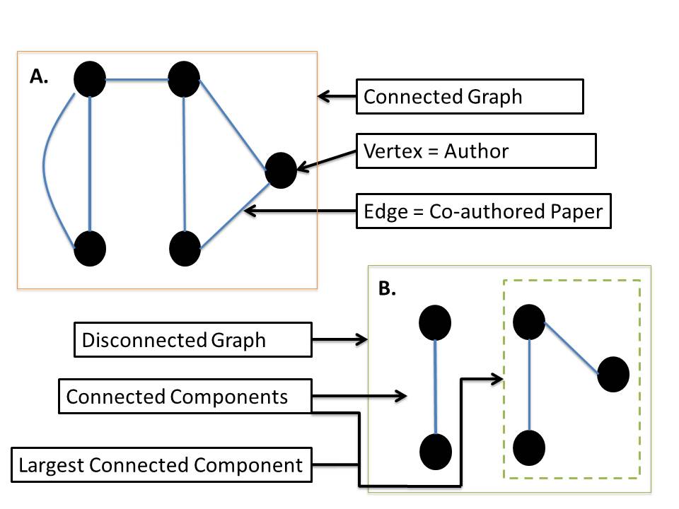
Networks are commonly represented by graphs. An example is seen in Figure 1 which shows a simplified co-authorship network. Here the individual vertices represent authors and the co-authored publications represent edges that connect the vertices. If two or more authors publish a paper together, then they are connected in the graph by the edge representing that paper. When a graph is formed, there may or may not be a path between all pairs of vertices. If there is a connecting path between all vertices in a graph, the graph is connected as seen in Figure 1A. Otherwise, the graph is disconnected as in Figure 1B. However, connected components (or simply components) exist in disconnected graphs. These are any group of vertices with a connection between all pairs of vertices. The graph in Figure 1B has two components, and the component in the dashed box is its Largest Connected Component (LCC). Co-authorship networks, when formed from enough authors and publications, will most often be disconnected and exhibit connected components of varying sizes.

Figure 1: Basics of graph representation and co-authorship network. This is a simple pictorial example of how a co-authorship network is represented by a graph. Vertices (dots) represent authors in the network while an edge (line) represents a paper that was co-authored by the authors it connects. Whereas each vertex is a unique author, an edge is not necessarily a unique paper. For example, the graph in A has 5 vertices and 6 edges. Therefore, the network represented by the graph definitely consists of 5 authors. However, based on this specific graph structure we cannot be certain if there are 4 or 6 papers. This is because the triangle formed on the right hand side can be formed by three papers, each written by two authors; or it could represent one paper written by all three authors where each edge represents the same paper. The example in A is a connected graph, while B is a disconnected graph. The network in B has 2 components where the component in the dashed box is its Largest Connected Component based on the fact it contains the most authors.

Figure 2: Graph representation of one of the co-authorship networks analyzed in this study. On the outer level, grouping first takes place as the network divides into many components. The network has a few large components consisting of many authors; the two largest are circled. Additionally, there are numerous small components, each formed by relatively few authors. In small components, relationships between authors are clear and can be easily identified with graph analysis tools. In large components, tightly bound groups known as communities form. This is the inner level of clustering. The communities are only loosely connected to other communities in the component. Thus, to identify which authors are collaborating closely, one must perform community detection on larger components.

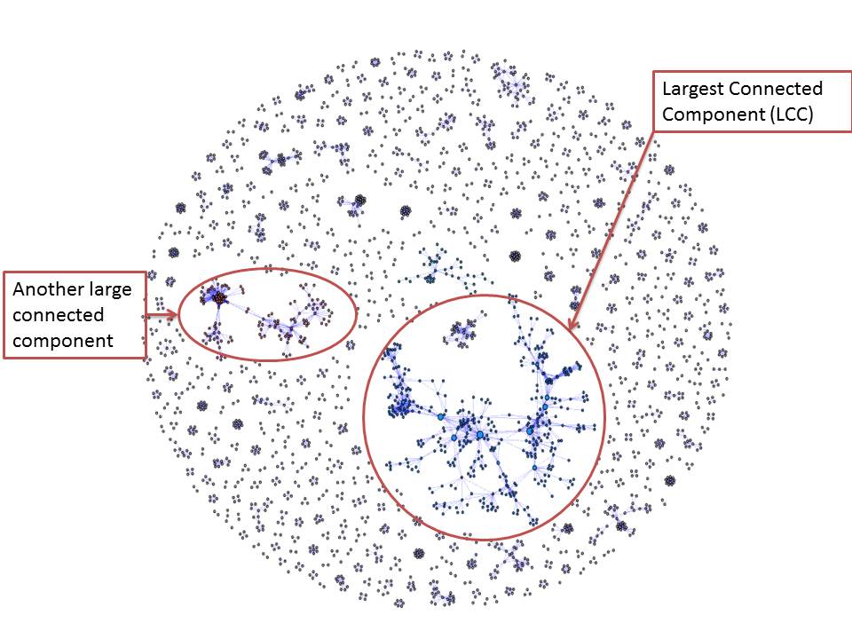
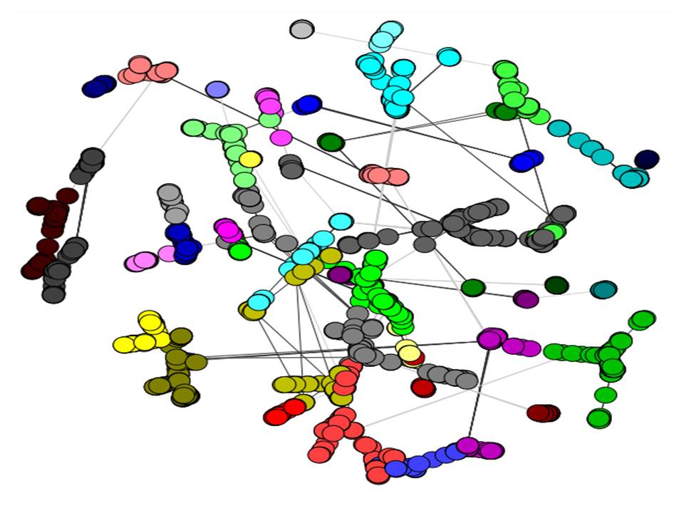
Co-authorship graphs are used to determine which scientists in the field are collaborating together. Then, based on available information about those scientists (such as papers they have written), one may infer what type of research is taking place in that group and where it is happening. In small components the relationships between authors are relatively easy to see and pick out using graph analysis tools. However, co-authorship networks, like those in Figure 2, can grow vast connected components with thousands of authors Newman2001_CoAuthorNet ; Barabasi2002590 . Though all the authors share common connections in a connected component of such magnitude, this does not imply that they are all actually working together. Instead, a few prominent researchers connect many different groups of researchers who in large part do not otherwise collaborate with each other Girvan11062002 ; palla2005uncovering ; Newman2001_CoAuthorNet . Co-authorship networks exhibit the following type of hierarchical clustering. The entire network is comprised of connected components of various sizes. This is the first level of groupings. Then, the larger connected components are composed of several tightly bound groups of authors loosely connected by a few co-authors common to more than one group. These tightly bound groups are the second level of clustering PhysRevE.69.066133 ; Newman2001_CoAuthorNet . Figure 2 illustrates a network with this hierarchical clustering structure and Figure 3 looks at the clustering present within a large component more closely. Gathering information about which authors are frequently collaborating within large components often requires detecting these smaller, more closely connected groups of authors, known as communities. There are many algorithms for community detection, each of which has its advantages and drawbacks. For example, oftentimes, some accuracy is sacrificed for savings in computation time Fortunato02012007 . Here we implement Newman and Girvan’s method of greedily optimizing modularity PhysRevE.69.026113 , known as fastgreedy. Figure 3 illustrates how communities were identified by fastgreedy within one of the large components used in this study. Each different color represents a community. Though it is difficult to see, many edges link vertices within communities. On the other hand, there are relatively few connections between communities. Thus, this component exhibits the hierarchical clustering structure described earlier.

Figure 3: Community Detection. Using Newman’s method of fastgreedy community detection, communities were identified within a large component similar to the LCC circled in Figure 2. This is the LCC of one of the networks analyzed in this study. Each different color represents a community. Notice the clustering present within the component. Though difficult to see, each community is tightly bound by a large number of co-authored papers within the group. However, the looser connections between the communities is quite clear as there are relatively few edges between groups.

Fastgreedy is well established and successful at picking out tightly bound groups from a whole. For example, it has been proven that fastgreedy can successfully infer the conference structure of NCAA Division I football by analyzing a graph in which vertices represent teams and edges represent games between teams PhysRevE.69.066133 . There are plenty of other case studies confirming the success of fastgreedy. Thus, we know that the results returned by this community detection generally provide an accurate representation of the scientific communities present in a graph. A question we pose is, do these communities reflect groups of researchers with an even narrower research focus than the component of which they are a part? In other words, does the hierarchical clustering present in the structure of the network imply a hierarchy on the specificity of research topic also? If this is true, consider, for example, forming a network of all authors who write about ‘animals’. One connected component would have authors who focus on ‘dogs’, while another group would be concerned with the study of ‘cats’. Within the ‘dogs’ group, we expect to see communities with authors more intently focused on subtopics such as ‘golden retrievers’ and ‘beagles’. Or, on the other hand, let’s assume that research topic specificity is not the case. Instead, only regional factors and institutional affiliations determine the hierarchy of the network. Then the United States would have its own component with authors writing papers about various topics in the ‘animals’ category. Within that component would be a community consisting of authors from the Cornell University College of Veterinary Medicine also writing about all types of animals. As a result, the communities would not represent groups of authors focused on a specific topic but rather groups of authors sharing a location and affiliation. Likely a combination of these factors, and others, determines the structure of the network and how communities are composed. However, in this study, we exclusively examine if the division of a component into communities implies that the individual communities are focused on more specific research goal topics than within the entire component.

In addition, this study also focuses on developing and validating an automatic way to determine the topics of a community. Our method utilizes bibliographic data from a database to form the network, community detection to pick out scientific communities within the network, followed by text analysis techniques to find the topics of those communities. By analyzing a community’s papers, these techniques extract important terms that are unique to the community. When examined together, the terms should provide a clear idea of the community’s topics. This approach will rely on a level of statistical confidence which requires that the communities evaluated be large enough to be statistically significant. Thus, we propose a minimum community size threshold- the community should have at least 8 papers or 15 authors- necessary to produce meaningful results from the procedure. If, through the use of this method, most communities are shown to exhibit increased concentration on certain terms, this is an indicator that the communities are indeed focused on specific research topics.

The remainder of the paper is divided into four sections. Section II describes the theory behind the text analysis techniques used to identify words that relate to the topic of a community. Section III describes the automatic method of using bibliographic data to form a network, followed by community detection, and the text analysis techniques we use to find terms that represent the topics of the communities. Section IV discusses the effectiveness of this method and suggests a minimum community size necessary for using the method. Section V summarizes the paper and discusses the implications this study has regarding the factors behind formation of scientific communities in co-authorship networks.

II Text Analysis Techniques

How do we determine if communities identified by a detection method represent groups of researchers publishing papers focused on a common topic? A qualitative way would be to isolate a community, gather its papers and then examine them for content. Of course, this is imprecise as differing opinions will lead to different conclusions about the cohesiveness of a community. Additionally, to do this manually for every community in a component would be laborious and time consuming. Here we present an automatic method to extract important terms from the publications of a community in order to identify the topic of the community.

Consider all the documents (this can either refer to the papers, or collections of words representing the content of the papers, such as the abstracts of papers) written inside a community created not by their authors, but by picking words one at a time at random from a set of possible words. This is a process known as sampling with replacement; it is like picking words from a "bag of words" where, after a word is picked and marked down, it is put back in the bag. For our experiment the universe of available words will be all the words present in any document in the component of which the community is a part. Continuing the example from Section I, let’s say the component focused on ‘dogs’ contained the words in the set $\Omega$={‘dog’, ‘golden retriever’, ‘puppy’, ‘beagle’}. Each word has a different probability of being chosen from the set which is estimated from examining how often the word appears in the community. Consider a community in which the probability of each word in the set $\Omega$ being picked was $P{}_{comm}=\left\{\frac{1}{3},\frac{1}{6},\frac{1}{3},\frac{1}{6}\right\}.$ Altogether the probabilities of every possible word in the sample space form a Probability Mass Function (PMF) from which to create, one word at a time, all the documents in a community. A document formed with $P{}_{comm}$ might look like this: [beagle dog beagle puppy golden retriever puppy puppy] where words don’t necessarily appear with frequency equal to their probabilities in $P{}_{comm}$ as the creation of the document is viewed as a random process. We can repeat this argument to conceive the formation of any document with an underlying PMF inferred not from the community to which it belongs, but instead from the entire component; call this PMF $P{}_{comp}$.

Assume now that the separation of the component into communities had no implications about focus on certain topics, i.e. the communities are properly separated, but their composition is determined by other factors besides striving towards a highly specific research goal. Then, a community would contain documents that have nothing more in common with each other besides the broader theme which defines the component. Thus, one would not expect any certain words to be significantly more probable within a community than throughout the entire component. We would expect to see the PMF of the community to look very similar to that of the component. In our example, if we had a community with $P{}_{comm}=\left\{\frac{21}{64},\frac{17}{64},\frac{11}{64},\frac{15}{64}\right\}$ and a component with $P{}_{comp}=\left\{\frac{1}{3},\frac{1}{4},\frac{1}{6},\frac{1}{4}\right\}$, all the words in $\Omega$ appear with nearly equal probability in the ‘dogs’ component and in the examined community. Thus, we would conclude that no terms are unique to the community. This implies the community is not focused on a topic more specific than ‘dogs’ and the division of the component into a community does not imply a narrowing of research focus.

On the other hand, consider picking out a community from the component in which scientists in the community pursued a mutual and specific research goal. For example, in a graph of authors who research and publish papers on dogs, we may have a group who concentrates on golden retrievers. We should expect to see words pertaining to that goal have a much higher probability of appearing in that community than in the component on the whole. In the example, we expect the probability of seeing ‘golden retriever’ in a document to be much higher in the community than in the component, while the probability of seeing ‘dog’ should be about the same in both. So now $P{}_{comm}$ and $P{}_{comp}$ might look like this: $P{}_{comm}=\left\{\frac{22}{64},\frac{1}{2},\frac{6}{64},\frac{4}{64}\right\},\>P{}_{comp}=\left\{\frac{1}{3},\frac{1}{4},\frac{1}{6},\frac{1}{4}\right\}$. In such communities, the words found to have a significantly higher probability of appearing in the community than in the component can be identified and then be further analyzed to determine the topic(s) of the community. Notice ‘golden retriever’ is the only word where $p{}_{comm}$ (lower case $p$ is used to denote the probability of one term appearing while capital $P$ denotes the entire PMF) is much greater than $p{}_{comp}$. Thus, in this very simple example, after examining the PMF’s of the community and the component, we would identify ‘golden retriever’ as a significant term and correctly conclude the community is concentrated on golden retrievers.

III Methodology

III.1 Forming a Co-authorship Network and Identifying Communities

III.1.1 Extracting Data From the Inspec Database to Form a Graph

We obtain the scientific publications necessary to form co-authorship networks using Thompson Reuter’s ISI Web of Knowledge v.5.5 index to access the Institute for Engineering and Technology’s Inspec publication database. The Inspec database contains an expansive collection of papers in the fields of mathematics, physics, and computer science. Once the Inspec database was selected through the Web of Knowledge search interface, the Boolean keyword or series of keywords best representing the sub-field under investigation were entered into the Inspec search field. The searches were carried out over the time span 1969-2012, the longest available in the database, although most searches returned a group of publications spanning a shorter period. A keyword search usually returned anywhere from $10^{1}$ to $10^{5}$ papers. Using a custom Python script, the data was pre-processed by sub-fields to extract a list of authors. The authors’ last names and initials were stored, while repetitions were removed. Information, such as papers written and affiliation, was stored for each author. The same was done for each paper returned by a search; information such as the paper’s authors and the string of key terms used to identify the topic of a paper were extracted and stored.

III.1.2 Creating a Graph and Identifying Communities

The data from the publications was used to create a co-authorship network. As mentioned before, to begin forming a graph, each author is considered to be a vertex and an edge between two vertices is formed for every paper that the two researchers co-authored together. Again, there is most often not a path connecting all vertices in the graph, and we see several connected components. Though a graph may have a few large connected components, per graph we will only focus on the LCC. Graphs will exhibit hierarchical clustering as the larger connected components contain several groups of strongly interconnected vertices within them. To pick out these communities in the LCC, the fastgreedy community detection method was used.

III.2 Extracting Key Terms to Represent Documents, Forming PMF’s with Estimates of $p$ for Each Key Term

III.2.1 Extracting Key Terms to Represent the Content of the Papers

Each paper provides key terms under a ‘Topics’ field that is useful for searching the paper in a database. These terms provide a very succinct representation of the content of a publication and will be our device for inferring topic focus, or lack thereof, within communities. They will serve as the ’words’ discussed in Section II, while a paper’s collection of key terms will form the ‘documents’. A paper will have anywhere from 5 to 70 key terms with an average paper containing 15 to 25 terms. This is a valid substitute for analyzing the entire text of a paper because the key terms summarize the most useful information (from the viewpoint of this study) that could be drawn from a paper by identifying the topics of a paper. Additionally, it is possible to circumvent analyzing the occurrences of common words that would appear with about equal frequency in almost any paper, such as ‘the’ and ‘a’. Furthermore, by avoiding analyzing all the text in every paper, computation time is significantly reduced by only performing the text analysis techniques on the papers’ key terms.

A custom Python script was written to identify each key term present in the ‘Topics’ fields of a paper. We used this to identify all unique key terms in the LCC of a graph. Several key terms had the same meaning, but were identified as distinct terms due to spelling or phrasing differences. For example, ‘dog’ and ‘dogs’ would be distinct terms. However, since their meaning is the same, and this method is concerned with identifying topics, it would make sense if they were viewed as the same term. For this reason, groups of key terms with slight spelling or phrasing differences were identified and one of the key terms was used to represent the entire group. Whenever any term in the group appeared in a paper’s ‘Topics’ field it was replaced by the group’s representative key term. Once these meaningless spelling or phrasing differences were accounted for, we repeated the process of finding all unique key terms in the LCC to form our set of words, $\Omega$.

III.2.2 Estimating $p$, the Probability of a Word Being Chosen to Form a Document

Taking the view discussed in Section II in our analysis, that documents are formed by sampling words from a set using the PMF of the community to which it belongs, we first excluded papers that overlap into two or more communities to avoid situations where a paper is formed by more than one PMF. Fortunately this is a small percentage of the total papers in a component as communities will be linked by a few papers, but a large majority of the papers are contained entirely within the individual communities.

Then, for each key term in $\Omega$, a count was kept of the number of papers in which that term appeared within each community and also the total number that it appeared in the entire LCC. Let this count equal $k$; $k_{comm}$ for the count within a community, $k{}_{LCC}$ for the count within the LCC. Additionally the total count of all key terms was recorded for both the communities and the LCC. This is not counting unique key terms, but rather it is a sum of the number of key terms in all the papers in a community or the LCC. Let this total count equal $n$; again $n{}_{comm}$ for within a community, and $n{}_{LCC}$ for the LCC. Another way to think of $n$ is that it is the sum of all the counts within the group of interest for all terms belonging to $\Omega,$ so $n_{comm}=\sum_{\left\{terms\in\Omega\right\}}k_{comm}$ and $n{}_{LCC}=\sum_{\left\{terms\in\Omega\right\}}k_{LCC}$. In each case, $k$ can be thought of as an observation of $K$, a binomially distributed random variable with parameters $n$ and $p$. Here, $p$ is what we are seeking to form a PMF for the community/LCC. However $p$ is unknown to us as we only observe $k$ and $n$. Thus we needed an estimate, $\hat{p}$, of $p$ based on $n$ and our sole observation of $K$. A simple estimate of $p$ would be the point estimate $\hat{p}=\frac{k}{n}$; this is how the normal approximation to the binomial estimates $p$. However, when $p\times n\leq 5$, $\hat{p}=\frac{k}{n}$ is proven to be an unreliable estimate of $p$ brown2001 . Since key terms typically exhibited very low counts, $k$, compared to total words, $n$, we assume it is likely that the true probability, $p$, was very small also. Then, for many key terms $p\times n\leq 5$, and using $\hat{p}=\frac{k}{n}$ would not be a reliable estimate. Thus, to test the appropriateness of other methods for estimating $p$ over ranges of possible $k$ and $n$ seen in this study, the following experiment was performed.

Given a term has true probability $p$ of being picked from a set, consider a trial in which choosing that term is a success and picking any other term is a failure. This describes a Bernoulli trial with probability $p$ of success and can be represented by flipping a biased coin with the probability of heads appearing equal to $p$. Repeating this trial $n$ times will result in a binomial distribution for the random variable $K$ representing the number of heads that appear in $n$ flips of the coin where the probability of observing $k$ heads in the $n$ flips is: $P(K=k)={n\choose k}(p)^{k}(1-p)^{n-k}$ for $k=0,1,2,...,n$. Using a $p$ commonly seen in key terms within a community, we perform $n$ trials, observe $k$ heads, and then compute $\hat{p}$ with it’s (1-$\alpha$) confidence interval (CI) utilizing the following approximations of the binomial parameter $p$ agresti1998approximate :

$$Wald^{\prime}s/Normal:\>\hat{p}=\frac{k}{n}\>\>\>CI:\>\hat{p}\pm z\sqrt{\frac{\hat{p}(1-\hat{p})}{n}},$$

$$Agresti-Coull:\>\hat{p}=\frac{k+\frac{1}{2}z^{2}}{n+z^{2}}\>\>\>CI:\>\hat{p}\pm z\sqrt{\frac{\hat{p}(1-\hat{p})}{n+z^{2}}},$$

$$Continuity\>Corrected\>Wilson\>Score\>Interval:\>\hat{p}=\frac{k+\frac{1}{2}z^{2}}{n+z^{2}}\>\>\>CI:\>(a,b),$$

$$where:\>a=max\left\{0,\frac{2k+z^{2}-\left(1+z\sqrt{z^{2}-\frac{1}{n}+4k(1-\frac{k}{n})+(4\frac{k}{n}-2)}\right)}{2\left(n+z^{2}\right)}\right\},$$

$$and\>b=min\left\{1,\frac{2k+z^{2}+\left(1+z\sqrt{z^{2}-\frac{1}{n}+4k(1-\frac{k}{n})-(4\frac{k}{n}-2)}\right)}{2(n+z^{2})}\right\},$$

where $z=z{}_{\alpha/2}$, the value at which the standard normal cumulative density function is equal to $1-\frac{\alpha}{2}$, and $\alpha=$one minus the desired confidence level as a fraction. Here, $z=1.96$ at a 95%, (1-.05), confidence level, the confidence level used throughout the study. The interpretation of a confidence interval is fairly simple. If given a CI, $\left(a,b\right)$, for $p$ at 95% confidence where $a$ and $b$ are determined by the observation of $K$, ideally 95% of the observations of $K$ will give $a$ and $b$ such that $\left(a,b\right)$contains the true $p$ (for a general reference on approximations to binomial proportions and confidence intervals see Ref devore2012probability ). This is not always the case and actual coverage probabilities, the probability that a CI formed from a random observation of $K$ will contain $p$, often differs from the desired confidence level, especially at small $n$ and $p$. The amount this coverage probability varies from the desired confidence level also depends on the confidence interval that is used brown2001 .

Notice in the above equations that both the Wilson and Agresti-Coull confidence interval have the the same $\hat{p}$, however the lengths and endpoints of the confidence intervals differ. We perform the test on a range of $n$ values reflecting typical key term totals seen in the communities recording $\hat{p}$ for each method and value of $n$. We repeat the experiment 10,000 times. For each method, the sample standard deviation of the $\hat{p}$ values as a percentage of $p$ was recorded for every value of $n$ tested. This is an indicator of the reliability in the estimates of $p$. As $\hat{p}$ is the same in both the Agresti-Coull and Wilson’s Interval, we expect this experiment to give nearly identical results for the two, however the difference in the widths of their confidence intervals will prove to be more important later in the study. The same procedure is repeated for values of $n$ and $p$ reflecting typical values seen in the entire LCC of a graph.

Using the estimate we deem best suited for our study, for every key term we were able to obtain an estimate of $\hat{p}_{comm}$ for every community and $\hat{p}{}_{LCC}$ along with 95% confidence intervals for each $\hat{p}$.

III.3 Determining a Community’s Significant Key Terms

As stated before, for each $\hat{p}$ there exists an error associated with the estimate related to the width of the (1-$\alpha$) confidence interval, $W$. Analogous to how the standard deviation, $\hat{\sigma}_{Wald}$, in the estimator $\hat{p}_{Wald}$, is $\hat{\sigma}_{Wald}=\nicefrac{{1}}{{2}}(\frac{W_{Wald}}{z_{\alpha/2}})$, we will consider the standard error, $\delta$, in our estimates $\hat{p}$ to be $\delta=\nicefrac{{1}}{{2}}(\frac{W}{z_{\alpha/2}})$. Thus, each key term has a $\hat{p}{}_{LCC}$ with error $\delta{}_{LCC}$ and in each community a $\hat{p}_{comm}$ with error $\delta_{comm}$. To determine a community’s significant key terms, find terms such that:

$$\hat{p}_{comm}-\hat{p}_{LCC}>\beta\left(\sqrt{\delta{}_{comm}^{2}+\delta_{LCC}^{2}}\right)$$

where $\sqrt{\delta{}_{comm}^{2}+\delta_{LCC}^{2}}$ attempts to capture the uncertainty present in the difference $\hat{p}_{comm}-\hat{p}{}_{LCC}$ and $\beta$ is a constant that controls how many standard deviations $\hat{p}_{comm}$ has to be above $\hat{p}{}_{LCC}$ for a term to be considered significant. Choosing $\beta$ too small will result in too many key terms being deemed significant and one still would not have a clear idea of the topic of the community. Additionally, with small $\beta$, it is much more likely for some of the returned key terms to have true values of $p{}_{comm}$ not greater than $p{}_{LCC}$, but due to estimation error, will have $\hat{p}_{comm}-\hat{p}_{LCC}$ above the minimum threshold. Choosing $\beta$ too large will likely result in the wrongful identification of all key terms as insignificant. We chose $\beta=2$ for this study such that a select few key terms were returned and, for these key terms, $p{}_{comm}$ is almost certainly higher than $p{}_{LCC}$ due to focus on that term in the community and not because of errors in our estimates $\hat{p}_{comm}$ and $\hat{p}_{LCC}$. The more significant key terms identified from this analysis, the greater evidence of topic focus in that community.

III.4 Determining a Minimum Threshold for Community Size

Due to the increasing error in the estimation of $p$ as $n$ decreases, performing this analysis becomes less likely to return significant key terms as the number of total terms in the community decreases. Therefore, it is expected that this analysis becomes far less effective and useful below a certain community size.

Community size can be defined in several ways. From a more general co-authorship network analysis viewpoint, it can be defined as the number of authors or the number of papers in a community. More applicable to this study is community size in terms of total key terms contained in all of a community’s papers. By plotting the number of significant key terms versus community size for each of these community size metrics, we attempted to identify a minimum threshold community size according to each measurement for use of this analysis. This is intended to serve as a guideline for which communities it would be prudent to use this method to identify their topic.

IV Results/Discussion

IV.1 Choosing an Estimator for $p$, Finding a Range of $n$ where the Estimate is Reliable

IV.1.1 Choosing the Estimator

Figure 4: Sample standard deviation of 10,000 estimates of $p$ as a percentage of $p$ versus number of tosses of a biased coin with probability of heads appearing $p=0.01$. This is an indicator of reliability in the estimator $\hat{p}$ for different values of $n$, the number of Bernoulli trials performed, at true $p=0.01$, a value expected for a borderline significant key term. The range of $n$ is chosen to represent typical amounts of total terms present in smaller communities. Three methods are used to calculate $\hat{p}$: Wilson’s with Continuity Correction (dashed), Agresti and Coull’s (dotted), and Wald’s (solid line). The graph shows the Wilson and Agresti-Coull estimators have less variability at small $p$ ($p=0.01)$ and small $n$, while all three have very similar standard deviation at > 200 trials. This suggests that either Wilson’s or Agresti and Coull’s estimate and confidence interval should be used throughout the study. Additionally, it points out that any estimate of $p$ below 150 terms has great uncertainty as the standard error in the estimator is near or above 100% of the true $p$.

Figure 5: Sample standard deviation of 10,000 estimates of $p$ as a percentage of true $p$ versus number of tosses of a biased coin with $p=0.001$. This determines the variability in the estimator $\hat{p}$ for different values of $n$, the number of Bernoulli trials performed, at true $p=0.001$, a value expected for terms across the entire LCC. The range of $n$ is chosen to represent typical amounts of total terms present in the LCC of a graph. Again, three methods are used to calculate $\hat{p}$: Wilson’s with Continuity Correction (dashed), Agresti and Coull’s (dotted), and Wald’s (solid line). All estimates have nearly the same standard deviations here, so any decisions for which estimate to use for the procedure should be based off of considerations for estimating $p{}_{comm}$, not $p{}_{LCC}$. Additionally, the errors $\delta{}_{LCC}$’s are much smaller than $\delta{}_{comm}$’s. For example, 25% of 0.001 is much less than 100% of 0.01. Thus when finding the error in the difference of the estimates $\hat{p}_{comm}-\hat{p}{}_{LCC}$, most will be determined by the error present in the estimator $\hat{p}_{comm}$.

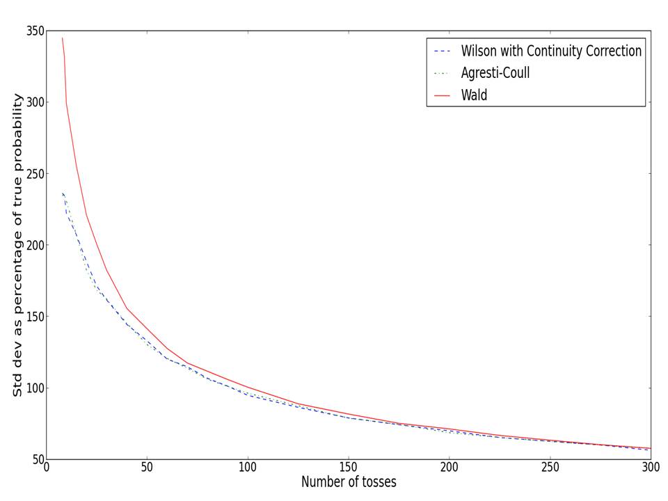
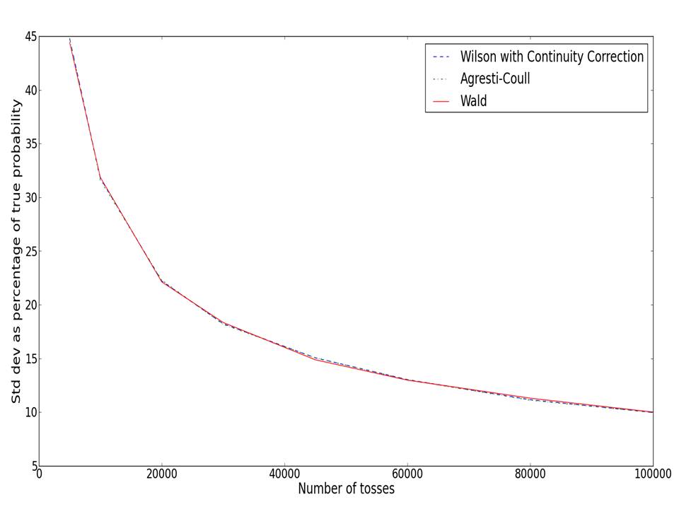
Figure 4 shows that estimating the true probability, $p$, of success in a Bernoulli trial based on one observation of the count, $k$, of successes in $n$ trials becomes less and less reliable as $n$ decreases and the standard deviation of $\hat{p}$ increases greatly. This is especially true for small $p$, which we will be dealing with in a large majority of key terms. As mentioned before and confirmed in Figure 4, Wald’s estimate of $p$ performs the worst for small $p$ and $n$ as there is great uncertainty in the measurement. Wilson’s and Agresti-Coull’s perform better below $n=200$, a common number of total terms for small communities, at $p=0.01$, a typical value for a key term’s $p{}_{comm}$, suggesting one of these two should be used as the primary estimator for the procedure described in Section III.C. Wilson’s and Agresti and Coull’s estimators $\hat{p}$ are calculated the same way, so no difference is seen in the variability of the estimator here. However, as stated before, the widths, endpoints, and effectiveness of the 95% confidence intervals are the determining factor for which estimate and confidence interval to choose for determining significant key terms. According to the study of different binomial confidence intervals done by Brown, Cai, and DasGupta, the Continuity Corrected Wilson confidence interval has a shorter expected confidence interval width than Agresti and Coull’s while maintaining an actual coverage probability closer to the desired 95% than Agresti and Coull’s especially in for small $p$ and $n$ brown2001 . Therefore, based on the superior performance of the Continuity Corrected Wilson confidence interval in estimating $p{}_{comm}$, if it also performs at least as well as the other two estimators in estimating $p{}_{LCC}$, we should find it proper to use this estimator and confidence interval for the remainder of the study. As a test of each estimate’s performance in estimating $p{}_{LCC}$, the three different estimates are evaluated again, but now at $p=0.001$, a common $p{}_{LCC}$, and $n$ values representative of typical values seen in a LCC. Figure 5 shows that all three estimators are equally variable for such values of $n$ and $p$. It follows that any decisions for choosing an estimator for the procedure should be based off of how the estimator performs estimating $p{}_{comm}$, not $p{}_{LCC}$. Thus, this result confirms our choice to use Wilson’s confidence interval with Continuity Correction as the estimator to implement the procedure described in Section III.C.

IV.1.2 Range of $n$ where $\hat{p}$ is Reliable

Another noteworthy feature of Figure 4 is that, even when using Wilson’s estimate, the standard error in the estimator will be great compared to the true value of $p$ - around or above 100% of $p$ - when $n$ is less than 150. This suggests that our method of comparing community and component PMF’s to determine significant key terms in a community, which relies on a moderately accurate estimate of $p_{comm}$, may not be a reliable or effective procedure for determining the topic of communities with less than around 150 total terms. Further analysis of 150 terms as a minimum community size threshold takes place in Section IV.B.3.

Figure 5 shows us that the errors in $\hat{p}_{LCC}$ will be much less than the errors in $\hat{p}{}_{comm}$, both as a percentage of true $p{}_{LCC}$ and in total error. This is because 10% to 45% of 0.001 is much less than 50% to 200% of 0.01. Though the error in $\hat{p}_{LCC}$ is present and affects the error in the difference $\hat{p}_{comm}-\hat{p}{}_{LCC}$, it is almost negligible compared to the error in $\hat{p}{}_{LCC}$. However, to err on the side of caution, we still consider the standard error in the difference $\hat{p}_{comm}-\hat{p}{}_{LCC}$ to be $\sqrt{\delta{}_{comm}^{2}+\delta_{LCC}^{2}}$, the sum of the errors in quadrature.

IV.2 Finding Significant Key Terms that Determine the Topic of a Community

IV.2.1 A Look at How Significant Key Terms Represent the Topic of a Community

Utilizing the Continuity Corrected Wilson confidence interval at 95% and the $\hat{p}$ that accompanies it, the procedure for finding significant key terms in Section III.C was performed on networks of various sizes. The following is an example of some results achieved from using this method. In a network formed by searching the term ‘neuromorphic computing’ in Thompson Reuter’s ISI Web of Knowledge v.5.5 index according to Section III.A, 918 papers were returned to form the network which also contained 1414 unique authors. This is one of the smaller networks analyzed in this study. The LCC was formed by 270 papers and 370 unique authors. One of the communities within the LCC contained about 25 papers. Representative titles include: ‘Analog VLSI models of range-tuned neurons in the bat echolocation system’, ‘Analog VLSI circuits for attention-based, visual tracking’, and ‘A Neuromorphic VLSI Head Direction Cell System Online Correction of Orientation Estimates Using Spatial Memory in a Neuromorphic Head Direction System’. Several significant key terms were returned for this community. Among them included: ‘VLSI’, ‘visual information’, ‘motion estimation’, ‘mechanoreception’, ‘bioacoustics’, ‘biomimetics’. Although the sample size is small, the qualitative match between the significant key terms and the titles seems to accurately reflect the themes of the papers. Therefore we argue it is acceptable to use these terms to represent the topic of the community.

IV.2.2 Quantitative Measures for the Amount of Focus on a Topic

As a quantitative measure of community focus, we could look at the number of significant key terms in a community. If a community is focused on a topic, we expect to see a lot of key terms related to that topic repeated in several papers, causing a high $\hat{p}_{comm}$ for those terms and consequently being marked significant. Conversely, if a community is unfocused, there will be plenty of key terms, but few will be repeated in more than one paper. In this case, for most terms $\hat{p}_{comm}$ will not differ much from $\hat{p}{}_{LCC}$. When a community does have only a few significant terms it could be the result of the following two characteristics of communities: 1) either there is actually not much focus on any topic in the community, or 2) the community was not large enough to obtain enough total terms for a reliable estimate of $p{}_{comm}.$ If 1) is true, that will result in small differences of $\hat{p}{}_{comm}-\hat{p}{}_{LCC}$ for nearly all terms, such that $\hat{p}{}_{comm}-\hat{p}{}_{LCC}$ does not exceed $2\sqrt{\delta{}_{comm}^{2}+\delta_{LCC}^{2}}$, our minimum threshold for marking a key term significant. If 2) is true, it causes a large error in $\hat{p}_{comm}$ as seen in Figure 4, driving the error in $\hat{p}_{comm}-\hat{p}{}_{LCC}$ up enough that even terms with moderately sizable differences in the estimates of $p{}_{comm}$ and $p{}_{LCC}$, $\hat{p}_{comm}-\hat{p}_{LCC}$ will not be greater than $2\left(\sqrt{\delta{}_{comm}^{2}+\delta_{LCC}^{2}}\right).$ In either case, we are not able to determine the community’s topic, if there is any clear topic, from our analysis.

The arguments presented in the previous paragraph seem to suggest using the percentage of unique key terms in a community that are significant as a measure of the amount of focus in a community. However, we caution against using this measure when comparing communities with a large difference in size. To see why, first consider a community with only 50 unique terms. Having just 3 of them be marked significant results in a 6% percent rate. On the other hand, in a large community, with a much larger sample size, say 1000 unique terms, having 50 significant key terms results in a 5% rate. It’s not clear which is really more focused: a community with a small sample size and only a few significant key terms, but a higher significance rate; or a large community with many more total terms and significant terms, but a lower success rate. Therefore, we recommend only using this measure to compare communities with similar size.

IV.2.3 Determining a Minimum Community Size Threshold for Using this Analysis

Throughout the paper it has been suggested that this analysis may not perform well in smaller communities where the total number of terms is relatively low. In Section IV.A it was suggested that the analysis would not be effective in communities with less than 150 terms. In an attempt to show that 150 is a reasonable lower limit on the number of total terms needed to use this analysis on a community, the number of significant key terms per community versus community size in total terms was plotted in Figure 6 with data from eight different networks.

Figure 6: (Color Version Online) A. Number of significant terms per community versus community size measured in total terms per community. Communities from 8 different networks of various sizes ranging between 800 to 15000 publications are plotted here. It is clear that as the number of total terms in the community increases, so does the number of significant key terms. The fact that most communities contain many of these community-specific significant key terms is an indicator that, in general, scientific communities in co-authorship networks are focused on researching a specific subtopic of their field. B. Similar plot to A, focused on the densely populated region near the origin. The dot sizes indicate how many communities share the same (x,y) data point. The larger dots indicate there are 2 communities at that point while the smaller dots indicate there is 1 community at that point. A noticeable change in the graph occurs at 150 terms. Above this point, significant key terms are almost always present in communities, and the number of these significant key terms is occasionally high enough to make some conclusions about the topic of the community. Below this point, often no significant key terms are identified in the communities, and most of the time less than 5 terms are marked significant. Our method to identify a community’s topic is therefore not effective in communities with less than 150 total terms.

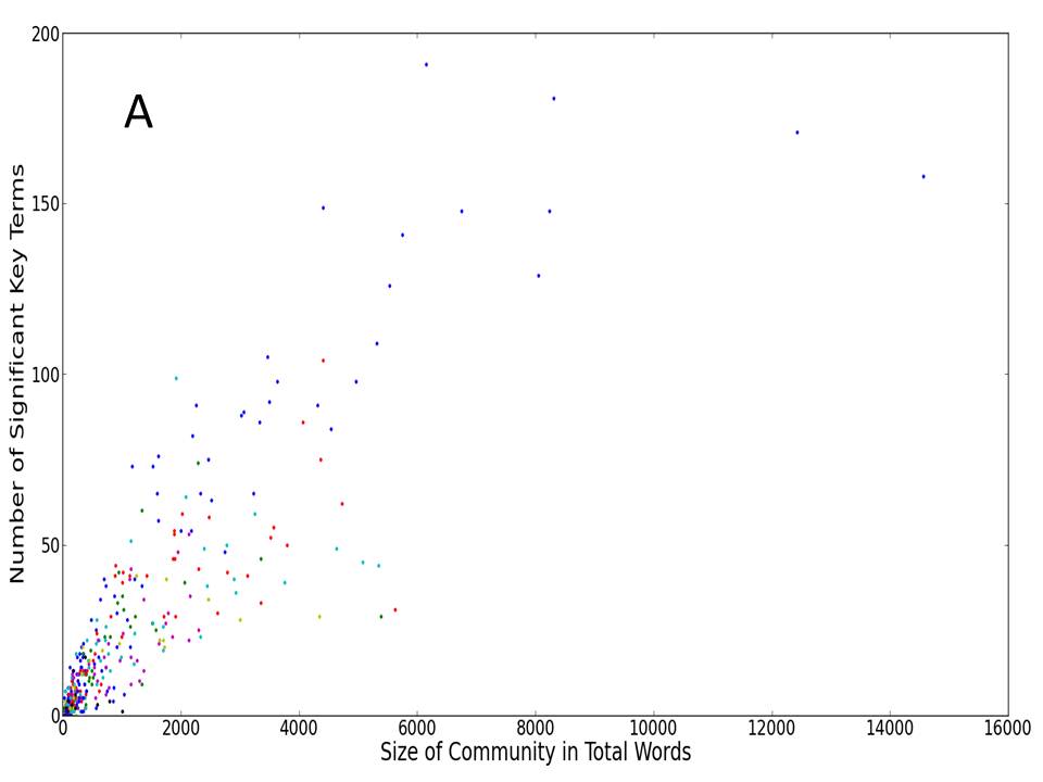
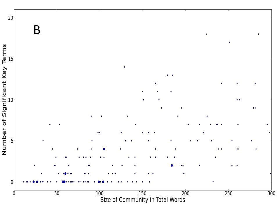
In Figure 6A, we see more significant key terms are returned as community size increases. One reason larger communities have more significant terms is that estimates of $p{}_{comm}$ become less variable in communities with large $n{}_{comm}$. This causes the error $\delta{}_{comm}$ to be smaller, and differences in $\hat{p}{}_{comm}-\hat{p}{}_{LCC}$ are more likely to be above $2\sqrt{\delta{}_{comm}^{2}+\delta_{LCC}^{2}}$. Thus, our procedure is more effective in picking out significant terms because we are getting more precise estimates of $p_{comm}$. A more obvious reason for this is that there simply aren’t as many unique terms in small communities to choose from. Recall that the number of total terms is not the same as the number of unique terms, but they are closely related. Community size in total terms is equal to $n_{comm}$, which is $\sum_{\left\{terms\in\Omega\right\}}k_{comm}$, the sum of all the counts for each term in $\Omega$ within the community, whereas the number of unique terms in a community is the number of the terms belonging to $\Omega$ such that $k{}_{comm}\neq 0$. Communities with larger $n{}_{comm}$’s tend to have more unique terms which leads to more possibilities for significant key terms. However, this alone is not a guarantee there will be any significant key terms. As discussed earlier, a community, large or small, without a clear topic will have little or no significant key terms. The fact that communities with enough terms consistently return large numbers of significant terms indicates many communities are focused on specific topics. Next, we look at how the analysis performs in communities without enough terms, and ascertain the minimum number of terms necessary for the analysis to be effective.

As seen in Figure 4, the variability of $\hat{p}_{comm}$ starts to increase significantly below $n=150$. Thus, in Figure 6B we focus on the range of sizes near 150 terms to determine if this is the right minimum threshold to use. At less than 150 terms, the procedure for identifying significant key terms will return no significant terms about half the time and less than 5 significant terms most of the time. This is often not a large enough sample size of significant key terms to deduce the topic of a community. So, whether the low significant key term count is due to the lack of enough terms, or the increasing error in $\hat{p}_{comm}$, or both, the procedure is most often ineffective in communities with less than 150 total terms. This agrees with the inference made about the effectiveness of the procedure in communities with less than 150 terms made in Section IV.A. In communities with size slightly above the threshold at about 150-300 terms, rarely does this method return no significant key terms, and sometimes upwards of 10-15 terms are returned. Thus, the procedure is worth trying in this range of $n$. Finally, as seen in Figure 6A, communities with greater than 300 terms almost always return many significant key terms.

Though community size in total terms is very applicable to this study, community size is rarely measured by the amount of total key terms present in the ‘Topics’ fields of the papers present in that community, but rather, often measured by number of authors or papers. However, this analysis allowed us to form a connection between the community size and the number of significant key terms in a community. And, using this relationship, we can extend the conclusions to find thresholds for the more common measures of author number and paper count.

The relationship between the size of the community in papers and the size in total terms is fairly straightforward. It is positively correlated, as the number of papers increases, the number of key terms generally increases also. Although, this is not always the case as there is no set number of key terms per paper. So, for example, it is possible for a community containing 20 papers to have more key terms than a community with 25 papers if some of the authors in the 20-paper community prefer to tag papers with many key terms. There is a very strong correlation, 0.992, between papers and terms though, so we expect plotting the number of significant key terms versus community size in papers to reveal similar patterns to Figure 6. Figure 7 confirms this is indeed the case.

Figure 7: (Color Version Online) A. Number of significant terms per community versus community size measured in number of papers per community. Communities from 8 different networks of various sizes ranging between 800 to 15000 publications are plotted here. Each different color represents communities from a different network. There is a nearly identical relationship between number of significant key terms in a community and community size in papers as seen in Figure 6 which plotted significant key terms versus size in total terms. This is because of the strong correlation between the number of papers in a community and the number of total terms present. B. Similar plot to A, focused on the densely populated region near the origin. The dot sizes indicate how many communities share the same (x,y) data point. The largest dot size represents 13 communities while the smallest dots indicate 1 community at that point. Using the same arguments to pick a minimum community size threshold for recommended use of this procedure that were used to determine a threshold for size measured in total terms, we suggest using this method in communities with more than 8 papers..

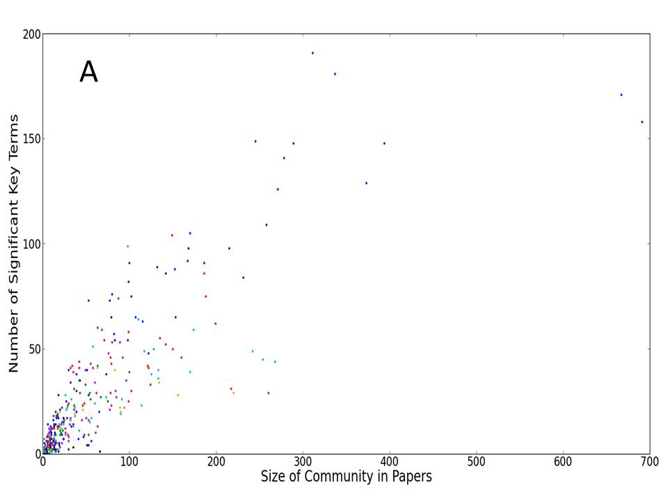
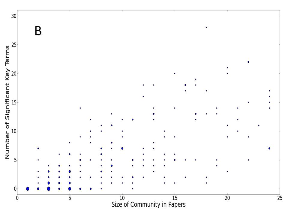
Nearly all the same arguments used to choose a minimum size threshold for number of terms apply here as well. The only difference is that having less papers only strongly implies there will be less terms, but it isn’t a certainty. After that, the rest of the logic follows as before. 8 papers appears to be the right threshold here. Additional analysis of our data shows that a paper contains, on average, 21 key terms. Since the correlation between community size in papers and terms is very strong this indicates that a communities with 7 papers would tend to have about 142 terms (below the term threshold) while communities with 8 papers should have near 163 terms (above the term threshold). This additional data supports the choice of 8 as a threshold for community size in papers.

Finally, the relationship between the number of authors in a community and the number of terms in a community is only slightly more complicated. Firstly, the size of a community in authors is strongly positively correlated with the size in papers. Although, a paper can have anywhere from 1 to over 100 authors Newman2001_CoAuthorNet , so, much like the relationship between papers and terms, a community can have less authors than another but more papers. Then, as described earlier, the community size measured in papers is strongly correlated with the size in total terms. As a result of this, the correlation between the number of authors in a community and the number of terms- 0.917- is less than the correlation between the number of papers in a community and the number of terms- 0.992. This being said, we still expect many of the same patterns to appear in the plot of the number of significant key terms in a community versus the community size measured in authors as in the previous two cases.

Figure 8: A. (Color Version Online) Number of significant terms per community versus community size measured in number of authors per community. Communities from 8 different networks of various sizes ranging between 800 to 15000 publications are plotted here. Each different color represents communities from a different network. There is a very similar relationship between number of significant key terms in a community and community size in authors as seen in Figure 6 which plotted significant key terms versus size in total terms. However, there is less correlation between number of significant key terms and size in authors than between number of significant key terms and size in terms. B. Similar plot to A, focused on the densely populated region near the origin. The dot sizes indicate how many communities share the same (x,y) data point. The largest dot size represent 7 communities at that point while the smallest dots indicate there is 1 community at that point. Using the same arguments to pick a minimum community size threshold for recommended use of this procedure that were used to determine a threshold for size measured in total terms, we suggest using this method in communities with more than 15 authors.

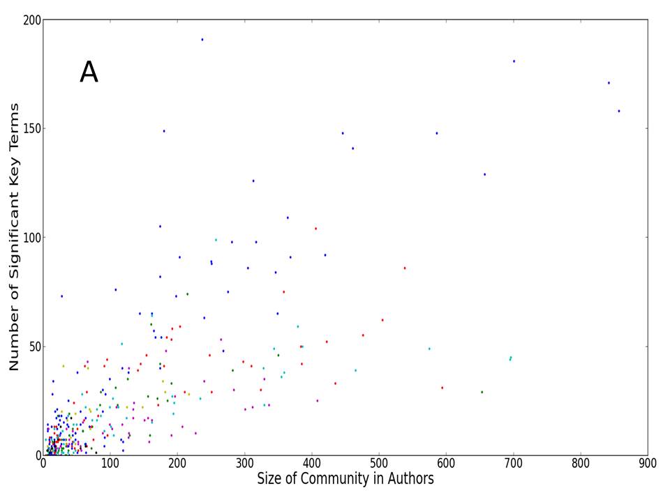
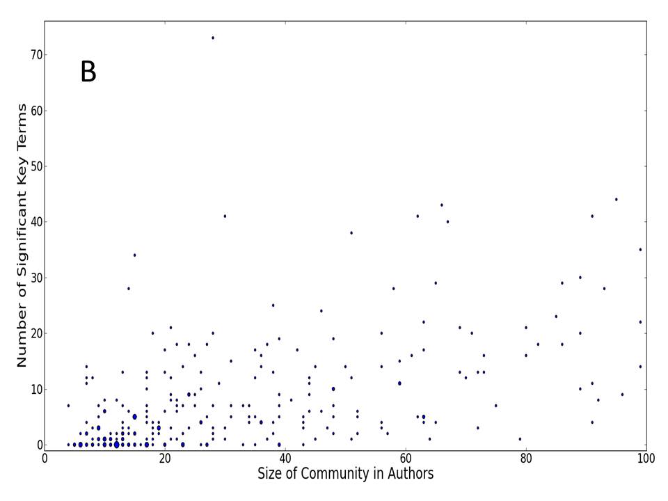
Figure 8 shows that many of the same patterns exist, however the correlation between significant key terms in a community and community size in authors isn’t as strong as for the previous two measures of community size. This is likely due to slightly decreased correlation between the number of authors and the number of terms in a community because of the more complex relationship between the two. Using the same criteria for picking a threshold as before, we choose 15 authors as the minimum threshold for this procedure to be somewhat effective (with effectiveness increasing with size). Additional analysis of our data shows that, on average, there are 10.5 key terms per author in a community. Since the correlation between community size in papers and authors is fairly strong at 0.917 this indicates that a community with 15 authors would tend to have slightly above 150 terms while communities with 14 authors are expected to contain slightly below 150 terms. This additional data supports the choice of 15 as a threshold for community size in authors. Though if one was choosing between the two more common size measures- authors and papers- we would suggest using community size in number of papers and the threshold that corresponds to that size metric. This is because there is greater clarity in how the number of papers affects the number of total terms. Furthermore, by comparing Figures 7 and 8, one can see there are more communities with author size above the 15 author threshold where the analysis fails to produce significant key terms than with paper size above its 8 paper threshold. Because the relationship between the number of authors and total terms is more complicated (and less correlated), it is difficult to tell if the absence of significant terms in these communities is a result of lack of focus on a topic or because the community is below the 150 term threshold (the strongest threshold for this procedure). Conversely, if a community is above the paper threshold, it is most likely above the 150 term threshold too. In summary, the 8 paper threshold, while not as significant as the 150 term threshold, is more accurate than the 15 author threshold.

V Conclusion

We have found an automatic method of using bibliographic data to determine the research focus of communities present in co-authorship networks that is most often successful in producing a representation of a community’s topic. By detecting key terms with a statistically significant greater probability of appearing in a community than in the community’s component, we were able to find many significant key terms per community. Then, through an inspection of a community’s significant key terms, one can deduce the community’s topic.

Small communities are the exception where this method is not effective. For a variety of reasons, few, or even no significant key terms are returned. This is not necessarily an indicator that the community lacks focus on a topic, but simply that there limitations in this procedure which prevent us from being able to determine the topic of small communities. Thus, a recommended community size threshold is proposed for three different community size measures, above which one will start to see some useful results from this method. For community size measured in total terms: 150 terms; for community size measured in papers: 8 papers; for community size measured in authors: 15 authors (though we recommend using either of the first two community size thresholds for analysis with this method). When these size requirements are met and the method returns enough significant key terms, we have seen qualitatively that examining those terms does, in fact, give an accurate representation of the topic of the community.

Now, recall the question posed in the introduction: does the hierarchical clustering present in the structure of the network imply a hierarchy on the specificity of research topic also? The results produced from the method to find significant key terms provide evidence that this is the case. The method used was designed to pick out community specific key terms: terms that appeared with great frequency in the community, but not throughout the component. Most communities that were large enough for this procedure to produce interpretable results contained several of these community specific key terms. Since these terms represent the topic of the community, it follows that the community has a specific and unique topic. Thus, the division of the component into communities is significant in the sense that it marks the division of a larger group of scientists researching a more general topic common to the entire component into small groups of researchers focused on researching a specific subtopic of the field.

References

- [1] Nasrullah Memon, HenrikLegind Larsen, DavidL. Hicks, and Nicholas Harkiolakis. Detecting hidden hierarchy in terrorist networks: Some case studies. 5075:477–489, 2008.
- [2] Romualdo Pastor-Satorras and Alessandro Vespignani. Epidemic spreading in scale-free networks. Phys. Rev. Lett., 86:3200–3203, Apr 2001.
- [3] A.L Barabasi, H Jeong, Z Neda, E Ravasz, A Schubert, and T Vicsek. Evolution of the social network of scientific collaborations. Physica A: Statistical Mechanics and its Applications, 311(3-4):590 – 614, 2002.
- [4] Réka Albert and Albert-László Barabási. Statistical mechanics of complex networks. Reviews of modern physics, 74(1):47, 2002.
- [5] M.E.J. Newman. The structure of scientific collaboration networks. Proceedings of the National Academy of Sciences, 98(2):404, 2001.
- [6] M. Girvan and M. E. J. Newman. Community structure in social and biological networks. Proceedings of the National Academy of Sciences, 99(12):7821–7826, 2002.
- [7] Gergely Palla, Imre Derényi, Illés Farkas, and Tamás Vicsek. Uncovering the overlapping community structure of complex networks in nature and society. Nature, 435(7043):814–818, 2005.
- [8] M. E. J. Newman. Fast algorithm for detecting community structure in networks. Phys. Rev. E, 69:066133, Jun 2004.
- [9] Santo Fortunato and Marc Barthelemy. Resolution limit in community detection. Proceedings of the National Academy of Sciences, 104(1):36–41, 2007.
- [10] M. E. J. Newman and M. Girvan. Finding and evaluating community structure in networks. Phys. Rev. E, 69:026113, Feb 2004.
- [11] Lawrence D. Brown, T. Tony Cai, and Anirban DasGupta. Interval estimation for a binomial proportion. Statistical Science, 16(2):101–133, 05 2001.
- [12] Alan Agresti and Brent A Coull. Approximate is better than ’exact’ for interval estimation of binomial proportions. The American Statistician, 52(2):119–126, 1998.
- [13] Jay Devore. Probability & Statistics for Engineering and the Sciences. CengageBrain. com, 2012.