Interaction versus entropic repulsion for low temperature Ising polymers

Abstract.

Contours associated to many interesting low-temperature statistical mechanics models (2D Ising model, (2+1)D SOS interface model, etc) can be described as self-interacting and self-avoiding walks on $\mathbb{Z}^{2}$. When the model is defined in a finite box, the presence of the boundary induces an interaction, that can turn out to be attractive, between the contour and the boundary of the box. On the other hand, the contour cannot cross the boundary, so it feels entropic repulsion from it. In various situations of interest [4, 5, 6, 14], a crucial technical problem is to prove that entropic repulsion prevails over the pinning interaction: in particular, the contour-boundary interaction should not modify significantly the contour partition function and the related surface tension should be unchanged. Here we prove that this is indeed the case, at least at sufficiently low temperature, in a quite general framework that applies in particular to the models of interest mentioned above.

1. Introduction

Two-dimensional statistical mechanics models are often conveniently rewritten in terms of contour ensembles: for instance, for the Ising model contours are curves, separating $+$ spins from $-$ spins, while for the $(2+1)$-dimensional SOS interface model, contours correspond to level lines of the interface. See Section 2.3 for various examples. At low temperature $1/\beta$, the ensemble of non-intersecting contours $\gamma$ is defined by the weight

$$w\left(\gamma\right)=\exp\Bigl{[}-\beta\left|\gamma\right|+\sum_{\mathcal{C}:\mathcal{C}\cap\Delta_{\gamma}\neq\varnothing}\Phi\left(\mathcal{C},\Delta_{\gamma}\cap\mathcal{C}\right)\Bigr{]},$$ (1.1)

(the notation $\mathcal{C}\cap\Delta_{\gamma}\neq\varnothing$ essentially means that the sum is taken over all sets $\mathcal{C}\subset\mathbb{Z}^{2}$ that intersect the contour $\gamma$, see Section 2.1 for more details). The first term $\beta|\gamma|$ tends to make the contour as short as possible, while the “decoration term” containing $\Phi$ can be seen as a self-interaction of the path. This self-interaction is small for $\beta$ large (see (2.2)) but on the other hand it is non-local. In this ensemble a long contour typically has a Brownian behavior under diffusive rescaling. When the contour is close to the boundary of the system, as discussed in Section 2.3, the potentials $\Phi$ are modified to some $\tilde{\Phi}$ (that still satisfy (2.2) with the same value for $\chi$) and this results in an effective interaction $\tilde{\Phi}-\Phi$ with the boundary, that may well turn out to be attractive (there is no way to control apriori its sign). On the other hand, since the contour cannot cross the boundary of the system, it feels entropic repulsion from it and it is not obvious whether pinning or repulsion prevails. This issue turns out to be one of the main technical difficulties in recent studies of fluctuations of low-temperature discrete interface models [4, 5, 14, 6]. Its treatment in the book [7] contains a mistake. Until now, this difficulty has been bypassed via model-dependent tricks – for example, via FKG inequalities in [4, 5, 6], but we feel that a more general solution is called for. See Appendix A below for a simple patch for [7].

A well known and simpler problem [9], that essentially corresponds to the situation where $\gamma$ is a directed walk and the potentials $\Phi$ act only at zero distance, can be formulated as follows: let $\gamma=(\gamma_{n})_{n\geq 0}$ be a centered random walk on $\mathbb{Z}$ with $\gamma_{0}=0$, conditioned to be non-negative. Let us bias its law by the exponential of the number of returns to zero, times some positive parameter $\epsilon$. Then, it is known that there exists a critical $\epsilon_{c}>0$ such that for $\epsilon>\epsilon_{c}$ the walk is positively recurrent while for $\epsilon<\epsilon_{c}$ it is transient. In some particular cases, one can sharply identify [18] the critical point, which turns out to depend crucially on the variance of the random walk step ($\epsilon_{c}$ tends to zero when the variance goes to zero). The problem exposed above boils down essentially to deciding whether the interaction $\tilde{\Phi}-\Phi$ corresponds to an $\epsilon$ that is below or above the critical threshold.

Our main result here (Theorem 1) is that, for $\beta$ large, the pinning interaction $\tilde{\Phi}-\Phi$, with $\tilde{\Phi}$ and $\Phi$ satisfying (2.2) for $\chi>\frac{1}{2}$, is not sufficient to pin the contour to the boundary, and the contour behaves essentially as if only the entropic repulsion were present (more precisely, the ratio of partition functions of the models with and without pinning interaction is uniformly bounded, but more information can be deduced on the similarity between the contour laws themselves, see discussion in Section 2.3).

We would like to emphasize that there is a subtle point here. It is true that for $\beta$ large the pinning potential becomes exponentially small (because of (2.2)). However, in this regime the variance of the contour steps in the direction perpendicular to the wall is exponentially small as well! (It is due to the $\beta|\gamma|$ term in (2.3)). As we mentioned, in the directed walk case it is known that $\epsilon_{c}$ scales to zero with the variance, so there is really a non-trivial competition to be considered in the $\beta$ large limit.

In fact, if the self-interaction $\Phi$ is just a bit stronger – for example, it still satisfies (2.2), but with a smaller $\chi\leq{\frac{1}{2}}$ – then the pinning can happen for some potential modification $\tilde{\Phi}-\Phi$, so our result is quite sharp. To see this, consider the situation where the endpoints of the path are $(0,0)$ and $(L,0)$ and contours $\gamma$ are constrained in the upper half-plane, i.e. the system boundary is the horizontal line $y=0$. Assume also that $\Phi$ satisfies (2.2) with $\chi=1/2$ and that $\tilde{\Phi}(\mathcal{C})-\Phi(\mathcal{C})$ vanishes except when $\mathcal{C}=\{x\}$ with $x$ a lattice site touching both the contour and the line $y=0$, in which case we put

$$\tilde{\Phi}(\{x\})-\Phi(\{x\})=M\exp(-\beta)$$

(this is compatible with $\chi=1/2$, since ${\rm diam}_{\infty}(\{x\})=1$ in (2.2)). It is known from [7, Chapter 4] that

$$\sum_{\gamma}w(\gamma)\leq\frac{C(\beta)}{\sqrt{L}}e^{-L(\beta+O(e^{-\beta}))}$$

for $\beta$ large. On the other hand, for the ensemble with modified potential $\tilde{\Phi}$ we can lower bound the sum $\sum_{\gamma}\tilde{w}(\gamma)$ by keeping only the configuration $\gamma$ that joins the two endpoints with a straight segment of length $L$. Using the decay properties of $\Phi$ and standard estimates from [7] we find then

$$\sum_{\gamma}\tilde{w}(\gamma)\geq e^{-L(\beta+O(e^{-\beta})+Me^{-\beta})}.$$

If $M>0$ is chosen sufficiently large, we see that the partition function of the modified ensemble is exponentially larger than the original one, i.e. pinning prevails.

We will prove Theorem 1 in a rather general context, i.e., we will only assume some symmetry and decay properties of the potentials $\Phi$ (that are verified for the various examples mentioned in Section 2.3) but we will avoid using any of the special features of these models (FKG inequalities, etc). In the directed walk case, the problem can be easily solved via renewal theory, since the set of return times to zero forms a renewal sequence. This is not the case for the set of contour/boundary contacts, due to backtracks and self-interactions of the contour. Another new difficulty is that the pinning potential $\tilde{\Phi}-\Phi$, while weak, has infinite range, so contour-wall interactions occur irrespective of their mutual distance (of course, the strength decays fast with the distance). The basic idea of the proof is to identify a suitable effective random walk structure related to the contour. Such approach was worked out in various disguises in the framework of the Ornstein-Zernike theory [2, 3, 15]. Once this is done, a crucial role is played by an identity of Alili and Doney [1]. This identity relates two quantities:

– the probability for a one-dimensional random walk to go from $x>0$ to $y>0$ in time $T$, conditionally on staying positive in between,

– the number of ladder heights of this random walk up to time $T$, see (7.55).

An adjustment of the above approach in the context of effective random walk decomposition of sub-critical percolation clusters (at a fixed value of $p<p_{c}$) was worked out in [3]. In the latter case, however, the interaction between different clusters could be bypassed, and as a result, it was not necessary to investigate its competition with the entropic repulsion between effective random walks.

One of the main thrusts of this work is to derive methods which, in a situation when interaction may be attractive, enable to control degeneracy of variance versus degeneracy of pinning as $\beta$ becomes large. In principle our approach should apply for more complicated geometries of open contours $\gamma$ in (1.1) and, accordingly, for more complicated energy functions than just $\left|\gamma\right|$. For instance it should apply for low temperature two dimensional Blume-Capel model in the regime when there are two stable ordered phases [12] What is important is an intrinsic renewal structure of $\gamma$ which gives rise to an effective random walk decomposition with exponentially decaying distribution of steps. The main simplifying feature of low temperature Ising Polymers is that there are only four basic steps (see Figure 2) one needs to consider in order to sort out the pinning issue for a general class of interactions subject to Assumptions (P1)-(P3) below. As a result the covariance structure of the effective walk and, accordingly, the competition between pinning and entropic repulsion can be quantified in somewhat explicit terms.

2. The Main Result

2.1. The contour ensemble

The interface $\gamma$ is an open contour: it is a connected collection $e_{1},\dots,e_{k}$ of bonds of the dual lattice $\mathbb{Z}_{\ast}^{2}=\mathbb{Z}^{2}+(1/2,1/2)$, connecting two points $a\neq b\in\mathbb{Z}_{\ast}^{2}$ (we write $\gamma:a\mapsto b$) such that:

1. $e_{i}\neq e_{j}$ for every $i\neq j$;

2. for every $i$, $e_{i}$ and $e_{i+1}$ have a common vertex in $\mathbb{Z}^{2}_{*}$;

3. if four bonds $e_{i},e_{i+1}$ and $e_{j},e_{j+1}$, $i\neq j$ meet at some $x\in\mathbb{Z}^{2}_{*}$, then $e_{i},e_{i+1}$ are on the same side of the line across $x$ with slope $+1$ (and the same holds for $e_{j},e_{j+1}$)

The third condition corresponds to the usual “south-west splitting rule” that is commonly adopted for Ising-type contours [7]. Given a contour $\gamma$, we let $\Delta_{\gamma}$ denote the set of sites in $\mathbb{Z}^{2}$ that are either at distance $1/2$ from $\gamma$ or at distance $1/\sqrt{2}$ from it, in the south-west or north-east direction, [7]. Also we let $\left|\gamma\right|$ denote the number of bonds in $\gamma$.

Let $\mathcal{C}\subset\mathbb{Z}^{2}$ be a finite subset. In what follows we will identify $\mathcal{C}$ with the union $\cup_{x\in\mathcal{C}}S_{x}$ of closed unit squares $S_{x}\subset\mathbb{R}^{2}$ centered at $x.$ If $\mathcal{C}$ is connected, then we denote by ${\rm diam}_{\infty}(\mathcal{C})$ its diameter in the $\|\cdot\|_{\infty}$-norm; if $\mathcal{C}$ is not connected, then by convention we set ${\rm diam}_{\infty}(\mathcal{C})=\infty.$ Note that, with our conventions, if $\mathcal{C}$ is a single point $x\in\mathbb{Z}^{2}$, then ${\rm diam}_{\infty}(\mathcal{C})=1$.

To every pair $\gamma,\mathcal{C}$ with $\gamma$ an open contour and finite $\mathcal{C}\subset\mathbb{Z}^{2}$, we assign a function (or potential) $\Phi(\mathcal{C};\gamma)$ which we assume satisfy:

1. Locality: $\Phi$ depends on $\gamma$ only through $\mathcal{C}\cap\Delta_{\gamma}$:

   $$\Phi(\mathcal{C};\gamma)=\Phi\left(\mathcal{C},\Delta_{\gamma}\cap\mathcal{C}\right)$$ (2.1)

2. Decay: there exist some $\chi>0$, such that for all $\beta$ sufficiently large,

   $$\left|\Phi\left(\mathcal{C},\Delta_{\gamma}\cap\mathcal{C}\right)\right|\leq\exp\left\{-\chi{\beta}({\rm diam}_{\infty}(\mathcal{C})+1)\right\}.$$ (2.2)

3. Symmetry: $\Phi$ possesses translational symmetries of $\mathbb{Z}^{2}$, i.e. that $\Phi\left(\mathcal{C},\Delta_{\gamma}\cap\mathcal{C}\right)$ is unchanged if both $\mathcal{C}$ and $\gamma$ are translated by some vector $\mathsf{u}$. In addition we assume that the surface tension $\tau_{\beta}(\mathsf{x})$ which is defined below possesses the full set of discrete symmetries (rotations by a multiple of $\pi/2$ and reflections with respect to axis and diagonal directions) of $\mathbb{Z}^{2}$.

The polymer weight associated to a contour $\gamma$ is defined as

$$w\left(\gamma\right)=\exp\Bigl{[}-\beta\left|\gamma\right|+\sum_{\mathcal{C}:\mathcal{C}\cap\Delta_{\gamma}\neq\varnothing}\Phi\left(\mathcal{C},\Delta_{\gamma}\cap\mathcal{C}\right)\Bigr{]},$$ (2.3)

where the sum goes over all finite connected subsets $\mathcal{C}\subset\mathbb{Z}^{2}$.

2.2. The modified potential landscape

We use notation $\sf 0_{*}=(1/2,1/2)$ for the origin of the dual lattice $\mathbb{Z}_{*}^{2}$. For a unit vector $\mathsf{n}$ define the half-plane $\mathcal{H}_{+,\mathsf{n}}=\left\{\mathsf{x}~{}:~{}\left(\mathsf{x}-\sf 0_{*}\right)\cdot\mathsf{n}\geq 0\right\}$. For $\mathsf{u}\in\mathbb{Z}_{*}^{2}\cap\mathcal{H}_{+,\mathsf{n}}$ we use ${\rm d}_{\mathsf{n}}(\mathsf{u})\in\mathbb{N}$ for the distance in the $\|\cdot\|_{\infty}$-norm from $\mathsf{u}$ to $\mathcal{H}_{+,\mathsf{n}}^{\mathsf{c}}\cap\mathbb{Z}_{*}^{2}$. Define $\mathcal{B}_{+,\mathsf{n}}=\left\{\mathsf{u}\in Z_{*}^{2}\cap\mathcal{H}_{+,\mathsf{n}}~{}:~{}{\rm d}_{\mathsf{n}}(\mathsf{u})=1\right\}$, that is $\mathcal{B}_{+,\mathsf{n}}$ is a lattice approximation of the boundary $\partial\mathcal{H}_{+,\mathsf{n}}$.

The modified polymer weight $\tilde{w}\left(\gamma\right)$ is defined by the formula $\left(\ref{06}\right),$ with potential $\Phi$ replaced by some (not necessarily translation invariant) potential $\tilde{\Phi},$ such that

• $\tilde{\Phi}\left(\mathcal{C},\mathcal{C}\cap\Delta_{\gamma}\right)=\Phi\left(\mathcal{C},\mathcal{C}\cap\Delta_{\gamma}\right)$ if $\mathcal{C}$ is contained in $\mathcal{H}_{+,\mathsf{n}}$;

• $\tilde{\Phi}\left(\mathcal{C},\mathcal{C}\cap\Delta_{\gamma}\right)$ satisfies $\left(\ref{07}\right)$ for all $\mathcal{C}$.

Note that if $\tilde{\Phi}>\Phi$, the modification of the potentials can introduce an attractive interaction with the line $\mathcal{B}_{+,\mathsf{n}}$. Nevertheless, our main result says that the model with modified weights and with the restriction that $\gamma$ stays in $\mathcal{H}_{+,\mathsf{n}}$ (we write $\gamma\in\mathcal{P}_{+,\mathsf{n}}$) has the same surface tension as the original one.

Theorem 1.

Let $\tilde{\Phi}$, $\Phi$ be as above. Assume that $\chi>{\frac{1}{2}}$ in (2.2)

and let $\beta$ be large enough. For all $\arg(\mathsf{n})\in[-\frac{\pi}{4},\frac{3\pi}{4}]$, the following two surface tensions coincide:

$$\tau(\beta,\mathsf{n})=-\lim_{N\rightarrow\infty}\frac{1}{\beta d_{N}}\ln\Big{(}\sum_{\gamma:0_{*}\mapsto\mathsf{x}_{N}}w(\gamma)\Big{)}=-\lim_{N\rightarrow\infty}\frac{1}{\beta d_{N}}\ln\Big{(}\sum_{\begin{subarray}{c}\gamma:0_{*}\mapsto\mathsf{x}_{N}\\ \gamma\in\mathcal{P}_{+,\mathsf{n}}\end{subarray}}\tilde{w}(\gamma)\Big{)}$$ (2.4)

where $\mathsf{x}_{N}$ is any sequence of points in $\mathcal{B}_{+,\mathsf{n}}$ whose Euclidean distance $d_{N}$ from the origin diverges. In words, the (possible extra attraction) $\tilde{\Phi}$ can not produce the pinning of $\gamma$ to the wall $\partial\mathcal{H}_{+,\mathsf{n}}$.

A stronger result holds: there exist constants $c_{1}(\beta),c_{2}(\beta)$ such that, for $\beta$ large enough,

$$c_{1}(\beta)\sum_{\begin{subarray}{c}\gamma:\mathsf{x}\mapsto\mathsf{y}\\ \gamma\in\mathcal{P}_{+,\mathsf{n}}\end{subarray}}w\left(\gamma\right)\leq\sum_{\begin{subarray}{c}\gamma:\mathsf{x}\mapsto\mathsf{y}\\ \gamma\in\mathcal{P}_{+,\mathsf{n}}\end{subarray}}\tilde{w}\left(\gamma\right)\leq c_{2}(\beta)\sum_{\begin{subarray}{c}\gamma:\mathsf{x}\mapsto\mathsf{y}\\ \gamma\in\mathcal{P}_{+,\mathsf{n}}\end{subarray}}w\left(\gamma\right)$$ (2.5)

uniformly for all $\mathsf{x},\mathsf{y}\in\mathcal{B}_{+,\mathsf{n}}$.

2.3. Examples, applications and perspectives

Here we give some applications of our main result and mention some future generalizations. One of the main points here is to emphasize that contour ensembles with “modified potential landscape” as in Section 2.2 arise quite naturally in low-temperature statistical mechanics, without any need to introduce the “landscape modification” by hand. Since this section serves mainly as a motivation, we will skip technical details and concentrate on the main ideas.

Consider the two-dimensional Ising model at low temperature $\beta>\beta_{c}$, in the upper half-plane $\mathcal{H}_{+}$. Put $+$ boundary conditions on the horizontal line $y=0$, except along the segment joining $A=(0,0)$ to $B=(L,0)$, where the boundary condition is $-$. Then, there is a unique open contour $\gamma$, joining $A$ to $B$ and contained in $\mathcal{H}_{+}$, separating $+$ from $-$ spins. For $\beta$ sufficiently large the weight of $\gamma$ is proportional to [7]

$$\tilde{w}(\gamma)=\exp\Big{(}-\beta|\gamma|+\tilde{\Psi}(\gamma)\Big{)}:=\exp\Big{(}-\beta|\gamma|+\sum_{\mathcal{C}:\mathcal{C}\cap\Delta_{\gamma}\neq\varnothing}\tilde{\Phi}(\mathcal{C},\Delta_{\gamma}\cap\mathcal{C})\Big{)}{\bf 1}_{\gamma\subset\mathcal{H}_{+}}$$ (2.6)

where

$$\tilde{\Phi}(\mathcal{C},\Delta_{\gamma}\cap\mathcal{C})=\Phi(\mathcal{C},\Delta_{\gamma}\cap\mathcal{C}){\bf 1}_{\mathcal{C}\subset\mathcal{H}^{+}}$$

and the potentials $\Phi$ satisfy properties (P1)-(P3) of Section 2.1, in particular with $\chi=2$ in (2.2). Actually, for the specific case of the nearest-neighbor Ising model $\Phi(\mathcal{C},\Delta_{\gamma}\cap\mathcal{C})$ depends only on the first argument.

The contour ensemble with weights $\tilde{w}(\gamma)$ differs from the one with weights

$$w(\gamma)=\exp\Big{(}-\beta|\gamma|+\Psi(\gamma)\Big{)}:=\exp\Big{(}-\beta|\gamma|+\sum_{\mathcal{C}:\mathcal{C}\cap\Delta_{\gamma}\neq\varnothing}\Phi(\mathcal{C},\Delta_{\gamma}\cap\mathcal{C})\Big{)}{\bf 1}_{\gamma\subset\mathcal{H}_{+}}$$

in that the potentials $\Phi$ with $\mathcal{C}$ intersecting the lower half-plane are missing: since the potentials have no definite sign, this might result in an effective attractive pinning interaction with the boundary. If this pinning effect prevailed, the partition function $\tilde{Z}_{L}(\beta)$ associated to the ensemble $\tilde{w}(\gamma)$ would be exponentially (in $L$) larger than the partition function $Z_{L}(\beta)$ associated to $w(\gamma)$, which itself is known to behave like $\approx\exp(-\beta L\tau_{\beta})$, with $\tau_{\beta}$ the surface tension in the horizontal direction. Our Theorem 1 shows that this does not happen (at least for $\beta$ large), i.e. the surface tension is not changed by the presence of the system boundary and actually the ratio of partition functions is bounded.

This implies that the laws $\tilde{P}$ and $P$, associated to ensembles $\tilde{w}$ and $w$, are equivalent, in the sense that an event $A$ that has small probability (for $L$ large) w.r.t one of them has also small probability w.r.t. the other. Indeed, one has

$$\tilde{P}(A)=\frac{E(A;e^{\tilde{\Psi}(\gamma)-\Psi(\gamma)})}{E(e^{\tilde{\Psi}(\gamma)-\Psi(\gamma)})}.$$ (2.7)

The denominator is just the ratio of partition functions $\tilde{Z}_{L}(\beta)/Z_{L}(\beta)$ and is bounded above and below by constants. As for the numerator, via Cauchy-Schwartz it is upper bounded by

$$\sqrt{P(A)}\sqrt{E(e^{2(\tilde{\Psi}(\gamma)-\Psi(\gamma))})}.$$

The second expectation is bounded by a constant again thanks to Theorem 1 (the factor $2$ just implies that the landscape modification is a bit different in this case), so if $P(A)$ is small also $\tilde{P}(A)$ is. The other bound is obtained similarly.

For the nearest-neighbor Ising model, some results of this kind may be derived also from the exact solution [10]. A very different situation occurs if one adds a boundary magnetic field which may beat entropic repulsion or even attract far away contours [16]. Note that the results of the latter paper go well beyond exact solutions.

In our next example (SOS model), no exact solution is available and our Theorem 1 seems unavoidable, though in some cases FKG inequalities allow to bypass the interaction-versus-repulsion problem [4, 5, 6]. The $(2+1)$-dimensional SOS model in a domain $\Lambda\subset\mathbb{Z}^{2}$ is defined through the collection of heights $\eta_{x}\in\mathbb{Z},x\in\Lambda$ and the Hamiltonian is the sum of the absolute value of the height gradients between nearest-neighboring heights. If again we take the model in the upper half-plane, with boundary condition $\eta_{x}=0$ on the horizontal line $y=0$ except along the segment from $A$ to $B$, where heights are fixed to $\eta_{x}=1$, there exists a unique open contour $\gamma$ joining $A$ to $B$, such that heights just below $\gamma$ are at least $1$ and just above $\gamma$ they are at most $0$. Again, it is proven in [4, Appendix 1] that, for $\beta$ large, the distribution of $\gamma$ has weights of the form (2.6) and the results mentioned for the Ising model hold in this case too.

The works [4, 5] considered the SOS model in a $L\times L$ square box $\Lambda$, with hard-wall constraint: $\eta_{x}\geq 0$ for every $x\in\Lambda$. Along the route to prove results like dynamical metastability or laws of large numbers and cube-root equilibrium fluctuations of the macroscopic level lines, one of the main technical problems that was encountered there boiled down to prove that the ratio of partition functions $\tilde{Z}_{L}(\beta)/Z_{L}(\beta)$ introduced above is not exponentially large, which is given directly by our present Theorem 1. In [4, 5], instead, the problem had to be avoided via a rather involved chain of monotonicity arguments that are not robust, since they rely on the FKG inequalities satisfied by the SOS model.

Another problem encountered in [4, 5, 6] was the following: the various level lines of the SOS model at different heights interact among themselves, in a way very similar to how the contour $\gamma$ of Section 2.2 interacts with the line $\mathcal{B}_{+,\mathsf{n}}$. On large scales this mutual interaction should be negligible with respect to the entropic repulsion (contours cannot cross) and the contours should not stick together. Again, in [4, 5, 6] this problem was avoided via a complicated monotonicity argument, while the techniques developed here could be generalized to prove directly the absence of pinning between two or several interacting SOS contours, in analogy with Theorem 1. We believe that the same type of “no-pinning” results will be instrumental in going beyond the results of [5] (where the contour fluctuations are proven to be of order $L^{1/3}$) and to obtain the full scaling limit (of Airy diffusion type) of ensemble of SOS level lines in presence of hard wall. Scaling limits to Airy (or Ferrari-Spohn [11]) diffusions were recently derived in the context of (directed) random walk bridges under rather general tilted area constraints [13].

Closely related is the model of facet formation [14], which is a combination of $(2+1)$-SOS interface with a high and low density Bernoulli bulk fields (of particles) above and below it. The system is modulated by the canonical constraint $N^{3}+aN^{2}$ on the total number of particles, where $N$ is the linear size of the system. As the parameter $a$ grows the system undergoes a sequence of first order transitions in terms of number of macroscopic facets. Facets are SOS-contours which interact exactly as it was described above, and “no-pinning” results become imperative for an analysis of the model both on the level of thermodynamics and on the more refined level of fluctuations. On the level of thermodynamics limiting facet shapes look like a stack of optimal Wulff TV-shapes (flat edges connected by portions of Wulff shapes - see [17] for the corresponding construction for the constrained 2D Ising model). On the level of fluctuations one expects scaling limits to Airy diffusions for portions of interfaces along flat edges.

2.4. Organization of the paper.

Below are brief guidelines for reading the paper.

Section 3. In general, expansion of cluster weights $\Phi$ in (2.3) leads to summands of both positive and negative sign. In Section 3 we rewrite weights in such a way that all terms in the low temperature expansion become non-negative. This sets up the stage for a probabilistic analysis of ensembles of decorated contours (with weights (3.2) and (3.6) without and, respectively, with interactions with the wall). In this reformulation our main result Theorem 1 becomes Theorem 2. For the rest of the paper we shall focus on proving the latter.

The relation between induced free and pinned weights of open contours is formulated in the two-sided bound (3.7). Accordingly, the relation between free and pinned partition functions of ensembles of open contours appears in the crucial (albeit crude) two-sided bound (4.6). In the sequel we shall work on the level of resolution suggested by latter inequalities.

Section 4. Irreducible decomposition (4.7) of decorated contours is developed in Section 4. Since weights of decorations become exponentially small as $\beta\to\infty$, this decomposition and its properties (most importantly the mass-gap estimate (4.11)) are inherited from irreducible decomposition of ensembles of “naked” open contours with weights ${\rm e}^{-\beta\left|\gamma\right|}$. The output of the irreducible decomposition is formulated in Theorem 4. Renewal structures we analyze are generated by probability distributions (4.10) on the alphabet of irreducible animals. Mass-gap estimate (4.11) and the upper bound in (4.6) enable a reformulation of the upper bound in Theorem 2 as (4.14).

Section 5. Irreducible decomposition of decorated contours gives rise to an effective random walk, which is introduced in Section 5. Contours $\gamma\subset\mathcal{H}_{+,\mathsf{n}}$ correspond to effective walk which stays above the wall. On the other hand, the constraint of effective random walk to stay positive is less restrictive than $\gamma\subset\mathcal{H}_{+,\mathsf{n}}$, and in order to control the probability of the latter one needs to show that effective walks are sufficiently repelled from the wall. The main facts we need to prove about effective random walks are collected in Theorem 6. In the end of Section 5 we explain how (A) and (B) of Theorem 6 imply our target upper bound (4.14) and hence the upper bound of Theorem 2.

Section 6 is devoted to the proof of Theorem 6. The arguments are based on Proposition 11 and Proposition 12, whose proof is relegated to Section 8.
The lower bound of Theorem 2 is established in Subsection 6.2 together with (B) of Theorem 6. These are statements about entropic repulsion of effective walks from the wall $\mathcal{B}_{+,\mathsf{n}}$. In order to prove Part (A) we encode the interaction with the wall as the recursion relation (6.8) for the quantity $\rho_{\delta}$ which is defined in (5.10) and which appears in (A) of Theorem 6. This recursion is rewritten as $\rho_{\delta}\leq a_{\delta}+b_{\delta}\rho_{\delta}$ in (6.17), and (A) of Theorem 6 follows from Proposition 11.
Proving Proposition 11 and Proposition 12 are the only remaining tasks after completion of Section 6.

Section 7. Proofs of Proposition 11 and of Proposition 12 are heavily based on fluctuation and Alili-Doney type estimates on the effective random walk which are derived in Section 7. Sharp asymptotics for the effective random walk are formulated in (7.3) of Proposition 15. The quantity $b_{\mathsf{x}}$ (or later $b_{\epsilon}$) is subject to asymptotic relations of Proposition 16. Note that (7.3) are quite different from usual Gaussian asymptotics. Rather they appear as a mixture of Gaussian and Poissonian asymptotics. The corresponding decomposition of the effective random walk (7.22) is described in Subsection 7.2, which ends with the proof of Proposition 15. This is one of two places where we make use of a particularly simple structure of open contours in models of Ising Polymers - at low temperatures the Poissonian part ($\sum\xi_{i}\mathsf{U}_{i}$ in (7.22)) is just a random staircase with two possible steps: right and up.

As in [3], asymptotics of effective random walks constrained to stay above the wall (Subsection 7.3) are based on Alili-Doney type identities (7.55). However, one needs to deal with in general non-lattice directions of the wall and, most importantly, with degeneracies and non-Gaussian (on short scales) behaviour of the effective walks. These issues are addressed in Lemma 21, Lemma 22 and Lemma 23. The latter Lemmas feature upper bounds on the expected number of ladder heights, and here we make the second use of the simplified structure of open contours in Ising Polymers: in order to derive these estimates we consider only three basic steps (7.16) of the effective walks.

Section 8. In this concluding section we prove Proposition 11 and Proposition 12.

Notations for constants and norms.

It will be crucial in the whole work to be precise on which estimates are uniform with respect to $\mathsf{n}\in\mathbb{S}^{1},\beta$ large and which are not. Therefore, every time some constant $c(a,b,\dots)$ appears in an estimate, it will be understood that it is not uniform w.r.t parameters $a,b,\dots$, while it is uniform w.r.t. everything else. On the other hand, numerical values of constants $c_{1}(a,b,\dots),c_{2}(a,b,\dots),\dots$ may change between different subsections.
A particular role will be played by a mass gap constant $\nu_{\mathsf{g}}>0$ (see (4.11)) which is independent of $\beta$ and will be fixed throughout the paper. In Sections 5-8 we also fix a positive constant $\delta\in(0,\frac{\nu_{\mathsf{g}}}{4}]$.
$\left|\cdot\right|_{1}$ is the $L^{1}$-norm of either $\mathbb{R}^{2}$ or, in most cases, $\mathbb{Z}_{*}^{2}$. The notation $\left|\cdot\right|$ is reserved for number of edges in contours.

3. Reformulation of the Main Result

3.1. Hidden variables and independent increments representation

The potentials $\Phi\left(\cdot\right),\tilde{\Phi}\left(\cdot\right)$ take values of both signs. For our purposes it is more convenient if they take only positive values, so we manipulate them to obtain this property. The advantage is that, this way, the weights $q([\gamma,\underline{\mathcal{C}}])$ and $q^{+,\mathsf{n}}([\gamma,\underline{\mathcal{C}}])$ in (3.2), (3.6) below are positive and can be considered as a (non-normalized) probability law. This construction goes back to [8]. Given a contour $\gamma$, we define the set of (not necessarily distinct) bonds

$$\nabla_{\gamma}=\cup_{b=(x,x+e)\in\gamma}\{b,b+e,b-e\}.$$

For $b\in\nabla_{\gamma}$ the multiplicity of $b$ is the number of bonds $b^{\prime}\equiv\left(x,x+e\right)$ in $\gamma,$ for which either $b=b^{\prime},$ or else $b=b^{\prime}\pm e.$

Let $b\in\mathbb{Z}_{\ast}^{2}$ be some fixed bond. Define the value $c\left(\beta\right)$ by

$$c\left(\beta\right)=\sum_{\mathcal{C}\subset\mathbb{Z}^{2}:\mathcal{C}\cap b\neq\varnothing}\exp\left\{-\chi{\beta}({\rm diam}_{\infty}(\mathcal{C})+1)\right\},$$

and for every connected $\mathcal{C}$ and $\gamma$ put

$$\Phi^{\prime}\left(\mathcal{C},\gamma\right)=\Phi\left(\mathcal{C},\Delta_{\gamma}\cap\mathcal{C}\right)+|\mathcal{C}\cap\nabla_{\gamma}|\exp\left\{-\chi\beta\left({\rm diam}_{\infty}(\mathcal{C})+1\right)\right\},$$

where $|\mathcal{C}\cap\nabla_{\gamma}|$ is the number of bonds in $\nabla_{\gamma}$ that the set $\mathcal{C}$ intersects with, each bond counted with its multiplicity. Note that $\Phi^{\prime}$ depends on $\gamma$ through both $\mathcal{C}\cap\Delta_{\gamma}$ and $\mathcal{C}\cap\nabla_{\gamma}$, and also that $\mathcal{C}\cap\Delta_{\gamma}\neq\varnothing$ implies $\mathcal{C}\cap\nabla_{\gamma}\neq\varnothing$ (while the converse does not necessarily hold).

Clearly, by this we achieve that

$$\Phi^{\prime}\left(\mathcal{C},\gamma\right)\geq 0\text{ if}\nabla_{\gamma}\cap\mathcal{C}\neq\varnothing,$$

while at the same time the function $\Phi^{\prime}$ satisfies the same decay estimate $\left(\ref{07}\right)$ (with the constant $\beta_{0}$ slightly changed). We warn the reader that, for lightness of notation, from now on $\beta_{0}$ will be simply removed from all formulas. Note also that by definition the function $\Phi^{\prime}\left(\mathcal{C},\gamma\right)$ inherits the translation invariance property.

It is easy to check (using the fact that $\nabla_{\gamma}$ contains three bonds for each bond of $\gamma$) that the weight (2.3) can be rewritten as

$$w\left(\gamma\right)=\exp\Bigl{[}-\left(\beta+3c\left(\beta\right)\right)\left|\gamma\right|+\sum_{\mathcal{C}:\mathcal{C}\cap\nabla_{\gamma}\neq\varnothing}\Phi^{\prime}\left(\mathcal{C},\gamma\right)\Bigr{]}$$ (3.1)

and analogously for $\tilde{w}(\gamma)$.

3.2. Representation of interfaces in terms of animals.

Interfaces without pinning. Let us consider first interfaces without any wall or pinning potential. Interfaces are modeled by the following ensemble of random animals $\Gamma=[\gamma,\underline{\mathcal{C}}]$, with $\gamma$ an open contour on $\mathbb{Z}_{*}^{2}$ and $\underline{\mathcal{C}}=\left\{\mathcal{C}_{i}\right\}$ a collection of connected subsets of $\mathbb{Z}^{2}$, called ‘clusters’. To an animal $\Gamma$ we associate the weight

$$q([\gamma,\underline{\mathcal{C}}])={\rm e}^{-\beta\left|\gamma\right|}\prod_{i}\Psi(\mathcal{C}_{i};\gamma)\ \text{ and we define}\ q(\gamma)=\sum_{\underline{\mathcal{C}}}q([\gamma,\underline{\mathcal{C}}])$$ (3.2)

where

$$\Psi(\mathcal{C};\gamma)=\left[\exp(\Phi^{\prime}(\mathcal{C},\gamma))-1\right]{1\hskip-3.0pt\rm{I}}_{\left\{\mathcal{C}\cap\nabla_{\gamma}\neq 0\right\}}.$$

We immediately recognize from (3.1) that, modulo redefining $\beta+3c(\beta)$ to be $\beta$, we have $w(\gamma)=q(\gamma)$. The “potential” $\Psi$ is non-negative, translation-invariant, and is local in the sense that it depends on $\gamma$ only through $\mathcal{C}\cap\nabla_{\gamma}$. We define the two-point function

$$G_{\beta}(\mathsf{x})=\sum_{\gamma:0_{*}\mapsto\mathsf{x}}q(\gamma).$$ (3.3)

It is well known that for the low temperature ($\beta$ large) models which we consider here, the surface tension in (2.4) exists. One can extend $\tau_{\beta}$ to a (strictly convex) function on $\mathbb{R}^{2}$, by letting $\tau_{\beta}(\mathsf{x})=|\mathsf{x}|\tau_{\beta}(\mathsf{n}_{\mathsf{x}})$, where $\mathsf{n}_{\mathsf{x}}=\mathsf{x}/\left|\mathsf{x}\right|$. Recall that we assume that the surface tension possesses the discrete reflection/rotation symmetries of $\mathbb{Z}^{2}$. Other properties of the surface tension are given in Theorem 4. Also, it is known that for all $\beta$ large there exists a positive locally analytic function $C(\beta,\cdot)$ on $\mathbb{S}^{1}$, such that

$$G_{\beta}(\mathsf{x})=\frac{C(\beta,\mathsf{n}_{\mathsf{x}})(1+{\mathrm{o}}(1))}{\sqrt{|\mathsf{x}|}}{\rm e}^{-\tau_{\beta}(\mathsf{x})},$$ (3.4)

uniformly in $\left|\mathsf{x}\right|\to\infty$. We will need later also the “restricted two-point function”

$$G_{\beta}\left(\mathsf{x}~{}|~{}\mathcal{P}_{+,\mathsf{n}}\right):=\sum_{\begin{subarray}{c}\gamma:0_{*}\mapsto\mathsf{x}\\ \gamma\in\mathcal{P}_{+,\mathsf{n}}\end{subarray}}q(\gamma)$$ (3.5)

(in general, we will write $G_{\beta}\left(\mathsf{x}~{}|~{}A\right)$ for the two-point function with paths restricted to some set $A$).

Interfaces with pinning.

In analogy with (3.2), given animal $\Gamma$ we define weights

$$q^{+,\mathsf{n}}([\gamma,\underline{\mathcal{C}}])={\rm e}^{-\beta\left|\gamma\right|}\prod_{i}\Psi^{+,\mathsf{n}}(\mathcal{C}_{i};\gamma){1\hskip-3.0pt\rm{I}}_{\gamma\in\mathcal{P}_{+,\mathsf{n}}}\ {\rm and}\ q^{+,\mathsf{n}}(\gamma)=\sum_{\underline{\mathcal{C}}}q^{+,\mathsf{n}}([\gamma,\underline{\mathcal{C}}])$$ (3.6)

with $\mathcal{P}_{+,\mathsf{n}}$ the set of paths which stay inside $\mathcal{H}_{+,\mathsf{n}}$ and

$$\Psi_{\beta}^{+,\mathsf{n}}(\mathcal{C};\gamma)=\left[\exp(\tilde{\Phi}^{\prime}(\gamma,\mathcal{C}))-1\right]{1\hskip-3.0pt\rm{I}}_{\left\{\mathcal{C}\cap\nabla_{\gamma}\neq 0\right\}}\geq 0.$$

Again, we recognize that $q^{+,\mathsf{n}}(\gamma)$ is just $\tilde{w}(\gamma)$ (modulo redefining $\beta+3c(\beta)\mapsto\beta$). The decay assumption (2.2) (and the analogous one for $\tilde{\Phi}$) implies the following: for every $\gamma\in\mathcal{P}_{+,\mathsf{n}}$,

$$q(\gamma){\rm exp}\Bigl{[}-\sum_{\mathsf{u}\in\gamma}{\rm e}^{-\chi\beta\left({\rm d}_{\mathsf{n}}(\mathsf{u})+1\right)}\Bigr{]}\leq q^{+,\mathsf{n}}(\gamma)\leq q(\gamma){\rm exp}\Bigl{[}\sum_{\mathsf{u}\in\gamma}{\rm e}^{-\chi\beta\left({\rm d}_{\mathsf{n}}(\mathsf{u})+1\right)}\Bigr{]}$$ (3.7)

with $\mathsf{u}\in\mathbb{Z}_{*}^{2}$ the endpoints of bonds of $\gamma$.

In analogy with (3.3), we define the two-point function “with pinning”

$$G^{+,\mathsf{n}}_{\beta}(\mathsf{x})=\sum_{\gamma:0_{*}\mapsto\mathsf{x}}q^{+,\mathsf{n}}(\gamma)$$ (3.8)

(remark that only contours $\gamma\in\mathcal{P}_{+,\mathsf{n}}$ contribute to the sum). Again, we will write $G^{+,\mathsf{n}}_{\beta}\left(\mathsf{x}~{}|~{}A\right)$ for the two-point function with paths restricted to some set $A$. Then, the main claim (2.5) in Theorem 1 can be reformulated as follows:

Theorem 2.

Assume that (3.7) holds with $\chi>1$. Then there exists $\bar{\beta}=\bar{\beta}(\chi)$ such that the following holds: For any $\beta>\bar{\beta}$ there exist two constants $c_{1}(\beta)$ and $c_{2}(\beta)$ such that

$$c_{1}(\beta)G_{\beta}\left(\mathsf{x}~{}|~{}\mathcal{P}_{+,\mathsf{n}}\right)\,\leq\,G_{\beta}^{+,\mathsf{n}}(\mathsf{x})\,\leq\,c_{2}(\beta)\;G_{\beta}\left(\mathsf{x}~{}|~{}\mathcal{P}_{+,\mathsf{n}}\right).$$ (3.9)

uniformly in $\mathsf{x}\in\mathcal{B}_{+,\mathsf{n}}$ and $\arg(\mathsf{n})\in{[-\frac{\pi}{4},\frac{3\pi}{4}]}$.

We will see that the most difficult case is when $\mathsf{n}$ is a lattice direction. We shall prove Theorem 2 uniformly in ${\rm arg}(\mathsf{n})\in[\frac{\pi}{2},\frac{3\pi}{4}]$: the other cases will follow by lattice symmetries.

The result actually holds also if the endpoints of the contour are not on the line $\mathcal{B}_{+,\mathsf{n}}$ (and the proof is easier).

Convention for lattice notation.

For historic reasons it was natural to define contours as sets of edges on the dual lattice $\mathbb{Z}_{*}^{2}$. However, as far as formulas are concerned, it is more convenient to work with the direct lattice $\mathbb{Z}^{2}$. From now on we shall identify $\mathbb{Z}_{*}^{2}$ with $\mathbb{Z}^{2}$ via the map $\mathsf{u}\mapsto\mathsf{u}-\sf 0_{*}$. Under this map the positive half-plane should be redefined as

$$\mathcal{H}_{\mathsf{n}}^{+}=\left\{\mathsf{x}:\mathsf{x}\cdot\mathsf{n}\geq 0\right\}.$$ (3.10)

Similarly, under the above convention $\mathcal{P}_{+,\mathsf{n}}$ is the set of paths $\gamma=(\gamma_{0},\dots,\gamma_{m})\subset\mathbb{Z}^{2}$ which satisfy $\gamma_{i}\cdot\mathsf{n}\geq 0$.

4. Irreducible decomposition of interfaces

In this Section we describe a decomposition of decorated contours in terms of strings of irreducible animals (4.9). At low temperatures this decomposition is inherited from the corresponding irreducible decomposition of naked open contours with weights ${\rm e}^{-\beta\left|\gamma\right|}$. The latter is based on the mass-gap estimate (4.3). In view of (4.2) and of (4.4), the mass-gap property persists for decorated contours as soon as $\beta$ is sufficiently large. This is (4.11), and the decay exponent (mass-gap) $\nu_{\mathsf{g}}$ which appears therein is fixed throughout the paper. Properties of the irreducible decomposition are listed in Theorem 4. (4.10) defines a class of probability distributions on the alphabet of irreducible animals, which sets up the stage for the renewal analysis in the sequel.

Ratios of partition functions of pinned and free ensembles are controlled by (4.6). By the mass gap estimate (4.11) the pinned two-point function $G_{\beta}^{+,\mathsf{n}}(\mathsf{x})$ is bounded above by the expression in (4.13), and consequently a proof of upper bound in Theorem 2 is reduced to a verification of (4.14).

4.1. Crude comparison with ensembles of SW paths.

Paths $\gamma=\left(\gamma_{0},\dots,\gamma_{n}\right)$ are open contours with edges $e_{l}=(\gamma_{l-1},\gamma_{l})$ which obey rules as specified in the beginning of Section 2.1. With each such path we may associate the “cluster-free” weight ${\rm e}^{-\beta\left|\gamma\right|}$. For a subset $\mathcal{P}$ of paths, the restricted two point functions for the SW-ensemble (SW recalling the south-west splitting rule) are defined via:

$$G_{\beta}^{{\rm SW}}(\mathsf{x}\big{|}~{}\mathcal{P})=\sum_{\begin{subarray}{c}\gamma:0\mapsto\mathsf{x}\\ \gamma\in\mathcal{P}\end{subarray}}{\rm e}^{-\beta\left|\gamma\right|}.$$

The two-point functions we are working with is a perturbation of the latter. Although Theorem 2 eventually relies on a more delicate analysis, heavy duty estimates on exponential scales lead to a convenient geometric setup. Let us formulate basic geometric properties of free SW-paths:

Forward cone $\mathcal{Y}$.

For the rest of this section fix $\kappa=\arctan(1/2)$ and define a positive cone

$$\mathcal{Y}=\left\{\mathsf{x}~{}:~{}-\kappa\leq{\rm arg}(\mathsf{x})\leq\frac{\pi}{2}+\kappa\right\}.$$ (4.1)

The cone $\mathcal{Y}$ is strictly contained in the half-plane $\left\{\mathsf{x}=(x,y)~{}:~{}x+y\geq 0\right\}$ and it contains the positive quadrant $\mathcal{Q}_{+}\stackrel{{\scriptstyle\Delta}}{{=}}\left\{\mathsf{x}=(x,y):x,y\geq 0\right\}$ in its interior (see Figure 1 below).

Definition (break points of paths).

A path $\gamma=\left(\gamma_{0},\gamma_{1},\dots,\gamma_{n}\right)$ is said to have a break point at $\mathsf{u}=\gamma_{\ell}\in\gamma;\ 0<\ell<n,$ if

$$\left\{\gamma_{0},\dots,\gamma_{\ell-1}\right\}\subset\gamma_{\ell}-\mathcal{Y}\quad{\rm and}\quad\left\{\gamma_{\ell+1},\cdots,\gamma_{n}\right\}\subset\gamma_{\ell}+\mathcal{Y}.$$

If a path has no break points, it is called irreducible.

Lemma 3.

There exist $\beta_{0}<\infty$, $\nu_{0}>0$ and $r_{0}<\infty$ such that

$$G_{\beta}^{\rm SW}\left(\,\mathsf{x}\,\big{|}\left|\gamma\right|\geq r|{\mathsf{x}}|_{1}\right)\leq c_{1}\,{\rm e}^{-2\nu_{0}\beta r\left|\mathsf{x}\right|_{1}}G_{\beta}^{\rm SW}\left(\mathsf{x}\right)$$ (4.2)

uniformly in $\beta\geq\beta_{0}$, $\mathsf{x}$ and $r\geq r_{0}$. Furthermore, let $\mathcal{P}_{n}$ be the set of paths with at least $n$ break points. Then, there exist $\delta_{0},\nu_{0}>0$ such that

$$G_{\beta}^{\rm SW}\left(\,\mathsf{x}\,\big{|}\mathcal{P}_{\delta_{0}\left|\mathsf{x}\right|_{1}}^{\mathsf{c}}\right)\leq c_{1}\,{\rm e}^{-2\beta\nu_{0}\left|\mathsf{x}\right|_{1}}G_{\beta}^{\rm SW}\left(\mathsf{x}\right).$$ (4.3)

uniformly in $\beta\geq\beta_{0}$ and $\mathsf{x}\in\mathcal{Q}_{+}$.

The inequality (4.2) is straightforward. The inequality (4.3) follows by an easy modification of renormalization arguments leading to Theorem 3.1 in [15].
By (3.7)

$$\left|\log\frac{q(\gamma)}{q^{\rm SW}(\gamma)}\right|\leq c_{2}\,{\rm e}^{-\chi\beta}\left|\gamma\right|.$$ (4.4)

Therefore, (4.2) and (4.3) imply:

$$G_{\beta}\left(\,\mathsf{x}\,\big{|}\left|\gamma\right|\geq r\left|\mathsf{x}\right|_{1}\right)\leq c_{3}\,{\rm e}^{-\nu_{0}\beta r\left|\mathsf{x}\right|_{1}}G_{\beta}\left(\mathsf{x}\right)\quad{\rm and}\quad G_{\beta}\left(\mathsf{x}\,\big{|}\mathcal{P}_{\delta_{0}\left|\mathsf{x}\right|_{1}}^{\mathsf{c}}\right)\leq c_{3}\,{\rm e}^{-\beta\nu_{0}\left|\mathsf{x}\right|_{1}}G_{\beta}\left(\mathsf{x}\right)$$ (4.5)

uniformly in $\beta$ sufficiently large, $\mathsf{x}\in\mathcal{Q}_{+}$ and $r\geq r_{0}$.

Crude bounds on $G^{+\mathsf{n}}_{\beta}(\mathsf{x})$.

With (4.5) at hand, it is an easy consequence of the Ornstein-Zernike theory developed in [15] (see the local limit formula (3.10) there) that for any large $\beta$ fixed and for any $\delta>0$, one has $G_{\beta}({\mathsf{x}}){\leq}G_{\beta}(\mathsf{x}|\mathcal{P}_{+,\mathsf{n}}){\rm e}^{{4}\delta\beta{|\mathsf{x}|_{1}}}$, uniformly $\mathsf{n}$ and in $\mathsf{x}\in\mathcal{B}_{+,\mathsf{n}}$ with $\left|\mathsf{x}\right|_{1}$ large.

Indeed, it is enough to consider $\arg(\mathsf{n})\in[\frac{\pi}{2},\frac{3\pi}{4}]$. Let $\mathsf{v}\in\mathcal{H}_{+,\mathsf{n}}$ be a unit vector such that $\mathsf{v}\not\in-\mathcal{Y}\cup\mathcal{Y}$. Define $\mathsf{O}_{\delta}=\lfloor\delta\left|\mathsf{x}\right|_{1}\rfloor\mathsf{v}$ and $\mathsf{x}_{\delta}=\mathsf{x}+\lfloor\delta\left|x\right|_{1}\rfloor\mathsf{v}$. For $\left|\mathsf{x}\right|_{1}$ large, points $\mathsf{O}_{\delta}$ and $\mathsf{x}_{\delta}$ sit deep inside $\mathcal{H}_{+,\mathsf{n}}$. Define $D(\mathsf{O}_{\delta},\mathsf{x}_{\delta})=\left(\mathsf{O}_{\delta}+\mathcal{Y}\right)\cap\left(\mathsf{x}_{\delta}-\mathcal{Y}\right)$, and consider the restriction of $G_{\beta}(\mathsf{x}|\mathcal{P}_{+,\mathsf{n}})$ to paths $\gamma$ which are concatenations $\gamma=\gamma_{1}\circ\gamma_{2}\circ\gamma_{3}$, where $\gamma_{1}:0\to\mathsf{O}_{\delta}$, $\gamma_{2}:\mathsf{O}_{\delta}\to\mathsf{x}_{\delta}$, $\gamma_{3}:\mathsf{x}_{\delta}\to\mathsf{x}$, and, in addition, $\gamma_{i}\cap D(\mathsf{O}_{\delta},\mathsf{x}_{\delta})=\emptyset$ for $i=1,3$, whereas $\gamma_{2}\subset D(\mathsf{O}_{\delta},\mathsf{x}_{\delta})$. The contribution of $\gamma_{1}$ and $\gamma_{3}$ is bounded below by ${\rm e}^{-3\beta\left|\mathsf{x}\right|_{1}}$. On the other hand, the main contribution from $\gamma_{2}$ come from those paths which obey the Brownian scaling and hence stay inside $\mathcal{H}_{+,\mathsf{n}}$.

Therefore, quantities which are exponentially negligible with respect to $G_{\beta}(\mathsf{x})$ are exponentially negligible with respect to $G_{\beta}(\mathsf{x}|\mathcal{P}_{+,\mathsf{n}})$ as well.

By (3.7) we have for every $\mathcal{P}$

$$\begin{split}&{\sum_{\begin{subarray}{c}\gamma:0\mapsto\mathsf{x}\\ \gamma\in\mathcal{P}_{+,\mathsf{n}}\cap\mathcal{P}\end{subarray}}q(\gamma){\rm exp}\left\{-\sum_{\mathsf{y}\in\gamma}{\rm e}^{-\chi\beta({\rm d}_{\mathsf{n}}(\mathsf{y})+1)}\right\}}\\ &\qquad\leq\,G^{+,\mathsf{n}}_{\beta}(\mathsf{x}\big{|}~{}\mathcal{P})\leq\sum_{\begin{subarray}{c}\gamma:0\mapsto\mathsf{x}\\ \gamma\in\mathcal{P}_{+,\mathsf{n}}\cap\mathcal{P}\end{subarray}}q(\gamma){\rm exp}\left\{\sum_{\mathsf{y}\in\gamma}{\rm e}^{-\chi\beta({\rm d}_{\mathsf{n}}(\mathsf{y})+1)}\right\}.\end{split}$$ (4.6)

By (4.5) we may restrict attention to paths $\gamma\in\mathcal{P}_{\delta_{0}\left|\mathsf{x}\right|}$.

A look at (4.6) reveals that the lower bound in (3.9) of Theorem 2 is the easier one. Indeed, one should merely argue that for typical interfaces $\gamma\subset\mathcal{P}_{+,\mathsf{n}}$ with (full space) $q(\gamma)$-weights the quantity $\sum_{\mathsf{y}\in\gamma}{\rm e}^{-\chi\beta({\rm d}_{\mathsf{n}}(\mathsf{y})+1)}$ is uniformly bounded from above. The latter property will be a consequence of the fact that such typical interfaces are sufficiently repelled from $\mathcal{B}_{+,\mathsf{n}}$. On the contrary, to prove the upper bound one should explore in depth the competition between pinning and repulsion. Namely, the gain $\sum_{\mathsf{y}\in\gamma}{\rm e}^{-\chi\beta({\rm d}_{\mathsf{n}}(\mathsf{y})+1)}$ should be measured against the entropic price of bringing interfaces $\gamma$ close to the wall.

Irreducible decomposition of paths.

Paths $\gamma\in\mathcal{P}_{\delta_{0}\left|\mathsf{x}\right|}$ admit a natural irreducible decomposition

$$\gamma=\gamma^{[\mathsf{l}]}\circ\gamma^{[1]}\circ\dots\circ\gamma^{[n]}\circ\gamma^{[\mathsf{r}]}.$$ (4.7)

Above $\gamma^{[\mathsf{l}]}$ is a left-irreducible path: $\gamma^{[\mathsf{l}]}\in\mathsf{P}_{\mathsf{l}}$ and $\gamma^{[\mathsf{r}]}$ is a right-irreducible path: $\gamma^{[\mathsf{r}]}\in\mathsf{P}_{\mathsf{r}}$. The paths $\gamma^{[1]},\dots,\gamma^{[n]}\in\mathsf{P}=\mathsf{P}_{\mathsf{l}}\cap\mathsf{P}_{\mathsf{r}}$ are irreducible.

The alphabets $\mathsf{P}_{\mathsf{l}}$ and $\mathsf{P}_{\mathsf{r}}$ could be described as follows: $\gamma=\left(\gamma_{0},\dots,\gamma_{m}\right)\in\mathsf{P}_{\mathsf{l}}$ if $\gamma$ does not contain break points and $\gamma\subseteq\gamma_{m}-\mathcal{Y}$. Similarly, $\gamma=\left(\gamma_{0},\dots,\gamma_{m}\right)\in\mathsf{P}_{\mathsf{r}}$ if $\gamma$ does not contain break points and $\gamma\subseteq\gamma_{0}+\mathcal{Y}$. In the sequel we shall use $\underline{\gamma}$ for strings of letters from $\mathsf{P}$. The notation $\mathsf{P}(\mathsf{x},\mathsf{y})$ is reserved for irreducible paths with end points at $\mathsf{x}$ and $\mathsf{y}$. Note that any path $\gamma\in\mathsf{P}(\mathsf{x},\mathsf{y})$ automatically lies inside the diamond shape (see Figure 1).

In the sequel we shall use $\underline{\gamma}$ for strings of letters from $\mathsf{P}$. The strings of $\ell$ letters will be denoted by $\mathfrak{P}_{\ell}$, $\ell\leq\infty$. In this way, (4.7) reads as $\gamma=\gamma^{[\mathsf{l}]}\circ\underline{\gamma}\circ\gamma^{[\mathsf{r}]}$, $\underline{\gamma}\in\mathfrak{P}_{n}$. In general, with each path $\gamma=(\gamma_{0},\dots,\gamma_{k})$ we associate: $\left|\gamma\right|=k$ (the length of $\gamma$) and $\mathsf{X}(\gamma)=\gamma_{k}-\gamma_{0}$ (the displacement). For $\underline{\gamma}\in\mathfrak{P}_{n}$ we define:

$$\left|\underline{\gamma}\right|=\sum_{1}^{n}\left|\gamma^{[i]}\right|\quad{\rm and}\quad\mathsf{X}(\underline{\gamma})=\sum_{1}^{n}\mathsf{X}(\gamma^{[i]}).$$

Irreducible animals.

Let us say that an animal $\Gamma=[\gamma,\underline{\mathcal{C}}]$ has a break point at $\mathsf{u}\in\gamma$ if $\mathsf{u}$ is a break point of $\gamma$, and if

$$\cup_{i}\mathcal{C}_{i}\subset\left(\mathsf{u}-\mathcal{Y}\right)\cup\left(\mathsf{u}+\mathcal{Y}\right).$$

The collections $\mathsf{A}_{\mathsf{l}}$, $\mathsf{A}_{\mathsf{r}}$ and $\mathsf{A}=\mathsf{A}_{\mathsf{l}}\cap\mathsf{A}_{\mathsf{r}}$ of respectively left irreducible, right irreducible and irreducible animals are defined as in the case of paths. For instance, $\Gamma=[\gamma,\underline{\mathcal{C}}]\in\mathsf{A}(\mathsf{x},\mathsf{y})$ if $\Gamma$ does not contain break points and $\Gamma\subset D(\mathsf{x},\mathsf{y}),$ where $\mathsf{x},\mathsf{y}$ are the end points of $\gamma=(\gamma_{0},\dots,\gamma_{n})$; $\mathsf{x}=\gamma_{0}$, $\mathsf{y}=\gamma_{n}$, and the diamond shape $D(\mathsf{x},\mathsf{y})$ was defined in (4.8) (see Figure 1). Note that $[\gamma,\underline{\emptyset}]\in\mathsf{A}(\mathsf{x},\mathsf{y})$ iff $\gamma\in\mathsf{P}(\mathsf{x},\mathsf{y})$. More generally, $[\gamma,\underline{\mathcal{C}}]\in\mathsf{A}$ implies that $\gamma$ is a word from $\mathfrak{P}_{\ell}$ for some $\ell\geq 1$.

$$D(\mathsf{x},\mathsf{y})\stackrel{{\scriptstyle\Delta}}{{=}}\left(\mathsf{x}+\mathcal{Y}\right)\cap\left(\mathsf{y}-\mathcal{Y}\right).$$ (4.8)

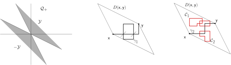
Figure 1. Positive quadrant $\mathcal{Q}_{+}$ and cones $\mathcal{Y}$, $-\mathcal{Y}$. Irreducible path $\gamma_{1}\subset D(\mathsf{x},\mathsf{y})$ and irreducible animal $[\gamma_{2},\mathcal{C}_{1},\mathcal{C}_{2}]$.

In its turn the notation $\mathfrak{A}_{\ell}$ stands for words of $\ell$ irreducible animals, and, in the latter case, we shall write $\underline{\Gamma}\in\mathfrak{A}_{\ell}$. By construction, such $\underline{\Gamma}$ is represented as $\underline{\Gamma}=[\underline{\gamma},\underline{\mathcal{C}}]$, where $\underline{\gamma}$ is a concatenation of letters from $\mathsf{P}$. The notation $\mathfrak{A}_{\ell}(\mathsf{x},\mathsf{y})$ stands for those elements of $\mathfrak{A}_{\ell}$ which have the left end-point at $\mathsf{x}$ and the right end point at $\mathsf{y}$. Finally, $\mathfrak{A}(\mathsf{x},\mathsf{y})\stackrel{{\scriptstyle\Delta}}{{=}}\cup_{\ell}\mathfrak{A}_{\ell}(\mathsf{x},\mathsf{y})$. In the case of animals the quantities $\left|\underline{\Gamma}\right|$, $\mathsf{X}(\underline{\Gamma})$ are defined through the corresponding path components. That is: $\left|[\gamma,\underline{\mathcal{C}}]\right|\stackrel{{\scriptstyle\Delta}}{{=}}\left|\gamma\right|$ and $\mathsf{X}\left([\gamma,\underline{\mathcal{C}}]\right)\stackrel{{\scriptstyle\Delta}}{{=}}\mathsf{X}(\gamma)$.

As discussed above we may restrict attention to those animals which contain at least $\delta^{\prime}\left|x\right|$ break points (for some $\delta^{\prime}>0$). This leads to the irreducible decomposition

$$[\gamma,\underline{\mathcal{C}}]=\Gamma^{[\mathsf{l}]}\circ\Gamma^{[1]}\circ\dots\circ\Gamma^{[n]}\circ\Gamma^{[\mathsf{r}]},$$ (4.9)

with $\Gamma^{[\mathsf{l}]}\in\mathsf{A}_{\mathsf{l}}$, $\Gamma^{[\mathsf{r}]}\in\mathsf{A}_{\mathsf{r}}$ and $\Gamma^{[1]},\dots,\Gamma^{[n]}\in\mathsf{A}$.

Input from Ornstein-Zernike (OZ) theory.

The relevant input from the OZ theory (see for instance Subsections 3.3 and 3.4 of [15]) could be summarized as follows:

Theorem 4.

For all $\beta$ large enough the surface tension $\tau_{\beta}$ in (3.4) is well defined and it is a support function of a convex set ${\mathbf{K}}_{\beta}$ with non-empty interior and locally analytic boundary $\partial{\mathbf{K}}_{\beta}$, which has a uniformly positive curvature. In particular $\tau_{\beta}$ is differentiable at any $\mathsf{x}\neq 0$ and $\mathsf{h}=\mathsf{h}_{\mathsf{x}}\stackrel{{\scriptstyle\Delta}}{{=}}\nabla\tau_{\beta}(\mathsf{x})\in\partial{\mathbf{K}}_{\beta}$. The Wulff shape ${\mathbf{K}}_{\beta}$ inherits the full set of $\mathbb{Z}^{2}$-lattice symmetries from the surface tension $\tau_{\beta}(\mathsf{x})$. In particular $\mathsf{h}_{\mathsf{x}}\in\mathcal{Q}_{+}$ whenever $\mathsf{x}\in\mathcal{Q}_{+}$. In geometric terms $\mathsf{h}_{\mathsf{x}}$ can be characterized in the following way: $\mathsf{x}$ is direction of the outward normal to $\partial{\mathbf{K}}_{\beta}$ at $\mathsf{h}_{\mathsf{x}}$. In view of smoothness and strict convexity of $\partial{\mathbf{K}}_{\beta}$ this is an unambiguous characterization.
For any $\mathsf{x}\in\mathcal{Q}_{+}\setminus 0$ the collection of weights

$$\mathbb{P}_{\beta}^{\mathsf{h}_{\mathsf{x}}}\left(\Gamma\right)\stackrel{{\scriptstyle\Delta}}{{=}}{\rm e}^{\mathsf{h}_{\mathsf{x}}\cdot\mathsf{X}(\Gamma)}q(\Gamma)$$ (4.10)

is a probability distribution on the set $\mathsf{A}$ of irreducible animals. The expectation $\mathsf{v}^{*}(\beta,\mathsf{x})$ of $\mathsf{X}(\Gamma)$ under $\mathbb{P}_{\beta}^{\mathsf{h}_{\mathsf{x}}}$ is collinear to $\mathsf{x}$: there exists $\alpha=\alpha(\beta,\mathsf{x})>0$ such that $\mathsf{v}^{*}(\beta,\mathsf{x})=\alpha\mathsf{x}$. Note that, since $\tau_{\beta}$ is homogeneous of order one, $\mathsf{v}^{*}(\beta,\mathsf{x})$ depends only on the direction of $\mathsf{x}$.

Furthermore, there exists a (mass-gap) constant $\nu_{\mathsf{g}}>0$, such that

$$\sum_{\Gamma\in\mathsf{A}_{\mathsf{l}}}\mathbb{P}_{\beta}^{\mathsf{h}_{\mathsf{x}}}(\Gamma){1\hskip-3.0pt\rm{I}}_{\left\{\left|\Gamma\right|\geq k\right\}}+\sum_{\Gamma\in\mathsf{A}_{\mathsf{r}}}\mathbb{P}_{\beta}^{\mathsf{h}_{\mathsf{x}}}(\Gamma){1\hskip-3.0pt\rm{I}}_{\left\{\left|\Gamma\right|\geq k\right\}}\leq c\,{\rm e}^{-\nu_{\mathsf{g}}\beta k},$$ (4.11)

uniformly in $\beta$ large, $\mathsf{x}\in\mathcal{Q}_{+}$ and $k>1$.

Remark 5.

In the sequel we shall sometimes employ an alternative notation $\mathsf{h}_{\epsilon}=\mathsf{h}_{\mathsf{x}}$ for $\mathsf{x}\in\mathcal{Q}_{+}$ satisfying $\frac{\mathsf{x}}{\left|\mathsf{x}\right|_{1}}=(1-\epsilon,\epsilon)$.

The target upper bound.

Let us fix (without loss of generality) $\mathsf{n}$ with ${\rm arg}(\mathsf{n})\in[\frac{\pi}{2},\frac{3\pi}{4}]$ and $\mathsf{x}\in\mathcal{B}_{+,\mathsf{n}}$. To facilitate notation set

$$\mathfrak{A}_{\ell}^{+,\mathsf{n}}=\mathfrak{A}_{\ell}\cap\left\{\underline{\Gamma}=[\underline{\gamma},\underline{\mathcal{C}}]:\underline{\gamma}\subset\mathcal{H}_{+,\mathsf{n}}\right\},$$ (4.12)

and, for any $\mathsf{u},\mathsf{v}\in\mathcal{H}_{+,\mathsf{n}}$, $\mathfrak{A}_{\ell}^{+,\mathsf{n}}(\mathsf{u},\mathsf{v})=\mathfrak{A}_{\ell}^{+,\mathsf{n}}\cap\left\{\underline{\Gamma}=[\underline{\gamma},\underline{\mathcal{C}}]:\underline{\gamma}:\mathsf{u}\mapsto\mathsf{v}\right\}$.

Recall that $\mathsf{h}=\mathsf{h}_{\mathsf{x}}=\nabla\tau_{\beta}(\mathsf{x})$ so that $\mathsf{h}\cdot\mathsf{x}=\tau_{\beta}(\mathsf{x})$. In view of (4.6) and (4.11), the two-point function $G_{\beta}^{+,\mathsf{n}}(\mathsf{x})$ is bounded above by

$${c_{1}(\beta)}\!\!\!\sum_{\begin{subarray}{c}\mathsf{u},\mathsf{x}-\mathsf{v}\in\mathcal{Y}\\ \mathsf{u},\mathsf{v}\in\mathcal{H}_{+,\mathsf{n}}\end{subarray}}{\rm e}^{-\nu_{\mathsf{g}}\beta\left(\left|\mathsf{u}\right|_{1}+\left|\mathsf{x}-\mathsf{v}\right|_{1}\right)}\sum_{\ell}\ \sum_{\underline{\Gamma}\in\mathfrak{A}_{\ell}^{+,\mathsf{n}}(\mathsf{u},\mathsf{v})}\mathbb{P}_{\beta}^{\mathsf{h}}\left(\underline{\Gamma}\right){\rm exp}\left\{\sum_{\mathsf{y}\in\underline{\gamma}}{\rm e}^{-\chi\beta({\rm d}_{\mathsf{n}}(\mathsf{y})+1)}\right\}.$$ (4.13)

We used that $\left|\mathsf{X}(\underline{\Gamma})\right|_{1}\leq\left|\underline{\Gamma}\right|$, where $|\mathsf{x}|_{1}$ is the $L^{1}$ norm of $\mathsf{x}$. Therefore, in order to derive the upper bound in (3.9), it suffices to check that there exists $0<{4}\delta<\nu_{\mathsf{g}}$ such that

$$\begin{split}&\sup_{\begin{subarray}{c}\mathsf{u},\mathsf{x}-\mathsf{v}\in\mathcal{Y}\\ \mathsf{u},\mathsf{v}\in\mathcal{H}_{+,\mathsf{n}}\end{subarray}}{\rm e}^{-{3}\delta\beta\left(\left|\mathsf{u}\right|_{1}+\left|\mathsf{x}-\mathsf{v}\right|_{1}\right)}\sum_{\ell}\ \sum_{\underline{\Gamma}\in\mathfrak{A}_{\ell}^{+,\mathsf{n}}(\mathsf{u},\mathsf{v})}\mathbb{P}_{\beta}^{\mathsf{h}}\left(\underline{\Gamma}\right){\rm exp}\Bigl{[}\sum_{\mathsf{y}\in\underline{\gamma}}{\rm e}^{-\chi\beta({\rm d}_{\mathsf{n}}(\mathsf{y})+1)}\Bigr{]}\\ &\qquad\qquad\leq c_{2}(\beta)\,G_{\beta}\left(\mathsf{x}\big{|}\mathcal{P}_{+,\mathsf{n}}\right){\rm e}^{\tau_{\beta}(\mathsf{x})}\end{split}$$ (4.14)

for $\beta$ sufficiently large, uniformly in $\mathsf{n}\in[\frac{\pi}{2},\frac{3\pi}{4}]$ and $\mathsf{x}\in\mathcal{B}_{+,\mathsf{n}}$.

5. Effective random walk

Steps of the effective random walk are displacements $\mathsf{X}(\Gamma)$ along irreducible animals $\Gamma$ which are sampled from the probability distribution (4.10). In this way the constraint $\underline{\gamma}\subset\mathcal{H}_{+,\mathsf{n}}$ is less stringent than the constraint that corresponding effective walk stays above the wall. In terms of effective random walks upper bounds on partition functions with pinning are given by quantities $\mathbb{G}^{\mathsf{h}}_{\beta,+}$ defined in (5.7). The corresponding effective random walk quantities for models without pinning are probabilities $\mathbb{P}_{\beta,+}^{\mathsf{h}}$ which are defined in (5.10). In the end of the Section we formulate Theorem 6 and explain how it implies our target upper bound (4.14) and, consequently, the upper bound in Theorem 2.

Random walk representation and high temperature expansion.

Let us reformulate the required bound in the effective random walk context: For a word $\underline{\Gamma}\in\mathfrak{A}_{\ell}$ with the left end point at $\mathsf{u}$ set

$$\mathsf{R}_{\ell}=\mathsf{R}_{\ell}(\underline{\Gamma})=\mathsf{u}+\sum_{i=1}^{\ell}\mathsf{X}(\gamma^{[i]})\stackrel{{\scriptstyle\Delta}}{{=}}\mathsf{u}+\sum_{i=1}^{\ell}\mathsf{X}_{i},$$ (5.1)

and, accordingly, define $Z_{i}=\mathsf{X}_{i}\cdot\mathsf{n}$ and

$$S_{\ell}=\mathsf{R}_{\ell}\cdot\mathsf{n}\ =\mathsf{u}\cdot\mathsf{n}+\sum_{i=1}^{n}\mathsf{X}_{i}\cdot\mathsf{n}=S_{0}+\sum_{1}^{\ell}Z_{i}.$$ (5.2)

For the random walk starting at $\mathsf{u}$ the probability $\mathbb{P}_{\beta}^{\mathsf{h}}\left(\mathsf{R}_{\ell}=\mathsf{v}\right)=\mathbb{P}_{\beta}^{\mathsf{h}}\left(\mathfrak{A}_{\ell}(\mathsf{u},\mathsf{v})\right)$.

Define events (sets of words)

$$\mathfrak{R}_{\ell}^{+,\mathsf{n}}=\mathfrak{R}_{\ell}^{+}=\left\{\underline{\Gamma}\in\mathfrak{A}_{\ell}:\,S_{1},\dots,S_{\ell-1}\geq 0\right\}.$$ (5.3)

With a slight abuse of notation we shall think of $\mathfrak{R}_{\ell}^{+}$ both as a subset of $\mathfrak{A}_{\ell}$ and as a subset of $\mathfrak{A}_{m}$ for any $\ell\leq m\leq\infty$. The notation $\mathfrak{R}_{\ell}^{+}(\mathsf{u},\mathsf{v})$ stands for $\ell$-strings of irreducible animals from $\mathfrak{R}_{\ell}^{+}$ with the left end point at $\mathsf{u}$ and the right end point at $\mathsf{v}$; $\mathfrak{R}_{\ell}^{+}(\mathsf{u},\mathsf{v})=\mathfrak{R}_{\ell}^{+}\cap\mathfrak{A}\left(\mathsf{u},\mathsf{v}\right)$. Note that $\mathfrak{A}_{\ell}^{+}(\mathsf{u},\mathsf{v})\subseteq\mathfrak{R}_{\ell}^{+}(\mathsf{u},\mathsf{v})$.

Given a string $\underline{\Gamma}$ define (recall the definition (4.8) of diamond shapes): $D_{\ell}=D(\mathsf{R}_{\ell-1},\mathsf{R}_{\ell})$. By construction, $\Gamma^{[\ell]}\subset D_{\ell}$. Next define $d_{\ell}\stackrel{{\scriptstyle\Delta}}{{=}}d(\mathsf{R}_{\ell-1},\mathsf{R}_{\ell})\geq 0$ via

$$d_{\ell}=d(\mathsf{R}_{\ell-1},\mathsf{R}_{\ell})=\min_{\mathsf{y}\in D_{\ell}\cap\mathcal{H}_{+,\mathsf{n}}\cap\mathbb{Z}_{*}^{2}}\left({\rm d}_{\mathsf{n}}(\mathsf{y})+1\right)-2\geq 0.$$ (5.4)

For strings $\underline{\Gamma}\in\mathfrak{A}_{n}^{+}(\mathsf{u},\mathsf{v})$ the contour part $\gamma^{[\ell]}$ of the $\ell$-th irreducible animal $\Gamma^{[\ell]}$ satisfies:

$$\sum_{\mathsf{y}\in\gamma^{[\ell]}}{\rm e}^{-\chi\beta({\rm d}_{\mathsf{n}}(\mathsf{y})+1)}\leq\left|\gamma^{[\ell]}\right|{\rm e}^{-\chi\beta(2+d_{\ell})}\stackrel{{\scriptstyle\Delta}}{{=}}\phi_{\beta}(\gamma^{[\ell]}).$$ (5.5)

Note that the weight $\phi_{\beta}(\gamma^{[\ell]})$ just defined can be quite large. But this will be compensated by the fact that the probability $\mathbb{P}_{\beta}^{\mathsf{h}}\left(\Gamma^{[\ell]}\right)$ of the corresponding animal $\Gamma^{[\ell]}$ is very small.

By (5.5),

$$\sum_{\underline{\Gamma}\in\mathfrak{A}_{\ell}^{+,\mathsf{n}}(\mathsf{u},\mathsf{v})}\mathbb{P}_{\beta}^{\mathsf{h}}\left(\underline{\Gamma}\right){\rm exp}\left\{\sum_{\mathsf{y}\in\underline{\gamma}}{\rm e}^{-\chi\beta({\rm d}_{\mathsf{n}}(\mathsf{y})+1)}\right\}\leq\sum_{\underline{\Gamma}\in\mathfrak{R}_{\ell}^{+,\mathsf{n}}(\mathsf{u},\mathsf{v})}\mathbb{P}_{\beta}^{\mathsf{h}}\left(\underline{\Gamma}\right)\prod_{j=1}^{\ell}e^{\phi_{\beta}(\gamma^{[j]})}$$ (5.6)

for any $\ell=1,2,3\dots$. Define

$${\mathbb{G}^{\mathsf{h}}_{\beta,+}(\mathsf{u},\mathsf{v})}=\sum_{\ell}\ \sum_{\underline{\Gamma}\in\mathfrak{R}_{\ell}^{+,\mathsf{n}}(\mathsf{u},\mathsf{v})}\mathbb{P}_{\beta}^{\mathsf{h}}\left(\underline{\Gamma}\right)\prod_{i=1}^{\ell}{\rm e}^{\phi_{\beta}(\gamma^{[i]})}.$$ (5.7)

We conclude that

$$\text{ left hand side of \eqref{eq:Target1}}\leq\sup_{\begin{subarray}{c}\mathsf{u},\mathsf{x}-\mathsf{v}\in\mathcal{Y}\\ \mathsf{u},\mathsf{v}\in\mathcal{H}_{+,\mathsf{n}}\end{subarray}}{\rm e}^{-{3}\delta\beta\left(\left|\mathsf{u}\right|_{1}+\left|\mathsf{x}-\mathsf{v}\right|_{1}\right)}\mathbb{G}^{\mathsf{h}}_{\beta,+}(\mathsf{u},\mathsf{v}).$$ (5.8)

Observe that

$$|\mathsf{u}|_{1}+|\mathsf{v}-\mathsf{x}|_{1}\geq{\rm d}_{\mathsf{n}}(\mathsf{u})+{\rm d}_{\mathsf{n}}(\mathsf{v}){-2},$$ (5.9)

if $\mathsf{u},\mathsf{x}-\mathsf{v}\in\mathcal{Y}$ and $\mathsf{u},\mathsf{v}\in\mathcal{H}_{+,\mathsf{n}}$.

With (5.8) and (5.9) in mind define:

$$\mathbb{P}_{\beta,+}^{\mathsf{h}}(\mathsf{u},\mathsf{v})=\sum_{\ell}\mathbb{P}_{\beta}^{\mathsf{h}}\left(\mathfrak{R}_{\ell}^{+,\mathsf{n}}(\mathsf{u},\mathsf{v})\right)\ {\rm and}\ \rho_{\delta}(\mathsf{u},\mathsf{v})=\frac{{\rm e}^{-\delta\beta{\rm d}_{\mathsf{n}}(\mathsf{u})}\mathbb{G}^{\mathsf{h}}_{\beta,+}(\mathsf{u},\mathsf{v}){\rm e}^{-\delta\beta{\rm d}_{\mathsf{n}}(\mathsf{v})}}{{\rm e}^{\delta\beta{\rm d}_{\mathsf{n}}(\mathsf{u})}\mathbb{P}_{\beta,+}^{\mathsf{h}}\left(\mathsf{u},\mathsf{v}\right){\rm e}^{\delta\beta{\rm d}_{\mathsf{n}}(\mathsf{v})}.}.$$ (5.10)

Then, (4.14) and hence the upper bound of Theorem 2 are consequence of:

Theorem 6.

There exist $0<\delta<\nu_{\mathsf{g}}/4$ and $\beta_{0}$ sufficiently large such that the following holds: For any $\beta>\beta_{0}$ there exists a constant $c=c(\beta)$, such that

1. uniformly in ${\rm arg}\left(\mathsf{n}\right)\in\left[\frac{\pi}{2},\frac{3\pi}{4}\right]$ and in all $\mathsf{u},\mathsf{v}\in\mathcal{H}_{+,\mathsf{n}}$, $\mathsf{u},\mathsf{x}-\mathsf{v}\in\mathcal{Y}$,

   $$\rho_{\delta}(\mathsf{u},\mathsf{v})\leq c(\beta).$$ (5.11)

2. uniformly in $\mathsf{x}\in\mathcal{B}_{+,\mathsf{n}}$,

   $$\sup_{\begin{subarray}{c}\mathsf{u},\mathsf{x}-\mathsf{v}\in\mathcal{Y}\\ \mathsf{u},\mathsf{v}\in\mathcal{H}_{+,\mathsf{n}}\end{subarray}}{\rm e}^{-\delta\beta\left(\left|\mathsf{u}\right|_{1}+\left|\mathsf{x}-\mathsf{v}\right|_{1}\right)}\mathbb{P}_{\beta,+}^{\mathsf{h}_{\mathsf{x}}}(\mathsf{u},\mathsf{v})\leq c(\beta)\,G_{\beta}\left(\mathsf{x}\big{|}\mathcal{P}_{+,\mathsf{n}}\right)e^{\tau_{\beta}(\mathsf{x})}.$$ (5.12)

Claim (B) is an expression of entropic repulsion, and it has the same flavour as the lower bound of Theorem 2. We prove both in Subsection 6.2.

In order to see how (A) and (B) imply our target upper bound (4.14) notice that

$$\begin{split}&{\rm e}^{-{3}\delta\beta\left(\left|\mathsf{u}\right|_{1}+\left|\mathsf{x}-\mathsf{v}\right|_{1}\right)}\mathbb{G}^{\mathsf{h}}_{\beta,+}(\mathsf{u},\mathsf{v})\leq\rho_{\delta}(\mathsf{u},\mathsf{v}){{\rm e}^{4\delta\beta}}{\rm e}^{-\delta\beta\left(\left|\mathsf{u}\right|_{1}+\left|\mathsf{x}-\mathsf{v}\right|_{1}\right)}\mathbb{P}_{\beta,+}^{\mathsf{h}_{\mathsf{x}}}(\mathsf{u},\mathsf{v})\\ &\qquad\stackrel{{\scriptstyle\eqref{eq:TwoBounds1},\eqref{eq:TwoBounds2}}}{{\leq}}c(\beta)^{2}{{\rm e}^{4\delta\beta}}\,G_{\beta}\left(\mathsf{x}\big{|}\mathcal{P}_{+,\mathsf{n}}\right)e^{\tau_{\beta}(\mathsf{x})}{\stackrel{{\scriptstyle\Delta}}{{=}}c_{2}(\beta)G_{\beta}\left(\mathsf{x}\big{|}\mathcal{P}_{+,\mathsf{n}}\right)e^{\tau_{\beta}(\mathsf{x})}},\end{split}$$ (5.13)

where the first inequality follows from (5.9) and from the very definition of $\rho_{\delta}$ in (5.10), whereas the second inequality is precisely (5.11) and (5.12). The target bound (4.14) follows from (5.13) because of (5.8). ∎

6. Proof of Theorem 6 and the lower bound of Theorem 2

In this Section we prove Theorem 6 and the lower bound in Theorem 2. Claim (A) of Theorem 6 is the most difficult part and the arguments hinge upon crucial estimates of Proposition 11. The proof of the latter is relegated to Section 8. Claim (B) of Theorem 6 and of the lower bound in Theorem 2 are somewhat simpler statements. The proof is based on Proposition 12 (which is in its turn proved in Section 8) and, in the very end - see (6.37), on Proposition 11.

The impact of the pinning potential is encoded in the recursion (6.4), which, by taking maxima, leads to the uniform recursion (6.17). Proposition 11 ensures that (6.17) implies Claim (A) of Theorem 6. In Section 8 decay properties (6.11) of potential $\Psi_{\beta}^{\mathsf{h},\delta}$ play an important role in the proof of Proposition 11.

Claim (B) of Theorem 6 and the lower bound of Theorem 2 are statements about entropic repulsion of the effective random walk away from $\mathcal{B}_{+,\mathsf{n}}$. Our approach is based on [3]. Key facts along these lines are formulated in Proposition 13. Claim (B) of Theorem 6 (in the form of (6.25)) and lower bound of Theorem 2 (in the form of (6.26)) are easy consequences. The proof of Proposition 12, which gives an upper bound on the left hand side of (5.12) in terms of $\mathbb{P}_{\beta,+}^{\mathsf{h}_{\mathsf{x}}}(0,\mathsf{x})$, is relegated to Subsection 8.3.

6.1. Claim (A)

Let us start by making one remark:

Remark 7.

By the first of (4.5) and by the crude upper bound (4.6)

$$\log\rho_{\delta}(\mathsf{u},\mathsf{v})\leq r_{0}\left|\mathsf{v}-\mathsf{u}\right|_{1}{\rm e}^{-{2}\chi\beta}-2\delta\beta\left({\rm d}_{\mathsf{n}}(\mathsf{u})+{\rm d}_{\mathsf{n}}(\mathsf{v})\right),$$

which means that $\rho_{\delta}(\mathsf{u},\mathsf{v})\leq 1$ unless $\mathsf{u}$ and $\mathsf{v}$ stay appropriately close to $\mathcal{B}_{+,\mathsf{n}}$ in the sense that the pair $\left(\mathsf{u},\mathsf{v}\right)\in\mathcal{A}$, where

$$\mathcal{A}\stackrel{{\scriptstyle\Delta}}{{=}}\left\{(\mathsf{u},\mathsf{v}):\,{\mathsf{u},\mathsf{x}-\mathsf{v}\in\mathcal{Y}},{\mathsf{u},\mathsf{v}\in\mathcal{H}_{+,\mathsf{n}}},{\rm d}_{\mathsf{n}}(\mathsf{u})+{\rm d}_{\mathsf{n}}(\mathsf{v})\leq\frac{r_{0}{\rm e}^{-{2}\chi\beta}}{{2}\delta\beta}\left|\mathsf{v}-\mathsf{u}\right|_{1}\right\}.$$ (6.1)

In particular, since $\chi>\frac{1}{2}$, we may assume that there exists $\nu>1$ such that

$$|\mathsf{v}-\mathsf{u}|_{1}\geq\left({\rm d}_{\mathsf{n}}(\mathsf{u})+{\rm d}_{\mathsf{n}}(\mathsf{v})\right){\rm e}^{\nu\beta}\quad\text{and}\quad|\arg(\mathsf{v}-\mathsf{u})-\arg(\mathsf{n}^{\perp})|\leq{\rm e}^{-\nu\beta},$$ (6.2)

where $\mathsf{n}^{\perp}\stackrel{{\scriptstyle\Delta}}{{=}}(n_{2},-n_{1})$. There is no loss of generality (otherwise we would just consider the reversed walk) to assume that $\mathsf{n}\cdot(\mathsf{v}-\mathsf{u})\geq 0$. This ensures that the drift $\mathsf{h}=\nabla\tau_{\beta}(\mathsf{v}-\mathsf{u})$ has non-negative entries.

∎

The proof of the claim A comprises several steps.

STEP 1 (Recursion) Manipulating expansions of

$$\prod_{i=1}^{\ell}{\rm e}^{\phi_{\beta}(\gamma^{[i]})}=\prod_{i=1}^{\ell}\left(1+\left({\rm e}^{\phi_{\beta}(\gamma^{[i]})}-1\right)\right),$$ (6.3)

we infer that

$$\begin{split}&\mathbb{G}^{\mathsf{h}}_{\beta,+}(\mathsf{u},\mathsf{v})=\mathbb{P}_{\beta,+}^{\mathsf{h}}(\mathsf{u},\mathsf{v})+\sum_{\mathsf{w},\mathsf{z}}\mathbb{P}_{\beta,+}^{\mathsf{h}}(\mathsf{u},\mathsf{w})\Phi_{\beta,+}^{\mathsf{h}}(\mathsf{w},\mathsf{z})\mathbb{P}_{\beta,+}^{\mathsf{h}}(\mathsf{z},\mathsf{v})\\ &+\quad\sum_{\mathsf{w}_{1},\mathsf{z}_{1}}\sum_{\mathsf{w}_{2},\mathsf{z}_{2}}\mathbb{P}_{\beta,+}^{\mathsf{h}}(\mathsf{u},\mathsf{w}_{1})\Phi_{\beta}^{\mathsf{h}}(\mathsf{w}_{1},\mathsf{z}_{1})\mathbb{G}^{\mathsf{h}}_{\beta,+}(\mathsf{z}_{1},\mathsf{w}_{2})\Phi_{\beta}^{\mathsf{h}}(\mathsf{w}_{2},\mathsf{z}_{2})\mathbb{P}_{\beta,+}^{\mathsf{h}}(\mathsf{z}_{2},\mathsf{v}),\end{split}$$ (6.4)

where we have defined:

$$\Phi_{\beta}^{\mathsf{h}}(\mathsf{w},\mathsf{z})=\mathbb{E}_{\beta}^{\mathsf{h}}\left({1\hskip-3.0pt\rm{I}}_{\mathsf{A}(\mathsf{w},\mathsf{z})}\left({\rm e}^{\phi_{\beta}(\gamma)}-1\right)\right).$$ (6.5)

Equation (6.4) gives rise to the following recursion: Set

$$\begin{split}\underline{\mathbb{P}}_{\beta,+}^{\mathsf{h},\delta}(\mathsf{s},\mathsf{t})&={\rm e}^{-\delta\beta{\rm d}_{\mathsf{n}}(\mathsf{s})}{\mathbb{P}}_{\beta,+}^{\mathsf{h}}(\mathsf{s},\mathsf{t}){\rm e}^{-\delta\beta{\rm d}_{\mathsf{n}}(\mathsf{t})},\\ \bar{\mathbb{P}}_{\beta,+}^{\mathsf{h},\delta}(\mathsf{u},\mathsf{v})&={\rm e}^{\delta\beta{\rm d}_{\mathsf{n}}(\mathsf{u})}{\mathbb{P}}_{\beta,+}^{\mathsf{h}}(\mathsf{u},\mathsf{v}){{\rm e}^{\delta\beta{\rm d}_{\mathsf{n}}(\mathsf{v})}}\end{split}$$ (6.6)

and

$$\Psi_{\beta}^{\mathsf{h},\delta}(\mathsf{w},\mathsf{z})={\rm e}^{3\delta\beta{\rm d}_{\mathsf{n}}(\mathsf{w})}\Phi_{\beta}^{\mathsf{h}}(\mathsf{w},\mathsf{z}){\rm e}^{3\delta\beta{\rm d}_{\mathsf{n}}(\mathsf{z})}.$$ (6.7)

With this notation (6.4) and (5.10) imply:

$$\begin{split}&\rho_{\delta}(\mathsf{u},\mathsf{v})\leq{\rm e}^{-2\delta\beta\left({\rm d}_{\mathsf{n}}(\mathsf{u})+{\rm d}_{\mathsf{n}}(\mathsf{v})\right)}+\sum_{\mathsf{w},\mathsf{z}}\frac{\underline{\mathbb{P}}_{\beta,+}^{\mathsf{h},\delta}(\mathsf{u},\mathsf{w})\Psi_{\beta}^{\mathsf{h},\delta}(\mathsf{w},\mathsf{z})\underline{\mathbb{P}}_{\beta,+}^{\mathsf{h},\delta}(\mathsf{z},\mathsf{v})}{\bar{\mathbb{P}}_{\beta,+}^{\mathsf{h},\delta}(\mathsf{u},\mathsf{v})}\\ &+\sum_{\mathsf{w}_{1},\mathsf{z}_{1}}\sum_{\mathsf{w}_{2},\mathsf{z}_{2}}\frac{\underline{\mathbb{P}}_{\beta,+}^{\mathsf{h},\delta}(\mathsf{u},\mathsf{w}_{1})\Psi_{\beta}^{\mathsf{h},\delta}(\mathsf{w}_{1},\mathsf{z}_{1})\underline{\mathbb{P}}_{\beta,+}^{\mathsf{h},\delta}(\mathsf{z}_{1},\mathsf{w}_{2})\Psi_{\beta}^{\mathsf{h},\delta}(\mathsf{w}_{2},\mathsf{z}_{2})\underline{\mathbb{P}}_{\beta,+}^{\mathsf{h},\delta}(\mathsf{z}_{2},\mathsf{v})}{\bar{\mathbb{P}}_{\beta,+}^{\mathsf{h},\delta}(\mathsf{u},\mathsf{v})}\rho_{\delta}(\mathsf{z}_{1},\mathsf{w}_{2}).\end{split}$$ (6.8)

Remark 8.

None of the ratios in (6.8) depends on the drift $\mathsf{h}$. It will be convenient to take $\mathsf{h}=\nabla\tau_{\beta}(\mathsf{v}-\mathsf{u})$.

STEP 2 (Bounds on $\Psi_{\beta}^{\mathsf{h},\delta}$) Recall the definition of the weights $\phi_{\beta}$ in (5.5). Then,

$$\Psi_{\beta}^{\mathsf{h},\delta}(\mathsf{w},\mathsf{z}){\,=\,}{\rm e}^{3\delta\beta{\rm d}_{\mathsf{n}}(\mathsf{w})}\mathbb{E}_{\beta}^{\mathsf{h}}{1\hskip-3.0pt\rm{I}}_{\mathsf{A}(\mathsf{w},\mathsf{z})}\left({\rm exp}\left(\left|\gamma\right|{\rm e}^{-\beta\chi\left(2+d(\mathsf{w},\mathsf{z})\right)}\right)-1\right){\rm e}^{3\delta\beta{\rm d}_{\mathsf{n}}(\mathsf{z})},$$ (6.9)

where the function $d(\mathsf{w},\mathsf{z})\geq 0$ was already defined in (5.4):

$$d(\mathsf{w},\mathsf{z})=\min_{\mathsf{y}\in D(\mathsf{w},\mathsf{z})\cap\mathcal{H}_{+,\mathsf{n}}\cap\mathbb{Z}_{*}^{2}}\left({\rm d}_{\mathsf{n}}(\mathsf{y})+1\right)-2.$$ (6.10)

Lemma 9.

There exist $\nu_{2},\nu_{3}>0$ and $c_{1},R<\infty$ such that for any $\chi^{\prime}<\chi$ one can choose $\delta_{0}>0$, such that, uniformly in $\delta\leq\delta_{0}$, admissible pairs $\left\{\left(\mathsf{w},\mathsf{z}\right):\mathsf{z}\in\mathsf{w}+\mathcal{Y}\right\}$ and $\beta$ large, the following holds:

$$\Psi_{\beta,\delta}^{\mathsf{h}}(\mathsf{w},\mathsf{z})\leq c_{1}\,{\rm e}^{-2\chi^{\prime}\beta}\mathcal{K}_{\beta}(\mathsf{w},\mathsf{z}),$$ (6.11)

where the kernel $\mathcal{K}_{\beta}$ is given by

$$\mathcal{K}_{\beta}(\mathsf{w},\mathsf{z})=\exp\left[{-\nu_{3}\beta\left({\rm d}_{\mathsf{n}}(\mathsf{w})-R\right)_{+}}{-\nu_{2}\beta\left|\mathsf{z}-\mathsf{w}\right|_{1}{1\hskip-3.0pt\rm{I}}_{\left|\mathsf{z}-\mathsf{w}\right|_{1}>1}}{-\nu_{3}\beta\left({\rm d}_{\mathsf{n}}(\mathsf{z})-R\right)_{+}}\right].$$ (6.12)

Remark 10.

Lemma  states that $\Psi_{\beta,\delta}^{\mathsf{h}}(\mathsf{w},\mathsf{z})$ is at most of order $\exp(-2\chi^{\prime}\beta)$ and that the kernel $\mathcal{K}_{\beta}(\mathsf{w},\mathsf{z})$ decays exponentially both in $|\mathsf{z}-\mathsf{w}|_{1}$ and in the distances ${\rm d}_{\mathsf{n}}(\mathsf{w}),{\rm d}_{\mathsf{n}}(\mathsf{z})$ from the wall. In particular, $\sum_{\mathsf{w},\mathsf{z}}\mathcal{K}_{\beta}(\mathsf{w},\mathsf{z})$ is essentially a one dimensional sum over lattice points inside a strip of width $R$ along $\partial\mathcal{H}_{+,\mathsf{n}}$.

Proof of Lemma 9

By construction of diamond shapes there exists $\alpha\in\mathbb{N}$, such that

$$d(\mathsf{w},\mathsf{z})\geq\frac{1}{2}\left(\left({\rm d}_{\mathsf{n}}(\mathsf{z})-\alpha|\mathsf{w}-\mathsf{z}|_{1}\right)_{+}+\left({\rm d}_{\mathsf{n}}(\mathsf{w})-\alpha|\mathsf{w}-\mathsf{z}|_{1}\right)_{+}\right).$$ (6.13)

Above $a_{+}\stackrel{{\scriptstyle\Delta}}{{=}}a\vee 0$. To facilitate notation set

$$f_{\mathsf{w}\mathsf{z}}(k)=k{\rm e}^{-2\chi\beta-\frac{\chi\beta}{2}\left(\left({\rm d}_{\mathsf{n}}(\mathsf{z})-\alpha|\mathsf{w}-\mathsf{z}|_{1}\right)_{+}+\left({\rm d}_{\mathsf{n}}(\mathsf{w})-\alpha|\mathsf{w}-\mathsf{z}|_{1}\right)_{+}\right)}$$ (6.14)

Since $\left|\mathsf{X}(\gamma)\right|\leq\left|\gamma\right|$, and in view of (6.13),

$$\begin{split}\Psi_{\beta,\delta}^{\mathsf{h}}(\mathsf{w},\mathsf{z})&\leq{\rm e}^{3\delta\beta\left({\rm d}_{\mathsf{n}}(\mathsf{w})+{\rm d}_{\mathsf{n}}(\mathsf{z})\right)}\sum_{k\geq\left|\mathsf{z}-\mathsf{w}\right|_{1}}\left({\rm e}^{f_{\mathsf{w}\mathsf{z}}(k)}-1\right)\mathbb{P}_{\beta}^{\mathsf{h}}\left(\left|\gamma\right|=k\right)\\ &\ \ \leq{\rm e}^{3\delta\beta\left({\rm d}_{\mathsf{n}}(\mathsf{w})+{\rm d}_{\mathsf{n}}(\mathsf{z})\right)}\sum_{k\geq\left|\mathsf{z}-\mathsf{w}\right|_{1}}f_{\mathsf{w}\mathsf{z}}(k){\rm e}^{f_{\mathsf{w}\mathsf{z}}(k)}\mathbb{P}_{\beta}^{\mathsf{h}}\left(\left|\gamma\right|=k\right)\\ &\ \ \leq{\rm e}^{3\delta\beta\left({\rm d}_{\mathsf{n}}(\mathsf{w})+{\rm d}_{\mathsf{n}}(\mathsf{z})\right)}\sum_{k\geq\left|\mathsf{z}-\mathsf{w}\right|_{1}}f_{\mathsf{w}\mathsf{z}}(k){\rm e}^{f_{\mathsf{w}\mathsf{z}}(k)-2\nu_{\mathsf{g}}\beta k{1\hskip-3.0pt\rm{I}}_{k>1}}\\ &\ \ \leq 2{\rm e}^{3\delta\beta\left({\rm d}_{\mathsf{n}}(\mathsf{w})+{\rm d}_{\mathsf{n}}(\mathsf{z})\right)}\sum_{k\geq\left|\mathsf{z}-\mathsf{w}\right|_{1}}f_{\mathsf{w}\mathsf{z}}(k){\rm e}^{-\nu_{\mathsf{g}}\beta k{1\hskip-3.0pt\rm{I}}_{k>1}}.\end{split}$$ (6.15)

In the last two inequalities we relied on (4.11) and on (6.14).

Let us take a closer look at the definition (6.14) on $f_{\mathsf{w}\mathsf{z}}(k)$. Recall that $\alpha,\nu_{\mathsf{g}}$ and $\chi$ are positive constants which do not depend of $\beta$. Fix $\chi^{\prime}<\chi$ and $R>2\alpha$. Then, one can choose $\nu_{2},\nu_{3}>0$ and $\delta_{0}>0$ so small, so that for any $\delta\leq\delta_{0}$ and for any non-negative numbers $a,b\geq 0$,

$$\begin{split}&\nu_{\mathsf{g}}k{1\hskip-3.0pt\rm{I}}_{k>1}+2\chi+\frac{\chi}{2}\left(\left(a-\alpha k\right)_{+}+\left(b-\alpha k\right)_{+}\right)-3\delta a{-3\delta b}\\ &\quad\geq\nu_{2}k{1\hskip-3.0pt\rm{I}}_{k>1}+2\chi^{\prime}+\nu_{3}\left(\left(a-R\right)_{+}+\left(b-R\right)_{+}\right).\end{split}$$ (6.16)

Hence (6.11).∎

STEP 3 (Substitution and analysis of the Recursion (6.8)) As we noted in Remark 7 $\rho_{\delta}(\mathsf{u},\mathsf{v})\leq{1}$ for $\left(\mathsf{u},\mathsf{v}\right)\not\in\mathcal{A}$. Define

$$\rho_{\delta}=\max\{\sup_{(\mathsf{u},\mathsf{v})\in\mathcal{A}}\rho_{\delta}(\mathsf{u},\mathsf{v}),{1}\}.$$

Then (6.8) implies

$$\rho_{\delta}\leq 1+a_{\delta}+b_{\delta}\rho_{\delta},$$ (6.17)

where

$$a_{\delta}=\sup_{\left(\mathsf{u},\mathsf{v}\right)\in\mathcal{A}}\sum_{\mathsf{w},\mathsf{z}}\frac{\underline{\mathbb{P}}_{\beta,+}^{\mathsf{h},\delta}(\mathsf{u},\mathsf{w})\Psi_{\beta}^{\mathsf{h},\delta}(\mathsf{w},\mathsf{z})\underline{\mathbb{P}}_{\beta,+}^{\mathsf{h},\delta}(\mathsf{z},\mathsf{v})}{\bar{\mathbb{P}}_{\beta,+}^{\mathsf{h},\delta}(\mathsf{u},\mathsf{v})},$$ (6.18)

and, accordingly,

$$b_{\delta}=\sup_{\left(\mathsf{u},\mathsf{v}\right)\in\mathcal{A}}\sum_{\mathsf{w}_{1},\mathsf{z}_{1}}\sum_{\mathsf{w}_{2},\mathsf{z}_{2}}\frac{\underline{\mathbb{P}}_{\beta,+}^{\mathsf{h},\delta}(\mathsf{u},\mathsf{w}_{1})\Psi_{\beta}^{\mathsf{h},\delta}(\mathsf{w}_{1},\mathsf{z}_{1})\underline{\mathbb{P}}_{\beta,+}^{\mathsf{h},\delta}(\mathsf{z}_{1},\mathsf{w}_{2})\Psi_{\beta}^{\mathsf{h},\delta}(\mathsf{w}_{2},\mathsf{z}_{2})\underline{\mathbb{P}}_{\beta,+}^{\mathsf{h},\delta}(\mathsf{z}_{2},\mathsf{v})}{\bar{\mathbb{P}}_{\beta,+}^{\mathsf{h},\delta}(\mathsf{u},\mathsf{v})}.$$ (6.19)

Our target bound (5.11) follows then from (6.17) and:

Proposition 11.

Fix $\delta>0$. Then

$$a_{\delta}<\infty\ {\rm and}\ b_{\delta}<1,$$ (6.20)

uniformly in $\mathsf{n}\in\left[\frac{\pi}{2},\frac{3\pi}{4}\right]$, in all $\left(\mathsf{u},\mathsf{v}\right)$ satisfying (6.2) and in all $\beta$ sufficiently large.

We prove Proposition 11 in Section 8.

6.2. Claim (B) of Theorem 6 and the lower bound in Theorem 2

First of all we may consider $\mathbb{P}_{\beta,+}^{\mathsf{h}_{\mathsf{x}}}(0,\mathsf{x})$ instead of the left hand side in (5.12). The proof of the following Proposition is relegated to Subsection 8.3:

Proposition 12.

There exists $c_{1}=c_{1}(\beta)$ such that:

$$\max\left\{{\rm e}^{-\nu_{\mathsf{g}}\beta\left|\mathsf{x}\right|_{{1}}},\sup_{\begin{subarray}{c}\mathsf{u},\mathsf{x}-\mathsf{v}\in\mathcal{Y}\\ \mathsf{u},\mathsf{v}\in\mathcal{H}_{+,\mathsf{n}}\end{subarray}}{\rm e}^{-\delta\beta\left(\left|\mathsf{u}\right|_{1}+\left|\mathsf{x}-\mathsf{v}\right|_{1}\right)}\mathbb{P}_{\beta,+}^{\mathsf{h}_{\mathsf{x}}}(\mathsf{u},\mathsf{v})\right\}(\mathsf{u},\mathsf{v})\leq c_{1}\mathbb{P}_{\beta,+}^{\mathsf{h}_{\mathsf{x}}}(0,\mathsf{x}).$$ (6.21)

Thus, lower bounds for both $G_{\beta}\left(\mathsf{x}\big{|}\mathcal{P}_{+,\mathsf{n}}\right)$ and $G_{\beta}^{+\mathsf{n}}(\mathsf{x})$ may be derived in terms of $\mathbb{P}_{\beta,+}^{\mathsf{h}_{\mathsf{x}}}(0,\mathsf{x})$.

Given a string $\underline{\Gamma}=\left[\underline{\gamma},\underline{\mathcal{C}}\right]$ of irreducible animals, let us define (see (5.5))

$$F(\underline{\Gamma})=F(\underline{\gamma})=\sum_{\ell}\left|\gamma^{[\ell]}\right|{\rm e}^{-\beta\chi(d_{\ell}+2)}=\sum_{\ell}\phi_{\beta}(\gamma^{[\ell]}).$$ (6.22)

Both (5.12) and the lower bound in (3.9) are consequences of the following proposition:

Proposition 13.

For any $\beta\geq\beta_{0}$ there exist two constants $p_{\beta}>0$ and $K_{\beta}<\infty$ such that the following two bounds hold uniformly in ${\rm arg}(\mathsf{n})\in\left[\frac{\pi}{2},\frac{3\pi}{4}\right]$ and $\mathsf{x}\in\mathcal{B}_{+,\mathsf{n}}$:

$$\mathbb{P}_{\beta}^{\mathsf{h}_{\mathsf{x}}}\left(\mathfrak{A}^{+,\mathsf{n}}(0,\mathsf{x})~{}\Big{|}~{}\mathfrak{R}^{+,\mathsf{n}}(0,\mathsf{x})\right)=\frac{\mathbb{P}_{\beta}^{\mathsf{h}_{\mathsf{x}}}\left(\mathfrak{A}^{+,\mathsf{n}}(0,\mathsf{x})\right)}{\mathbb{P}_{\beta,+}^{\mathsf{h}_{\mathsf{x}}}\left(0,\mathsf{x}\right)}\geq p_{\beta},$$ (6.23)

and,

$$\mathbb{E}_{\beta}^{\mathsf{h}_{\mathsf{x}}}\left(F(\underline{\gamma})~{}\Big{|}~{}\mathfrak{R}^{+,\mathsf{n}}(0,\mathsf{x})\right)\leq K_{\beta}.$$ (6.24)

Before proving Proposition 13 let us demonstrate how it implies lower bounds in question:

Consider first (5.12). By (6.21) it would be enough to check that there exists a constant $c_{2}=c_{2}(\beta)$ such that

$$\mathbb{P}_{\beta,+}^{\mathsf{h}_{\mathsf{x}}}(0,\mathsf{x})\leq c_{2}\,G_{\beta}\left(\mathsf{x}\big{|}\mathcal{P}_{+,\mathsf{n}}\right)e^{\tau_{\beta}(\mathsf{x})}.$$ (6.25)

However,

$$G_{\beta}\left(\mathsf{x}\big{|}\mathcal{P}_{+,\mathsf{n}}\right)e^{\tau_{\beta}(\mathsf{x})}\geq\mathbb{P}_{\beta}^{\mathsf{h}_{\mathsf{x}}}\left(\mathfrak{A}^{+,\mathsf{n}}(0,\mathsf{x})\right).$$

Indeed, the right hand side above is just a restricted sum over animals with empty boundary pieces in the irreducible decomposition (4.9). By (6.23)

$$\mathbb{P}_{\beta}^{\mathsf{h}_{\mathsf{x}}}\left(\mathfrak{A}^{+,\mathsf{n}}(0,\mathsf{x})\right)\geq p_{\beta}\mathbb{P}_{\beta}^{\mathsf{h}_{\mathsf{x}}}\left(\mathfrak{R}^{+,\mathsf{n}}(0,\mathsf{x})\right)=p_{\beta}\mathbb{P}_{\beta,+}^{\mathsf{h}_{\mathsf{x}}}(0,\mathsf{x}),$$

and (6.25) follows.

Turning to the lower bound in (3.9) note that by (4.6)

$${\rm e}^{\tau_{\beta}(\mathsf{x})}G_{\beta}^{+,\mathsf{n}}(\mathsf{x})\geq\mathbb{E}_{\beta}^{\mathsf{h}_{\mathsf{x}}}\left\{{\rm e}^{-F(\underline{\gamma})}{1\hskip-3.0pt\rm{I}}_{\mathfrak{A}^{+,\mathsf{n}}(0,\mathsf{x})}\right\}.$$

If both (6.23) and (6.24) hold, then by Markov inequality,

$$\mathbb{P}_{\beta}^{\mathsf{h}_{\mathsf{x}}}\left(F(\underline{\gamma})\leq\frac{2K_{\beta}}{p_{\beta}};\mathfrak{A}^{+,\mathsf{n}}(0,\mathsf{x})~{}\Big{|}\mathfrak{R}^{+,\mathsf{n}}(0,\mathsf{x})\right)\geq\frac{p_{\beta}}{2}.$$

This means that

$${\rm e}^{\tau_{\beta}(\mathsf{x})}G_{\beta}^{+,\mathsf{n}}(\mathsf{x})\geq\frac{p_{\beta}}{2}{\rm e}^{-\frac{2K_{\beta}}{p_{\beta}}}\mathbb{P}_{\beta}^{\mathsf{h}_{\mathsf{x}}}\left(\mathfrak{R}^{+,\mathsf{n}}(0,\mathsf{x})\right)=\frac{p_{\beta}}{2}{\rm e}^{-\frac{2K_{\beta}}{p_{\beta}}}\mathbb{P}_{\beta,+}^{\mathsf{h}_{\mathsf{x}}}\left(0,\mathsf{x}\right),$$ (6.26)

On the other hand by (4.11)

$$G_{\beta}\left(\mathsf{x}\big{|}\mathcal{P}_{+,\mathsf{n}}\right)e^{\tau_{\beta}(\mathsf{x})}\leq\sum_{\mathsf{u},\mathsf{v}}{\rm e}^{-\nu_{\mathsf{g}}\beta\left(\left|\mathsf{u}\right|_{{1}}+\left|\mathsf{x}-\mathsf{v}\right|_{{1}}\right)}\mathbb{P}_{\beta,+}^{\mathsf{h}_{\mathsf{x}}}(\mathsf{u},\mathsf{v})+{\mathrm{o}}\left({\rm e}^{-\nu_{\mathsf{g}}\beta\left|\mathsf{x}\right|_{{1}}}\right).$$

In view of Proposition 12 (and (6.25)) we conclude that $G_{\beta}\left(\mathsf{x}\big{|}\mathcal{P}_{+,\mathsf{n}}\right)e^{\tau_{\beta}(\mathsf{x})}\stackrel{{\scriptstyle\sim}}{{=}}\mathbb{P}_{\beta,+}^{\mathsf{h}_{\mathsf{x}}}(0,\mathsf{x})$, and the lower bound (3.9) indeed follows from (6.26). ∎

Proof of Proposition 13.

The bound (6.23) has a transparent meaning: it reflects entropic repulsion of the random walk $\left\{\mathsf{R}_{\ell}\right\}$ from $\mathcal{H}_{+,\mathsf{n}}^{c}$ under the conditional measures $\mathbb{P}_{\beta}^{\mathsf{h}_{\mathsf{x}}}\left(\cdot~{}\Big{|}~{}\mathfrak{R}^{+,\mathsf{n}}(0,\mathsf{x})\right)$. Recall (4.9) that both events $\mathfrak{A}^{+,\mathsf{n}}(0,\mathsf{x})$ and $\mathfrak{R}^{+,\mathsf{n}}(0,\mathsf{x})$ are encoded in terms of words of irreducible animals

$$\underline{\Gamma}=\Gamma^{[1]}\circ\dots\circ\Gamma^{[m]};\ \mathsf{X}(\underline{\Gamma})=\mathsf{x};\ m=1,2,\dots$$ (6.27)

The event $\mathfrak{R}^{+,\mathsf{n}}(0,\mathsf{x})$ contains all such words in (6.27) for which all the vertices $\mathsf{R}_{\ell}$ of the effective random walk (5.1) belong to $\mathcal{H}_{+,\mathsf{n}}$. The event $\mathfrak{A}^{+,\mathsf{n}}(0,\mathsf{x})\subset\mathfrak{R}^{+,\mathsf{n}}(0,\mathsf{x})$ is more restrictive: it requires that for any $\ell=1,\dots,m$,

$$\mathsf{R}_{\ell-1}+\gamma^{[\ell]}\subset\mathcal{H}_{+,\mathsf{n}}.$$ (6.28)

Note that (6.28) is automatically satisfied whenever (see (4.8)) $D_{\ell}\subset\mathcal{H}_{+,\mathsf{n}}$. For $k=1,2,\dots$ consider the following event:

$$\mathfrak{E}^{+,\mathsf{n}}_{k}(0,\mathsf{x})=\bigcup_{m}\left(\mathfrak{R}^{+,\mathsf{n}}_{m}(0,\mathsf{x})\cap\left\{D_{\ell}\subset\mathcal{H}_{+,\mathsf{n}}\ {\rm for}\ \ell=k,\dots,m-k\right\}\right).$$ (6.29)

By definition $\left\{D_{\ell}\subset\mathcal{H}_{+,\mathsf{n}}\ {\rm for}\ \ell=k,\dots,m-k\right\}$ is a sure event whenever $k>m-k$.

A straightforward (and substantially simplified) modification of the proof of Lemma 5.1 in [3] implies that for all $\beta$ sufficiently large there exists $k=k(\beta)$ such that

$$\inf_{\mathsf{x}\in\mathcal{B}_{+,\mathsf{n}}}\frac{\mathbb{P}_{\beta}^{\mathsf{h}_{\mathsf{x}}}\left(\mathfrak{E}^{+,\mathsf{n}}_{k}(0,\mathsf{x})\right)}{\mathbb{P}_{\beta,+}^{\mathsf{h}_{\mathsf{x}}}\left(0,\mathsf{x}\right)}>0.$$ (6.30)

Let us fix such $k$. Consider the identity

$$\mathbb{P}_{\beta}^{\mathsf{h}}\left(\mathfrak{E}^{+,\mathsf{n}}_{k}(0,\mathsf{x})\right)=\sum_{\mathsf{u},\mathsf{v}}\mathbb{P}_{\beta,+}^{\mathsf{h}}\left(\mathsf{R}_{k}=\mathsf{u}\right)\mathbb{P}_{\beta}^{\mathsf{h}}\left(\mathfrak{A}^{+,\mathsf{n}}(\mathsf{u},\mathsf{v})\right)\mathbb{P}_{\beta,+}^{\mathsf{h}}\left(\mathsf{R}_{k}=\mathsf{x}-\mathsf{v}\right).$$ (6.31)

Since, $\mathbb{P}_{\beta}^{\mathsf{h}}\left(\mathfrak{A}^{+,\mathsf{n}}(\mathsf{u},\mathsf{v})\right)\leq\mathbb{P}_{\beta,+}^{\mathsf{h}}(\mathsf{u},\mathsf{v})$, using exponential tail estimates (4.11) to control $\mathbb{P}_{\beta}^{\mathsf{h}}\left(\mathsf{R}_{k}=\mathsf{u}\right)$ and $\mathbb{P}_{\beta}^{\mathsf{h}}\left(\mathsf{R}_{k}=\mathsf{x}-\mathsf{v}\right)$ and (6.21), one infers that there exists $N_{k}(\beta)$ such that all the terms in (6.31) which violate

$$\left|\mathsf{u}\right|_{1},\,\left|\mathsf{x}-\mathsf{v}\right|_{1}<N_{k}$$ (6.32)

might be ignored. Precisely, there exists $c_{3}=c_{3}(\beta)>0$, such that

$$\sum_{\begin{subarray}{c}\mathsf{u},\mathsf{v}\\ \left|\mathsf{u}\right|_{1},\left|\mathsf{x}-\mathsf{v}\right|_{1}\leq N_{k}\end{subarray}}\mathbb{P}_{\beta,+}^{\mathsf{h}}\left(\mathsf{R}_{k}=\mathsf{u}\right)\mathbb{P}_{\beta}^{\mathsf{h}}\left(\mathfrak{A}^{+,\mathsf{n}}(\mathsf{u},\mathsf{v})\right)\mathbb{P}_{\beta,+}^{\mathsf{h}}\left(\mathsf{R}_{k}=\mathsf{x}-\mathsf{v}\right)\geq c_{3}\mathbb{P}_{\beta,+}^{\mathsf{h}}\left(0,\mathsf{x}\right),$$ (6.33)

uniformly in $\mathsf{x}\in\mathcal{B}_{+,\mathsf{n}}$ large. On the other hand,

$$\mathbb{P}_{\beta}^{\mathsf{h}}\left(\mathfrak{A}^{+,\mathsf{n}}(0,\mathsf{u})\right)\ \text{and}\ \mathbb{P}_{\beta}^{\mathsf{h}}\left(\mathfrak{A}^{+,\mathsf{n}}(\mathsf{v},\mathsf{x})\right)>0,$$ (6.34)

for any $\mathsf{u}\in\mathcal{H}_{+,\mathsf{n}}\cap\mathcal{Y}$ and $\mathsf{v}\in\mathcal{H}_{+,\mathsf{n}}\cap\left(\mathsf{x}-\mathcal{Y}\right)$. Hence, by (6.33) there exists $c_{4}(\beta)>0$ such that

$$\sum_{\begin{subarray}{c}\mathsf{u},\mathsf{v}\\ \left|\mathsf{u}\right|_{1},\left|\mathsf{x}-\mathsf{v}\right|_{1}\leq N_{k}\end{subarray}}\mathbb{P}_{\beta}^{\mathsf{h}}\left(\mathfrak{A}^{+,\mathsf{n}}(0,\mathsf{u})\right)\mathbb{P}_{\beta}^{\mathsf{h}}\left(\mathfrak{A}^{+,\mathsf{n}}(\mathsf{u},\mathsf{v})\right)\mathbb{P}_{\beta}^{\mathsf{h}}\left(\mathfrak{A}^{+,\mathsf{n}}(\mathsf{v},\mathsf{x})\right)\geq c_{4}\mathbb{P}_{\beta,+}^{\mathsf{h}}\left(0,\mathsf{x}\right),$$ (6.35)

uniformly in $\mathsf{x}\in\mathcal{B}_{+,\mathsf{n}}$ large. Each term in $\mathbb{P}_{\beta}^{\mathsf{h}}\left(\mathfrak{A}^{+,\mathsf{n}}(0,\mathsf{x})\right)$ is overcounted at most $c_{5}N_{k}^{4}$ times on the left hand side of (6.35). The inequality (6.23) follows. Let us turn to (6.24). Rewrite

$$F(\underline{\gamma})=\sum_{\ell}\sum_{\mathsf{w},\mathsf{z}}\phi_{\beta}(\gamma^{[\ell]}){1\hskip-3.0pt\rm{I}}_{\left\{\mathsf{R}_{\ell-1}=\mathsf{w},\mathsf{R}_{\ell}=\mathsf{z}\right\}}.$$ (6.36)

Hence,

$$\mathbb{E}_{\beta}^{\mathsf{h}_{\mathsf{x}}}\left(F(\underline{\gamma}){1\hskip-3.0pt\rm{I}}_{\mathfrak{R}^{+,\mathsf{n}}(0,\mathsf{x})}\right)=\sum_{\mathsf{w},\mathsf{z}}\mathbb{P}_{\beta,+}^{\mathsf{h}}(0,\mathsf{w})\left(\mathbb{E}_{\beta}^{\mathsf{h}}{1\hskip-3.0pt\rm{I}}_{\mathsf{A}(\mathsf{w},\mathsf{z})}\phi_{\beta}(\gamma)\right)\mathbb{P}_{\beta,+}^{\mathsf{h}}(\mathsf{z},\mathsf{x}).$$

Since $\phi_{\beta}\leq{\rm e}^{\phi_{\beta}}-1$, a comparison with (6.9) and with the right hand side of (6.18) reveals that

$$\mathbb{E}_{\beta}^{\mathsf{h}_{\mathsf{x}}}\left(F(\underline{\gamma})~{}\Big{|}~{}\mathfrak{R}^{+,\mathsf{n}}(0,\mathsf{x})\right)\leq a_{\delta}{{\rm e}^{2\delta\beta}\stackrel{{\scriptstyle\Delta}}{{=}}K_{\beta},}$$ (6.37)

so our claim will follow once we prove Proposition 11 in Section 8. ∎

7. Fluctuation and Alili-Doney estimates

Recall that in order to complete the proof of Theorem 2 it remains to verify the claims of Proposition 11 and Proposition 12.

At this stage we need to take a closer look at the local properties of the effective walk $\mathsf{R}_{k}$ defined in (5.1). In the sequel we shall restrict attention to ${\rm arg}(\mathsf{x})\in[0,2\pi/5]$. We shall represent $\mathsf{x}=\left|\mathsf{x}\right|_{1}\left(1-\epsilon,\epsilon\right)$ and, accordingly, write $\mathsf{h}_{\mathsf{x}}=\mathsf{h}_{\epsilon}$. If ${\rm arg}(\mathsf{x})\in[0,2\pi/5]$ than the effective random walk has three basic steps (7.16). The rest of the steps satisfy (7.17). This assertion is explained in Subsection 7.1. Furthermore, sharp asymptotic description of $a_{\epsilon}$ and $b_{\epsilon}$ are formulated in Proposition 16.

Subsection 7.2 is devoted to the proof of uniform local asymptotics of Proposition 15. Note that (7.3) is valid on all scales (sizes of $\mathsf{x}$) and as such goes beyond usual asymptotic form of the local CLT. For instance, if $\epsilon$ is small (horizontal or almost horizontal wall) and if ${\rm e}^{-b_{\epsilon}}\left|\mathsf{x}\right|_{1}\leq 1$, then the statistics of steps $\mathsf{y}\neq\mathsf{e}_{1}$ of the effective random walk from $0$ to $\mathsf{x}$ follow Poissonian asymptotics (as $\beta\to\infty$). Gaussian asymptotics start to carry over only when ${\rm e}^{-b_{\epsilon}}\left|\mathsf{x}\right|_{1}\gg 1$, and there is an intermediate range of values of $\left|\mathsf{x}\right|_{1}$ when one should interpolate between these two regimes. In Subsection 7.2 we introduce a representation (7.22) of the effective random walk $\mathsf{R}_{k}$ which makes this heuristics mathematically tractable: The first term in (7.22) is a random staircase, whereas the second term is a diluted random sum of (uniformly - see Lemma 20 where this is quantified) non-degenerate $\mathcal{Y}$-valued random variables.

In Subsection 7.3 we derive crucial bounds on $\mathbb{P}_{\beta,+}^{\mathsf{h}}\left(\mathsf{w},\mathsf{z}\right)$ for effective random walks which are constrained stay above the wall. In view of decomposition (7.50) one needs to study quantities $\mathbb{P}_{\beta,+}^{\mathsf{h}}\left(0,\mathsf{v}\right)$ and $\hat{\mathbb{P}}_{\beta,+}^{\mathsf{h}}\left(\mathsf{v},0\right)$, see the definition (7.54) in terms of ladder variables. At this stage we rely on the adjustment [3] of the Alili-Doney [1] representation formulas (7.55).

We use (7.55) for deriving lower bounds in Subsection 8.1. The rest of Subsection 7.3 is devoted to upper bounds which are based on Hölder inequalities (7.57) and (7.58) (in Section 8 it will be enough to use Cauchy-Schwarz). The required bounds on expected number of ladder heights are derived in Lemmas 21-23.

7.1. Low temperature structure of $\partial{\mathbf{K}}_{\beta}$, $\tau_{\beta}$ and $\mathbb{P}_{\beta}^{\mathsf{h}}$.

Recall the notation: $\mathsf{h}=\mathsf{h}_{\mathsf{x}}=\nabla\tau_{\beta}(\mathsf{x})$. Probability measures $\mathbb{P}_{\beta}^{\mathsf{h}}$ are defined on the very same set of irreducible animals $\mathfrak{A}$, regardless of our running choice of $\mathsf{n}$ and $\mathsf{x}$ and, accordingly, of $\mathsf{h}$.

Consider two elementary irreducible animals $\Gamma_{i}=[\mathsf{e}_{i},\emptyset]$; $i=1,2$. For $\mathsf{h}=(h_{1},h_{2})\in\mathcal{Q}_{+}\cap\partial{\mathbf{K}}_{\beta}$ their $\mathbb{P}_{\beta}^{\mathsf{h}}$-probabilities are given by:

$$\mathbb{P}_{\beta}^{\mathsf{h}}(\Gamma_{i})={\rm e}^{-\beta+h_{i}},$$

which means that $0\leq h_{i}\leq\beta$. For $\mathsf{x}\in\mathcal{Q}_{+}$ and $\mathsf{h}=\mathsf{h}_{\mathsf{x}}$ it would be therefore convenient to define $a_{\mathsf{x}}(\beta)=\beta-h_{1}$ and $b_{\mathsf{x}}(\beta)=\beta-h_{2}$. By the above,

$$0\leq a_{\mathsf{x}},b_{\mathsf{x}}\leq\beta.$$ (7.1)

In this notation the probabilities of $\Gamma_{i}$ are recorded as

$$\mathbb{P}_{\beta}^{\mathsf{h}_{\mathsf{x}}}(\Gamma_{1})={\rm e}^{-a_{\mathsf{x}}(\beta)}\quad\text{and}\quad\mathbb{P}_{\beta}^{\mathsf{h}_{\mathsf{x}}}(\Gamma_{2})={\rm e}^{-b_{\mathsf{x}}(\beta)}.$$ (7.2)

We are going to derive asymptotic description of $\mathbb{P}_{\beta}^{\mathsf{h}_{\mathsf{x}}}\left(0,\mathsf{x}\right)=\sum_{\ell}\mathbb{P}_{\beta}^{\mathsf{h}}\left(\mathfrak{A}_{\ell}(0,\mathsf{x})\right)$. In order to formulate it we shall employ the following asymptotic notation:

Definition 14.

Let us say that two sequences $\left\{\phi(n)\right\}$ and $\left\{\psi(n)\right\}$ satisfy $\phi(n)\stackrel{{\scriptstyle\sim}}{{=}}\psi(n)$ uniformly in $n\in A$ if there exists a positive constant $c\geq 1$ such that

$$\frac{1}{c}\phi(n)\leq\psi(n)\leq c\phi(n)$$

for all $n\in A\subseteq\mathbb{N}$. The same convention applies for notation $\phi(\mathsf{x})\stackrel{{\scriptstyle\sim}}{{=}}\psi(\mathsf{x})$ uniformly in $\mathsf{x}\in A\subseteq\mathbb{Z}^{2}$.

The principal result of the forthcoming Subsection 7.2 is:

Proposition 15.

The following asymptotic relation holds uniformly in $\beta$ large and ${\rm arg}\left(\mathsf{x}\right)\in[0,\frac{2\pi}{5}]$:

$$\mathbb{P}_{\beta}^{\mathsf{h}_{\mathsf{x}}}\left(0,\mathsf{x}\right){\stackrel{{\scriptstyle\Delta}}{{=}}\mathbb{P}_{\beta}^{\mathsf{h}_{\mathsf{x}}}\left(\mathfrak{A}(0,\mathsf{x})\right)}=\sum_{\ell}\mathbb{P}_{\beta}^{\mathsf{h}_{\mathsf{x}}}\left(\mathfrak{A}_{\ell}(0,\mathsf{x})\right)\stackrel{{\scriptstyle\sim}}{{=}}\frac{1}{\sqrt{{\rm e}^{-b_{\mathsf{x}}(\beta)}\left|\mathsf{x}\right|_{1}}\vee 1},$$ (7.3)

The proof of (7.3) is based on a careful analysis of asymptotics of $a_{\mathsf{x}}$ and $b_{\mathsf{x}}$, particularly for $\mathsf{x}$-s close to the horizontal axis. Since $\mathsf{h}_{\mathsf{x}}=\nabla\tau_{\beta}(\mathsf{x})$ depends only on the direction of $\mathsf{x}$, it would be convenient to consider $|\cdot|_{1}$-normalized versions of various $\mathsf{x}$ with ${\rm arg}\left(\mathsf{x}\right)\in[0,\frac{2\pi}{5}]$, or more generally of $\mathsf{x}\in\mathcal{Q}_{+}$. Below, if $\frac{\mathsf{x}}{|\mathsf{x}|_{1}}=(1-\epsilon,\epsilon)$, we shall use notation $a_{\epsilon}\stackrel{{\scriptstyle\Delta}}{{=}}a_{\mathsf{x}}$ and $b_{\epsilon}\stackrel{{\scriptstyle\Delta}}{{=}}b_{\mathsf{x}}$.

Here is the main result of the current subsection:

Proposition 16.

The following asymptotic relations hold uniformly in ${\rm arg}\left(\mathsf{x}\right)\in[0,\frac{2\pi}{5}]$ and $\beta$ sufficiently large:

$$c_{1}\max\left\{\epsilon,{\rm e}^{-\beta}\right\}\leq a_{\epsilon}\leq c_{2}\max\left\{\epsilon,{\rm e}^{-\beta}\right\},$$ (7.4)

As far as asymptotics of $b_{\epsilon}$ are considered: If $\epsilon\geq{\rm e}^{-2\beta}$, then

$$\begin{cases}\beta-b_{\epsilon}\in\left[\beta+\log\epsilon+c_{3}{\rm e}^{-\beta},\beta+\log\epsilon+\frac{c_{4}}{{\epsilon{\rm e}^{2\beta}}}\right],\quad&\text{if ${\epsilon\geq 2{\rm e}^{-\beta}}$}\\ \beta-b_{\epsilon}\stackrel{{\scriptstyle\sim}}{{=}}\epsilon{\rm e}^{\beta},\quad&\text{if ${\rm e}^{-2\beta}\leq\epsilon<2{\rm e}^{-\beta}$ }\end{cases}.$$ (7.5)

If $\epsilon<{\rm e}^{-2\beta}$ , then

$$0\leq\beta-b_{\epsilon}\leq c_{5}{{\rm e}^{-\beta}}\qquad.$$ (7.6)

Proof of Proposition 16.

Let us start with considerations which apply for all $\mathsf{x}\in\mathcal{Q}_{+}$, or, equivalently, for any $\epsilon\in[0,1]$. As it was already noticed in (7.1), $0\leq a_{\epsilon},b_{\epsilon}\leq\beta$. By convexity and axis symmetries of the Wulff shape, $a_{\epsilon}$ is non-increasing in $\epsilon$, whereas $b_{\epsilon}$ is non-decreasing.
Next, by (4.11) there exists $R>0$ such that uniformly in $\beta$ large,

$$\sum_{\Gamma\in\mathfrak{A}}\mathbb{P}_{\beta}^{\mathsf{h}_{\mathsf{x}}}(\Gamma)\left|\mathsf{X}(\Gamma)\right|^{2}{1\hskip-3.0pt\rm{I}}_{\left\{\left|\mathsf{X}(\Gamma)\right|>R\right\}}={\mathrm{O}}\left({\rm e}^{-2\beta}\right).$$

The sum $\sum_{\Gamma_{i}\in\mathfrak{A}}\mathbb{P}_{\beta}^{\mathsf{h}_{\mathsf{x}}}(\Gamma_{i})=1.$ The contribution to it from all irreducible animals $\Gamma=[\gamma,\underline{\mathcal{C}}]$ with $\left|\mathsf{X}(\gamma)\right|\leq R$ and non-empty decoration $\underline{\mathcal{C}}$ is ${\mathrm{O}}\left({\rm e}^{-{2}\beta}\right)$. It remains to consider the contributions of irreducible paths $\gamma$ with empty decorations and $\left|\mathsf{X}(\gamma)\right|\leq R$. The $\mathbb{P}_{\beta}^{\mathsf{h}_{\mathsf{x}}}$ probabilities of the latter are given by

$$\mathbb{P}_{\beta}^{\mathsf{h}_{\mathsf{x}}}\left([\gamma,\emptyset]\right)={\rm e}^{-\beta\left|\gamma\right|+\mathsf{h}_{\mathsf{x}}\cdot\mathsf{X}(\gamma)}.$$

By (7.1) any path $\gamma$ which contains a backtrack, that is either both $\pm\mathsf{e}_{1}$ steps or both $\pm\mathsf{e}_{2}$ steps contributes at most ${\mathrm{O}}\left({\rm e}^{-2\beta}\right)$. Paths which contain only forward $\mathsf{e}_{1}$ and $\mathsf{e}_{2}$ steps and have at least two bonds are reducible. Paths which contain at least two backward steps from $\left\{-\mathsf{e}_{1},-\mathsf{e}_{2}\right\}$ also contribute at most ${\mathrm{O}}\left({\rm e}^{-2\beta}\right)$. There are only two staircase paths left (see Figure 2 in Section 7) :

$$\gamma_{3}=\left(\mathsf{e}_{1},2\mathsf{e}_{1},2\mathsf{e}_{1}-\mathsf{e}_{2},3\mathsf{e}_{1}-\mathsf{e}_{2},4\mathsf{e}_{1}-\mathsf{e}_{2}\right)\ {\rm and}\ \gamma_{4}=\left(\mathsf{e}_{2},2\mathsf{e}_{2},2\mathsf{e}_{2}-\mathsf{e}_{1},3\mathsf{e}_{2}-\mathsf{e}_{1},4\mathsf{e}_{2}-\mathsf{e}_{1}\right).$$

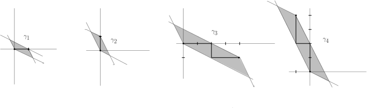
Figure 2. Irreducible animals $\Gamma_{1},\Gamma_{2},\Gamma_{3},\Gamma_{4}$; $\Gamma_{i}=[\gamma_{i},\emptyset]$.

Define

$$\Delta^{a}_{\epsilon}(\beta)=4a_{\epsilon}+(\beta-b_{\epsilon})\ {\rm and}\ \Delta^{b}_{\epsilon}(\beta)=4b_{\epsilon}+(\beta-a_{\epsilon})$$ (7.7)

By (7.1), both $\Delta^{a}_{\epsilon},\Delta^{b}_{\epsilon}\geq 0$. For $i=3,4$, the probabilities of $\Gamma_{i}=[\gamma_{i},\emptyset]$ are given by

$$\mathbb{P}_{\beta}^{\mathsf{h}_{\mathsf{x}}}(\Gamma_{3})={\rm e}^{-\beta-\Delta^{a}_{\epsilon}(\beta)}\ {\rm and}\ \mathbb{P}_{\beta}^{\mathsf{h}_{\mathsf{x}}}(\Gamma_{4})={\rm e}^{-\beta-\Delta^{b}_{\epsilon}(\beta)}.$$ (7.8)

We conclude:

$${\rm e}^{-a_{\epsilon}}+{\rm e}^{-b_{\epsilon}}+{\rm e}^{-\beta-\Delta^{a}_{\epsilon}(\beta)}+{\rm e}^{-\beta-\Delta^{b}_{\epsilon}(\beta)}=1-{\mathrm{O}}\left({\rm e}^{-2\beta}\right)$$ (7.9)

and

$$\begin{split}&\left({\rm e}^{-a_{\epsilon}}+4{\rm e}^{-\beta-\Delta^{a}_{\epsilon}(\beta)}-{\rm e}^{-\beta-\Delta^{b}_{\epsilon}(\beta)},{\rm e}^{-b_{\epsilon}}+4{\rm e}^{-\beta-\Delta^{b}_{\epsilon}(\beta)}-{\rm e}^{-\beta-\Delta^{a}_{\epsilon}(\beta)}\right)\\ &\quad=\mathbb{E}_{\beta}^{\mathsf{h}_{\mathsf{x}}}\mathsf{X}(\Gamma)+{\mathrm{O}}\left({\rm e}^{-2\beta}\right)\stackrel{{\scriptstyle\Delta}}{{=}}\mathsf{v}^{*}_{\epsilon}(\beta)+{\mathrm{O}}\left({\rm e}^{-2\beta}\right).\end{split}$$ (7.10)

Recall that $\mathsf{v}^{*}_{\epsilon}=\left|\mathsf{v}^{*}_{\epsilon}\right|_{1}(1-\epsilon,\epsilon)$. By (7.9) and (7.10), $\left|\mathsf{v}^{*}_{\epsilon}\right|_{1}\geq 1$.

From now on let us consider $\arg\left((1-\epsilon,\epsilon)\right)\in[0,\frac{2\pi}{5}]$. In this case the inspection of the first coordinate of the vector (7.10) (for the horizontal component) readily implies that $a_{\epsilon}\leq c_{5}$ uniformly in $\beta$ large. and, setting $\Delta_{\epsilon}=\Delta_{\epsilon}^{a}(\beta)=4a_{\epsilon}+(\beta-b_{\epsilon})$ (see (7.7)), we conclude: Uniformly in $\arg\left((1-\epsilon,\epsilon)\right)\in[0,\frac{2\pi}{5}]$. and $\beta$ large,

$$\begin{split}&{\rm e}^{-a_{\epsilon}}+{\rm e}^{-b_{\epsilon}}+{\rm e}^{-\beta-\Delta_{\epsilon}}=1-{\mathrm{O}}\left({\rm e}^{-2\beta}\right)\\ &\qquad\text{and}\\ &\left({\rm e}^{-a_{\epsilon}}+4{\rm e}^{-\beta-\Delta_{\epsilon}},{\rm e}^{-b_{\epsilon}}-{\rm e}^{-\beta-\Delta_{\epsilon}}\right)=\left|\mathsf{v}^{*}_{\epsilon}\right|_{1}\left(1-\epsilon,\epsilon\right)+{\mathrm{O}}\left({\rm e}^{-2\beta}\right).\end{split}$$ (7.11)

Proof of (7.4)

By (7.1), $b_{\epsilon}\leq\beta$, the first of (7.11) implies that $a_{\epsilon}\geq c_{6}{\rm e}^{-\beta}$ for any $\epsilon$ in question. Next, since by both of (7.11),

$$\left|\mathsf{v}^{*}_{\epsilon}\right|_{1}=1+{\mathrm{O}}\left({\rm e}^{-\beta-\Delta_{\epsilon}}\right),$$ (7.12)

the second of (7.11) (for the horizontal coordinate) implies that $a_{\epsilon}\stackrel{{\scriptstyle\sim}}{{=}}\epsilon$, uniformly in $\epsilon\geq c_{7}{\rm e}^{-\beta}$. Since $a_{\epsilon}$ is monotone non-decreasing in $\epsilon$, this implies that $a_{\epsilon}\leq c_{8}{\rm e}^{-\beta}$ for all $\epsilon\leq c_{7}{\rm e}^{-\beta}$, and the first claim (7.4) of Proposition 16 follows.

Proof of (7.5) and (7.6)

Consider now the second of (7.11) (for the vertical coordinate). In view of (7.12), and after multiplying both sides by ${\rm e}^{\beta}$, it reads (recall that $\Delta_{\epsilon}=4a_{\epsilon}+(\beta-b_{\epsilon})>\beta-b_{\epsilon}$):

$${\rm e}^{(\beta-b_{\epsilon})}-{\rm e}^{-(\beta-b_{\epsilon})}\leq{\rm e}^{(\beta-b_{\epsilon})}-{\rm e}^{-\Delta_{\epsilon}}=\epsilon{\rm e}^{\beta}+{\mathrm{O}}\left(\epsilon{\rm e}^{-\Delta_{\epsilon}}+{\rm e}^{-\beta}\right)\leq{\rm e}^{(\beta-b_{\epsilon})}.$$ (7.13)

If $\epsilon{\rm e}^{\beta}\geq 2$, then ${\mathrm{O}}\left(\epsilon{\rm e}^{-\Delta_{\epsilon}}+{\rm e}^{-\beta}\right)/(\epsilon{\rm e}^{\beta})={\mathrm{O}}\left({\frac{1}{\epsilon{\rm e}^{2\beta}}}\right)$. Hence, the first of (7.5).
Furthermore, since $\beta-b_{\epsilon}$ is non-increasing and non-negative, and since $a_{\epsilon}$ is non-negative and uniformly bounded,

$${\rm e}^{\beta-b_{\epsilon}}-{\rm e}^{-\Delta_{\epsilon}}={\rm e}^{\beta-b_{\epsilon}}-{\rm e}^{-(\beta-b_{\epsilon})-4a_{\epsilon}}\stackrel{{\scriptstyle\sim}}{{=}}(\beta-b_{\epsilon})+a_{\epsilon},$$

uniformly in $\epsilon\in[0,2{\rm e}^{-\beta}]$ and $\beta$ large. Hence, by (7.13),

$$(\beta-b_{\epsilon})+a_{\epsilon}\stackrel{{\scriptstyle\sim}}{{=}}\epsilon{\rm e}^{\beta}+{\mathrm{O}}\left(\epsilon{\rm e}^{-\Delta_{\epsilon}}+{\rm e}^{-\beta}\right),$$ (7.14)

also uniformly in $\epsilon\in[0,2{\rm e}^{-\beta}]$ and $\beta$ large. The asymptotic behavior of $a_{\epsilon}$ is already verified (7.4). Both the second of (7.5) and the upper bound (7.6) follow. ∎

Remark 17.

Consider $\mathsf{x}=\left|\mathsf{x}\right|_{1}\left(1-\epsilon,\epsilon\right)$, Since $\tau_{\beta}(\mathsf{x})=\mathsf{h}_{\mathsf{x}}\cdot\mathsf{x}=\beta\left|\mathsf{x}\right|_{1}-\left(a_{\mathsf{x}},b_{\mathsf{x}}\right)\cdot\mathsf{x}$, the asymptotics of surface tension $\tau_{\beta}$ are given by:

$$0\leq\left|\mathsf{x}\right|_{1}-\frac{\tau_{\beta}(\mathsf{x})}{\beta}={\left|\mathsf{x}\right|_{1}}\frac{(1-\epsilon)a_{\epsilon}+\epsilon b_{\epsilon}}{\beta},$$ (7.15)

where $a_{\epsilon}$ and $b_{\epsilon}$ comply with asymptotic relations (7.4), (7.5) and (7.6) uniformly in $\beta$ large and $\mathsf{x}\in\mathcal{Q}_{+}\cap\left\{{{\rm arg}(\mathsf{x})\in[0,2\pi/5]}\right\}$. In particular, the rescaled Wulff shape $(1/\beta){\mathbf{K}}_{\beta}$ tends to the square $Q=[-1,+1]^{2}$ in Hausdorff distance, as $\beta\to\infty$, and the boundary of $(1/\beta){\mathbf{K}}_{\beta}$ is at Hausdorff distance ${\mathrm{O}}\left(\frac{1}{\beta}\right)$ from $\partial Q$. Sharper asymptotics could be read from Proposition 16, in particular the boundary of $(1/\beta){\mathbf{K}}_{\beta}$ is within distance ${\mathrm{O}}\left(\frac{{\rm e}^{-\beta}}{\beta}\right)$ from $\partial Q$ along axis directions.

7.2. Decomposition of $\mathsf{R}_{k}$ and proof of Proposition 15.

The effective random walk $\mathsf{R}_{k}$ was defined in (5.1). We summarize computations of Subsection 7.1 as follows:

Definition 18.

Define the set of basic steps as $\mathfrak{S}_{0}=\left\{\mathsf{e}_{1},\mathsf{e}_{2},4\mathsf{e}_{1}-\mathsf{e}_{2}\right\}$.

The probabilities of three basic steps are given by

$$\mathbb{P}_{\beta}^{\mathsf{h}_{\mathsf{x}}}\left(\mathsf{X}=\mathsf{e}_{1}\right)={\rm e}^{-a_{\mathsf{x}}(\beta)},\ \mathbb{P}_{\beta}^{\mathsf{h}_{\mathsf{x}}}\left(\mathsf{X}=\mathsf{e}_{2}\right)={\rm e}^{-b_{\mathsf{x}}(\beta)}\ {\rm and}\ \mathbb{P}_{\beta}^{\mathsf{h}_{\mathsf{x}}}\left(\mathsf{X}=4\mathsf{e}_{1}-\mathsf{e}_{2}\right)={\rm e}^{-\beta-\Delta_{\mathsf{x}}(\beta)}.$$ (7.16)

The coefficients $a_{\mathsf{x}},b_{\mathsf{x}}$ and $\Delta_{\mathsf{x}}=4a_{\mathsf{x}}+(\beta-b_{\mathsf{x}})$ satisfy asymptotic relations (7.4), (7.5) and (7.6).
Non-basic steps do not contribute in the following sense:

$$\sup_{{\rm arg}(\mathsf{x})\in[0,2\pi/5]}\sum_{\mathsf{y}\not\in\mathfrak{S}_{0}}\left|\mathsf{y}\right|^{2}\mathbb{P}_{\beta}^{\mathsf{h}_{\mathsf{x}}}\left(\mathsf{X}=\mathsf{y}\right)={\mathrm{O}}\left({\rm e}^{-2\beta}\right).$$ (7.17)

Remark 19.

Note that for fixed $\epsilon>0$ and for any $\mathsf{x}$ with $\frac{\mathsf{x}}{\left|\mathsf{x}\right|_{1}}=(1-\epsilon,\epsilon)$ the probability $\mathbb{P}_{\beta}^{\mathsf{h}_{\mathsf{x}}}(\mathsf{X}=4\mathsf{e}_{1}-\mathsf{e}_{2})$ is (asymptotically in $\beta$) of order ${\rm e}^{-2\beta}$. However, for $\epsilon$-s of order ${\rm e}^{-\beta}$ the probability of $\mathbb{P}_{\beta}^{\mathsf{h}_{\mathsf{x}}}(\mathsf{X}=4\mathsf{e}_{1}-\mathsf{e}_{2})$ is comparable to $\mathbb{P}_{\beta}^{\mathsf{h}_{\mathsf{x}}}(\mathsf{X}=\mathsf{e}_{2})$. For the sake of a unified exposition we always include $4\mathsf{e}_{1}-\mathsf{e}_{2}$ to the set of basic steps $\mathfrak{S}_{0}$.

Recall our notation $\mathsf{v}^{*}(\beta,\mathsf{x})=\mathsf{v}^{*}(\beta,\mathsf{h}_{\mathsf{x}})=\mathbb{E}_{\beta}^{\mathsf{h}_{\mathsf{x}}}\left(\mathsf{X}(\Gamma)\right)$ for the mean displacement over an irreducible animal sampled from $\left(\mathsf{A},\mathbb{P}_{\beta}^{\mathsf{h}_{\mathsf{x}}}\right)$. By (7.10) and (7.17),

$$\mathsf{v}^{*}(\beta,\mathsf{x})=\left({\rm e}^{-a_{\mathsf{x}}(\beta)},{\rm e}^{-b_{\mathsf{x}}(\beta)}\right)+{\rm e}^{-\beta-\Delta_{\mathsf{x}}(\beta)}\left(4,-1\right)+{\mathrm{O}}\left({\rm e}^{-2\beta}\right).$$ (7.18)

By Theorem 4, $\mathsf{v}^{*}(\beta,\mathsf{x})$ points in the direction of $\mathsf{x}$, in other words there exists $\ell_{\mathsf{x}}\in\mathbb{R}_{+}$ such that

$$\mathsf{x}=\ell_{\mathsf{x}}\mathsf{v}^{*}(\beta,\mathsf{x}),$$ (7.19)

writing $\mathsf{x}=\left|\mathsf{x}\right|_{1}\left(1-\epsilon,\epsilon\right)$, we, in view of the first of (7.11), conclude that

$$\ell_{\mathsf{x}}=\left|\mathsf{x}\right|_{1}\left(1+{\mathrm{O}}\left({\rm e}^{-\left(\beta+\Delta_{\mathsf{x}}(\beta)\right)}\right)\right),$$ (7.20)

and, as a consequence, that

$${\left|\left({\rm e}^{-a_{\mathsf{x}}(\beta)}+4{\rm e}^{-\beta-\Delta_{\mathsf{x}}(\beta)},{\rm e}^{-b_{\mathsf{x}}(\beta)}-{\rm e}^{-\beta-\Delta_{\mathsf{x}}(\beta)}\right)-(1-\epsilon,\epsilon)\right|_{{1}}\leq c{\rm e}^{-\beta-\Delta_{\mathsf{x}}(\beta)},}$$ (7.21)

uniformly in ${\rm arg}(\mathsf{x})\in[0,\frac{2\pi}{5}]$ and $\beta$ large.

Decomposition of $\mathsf{R}_{k}$.

We shall always represent random walk $\mathsf{R}_{k}$ as

$$\mathsf{R}_{k}=\sum_{1}^{k}\left(\xi_{i}\mathsf{U}_{i}+(1-\xi_{i})\mathsf{V}_{i}\right),$$ (7.22)

where

1. $\left\{\xi_{i}\right\}$ is a sequence of i.i.d. Bernoulli random variables with probability of success $\mathbb{P}(\xi_{i}=1)=q$;

   $$q=\alpha_{\mathsf{x}}^{1}{\rm e}^{-a_{\mathsf{x}}(\beta)}+\alpha_{\mathsf{x}}^{2}{\rm e}^{-b_{\mathsf{x}}(\beta)}.$$ (7.23)

   There are two different choices of $\alpha_{\mathsf{x}}^{i}\in[0,1]$, according to the direction $\mathsf{x}$, as described in CASE 1 and CASE 2 below. In both cases, however, $q$ in (7.23) will satisfy:

   $${1-q\stackrel{{\scriptstyle\sim}}{{=}}{\rm e}^{-(\beta+\Delta_{\mathsf{x}})}.}$$ (7.24)

2. $\left\{\mathsf{U}_{i}\right\}$ is an independent (from $\left\{\xi_{i}\right\}$) sequence of i.i.d random vectors which take values $(1,0)$ and $(0,1)$ with probabilities

   $$1-p=\mathbb{P}\left(\mathsf{U}_{i}=(1,0)\right)=\frac{{\alpha_{\mathsf{x}}^{1}}{\rm e}^{-a_{\mathsf{x}}(\beta)}}{\alpha_{\mathsf{x}}^{1}{\rm e}^{-a_{\mathsf{x}}(\beta)}+\alpha_{\mathsf{x}}^{2}{\rm e}^{-b_{\mathsf{x}}(\beta)}},$$ (7.25)

   and $\mathbb{P}\left(\mathsf{U}_{i}=(0,1)\right)=p$, respectively.

3. $\left\{\mathsf{V}_{i}\right\}$ is yet another independent (from $\left\{\xi_{i}\right\}$ and $\left\{\mathsf{U}_{i}\right\}$) sequence of i.i.d. random vectors with

   $$\begin{split}&\mathbb{P}\left(\mathsf{V}_{i}=\mathsf{e}_{1}\right)=\frac{(1-\alpha_{\mathsf{x}}^{1}){\rm e}^{-a_{\mathsf{x}}}}{1-q},\quad\mathbb{P}\left(\mathsf{V}_{i}=\mathsf{e}_{2}\right)=\frac{(1-\alpha_{\mathsf{x}}^{2}){\rm e}^{-b_{\mathsf{x}}}}{1-q}\\ &\qquad\text{and, for $\mathsf{y}\neq\mathsf{e}_{1},\mathsf{e}_{2}$,}\ \mathbb{P}\left(\mathsf{V}_{i}=\mathsf{y}\right)=\frac{1}{1-q}\mathbb{P}_{\beta}^{\mathsf{h}}(\mathsf{X}(\Gamma)=\mathsf{y}).\end{split}$$ (7.26)

By (4.11) for any choice of $\alpha_{\mathsf{x}}^{i}\in[0,1]$ as above the distribution of $\mathsf{V}_{i}$ has exponential tails: $\exists r_{0},\nu_{0}>0\ \text{such that}$

$$\mathbb{P}\left(\left|\mathsf{V}_{i}\right|>r\right){\leq}{\rm e}^{-\beta\nu_{0}r}\ \text{uniformly in $r\geq r_{0}$, $\mathsf{x}$ and $\beta$ large}.$$ (7.27)

In addition, we shall choose $\alpha_{\mathsf{x}}^{i}\in[0,1]$ in such a way that the distribution of $\mathsf{V}_{i}$ will be uniformly non-degenerate in the following sense: There exist $\delta_{1},\delta_{2}\in(0,1)$ such that

$$\delta_{1}\leq\min{\left\{\mathbb{P}\left(\mathsf{V}_{i}=\mathsf{e}_{2}\right),\mathbb{P}\left(\mathsf{V}_{i}=4\mathsf{e}_{1}-\mathsf{e}_{2}\right)\right\}}\ {\rm and}\ \mathbb{E}\mathsf{V}\cdot\mathsf{e}_{1}\in[\delta_{2},\delta_{2}^{-1}].$$ (7.28)

uniformly in ${\rm arg}(\mathsf{x})\in[0,\frac{2\pi}{5}]$ and $\beta$ large.

Let $N_{\ell}$ be the number of failures (zeros) of $\left\{\xi_{i}\right\}$ until the $\ell$-th success, and let $\mathsf{R}^{\mathsf{U}}$ and $\mathsf{R}^{\mathsf{V}}$ be the random walks with steps $\left\{\mathsf{U}_{i}\right\}$ and $\left\{\mathsf{V}_{i}\right\}$. Then,

$$\begin{split}&\sum_{\ell,m}\mathbb{P}(N_{\ell}=m)\sum_{\mathsf{y}}\mathbb{P}(\mathsf{R}_{\ell}^{U}=\mathsf{y})\mathbb{P}(\mathsf{R}^{V}_{m}=\mathsf{x}-\mathsf{y})\\ &\quad\leq\mathbb{P}_{\beta}^{\mathsf{h}}\left(0,\mathsf{x}\right){\leq c_{2}\sum_{\ell,m}\mathbb{P}(N_{\ell}=m)\sum_{\mathsf{y}}\mathbb{P}(\mathsf{R}_{\ell}^{U}=\mathsf{y})\mathbb{P}(\mathsf{R}^{V}_{m}=\mathsf{x}-\mathsf{y}).}\end{split}$$ (7.29)

Indeed, the difference between $\mathbb{P}_{\beta}^{\mathsf{h}}\left(0,\mathsf{x}\right)$ and the l.h.s. sum in (7.29) is that the former takes into account all possible superpositions of steps of $\mathsf{U}$ and $\mathsf{V}$ walks, whereas the latter ignores the situation when $\mathsf{x}$ is hit by a $\mathsf{V}$-step. The upper bound in (7.29) follows from (7.24).

Proof of Proposition 15.

We now turn to an analysis of (7.29). It would be helpful to remember that by (7.19) the running scale $\ell_{\mathsf{x}}$ satisfies:

$$q\ell_{\mathsf{x}}\left(1-p,p\right)+(1-q)\ell_{\mathsf{x}}\mathbb{E}V_{i}\stackrel{{\scriptstyle\Delta}}{{=}}\ell_{\mathsf{x}}^{{\mathsf{u}}}(1-p,p)+\ell_{\mathsf{x}}^{{\mathsf{v}}}\mathbb{E}\mathsf{V}_{i}=\mathsf{x},$$ (7.30)

where we have defined $\ell_{\mathsf{x}}^{{\mathsf{u}}}=q\ell_{\mathsf{x}}$ and $\ell_{\mathsf{x}}^{{\mathsf{v}}}=(1-q)\ell_{\mathsf{x}}$. We shall rely on the elementary Lemma 20 below, which is claimed to hold uniformly in i.i.d sequences $\left\{\mathsf{V}_{i}\right\}$ satisfying (7.27) and (7.28): Let us fix $C\in(0,\infty)$ and, given $\mathsf{u}\in\mathbb{R}^{2}$ and $r\in\mathbb{N}$ define

$$\Lambda_{r}(\mathsf{u})=\mathsf{u}+\{[-Cr,\dots,Cr]\times[-r,r]\}.$$

For a horizontal lattice line $\mathcal{B}$ let us say that $\mathcal{B}\cap\Lambda_{r}(\mathsf{u})\neq\emptyset$ if $\mathcal{B}$ passes through $\Lambda_{r}(\mathsf{u})$.

Lemma 20.

There exist $C=C(\delta,r_{0},\nu_{0})$ and $c=c(\delta,r_{0},\nu_{0})$ such that

$$\sum_{\left|k-{n}\right|\leq cr}\mathbb{P}\left(\mathsf{R}^{\mathsf{V}}_{k}\in\mathcal{B}\cap\Lambda_{r}({n}\mathbb{E}\mathsf{V})\right)\stackrel{{\scriptstyle\sim}}{{=}}\frac{r^{2}}{{n}\vee 1}$$ (7.31)

uniformly in ${n\geq 0}$, integers $r\leq\sqrt{{n}}\vee 1$, horizontal lines ${\mathcal{B}\cap\Lambda_{r}(n\mathbb{E}\mathsf{V})\neq\emptyset}$ and $\beta$ large.

Sketch of the proof:

Eq. (7.31) is a coarse estimate, and the logic behind it should be transparent: By (7.27) $\mathsf{V}_{i}$-s have exponential tails. On the other hand, (7.28) yields a lower bound on the non-degeneracy of covariance structure of $\mathsf{V}_{i}$. A usual local limit analysis implies that one can choose $c$ and $C$ in such a way that $\mathbb{P}\left(\mathsf{R}^{\mathsf{V}}_{k}\in\mathcal{B}\cap\Lambda_{r}(n\mathbb{E}\mathsf{V})\right)\stackrel{{\scriptstyle\sim}}{{=}}\frac{r}{n\vee 1}$ uniformly in all lines $\mathcal{B}\cap\Lambda_{r}(n\mathbb{E}\mathsf{V})\neq\emptyset$ and in all times $k$ with $\left|k-n\right|\leq cr$.

Let us fix a sufficiently large constant $c_{0}$. How exactly it is fixed is explained below when we consider CASE 2.

CASE 1. $\epsilon\leq c_{0}{\rm e}^{-\beta}$. By Proposition 16 in this regime the probabilities $\mathbb{P}_{\beta}^{\mathsf{x}}(\Gamma_{2})={\rm e}^{-b_{\epsilon}}$ and $\mathbb{P}_{\beta}^{\mathsf{x}}(\Gamma_{3})={\rm e}^{-\beta-\Delta_{\epsilon}}$ are of the same order ${\rm e}^{-\beta}$. Consequently, if we take $\alpha^{2}_{\mathsf{x}}=p=0$ and $\alpha_{\mathsf{x}}^{1}=1$, both (7.24) and, also in view of (7.17), (7.28) are satisfied.

If $p=0$, then the $\mathsf{R}^{U}$-walk is trivial: $\mathbb{P}\left(\mathsf{R}^{U}_{k}=(\ell,0)\right)=\delta_{k\ell}$. Consequently, (7.29) takes a particular simple form:

$$\mathbb{P}_{\beta}^{\mathsf{h}}\left(0,\mathsf{x}\right)\stackrel{{\scriptstyle\sim}}{{=}}\sum_{\ell,m}\mathbb{P}(N_{\ell}=m)\mathbb{P}\left(\mathsf{R}^{\mathsf{V}}_{m}=(x_{1}-\ell,x_{2})\right).$$ (7.32)

Recall how $\ell_{\mathsf{x}}^{{\mathsf{u}}}$ and $\ell_{\mathsf{x}}^{{\mathsf{v}}}$ were defined in (7.30). Note that $\ell_{\mathsf{x}}^{{\mathsf{u}}}=\frac{q}{1-q}\ell_{\mathsf{x}}^{{\mathsf{v}}}$. By construction $p=0$. Consequently, $(x_{1}-\ell,x_{2})=\mathsf{x}-(\ell,0)=(\ell_{\mathsf{x}}^{{\mathsf{u}}}-\ell,0)+\ell_{\mathsf{x}}^{{\mathsf{v}}}\mathbb{E}\mathsf{V}$, and

$$\mathbb{P}\left(\mathsf{R}^{\mathsf{V}}_{m}=(x_{1}-\ell,x_{2})\right)=\mathbb{P}\left(\mathsf{R}^{\mathsf{V}}_{m}=\mathbb{E}\mathsf{R}^{\mathsf{V}}_{m}-(m-\ell_{\mathsf{x}}^{{\mathsf{v}}})\mathbb{E}\mathsf{V}-(\ell-\ell_{\mathsf{x}}^{{\mathsf{u}}},0)\right).$$

In view of the last of (7.28), the main contribution to (7.32) should come from the values of $m$ and $\ell$ satisfying

$$\left|m-\ell_{\mathsf{x}}^{{\mathsf{v}}}\right|\leq c_{3}\sqrt{\ell_{\mathsf{x}}^{{\mathsf{v}}}}\ {\rm and}\ \left|\ell-\ell_{\mathsf{x}}^{{\mathsf{u}}}\right|\leq c_{3}\sqrt{\ell_{\mathsf{x}}^{{\mathsf{v}}}}.$$

Let us estimate (7.32) for the values of $m$ and $\ell$ restricted to the latter region. By a direct application of Stirling formula,

$$\mathbb{P}(N_{\ell}=m)\stackrel{{\scriptstyle\sim}}{{=}}\frac{1}{\sqrt{\ell_{\mathsf{x}}^{{\mathsf{v}}}}\vee 1}$$ (7.33)

uniformly in $\left|m-\ell_{\mathsf{x}}^{{\mathsf{v}}}\right|\leq c_{3}\sqrt{\ell_{\mathsf{x}}^{{\mathsf{v}}}}$ and $\left|\ell-\ell_{\mathsf{x}}^{{\mathsf{u}}}\right|\leq c_{3}\sqrt{\ell_{\mathsf{x}}^{{\mathsf{v}}}}$. Furthermore, there exists $c<\infty$, such that

$$\mathbb{P}(N_{\ell}=m)\leq\frac{c}{\sqrt{\ell_{\mathsf{x}}^{{\mathsf{v}}}}\vee 1}$$ (7.34)

for every $m$.

An application of Lemma 20 with $r=\sqrt{\ell_{\mathsf{x}}^{{\mathsf{v}}}}\vee 1$ implies, therefore:

$$\sum_{\left|\ell^{\prime}\right|\leq c_{3}\sqrt{\ell_{\mathsf{x}}^{{\mathsf{v}}}}}\ \sum_{\left|m-\ell_{\mathsf{x}}^{{\mathsf{v}}}\right|\leq c_{3}\sqrt{\ell_{\mathsf{x}}^{{\mathsf{v}}}}}\mathbb{P}\left(\mathsf{R}^{\mathsf{V}}_{m}=\mathbb{E}\mathsf{R}^{\mathsf{V}}_{\ell_{\mathsf{x}}^{{\mathsf{v}}}}+\left(\ell^{\prime},0\right)\right)\stackrel{{\scriptstyle\sim}}{{=}}1.$$ (7.35)

Together with (7.33) and (7.34) this implies that

$$\mathbb{P}_{\beta}^{\mathsf{h}}\left(0,\mathsf{x}\right)\stackrel{{\scriptstyle\sim}}{{=}}\frac{1}{\sqrt{\ell_{\mathsf{x}}^{{\mathsf{v}}}}\vee 1}{\stackrel{{\scriptstyle\sim}}{{=}}\frac{1}{\sqrt{{\rm e}^{-b_{\mathsf{x}}(\beta)}\left|\mathsf{x}\right|_{1}}\vee 1},}$$ (7.36)

uniformly in $\beta$ large and $\mathsf{x}$-s complying with CASE 1. The last asymptotic equivalence; $\ell_{\mathsf{x}}^{{\mathsf{v}}}\stackrel{{\scriptstyle\sim}}{{=}}{\rm e}^{-b_{\mathsf{x}}(\beta)}\left|\mathsf{x}\right|_{1}$, holds since by (7.30), (7.20) and by (7.24),

$$\ell_{\mathsf{x}}^{{\mathsf{v}}}=(1-q)\ell_{\mathsf{x}}\stackrel{{\scriptstyle\sim}}{{=}}(1-q)\left|\mathsf{x}\right|_{1}\stackrel{{\scriptstyle\sim}}{{=}}{\rm e}^{-\beta-\Delta_{\mathsf{x}}}\left|\mathsf{x}\right|_{1}.$$

However, by Proposition 16, ${\rm e}^{-\beta-\Delta_{\mathsf{x}}}\stackrel{{\scriptstyle\sim}}{{=}}{\rm e}^{-\beta}\stackrel{{\scriptstyle\sim}}{{=}}{\rm e}^{-b_{\mathsf{x}}}$ uniformly in $\epsilon\leq c_{0}{\rm e}^{-\beta}$ and $\beta$ large.

CASE 2. $\epsilon>c_{0}{\rm e}^{-\beta}$. By (7.17) there exists $\eta>0$ such that

$${\rm e}^{-\beta-\Delta_{\epsilon}}\geq\eta\sum_{\mathsf{y}\neq\mathsf{e}_{1},\mathsf{e}_{2}}\left|\mathsf{y}\right|_{1}\mathbb{P}_{\beta}^{\mathsf{h}_{\epsilon}}\left(\mathsf{X}=\mathsf{y}\right),$$ (7.37)

uniformly in $\beta$ large and $\arg\left((1-\epsilon,\epsilon)\right)\in[0,\frac{2\pi}{5}]$. We shall choose $\alpha_{\epsilon}^{i}$ in the decomposition (7.22) of $R_{k}$ as follows

$$\left(1-\alpha_{\epsilon}^{1}\right){\rm e}^{-a_{\epsilon}}=\frac{1}{\eta}{\rm e}^{-\beta-\Delta_{\epsilon}}\ {\rm and}\ \left(1-\alpha_{\epsilon}^{2}\right){\rm e}^{-b_{\epsilon}}={\rm e}^{-\beta-\Delta_{\epsilon}}.$$ (7.38)

Since $a_{\epsilon}$ is uniformly bounded and $b_{\epsilon}<\beta<\beta+\Delta_{\epsilon}$, (7.38) is a feasible choice. In view of (7.37) we readily verify (7.28) and also (7.24). In fact recalling how $q$ was defined in (7.23), we, in view of (7.37), infer that under (7.38) $1-q$ satisfies the following bound

$$1-q\in{\rm e}^{-\beta-\Delta_{\epsilon}}\left(2+\frac{1}{\eta},2+\frac{2}{\eta}\right),$$ (7.39)

uniformly in $\beta$ large and $\epsilon>c_{0}{\rm e}^{-\beta}$. Furthermore, by (7.5) there exists $c_{4}<\infty$ such that

$$b_{\epsilon}\leq\beta-\log c_{0}+c_{4}{\rm e}^{-\beta}\ {\rm and}\ \Delta_{\epsilon}\geq\log c_{0}-c_{4}{\rm e}^{-\beta},$$ (7.40)

uniformly in $c_{0}\geq 2$, $\beta$ large and $\epsilon>c_{0}{\rm e}^{-\beta}$. This means (see (7.30) for the definition of $\ell_{\mathsf{x}}^{{\mathsf{u}}}$ and $\ell_{\mathsf{x}}^{{\mathsf{v}}}$) that

$$\ell_{\mathsf{x}}^{{\mathsf{v}}}=\frac{1-q}{q}\ell_{\mathsf{x}}^{{\mathsf{u}}}\leq p\ell_{\mathsf{x}}^{{\mathsf{u}}}\stackrel{{\scriptstyle\sim}}{{=}}x_{2}\stackrel{{\scriptstyle\sim}}{{=}}\left|\mathsf{x}\right|_{1}{\rm e}^{-b_{\mathsf{x}}},$$ (7.41)

also uniformly in CASE 2. Indeed, the last equivalence follows from (7.21) and Proposition 16 choosing $c_{0}$ large. On the other hand, going back to the definition of $p$ in (7.25), the choice of $\alpha_{\epsilon}^{2}$ in in (7.38) implies that $p\geq{\rm e}^{-b_{\epsilon}}-{\rm e}^{-\beta-\Delta_{\epsilon}}$. Comparing with (7.39), and in view of (7.40), we conclude that $p\geq(1-q)/q$ as soon as $c_{0}$ is large enough. Hence the first inequality in (7.41).

Let us go back to (7.29) and write:

$$\mathbb{P}_{\beta}^{\mathsf{h}}\left(0,\mathsf{x}\right)\stackrel{{\scriptstyle\sim}}{{=}}\sum_{\ell,m}\mathbb{P}(N_{\ell}=m)\sum_{r}\mathbb{P}(\mathsf{R}_{\ell}^{\mathsf{U}}=(\ell-r,r)\mathbb{P}\left(\mathsf{R}^{\mathsf{V}}_{m}=\mathsf{x}-(\ell-r,r)\right)$$ (7.42)

By Stirling’s formula the main contribution to

$$\mathbb{P}(N_{\ell}=m)\stackrel{{\scriptstyle\sim}}{{=}}\frac{1}{\sqrt{m}}\ \text{ comes from $\left|\ell-\frac{q}{1-q}m\right|\leq c_{4}\sqrt{m}$}.$$ (7.43)

Next, since $\mathbb{E}\mathsf{R}_{\ell}^{\mathsf{U}}=\ell(1-p,p)$,

$$\mathbb{P}\left(\mathsf{R}_{\ell}^{\mathsf{U}}=(\ell-n,n)\right)=\mathbb{P}\left(\mathsf{R}_{\ell}^{\mathsf{U}}=\mathbb{E}\mathsf{R}_{\ell}^{\mathsf{U}}+(\ell p-n,n-\ell p)\right),$$

and consequently, again by Stirling’s formula, the main contribution to

$$\mathbb{P}\left(\mathsf{R}_{\ell}^{\mathsf{U}}=(\ell-n,n)\right)\stackrel{{\scriptstyle\sim}}{{=}}\frac{1}{\sqrt{p\ell}}\ \text{comes from $\left|n-\ell p\right|\leq c_{5}\sqrt{\ell p}$}.$$ (7.44)

Recall (7.30) that $\mathsf{x}=\ell_{\mathsf{x}}^{{\mathsf{u}}}(1-p,p)+\ell_{\mathsf{x}}^{{\mathsf{v}}}\mathbb{E}\mathsf{V}$. Therefore, setting $\bar{n}=p\ell_{\mathsf{x}}^{{\mathsf{u}}}$,

$$\begin{split}\mathsf{x}-(\ell-n,n)&=\mathbb{E}\mathsf{R}_{\ell_{\mathsf{x}}^{{\mathsf{v}}}}^{\mathsf{V}}+\left((\ell_{\mathsf{x}}^{{\mathsf{u}}}-\ell)-(\bar{n}-n),(\bar{n}-n)\right)\\ &=\mathbb{E}\mathsf{R}_{m}^{\mathsf{V}}+(\ell_{\mathsf{x}}^{{\mathsf{v}}}-m)\mathbb{E}\mathsf{V}+\left((\ell_{\mathsf{x}}^{{\mathsf{u}}}-\ell)-(\bar{n}-n),(\bar{n}-n)\right).\end{split}$$ (7.45)

Since we restrict attention to $\ell$ and $m$ satisfying the second of (7.43), and since $\ell_{\mathsf{x}}^{{\mathsf{u}}}=\frac{q}{1-q}\ell_{\mathsf{x}}^{{\mathsf{v}}}$, the main contribution to

$$\mathbb{P}\left(\mathsf{R}^{\mathsf{V}}_{m}=\mathsf{x}-(\ell-n,n)\right)\ \text{comes from $\left|m-\ell_{\mathsf{x}}^{{\mathsf{v}}}\right|,\left|\ell-\ell_{\mathsf{x}}^{{\mathsf{u}}}\right|,\left|n-\bar{n}\right|\leq c_{6}\sqrt{\ell_{\mathsf{x}}^{{\mathsf{v}}}}$}.$$ (7.46)

Let us go back to (7.42). In view of (7.43)-(7.46),

$$\mathbb{P}_{\beta}^{\mathsf{h}}\left(0,\mathsf{x}\right)\stackrel{{\scriptstyle\sim}}{{=}}\frac{1}{\sqrt{p\ell_{\mathsf{x}}^{{\mathsf{u}}}}}\frac{1}{\sqrt{\ell_{\mathsf{x}}^{{\mathsf{v}}}}\vee 1}{\sum}^{*}\mathbb{P}\left(\mathsf{R}^{\mathsf{V}}_{m}=\mathbb{E}\mathsf{R}_{\ell_{\mathsf{x}}^{{\mathsf{v}}}}^{\mathsf{V}}+\left((\ell_{\mathsf{x}}^{{\mathsf{u}}}-\ell)-(\bar{n}-n),(\bar{n}-n)\right)\right)$$ (7.47)

where

$${\sum}^{*}\stackrel{{\scriptstyle\Delta}}{{=}}\sum_{\left|\ell-\ell_{\mathsf{x}}^{{\mathsf{u}}}\right|\leq c_{7}\sqrt{\ell_{\mathsf{x}}^{{\mathsf{v}}}}\vee 1}\ \sum_{\left|n-\bar{n}\right|\leq c_{7}\sqrt{\ell_{\mathsf{x}}^{{\mathsf{v}}}}\vee 1}\ \sum_{\left|m-\ell_{\mathsf{x}}^{{\mathsf{v}}}\right|\leq c_{7}\sqrt{\ell_{\mathsf{x}}^{{\mathsf{v}}}}\vee 1}.$$

By an application of Lemma 20 (again with $r=\sqrt{\ell_{\mathsf{x}}^{{\mathsf{v}}}}\vee 1$), and in view of (7.41),

$$\mathbb{P}_{\beta}^{\mathsf{h}}\left(0,\mathsf{x}\right)\stackrel{{\scriptstyle\sim}}{{=}}\frac{1}{\sqrt{x_{2}}}{\stackrel{{\scriptstyle\sim}}{{=}}\frac{1}{\sqrt{{\rm e}^{-b_{\mathsf{x}}(\beta)}\left|\mathsf{x}\right|_{1}}}},$$ (7.48)

uniformly in CASE 2.

Putting (7.36) and (7.48) together we deduce the claim (7.3) of Proposition 15. ∎

7.3. Alili-Doney representation.

The (strict) event $\hat{\mathfrak{R}}_{\ell}^{+}$ is defined similarly to (5.3),

$${\hat{\mathfrak{R}}_{\ell}^{+,\mathsf{n}}(\mathsf{w},\mathsf{z})=\left\{\underline{\Gamma}:\,S_{1},\dots,S_{\ell-1}>0;\mathsf{R}_{0}=\mathsf{w},\mathsf{R}_{\ell}=\mathsf{z}\right\}.}$$ (7.49)

In order to explore $\mathbb{P}_{\beta,+}^{\mathsf{h}}(\mathsf{w},\mathsf{z})=\sum_{\ell}\mathbb{P}_{\beta}^{\mathsf{h}}\left(\mathfrak{R}_{\ell}^{+,\mathsf{n}}(\mathsf{w},\mathsf{z})\right)$-terms in (6.4) we need both strict and non-strict events . Indeed, define $\hat{\mathbb{P}}_{\beta,+}^{\mathsf{h}}(\mathsf{w},\mathsf{z})=\sum_{\ell}\mathbb{P}_{\beta}^{\mathsf{h}}\left(\hat{\mathfrak{R}}_{\ell}^{+,\mathsf{n}}(\mathsf{w},\mathsf{z})\right)$ Then, the decomposition of effective random walk trajectory $\left(\mathsf{w}=\mathsf{R}_{0},\dots,\mathsf{R}_{\ell}=\mathsf{z}\right)$ with respect to the first absolute minimum $\mathsf{y}=\mathsf{R}_{k}$;

$$\mathsf{y}\cdot\mathsf{n}=\min_{m}\mathsf{R}_{m}\cdot\mathsf{n}\quad{\rm and}\quad\mathsf{R}_{m}\cdot\mathsf{n}>\mathsf{y}\cdot\mathsf{n}\ \text{for any $m<k$},$$

yields:

$$\mathbb{P}_{\beta,+}^{\mathsf{h}}\left(\mathsf{w},\mathsf{z}\right)=\sum_{\mathsf{y}}\hat{\mathbb{P}}_{\beta,+}^{\mathsf{h}}\left(\mathsf{w}-\mathsf{y},0\right)\mathbb{P}_{\beta,+}^{\mathsf{h}}\left(0,\mathsf{z}-\mathsf{y}\right),$$ (7.50)

Non-strict ascending ladder height $H_{1}$ of $S_{\ell}$ is defined via

$$H_{1}=S_{\tau_{1}}\quad{\rm where}\quad\tau_{1}=\min\{\ell>0\,:\,S_{\ell}\geq S_{0}\}$$ (7.51)

$H_{2},H_{3},\dots$ are defined recursively.

Strict descending ladder height $\hat{H}_{1}$ of $S_{\ell}$ is defined via

$$\hat{H}_{1}=S_{\hat{\tau}_{1}}\quad{\rm where}\quad\hat{\tau}_{1}=\min\{\ell>0\,:\,S_{\ell}{<}S_{0}\}$$ (7.52)

$\hat{H}_{2},\hat{H}_{3},\dots$ are defined recursively.

Let $N^{+}_{m}(z)$ be the total number of non-negative non-strict ladder heights $H_{i}\leq z$ reached during first $m$ steps by the effective random walk $S_{\ell}$ defined in (5.2). Similarly. let $N^{-}_{m}(z)$ be the total number of non-negative strict descending ladder heights $\hat{H}_{j}\leq z$ reached during the first $m$ steps of $S_{\ell}$. We drop sub-index $m$ whenever talking about $m=\infty$ (that is whenever talking about the total number of ladder heights).

For $\mathsf{t}\in\mathcal{H}_{+,\mathsf{n}}$ define events

$$\mathcal{L}^{+}_{\mathsf{t}}=\left\{\exists\,i:\mathsf{R}_{\tau_{i}}=\mathsf{t}\right\}\quad\text{and}\quad\mathcal{L}^{-}_{\mathsf{t}}=\left\{\exists\,i:\mathsf{R}_{\hat{\tau}_{i}}=\mathsf{t}\right\}.$$ (7.53)

Then, recalling that $\mathfrak{A}_{m}(\mathsf{x},\mathsf{y})$ was defined just after (4.8),

$$\hat{\mathbb{P}}_{\beta,+}^{\mathsf{h}}\left(\mathsf{v},0\right)=\sum_{m}\mathbb{P}_{\beta}^{\mathsf{h}}\left(\mathfrak{A}_{m}(\mathsf{v},0);\mathcal{L}^{-}_{0}\right)\ {\rm and}\ \mathbb{P}_{\beta,+}^{\mathsf{h}}\left(0,\mathsf{v}\right)=\sum_{m}\mathbb{P}_{\beta}^{\mathsf{h}}\left(\mathfrak{A}_{m}(0,\mathsf{v});\mathcal{L}^{+}_{\mathsf{v}}\right).$$ (7.54)

The first of (7.54) is straightforward. The second follows by a well-known rearrangement argument: If $s=\sum_{1}^{m}s_{j}$ and $\sum_{1}^{k}s_{j}\geq 0$ for any $k$, then $\hat{S}_{k}=\sum_{m-k+1}^{m}s_{j}$ for $k=1...m$ satisfies $\hat{S}_{m}=s=\max_{k}\hat{S}_{k}$.

An adaptation of the combinatorial lemma by Alili and Doney [1] for the effective random walk setup was formulated [3]. In particular, for any $\mathsf{v}\in\mathcal{Q}_{+}\setminus 0$ and $\mathsf{n}$,

$$\begin{split}\mathbb{P}_{\beta,+}^{\mathsf{h}}\left(0,\mathsf{v}\right)&=\sum_{m}\frac{1}{m}\,\mathbb{E}_{\beta}^{\mathsf{h}}\left({\mathfrak{A}_{m}}(0,\mathsf{v})\,;\,N^{+}_{m}(\mathsf{v}\cdot\mathsf{n})\right){\stackrel{{\scriptstyle\sim}}{{=}}\frac{1}{\left|\mathsf{v}\right|_{1}}\sum_{\frac{\left|\mathsf{v}\right|_{1}}{c}\leq m\leq c\left|\mathsf{v}\right|_{1}}\!\!\!\!\!\!\!\mathbb{E}_{\beta}^{\mathsf{h}}\left({\mathfrak{A}_{m}}(0,\mathsf{v})\,;\,N^{+}_{m}(\mathsf{v}\cdot\mathsf{n})\right)}\\ &\quad{\rm and}\\ \hat{\mathbb{P}}_{\beta,+}^{\mathsf{h}}\left(\mathsf{v},0\right)&=\sum_{m}\frac{1}{m}\,\mathbb{E}_{\beta}^{\mathsf{h}}\left({\mathfrak{A}_{m}}(\mathsf{v},0)\,;\,N^{-}_{m}(\mathsf{v}\cdot\mathsf{n})\right)\stackrel{{\scriptstyle\sim}}{{=}}\frac{1}{\left|\mathsf{v}\right|_{1}}\sum_{\frac{\left|\mathsf{v}\right|_{1}}{c}\leq m\leq c\left|\mathsf{v}\right|_{1}}\!\!\!\!\!\!\!\mathbb{E}_{\beta}^{\mathsf{h}}\left({\mathfrak{A}_{m}}(\mathsf{v},0)\,;\,N^{-}_{m}(\mathsf{v}\cdot\mathsf{n})\right).\end{split}$$ (7.55)

Here for the event ${\mathfrak{A}}$ and the random variable $N$ we use the notation $\mathbb{E}\left({\mathfrak{A}}\,;\,N\right)$ for the expectation of the random variable $\mathbb{I}_{{\mathfrak{A}}}N$. The $\stackrel{{\scriptstyle\sim}}{{=}}$ relation in both of (7.55) follows from (4.5), and it is uniform in $\mathsf{n}$ and $\beta$ large. However, since in our context the dependence on $\beta$ of coefficients in inequalities is important, and since for general directions $\mathsf{n}$ the range of the effective random walk $S_{\ell}$ is quite different from $\mathbb{Z}$, we need to rerun the (7.55)-based computations of [3] more carefully.

Relations (7.55) imply that

$$\begin{split}\mathbb{P}_{\beta,+}^{\mathsf{h}}\left(0,\mathsf{v}\right)&\leq\frac{c_{1}}{\left|\mathsf{v}\right|_{1}}\mathbb{E}_{\beta}^{\mathsf{h}}\left({\mathfrak{A}}(0,\mathsf{v})\,;\,N^{+}_{c\left|\mathsf{v}\right|_{1}}(\mathsf{v}\cdot\mathsf{n})\right)\ \\ &\quad{\rm and}\\ \hat{\mathbb{P}}_{\beta,+}^{\mathsf{h}}\left(\mathsf{v},0\right)&\leq\frac{c_{1}}{\left|\mathsf{v}\right|_{1}}\mathbb{E}_{\beta}^{\mathsf{h}}\left({\mathfrak{A}}(\mathsf{v},0)\,;\,N^{-}_{c\left|\mathsf{v}\right|_{1}}(\mathsf{v}\cdot\mathsf{n})\right).\end{split}$$ (7.56)

Since $\sum_{m}{1\hskip-3.0pt\rm{I}}_{\left\{\mathsf{R}_{m}=\mathsf{v}\right\}}$ is an indicator, we have for all $k\geq 1$

$$\begin{split}&\mathbb{E}_{\beta}^{\mathsf{h}}\left({\mathfrak{A}}(0,\mathsf{v})\,;\,N^{+}_{c\left|\mathsf{v}\right|_{1}}(\mathsf{v}\cdot\mathsf{n})\right)=\sum_{m}\mathbb{E}_{\beta}^{\mathsf{h}}\left(\mathfrak{A}_{m}(0,\mathsf{v})\,;\,N^{+}_{c\left|\mathsf{v}\right|_{1}}(\mathsf{v}\cdot\mathsf{n})\right)\\ &\quad=\mathbb{E}_{\beta}^{\mathsf{h}}\left(\sum_{m}{1\hskip-3.0pt\rm{I}}_{\left\{\mathsf{R}_{m}=\mathsf{v}\right\}}\,;\,N^{+}_{c\left|\mathsf{v}\right|_{1}}(\mathsf{v}\cdot\mathsf{n})\right)\leq\left(\mathbb{P}_{\beta}^{\mathsf{h}}\left(0,\mathsf{v}\right)\right)^{\frac{1}{2}}\left(\mathbb{E}_{\beta}^{\mathsf{h}}\left(N^{+}_{c\left|\mathsf{v}\right|_{1}}(\mathsf{v}\cdot\mathsf{n})\right)^{2}\right)^{\frac{1}{2}}.\end{split}$$ (7.57)

Similarly,

$$\mathbb{E}_{\beta}^{\mathsf{h}}\left(\mathfrak{A}(\mathsf{v},0)\,;\,N^{-}_{c\left|\mathsf{v}\right|_{1}}(\mathsf{v}\cdot\mathsf{n})\right)\leq\left(\mathbb{P}_{\beta}^{\mathsf{h}}\left(\mathsf{v},0\right)\right)^{\frac{1}{2}}\left(\mathbb{E}_{\beta}^{\mathsf{h}}\left(N^{-}_{c\left|\mathsf{v}\right|_{1}}(\mathsf{v}\cdot\mathsf{n})\right)^{2}\right)^{\frac{1}{2}}$$ (7.58)

Let us make a general statement for one-dimensional random walks $S_{\ell}$, with $S_{0}{\geq}0$:

Lemma 21.

Assume that for some ${\eta},p>0$,

$$\mathbb{P}(H_{1}{-S_{0}}\geq\eta;{\tau_{1}<\infty})\geq p.$$ (7.59)

Then, for any $z\geq 0$ and for any power $k\geq 1$,

$$\mathbb{E}\left(N^{+}_{m}(z)^{k}\right)\leq\mathbb{E}\left(\sum_{1}^{\left\lceil\frac{z}{\eta}\right\rceil\wedge m}M_{i}\right)^{k}\leq\left(c_{k}\frac{\left\lceil\frac{z}{\eta}\right\rceil\wedge m}{p}\right)^{k}$$ (7.60)

where $M_{1},M_{2},\dots,$ are independent ${\rm Geo}(p)$. Here $c_{k}$ is a combinatorial constant which does not depend on $p$, $z$ or $\eta$. The same holds for strict descending ladder heights (i.e. if (7.59) holds for $S_{0}-\hat{H}_{1}$ then (7.60) holds for $N^{-}$).

Proof.

Let us say that $H_{i}$ (respectively $\hat{H}_{i}$) is a substantial ascending ladder (descending strict ladder) height if $H_{i}-H_{i-1}\geq\eta$ (respectively, if $\hat{H}_{i-1}-\hat{H}_{i}\geq\eta$).

We proceed with talking only about ascending ladder heights, the argument for strict descending ladder heights would be a literal repetition. Since we are counting non-negative ladder heights there are at most $\left\lceil\frac{z}{\eta}\right\rceil$ substantial ladder heights $H_{i}$ with $0\leq H_{i}\leq z$. The number $M$ of ladder heights between two successive substantial ladder heights is stochastically dominated by ${\rm Geo}(p)$. The inequality (7.60) just states that $N^{+}_{m}(z)$ is bounded above by $M_{1}+\dots+M_{\left\lceil\frac{z}{\eta}\right\rceil\wedge m}$, which is the total number of ladder heights reached during the first $m$ steps of the walk or until the $\left\lceil\frac{z}{\eta}\right\rceil$-th substantial ladder height is produced. ∎

Upper bounds on $\mathbb{E}_{\beta}^{\mathsf{h}_{\epsilon}}\left(N^{+}_{m}(\mathsf{s}\cdot\mathsf{n})\right)^{k}$ and $\mathbb{E}_{\beta}^{\mathsf{h}_{\epsilon}}\left(N^{-}_{m}(\mathsf{s}\cdot\mathsf{n})\right)^{k}$.

Recall that we are assuming that $\mathsf{u}\cdot\mathsf{n}\leq\mathsf{v}\cdot\mathsf{n}$, and that $(\mathsf{u},\mathsf{v})$ belongs to the set $\mathcal{A}$ defined in (6.1). In particular, $\mathsf{u}$ and $\mathsf{v}$ satisfy (6.2). We continue to denote $\mathsf{v}-\mathsf{u}=\left|\mathsf{v}-\mathsf{u}\right|_{1}\left(1-\epsilon,\epsilon\right)$, $\mathsf{h}_{\epsilon}=\nabla\tau_{\beta}(\mathsf{v}-\mathsf{u})$ and $\mathsf{n}=\left|\mathsf{n}\right|_{1}\left(-\epsilon_{\mathsf{n}},1-\epsilon_{\mathsf{n}}\right)$. The second of (6.2) implies that

$$0\leq\epsilon_{\mathsf{n}}\leq\epsilon\leq\epsilon_{\mathsf{n}}+{\rm e}^{-\nu\beta},$$ (7.61)

for some $\nu>1$.

Let us start with expectations of $N^{+}$:

Lemma 22.

(a) If $\arg(\mathsf{n})=\frac{\pi}{2}$, then

$$\left(\mathbb{E}_{\beta}^{\mathsf{h}_{\epsilon}}N^{+}_{m}(\mathsf{s}\cdot\mathsf{n})^{k}\right)^{\frac{1}{k}}\leq c_{k}\left({\rm d}_{\mathsf{n}}(\mathsf{s}){\rm e}^{b_{\epsilon}}\right)\wedge m,$$ (7.62)

uniformly in $\mathsf{s}$ and in all $\beta$ sufficiently large.
(b) On the other hand, the bound

$$\left(\mathbb{E}_{\beta}^{\mathsf{h}_{\epsilon}}N^{+}_{m}(\mathsf{s}\cdot\mathsf{n})^{k}\right)^{\frac{1}{k}}\leq c_{k}{\rm d}_{\mathsf{n}}(\mathsf{s})\wedge m$$ (7.63)

is satisfied uniformly in $\arg(\mathsf{n})\in(\frac{\pi}{2},\frac{3\pi}{4}]$, in $\mathsf{s}$ and all $\beta$ sufficiently large.

In order to formulate consequences of Lemma 21 for expectations of $N^{-}$ let us introduce the following notation: For $\mathsf{s}\cdot\mathsf{n}>0$ let

$$\ell_{\mathsf{n}}(\mathsf{s})=\inf\left\{\ell>0:(\mathsf{s}+\ell\mathsf{e}_{1})\cdot\mathsf{n}<0\right\}.$$ (7.64)

Lemma 23.

(a) If $\arg(\mathsf{n})=\frac{\pi}{2}$, then

$$\left(\mathbb{E}_{\beta}^{\mathsf{h}_{\epsilon}}N^{-}_{m}(\mathsf{s}\cdot\mathsf{n})^{k}\right)^{\frac{1}{k}}\leq c_{k}{\rm d}_{\mathsf{n}}(\mathsf{s})\wedge m,$$ (7.65)

uniformly in $\mathsf{s}$ in question and in all $\beta$ sufficiently large.
(b) On the other hand, the bound

$$\left(\mathbb{E}_{\beta}^{\mathsf{h}_{\epsilon}}N^{-}_{m}(\mathsf{s}\cdot\mathsf{n})^{k}\right)^{\frac{1}{k}}\leq c_{k}\ell_{\mathsf{n}}(\mathsf{s})\wedge\left({\rm d}_{\mathsf{n}}(\mathsf{s}){\rm e}^{b_{\epsilon}}\right)\wedge m,$$ (7.66)

is satisfied uniformly in $\arg(\mathsf{n})\in(\frac{\pi}{2},\frac{3\pi}{4}]$, in $\mathsf{s}$ in question and all $\beta$ sufficiently large.

Proof.

Consider $\arg(\mathsf{n})=\frac{\pi}{2}$. The claim (a) of Lemma 22 is a direct consequence of (7.16). Indeed, we will see about ${\rm e}^{b_{\epsilon}}$ steps of the type $\Gamma_{1}$ before seeing anything else, since the $\Gamma_{2}$-step has probability ${\rm e}^{-b_{\epsilon}}$. Once happened, $\Gamma_{2}$-step gives rise to a substantial ladder height with $\eta_{+}=1$.
Similarly, a $\Gamma_{3}$ step which follows a sequence of $\Gamma_{1}$ steps, which has probability of order one, gives rise to the first strict descending ladder height of size $\eta_{-}=1$, and claim (a) of Lemma 23 follows as well.
We need to explain claims (b) in both Lemmas. Assume that $\mathsf{n}=\left|\mathsf{n}\right|_{1}(-\epsilon_{\mathsf{n}},1-\epsilon_{\mathsf{n}})$ satisfies $\arg(\mathsf{n})\in(\frac{\pi}{2},\frac{3\pi}{4}]$. This means that $\epsilon_{\mathsf{n}}>0$. Then a $\Gamma_{2}$-step, which follows at most $\frac{1-\epsilon_{\mathsf{n}}}{2\epsilon_{\mathsf{n}}}$ successive $\Gamma_{1}$-steps, gives rise to a substantial increment with ${\eta}_{+}=\frac{1-\epsilon_{\mathsf{n}}}{{2}}\left|\mathsf{n}\right|_{1}$. The latter is bounded below by $c_{2}>0$ uniformly in $\arg(\mathsf{n})\in\left(\frac{\pi}{2},\frac{3\pi}{4}\right]$. Set $N=\lceil\frac{1-\epsilon_{\mathsf{n}}}{2\epsilon_{\mathsf{n}}}\rceil$. Then,

$$p_{+}=p_{+}(\beta,\mathsf{h})\geq{\rm e}^{-b_{\epsilon}(\beta)}\sum_{n=0}^{N-1}{\rm e}^{-na_{\epsilon}(\beta)}=\frac{{\rm e}^{-b_{\epsilon}(\beta)}}{1-{\rm e}^{-a_{\epsilon}(\beta)}}\left(1-{\rm e}^{-Na_{\epsilon}(\beta)}\right),$$ (7.67)

and $\eta_{+}=\eta_{+}(\beta,\epsilon)={(1-\epsilon_{\mathsf{n}})/2\geq 1/(4\sqrt{2})}$. Let us develop a more explicit bound for the quantity on the right-hand side of (7.67). Since $\epsilon\geq\epsilon_{\mathsf{n}}$, $N\geq\lceil\frac{1-\epsilon}{2\epsilon}\rceil$. Therefore, by (7.4),

$$Na_{\epsilon}(\beta)\geq c_{3}\lceil\frac{1-\epsilon}{2\epsilon}\rceil{\left(\epsilon\vee{\rm e}^{-\beta}\right)}\geq c_{4}>0,$$

uniformly in all the situations in question.
On the other hand, by (7.9) and (7.5), ${\rm e}^{-b_{\epsilon}(\beta)}\geq\left(1-{\rm e}^{-a_{\epsilon}(\beta)}\right)/2$ also uniformly in all the situations in question.
We conclude: There exists $c_{4}>0$ such that the right hand side of (7.67) is bounded below by $c_{4}$ uniformly in $\arg(\mathsf{n})\in[\frac{\pi}{2},\frac{3\pi}{4}]$, $\epsilon>\epsilon_{\mathsf{n}}$ and $\beta$ large.
Let us turn to the claim (b) of Lemma 23. A $\Gamma_{3}$ step of the effective random walk, which has probability ${\rm e}^{-\beta-\Delta_{\epsilon}}$ gives rise to a strict descending ladder height of size at least $1$. On the other hand since $\epsilon_{\mathsf{n}}>0$, a horizontal $\Gamma_{1}$ step, which has probability ${\rm e}^{-a_{\epsilon}}\stackrel{{\scriptstyle\sim}}{{=}}1$ also gives rise to a strict descending ladder height. The quantity $\ell_{\mathsf{n}}(\mathsf{s})$ in (7.64) describes maximal possible number of such $\Gamma_{1}$-ladder epochs. Therefore, (7.60) implies:

$$\left(\mathbb{E}_{\beta}^{\mathsf{h}_{\epsilon}}N^{-}_{m}(\mathsf{s}\cdot\mathsf{n})^{k}\right)^{\frac{1}{k}}\leq c_{k}\ell_{\mathsf{n}}(\mathsf{s})\wedge\left({\rm e}^{\beta+\Delta_{\epsilon}}{\rm d}_{\mathsf{n}}(\mathsf{s})\right)\wedge m$$ (7.68)

Note that $\ell_{\mathsf{n}}(\mathsf{s})\leq\lceil\frac{\mathsf{s}\cdot\mathsf{n}}{\epsilon_{\mathsf{n}}}\rceil$. Clearly $\mathsf{s}\cdot\mathsf{n}\leq{\rm d}_{\mathsf{n}}(\mathsf{s})$. If, in addition, $\epsilon_{\mathsf{n}}>{\rm e}^{-\beta}$, then $\epsilon_{\mathsf{n}}\geq\epsilon/2\geq c_{5}{\rm e}^{-b_{\epsilon}}$, as it follows from (7.5), (7.11) and (7.61). Therefore, $\ell_{\mathsf{n}}(\mathsf{s})\leq c_{6}{\rm d}_{\mathsf{n}}(\mathsf{s}){\rm e}^{b_{\epsilon}}$ whenever $\epsilon_{\mathsf{n}}>{\rm e}^{-\beta}$.
On the other hand, if $\epsilon_{\mathsf{n}}\leq{\rm e}^{-\beta}$, then $\epsilon\leq 2{\rm e}^{-\beta}$ (cf. (7.61)) and, consequently, ${\rm e}^{-\beta-\Delta_{\epsilon}}\geq c_{8}{\rm e}^{-b_{\epsilon}}$ (recall the definition of $\Delta_{\epsilon}$ in Section 7.1 and use (7.4)-(7.5)).
In both cases (7.68) implies (7.66). ∎

8. Proof of Proposition 11 and Proposition 12

Recall the definition of $\ell_{\mathsf{n}}$ in (7.64). For the rest of this Section set

$$\ell_{\mathsf{w}}=\ell_{\mathsf{n}}(\mathsf{w})\wedge{\rm e}^{b_{\epsilon}}=\inf\left\{\ell:\mathsf{w}+\ell\mathsf{e}_{1}\not\in\mathcal{H}_{+,\mathsf{n}}\right\}\wedge{\rm e}^{b_{\epsilon}}.$$ (8.1)

Note that in the case of the horizontal wall $\arg(\mathsf{n})=\frac{\pi}{2}$, $\ell_{\mathsf{w}}\equiv{\rm e}^{b_{\epsilon}}$ (for all $\mathsf{w}\in\mathcal{H}_{+,\mathsf{n}}$).

Proofs of Proposition 12 (in Subsection 8.3) and of the target bounds on $a_{\delta}$ and $b_{\delta}$ of Proposition 11 (in Subsection 8.4) hinge on careful lower, respectively upper, bounds on quantities (see (6.6)) $\overline{\mathbb{P}}_{\beta,+}^{\mathsf{h}_{\epsilon},\delta}(\mathsf{u},\mathsf{v})$ and $\underline{\mathbb{P}}_{\beta,+}^{\mathsf{h}_{\epsilon},\delta}(\mathsf{w},\mathsf{z})$, which we proceed to derive in Subsections 8.1 and 8.2.

8.1. Lower bounds.

Let $\ell\in\mathbb{N}$ and set $\mathsf{u}_{\ell}=\mathsf{u}+\ell\mathsf{e}_{1}$. Then,

$$\mathbb{P}_{\beta,+}^{\mathsf{h}_{\epsilon}}\left(\mathsf{u},\mathsf{v}\right)\geq{\sum_{\ell=0}^{\ell_{\mathsf{u}}-1}}{\rm e}^{-\ell a_{\epsilon}}\hat{\mathbb{P}}_{\beta,+}\left(0,\mathsf{v}-\mathsf{u}_{\ell}\right)\geq c_{1}\frac{\ell_{\mathsf{u}}{\rm e}^{-\ell_{\mathsf{u}}a_{\epsilon}}}{\left|\mathsf{v}-\mathsf{u}\right|_{1}}\min_{\ell\leq\ell_{\mathsf{u}}}\mathbb{P}_{\beta}^{\mathsf{h}_{\epsilon}}\left(0,\mathsf{v}-\mathsf{u}_{\ell}\right).$$ (8.2)

Above we considered random walks which, first, make $\ell$ horizontal steps and then start climbing to $\mathsf{v}$, and relied on $\ell_{\mathsf{u}}\ll\left|\mathsf{v}-\mathsf{u}\right|_{1}$ (see (6.2) and recall $b_{\epsilon}\leq\beta,\nu>1$) and (7.55).

Curvature of $\partial{\mathbf{K}}_{\beta}$ and lower bound on $\mathbb{P}_{\beta}^{h_{\epsilon}}\left(0,\mathsf{v}-\mathsf{u}_{\ell}\right)$.

We already have a good estimate (7.3) on $\mathbb{P}_{\beta}^{\mathsf{h}_{\epsilon_{\ell}}}\left(0,\mathsf{v}-\mathsf{u}_{\ell}\right)$ for $\mathsf{h}_{\epsilon_{\ell}}\stackrel{{\scriptstyle\Delta}}{{=}}\nabla\tau_{\beta}(\mathsf{v}-\mathsf{u}_{\ell})$. Here we make changes which are needed to take into account the discrepancy between $\mathsf{h}_{\epsilon_{\ell}}$ and such $\mathsf{h}_{\epsilon}$.

Let us start with some general considerations: Assume that ${\mathbf{K}}\subset\mathbb{R}^{2}$ is a convex compact set with a smooth strictly convex boundary $\partial{\mathbf{K}}$ which is parametrized by the direction of the exterior normal $\mathsf{m}(\theta)=\left(\cos\theta,\sin\theta\right)$;

$$\partial{\mathbf{K}}=\left\{\mathsf{h}(\theta)\,;\,\theta\in[0,2\pi)\right\}.$$

Then, expanding for $\theta$ in a small neighbourhood of $\theta_{0}$,

$$\begin{split}&\left(\mathsf{h}(\theta)-\mathsf{h}(\theta_{0})\right)\cdot\mathsf{m}(\theta)=\left(\theta-\theta_{0}\right)\int_{0}^{1}\mathsf{h}^{\prime}(\theta_{t})\cdot\mathsf{m}(\theta){\rm d}t=\\ &\qquad\left(\theta-\theta_{0}\right)\int_{0}^{1}\mathsf{h}^{\prime}(\theta_{t})\cdot\left(\mathsf{m}(\theta)-\mathsf{m}(\theta_{t})\right){\rm d}t\leq\frac{(\theta-\theta_{0})^{2}}{2}\max_{t\in[0,1]}\left|\mathsf{h}^{\prime}(\theta_{t})\right|\end{split}$$ (8.3)

where $\theta_{t}=\theta_{0}+t(\theta-\theta_{0})$. Above we used $\mathsf{h}^{\prime}(\theta_{t})\cdot\mathsf{m}(\theta_{t})\equiv 0$.

Since the support function $\tau$ of ${\mathbf{K}}$ is given by $\tau(\theta)=\mathsf{h}(\theta)\cdot\mathsf{m}(\theta)$, the radius of curvature $r(\theta)$ is given by

$$r(\theta)=\tau^{\prime\prime}(\theta)+\tau(\theta)=\mathsf{h}^{\prime}(\theta)\cdot\mathsf{m}^{\perp}(\theta)=\left|\mathsf{h}^{\prime}(\theta)\right|$$ (8.4)

where $\mathsf{m}^{\perp}(\theta)=(-\sin\theta,\cos\theta)$. The curvature of $\partial{\mathbf{K}}$ at $\theta$ is $\chi(\theta)=r(\theta)^{-1}$. In this notation (8.3) reads:

$$\left(\mathsf{h}(\theta)-\mathsf{h}(\theta_{0})\right)\cdot\mathsf{m}(\theta)\leq\frac{(\theta-\theta_{0})^{2}}{2\min_{t}\chi(\theta_{t})}.$$ (8.5)

Next, assume that in a neighbourhood of $\theta_{t}$ the boundary $\partial{\mathbf{K}}$ is given by an implicit equation $F(\mathsf{h})=0$: then,

$$\chi(\mathsf{h}_{t})=\chi(\theta_{t})=\frac{[{\rm Hess}F(\mathsf{h}_{t})\mathsf{m}^{\perp}(\theta_{t})]\cdot\mathsf{m}^{\perp}(\theta_{t})}{|\nabla F(\mathsf{h}_{t})|}.$$ (8.6)

Going back to $\mathbb{P}_{\beta}^{h_{\epsilon}}\left(0,\mathsf{v}-\mathsf{u}_{\ell}\right)$ define $\epsilon_{\ell}$ via $\mathsf{v}-\mathsf{u}_{\ell}=\left|\mathsf{v}-\mathsf{u}_{\ell}\right|_{1}\left(1-\epsilon_{\ell},\epsilon_{\ell}\right)$ and set $\mathsf{h}_{\epsilon_{\ell}}=\nabla\tau_{\beta}(1-\epsilon_{\ell},\epsilon_{\ell})=\nabla\tau_{\beta}(\mathsf{v}-\mathsf{u}_{\ell})$. Since $\left|\mathsf{v}-\mathsf{u}_{\ell}\right|_{1}\stackrel{{\scriptstyle\sim}}{{=}}\left|\mathsf{v}-\mathsf{u}\right|_{1}$ and $b_{\epsilon}\stackrel{{\scriptstyle\sim}}{{=}}b_{\epsilon_{\ell}}$, the local limit result (7.3) implies:

$$\mathbb{P}_{\beta}^{\mathsf{h}_{\epsilon}}\left(0,\mathsf{v}-\mathsf{u}_{\ell}\right)\stackrel{{\scriptstyle\sim}}{{=}}\frac{1}{\sqrt{\left|\mathsf{v}-\mathsf{u}\right|_{1}{\rm e}^{-b_{\epsilon}}}}{\rm e}^{(\mathsf{h}_{\epsilon}-\mathsf{h}_{\epsilon_{\ell}})\cdot(\mathsf{v}-\mathsf{u}_{\ell})}.$$ (8.7)

The extra factor here comes from the difference between the distributions $\mathbb{P}_{\beta}^{\mathsf{h}_{\epsilon}}$ and $\mathbb{P}_{\beta}^{\mathsf{h}_{\epsilon_{\ell}}}$. Define $\mathsf{m}(\theta_{\epsilon_{\ell}})=(1-\epsilon_{\ell},\epsilon_{\ell})/\|{(1-\epsilon_{\ell},\epsilon_{\ell})}\|_{2}$. By construction $\mathsf{m}(\epsilon_{\ell})$ is the unit exterior normal to $\partial{\mathbf{K}}_{\beta}$ at $\mathsf{h}_{\epsilon_{\ell}}$. Since

$$(\mathsf{h}_{\epsilon}-\mathsf{h}_{\epsilon_{\ell}})\cdot(\mathsf{v}-\mathsf{u}_{\ell})\stackrel{{\scriptstyle\sim}}{{=}}\left|\mathsf{v}-\mathsf{u}\right|_{1}(\mathsf{h}_{\epsilon}-\mathsf{h}_{\epsilon_{\ell}})\cdot\mathsf{m}(\theta_{\epsilon_{\ell}}),$$

and since $\left|\epsilon-\epsilon_{\ell}\right|\stackrel{{\scriptstyle\sim}}{{=}}\left|\theta_{\epsilon}-\theta_{\epsilon_{\ell}}\right|$ we may rely on (8.5).

In order to derive lower bounds on $\chi(h_{\epsilon_{\ell}})$ we shall rely on (8.6): The boundary $\partial{\mathbf{K}}_{\beta}$ in a neighbourhood of $\mathsf{h}_{\epsilon_{\ell}}$ is parametrized as

$$\mathsf{h}\in\partial{\mathbf{K}}_{\beta}\,\Leftrightarrow\log\mathbb{E}_{\beta}^{\mathsf{h}_{\epsilon_{\ell}}}{\rm e}^{(\mathsf{h}-\mathsf{h}_{\epsilon_{\ell}})\cdot\mathsf{X}(\Gamma)}\stackrel{{\scriptstyle\Delta}}{{=}}F(\mathsf{h})=0.$$

Note first of all that

$$|\nabla F(\mathsf{h}_{\epsilon_{\ell}})|=\left|\mathbb{E}_{\beta}^{\mathsf{h}_{\epsilon_{\ell}}}\mathsf{X}(\Gamma)\right|\stackrel{{\scriptstyle\sim}}{{=}}1.$$

On the other hand, for any $\mathsf{v}$,

$$\begin{split}{\rm Hess}F(\mathsf{h}_{\epsilon_{\ell}})\mathsf{v}\cdot\mathsf{v}&={\mathbb{V}}{\rm ar}_{\beta}^{\mathsf{h}_{\epsilon_{\ell}}}\left(\mathsf{X}(\Gamma)\cdot\mathsf{v}\right)=\min_{x}\mathbb{E}_{\beta}^{\mathsf{h}_{\epsilon_{\ell}}}\left(\mathsf{X}(\Gamma)\cdot\mathsf{v}-x\right)^{2}\\ &\geq\min_{x}\left\{{\rm e}^{-a_{\epsilon_{\ell}}}\left(\mathsf{e}_{1}\cdot\mathsf{v}-x\right)^{2}+{\rm e}^{-b_{\epsilon_{\ell}}}\left(\mathsf{e}_{2}\cdot\mathsf{v}-x\right)^{2}\right\}.\end{split}$$ (8.8)

Substituting $\mathsf{v}=\mathsf{m}^{\perp}(\theta_{\epsilon_{\ell}})=\left(-\epsilon_{\ell},1-\epsilon_{\ell}\right)/\|{(1-\epsilon_{\ell},\epsilon_{\ell})}\|_{2}$, we conclude:

$$\chi_{\beta}(\mathsf{h}_{\epsilon_{\ell}})\geq c{\rm e}^{-b_{\epsilon_{\ell}}}\stackrel{{\scriptstyle\sim}}{{=}}{\rm e}^{-b_{\epsilon}}.$$

Hence,

$$(\mathsf{h}_{\epsilon}-\mathsf{h}_{\epsilon_{\ell}})\cdot\mathsf{m}(\theta_{\epsilon_{\ell}})\geq-c_{2}{\rm e}^{b_{\epsilon}}\left(\epsilon-\epsilon_{\ell}\right)^{2}.$$

However, $0\leq\epsilon_{\ell}-\epsilon\leq c_{3}{\rm d}_{\mathsf{n}}(\mathsf{u})/\left|\mathsf{v}-\mathsf{u}\right|_{1}$. Recalling that ${\rm d}_{\mathsf{n}}(\mathsf{u})\leq{\rm e}^{-\nu\beta}\left|\mathsf{v}-\mathsf{u}\right|_{1}$, we infer:

$$\mathbb{P}_{\beta}^{\mathsf{h}_{\epsilon}}\left(0,\mathsf{v}-\mathsf{u}_{\ell}\right)\geq c_{4}\frac{{\rm e}^{-c_{5}{\rm e}^{b_{\epsilon}-\nu\beta}{\rm d}_{\mathsf{n}}(\mathsf{u})}}{\sqrt{\left|\mathsf{v}-\mathsf{u}\right|_{1}{\rm e}^{-b_{\epsilon}}}}.$$ (8.9)

Lower bound on $\bar{\mathbb{P}}_{\beta,+}^{\mathsf{h}_{\epsilon},\delta}(\mathsf{u},\mathsf{v})$.

Since $\nu>1$, ${\rm e}^{b_{\epsilon}-\nu\beta}\ll\delta\beta$ for all $\beta$ sufficiently large. Putting things together we derive from (8.2) and (8.9):

$$\bar{\mathbb{P}}_{\beta,+}^{\mathsf{h}_{\epsilon},\delta}\left(\mathsf{u},\mathsf{v}\right)\geq c_{6}\frac{{\rm e}^{\beta\delta\left(\frac{{\rm d}_{\mathsf{n}}(\mathsf{u})}{2}+{\rm d}_{\mathsf{n}}(\mathsf{v})\right)}\ell_{\mathsf{u}}{\rm e}^{-\ell_{\mathsf{u}}a_{\epsilon}}}{\left|\mathsf{v}-\mathsf{u}\right|_{1}\sqrt{\left|\mathsf{v}-\mathsf{u}\right|_{1}{\rm e}^{-b_{\epsilon}}}}\geq c_{7}\frac{{\rm e}^{\beta\delta\left(\frac{{\rm d}_{\mathsf{n}}(\mathsf{u})}{2}+\frac{{\rm d}_{\mathsf{n}}(\mathsf{v})}{2}\right)}\ell_{\mathsf{u}}}{\left|\mathsf{v}-\mathsf{u}\right|_{1}\sqrt{\left|\mathsf{v}-\mathsf{u}\right|_{1}{\rm e}^{-b_{\epsilon}}}}.$$ (8.10)

In the last inequality we used $a_{\epsilon}\ell_{\mathsf{u}}\leq a_{\epsilon}{\rm e}^{b_{\epsilon}}\leq c_{8}$, as it follows from (7.4) and (7.5).

Remark 24.

Note that if $\arg(\mathsf{n})=\frac{\pi}{2}$, then $\ell_{\mathsf{u}}={\rm e}^{b_{\epsilon}}$. Consequently in the latter case:

$$\bar{\mathbb{P}}_{\beta,+}^{\mathsf{h}_{\epsilon},\delta}\left(\mathsf{u},\mathsf{v}\right)\geq c_{7}\frac{{\rm e}^{\beta\delta\left(\frac{{\rm d}_{\mathsf{n}}(\mathsf{u})}{2}+\frac{{\rm d}_{\mathsf{n}}(\mathsf{v})}{2}\right)}}{\left(\sqrt{\left|\mathsf{v}-\mathsf{u}\right|_{1}{\rm e}^{-b_{\epsilon}}}\,\right)^{3}}.$$ (8.11)

8.2. Upper bounds.

Upper bounds are, naturally, more involved. We must explore all the terms in (7.50). In doing so we shall rely on (7.56), (7.57) and the claims of Lemma 22 and Lemma 23.

By (7.50) one can fix $c_{1}$, such that:

$$\begin{split}&\mathbb{P}_{\beta,+}^{\mathsf{h}_{\epsilon}}\left(\mathsf{w},\mathsf{z}\right)=\sum_{{\mathsf{y}\cdot\mathsf{n}\geq 0}}\hat{\mathbb{P}}_{\beta,+}^{\mathsf{h}_{\epsilon}}\left(\mathsf{w}-\mathsf{y},0\right)\mathbb{P}_{\beta,+}^{\mathsf{h}_{\epsilon}}\left(0,\mathsf{z}-\mathsf{y}\right)\\ &\leq\sum_{\left|\mathsf{y}-\mathsf{w}\right|_{1}\leq c_{1}\left|\mathsf{z}-\mathsf{w}\right|_{1}}\hat{\mathbb{P}}_{\beta,+}^{\mathsf{h}_{\epsilon}}\left(\mathsf{w}-\mathsf{y},0\right)\max_{2\left|\mathsf{z}-\mathsf{y}\right|_{1}\geq\left|\mathsf{z}-\mathsf{w}\right|_{1}}\mathbb{P}_{\beta,+}^{\mathsf{h}_{\epsilon}}\left(0,\mathsf{z}-\mathsf{y}\right)\\ &+\max_{2\left|\mathsf{y}-\mathsf{w}\right|_{1}\geq\left|\mathsf{z}-\mathsf{w}\right|_{1}}\hat{\mathbb{P}}_{\beta,+}^{\mathsf{h}_{\epsilon}}\left(\mathsf{w}-\mathsf{y},0\right)\sum_{\left|\mathsf{y}-\mathsf{z}\right|_{1}\leq c_{1}\left|\mathsf{z}-\mathsf{w}\right|_{1}}\mathbb{P}_{\beta,+}^{\mathsf{h}_{\epsilon}}\left(0,\mathsf{z}-\mathsf{y}\right).\end{split}$$ (8.12)

Note that the following two functions of the effective random walk $S_{\ell}$ coincide:

$$\sum_{\mathsf{y}\cdot\mathsf{n}\geq 0}{1\hskip-3.0pt\rm{I}}_{\left\{\mathfrak{A}(\mathsf{w},\mathsf{y})\cap\mathcal{L}^{-}_{\mathsf{y}}\right\}}=N^{-}(\mathsf{w}\cdot\mathsf{n}),$$

see (7.53). As in (7.56) we may ignore effective trajectories from $\mathfrak{A}(\mathsf{w},\mathsf{y})$ with more than $c\left|\mathsf{y}-\mathsf{w}\right|$ steps. Hence, for some $c_{3}$

$$\sum_{\left|\mathsf{y}-\mathsf{w}\right|_{1}\leq c_{1}\left|\mathsf{z}-\mathsf{w}\right|_{1}}\!\!\!\!\!\hat{\mathbb{P}}_{\beta,+}^{\mathsf{h}_{\epsilon}}\left(\mathsf{w}-\mathsf{y},0\right)=\!\!\!\!\!\sum_{\left|\mathsf{y}-\mathsf{w}\right|_{1}\leq c_{1}\left|\mathsf{z}-\mathsf{w}\right|_{1}}\!\!\!\!\!\mathbb{P}_{\beta}^{\mathsf{h}_{\epsilon}}\left(\mathfrak{A}(\mathsf{w},\mathsf{y});\mathcal{L}^{-}_{\mathsf{y}}\right)\leq c_{2}\mathbb{E}_{\beta}^{\mathsf{h}_{\epsilon}}\left(N^{-}_{c_{3}\left|\mathsf{z}-\mathsf{w}\right|_{1}}(\mathsf{w}\cdot\mathsf{n})\right).$$ (8.13)

Similarly,

$$\sum_{\left|\mathsf{z}-\mathsf{y}\right|_{1}\leq c_{1}\left|\mathsf{z}-\mathsf{w}\right|_{1}}\!\!\!\!\!\mathbb{P}_{\beta,+}^{\mathsf{h}_{\epsilon}}\left(0,\mathsf{z}-\mathsf{y}\right)\leq c_{2}\mathbb{E}_{\beta}^{\mathsf{h}_{\epsilon}}\left(N^{+}_{c_{3}\left|\mathsf{z}-\mathsf{w}\right|_{1}}(\mathsf{z}\cdot\mathsf{n})\right).$$ (8.14)

The right hand sides of (8.13) and (8.14) are controlled by Lemma 23 and, respectively, by Lemma 22. So what remains is the upper bounds on $\max$-terms in (8.12).

Upper bounds on $\mathbb{P}_{\beta,+}^{\mathsf{h}_{\epsilon}}\left(0,\mathsf{s}\right)$ and $\hat{\mathbb{P}}_{\beta,+}^{\mathsf{h}_{\epsilon}}\left(\mathsf{s},0\right)$.

Consider the first of (7.56). Set $m=m(\mathsf{s})=c\left|\mathsf{s}\right|_{1}$ and define:

$$\mathcal{L}^{+}_{\mathsf{t},m}=\left\{\exists i~{}:~{}\tau_{i}\leq m\ {\rm and}\ \mathsf{R}_{\tau_{i}}=\mathsf{t}\right\}.$$

In this way $\mathcal{L}_{\mathsf{t}}^{+}$ defined in (7.53) is recorded as $\mathcal{L}_{\mathsf{t}}^{+}=\mathcal{L}^{+}_{\mathsf{t},\infty}$. Also, the number of ladder heights is recorded as $N^{+}_{m}(\mathsf{s}\cdot\mathsf{n})=\sum_{0\leq\mathsf{t}\cdot\mathsf{n}\leq\mathsf{s}\cdot\mathsf{n}}{1\hskip-3.0pt\rm{I}}_{\mathcal{L}^{+}_{\mathsf{t},m}}$. Then, (7.56) could be recorded as:

$$\mathbb{P}_{\beta,+}^{\mathsf{h}_{\epsilon}}\left(0,\mathsf{s}\right)\leq\frac{c_{1}}{\left|\mathsf{s}\right|_{1}}\sum_{0\leq\mathsf{t}\cdot\mathsf{n}\leq\mathsf{s}\cdot\mathsf{n}}\mathbb{P}_{\beta}^{\mathsf{h}_{\epsilon}}\left(\mathcal{L}^{+}_{\mathsf{t},m}\right)\mathbb{P}_{\beta}^{\mathsf{h}_{\epsilon}}(\mathsf{t},\mathsf{s}).$$ (8.15)

In view of Proposition 15 we can rely on the following large deviation upper bound: There exists $c_{4}$ such that

$$\mathbb{P}_{\beta}^{\mathsf{h}_{\epsilon}}\left(\mathsf{s},\mathsf{t}\right)\leq\frac{c_{4}}{\sqrt{{\rm e}^{-b_{\epsilon}}|\mathsf{t}-\mathsf{s}|_{1}}\vee 1},$$ (8.16)

uniformly in $\arg(\mathsf{n})\in\left[\frac{\pi}{2},\frac{3\pi}{4}\right]$, $\beta$ large, $\epsilon$ (in $\mathsf{v}-\mathsf{u}\stackrel{{\scriptstyle\Delta}}{{=}}\left|\mathsf{v}-\mathsf{u}\right|_{1}(1-\epsilon,\epsilon)$) satisfying (6.2) and $\mathsf{t}-\mathsf{s}\in\mathcal{Y}$. The bound is sharp for $\mathsf{t}-\mathsf{s}$ pointing in the (average under $\mathbb{P}_{\beta}^{\mathsf{h}_{\epsilon}}$) direction $\mathsf{v}-\mathsf{u}$ or close to it. For other directions it is a crude large deviation bound (compare with the discussion around the relation (8.7)). We shall split the sum in (8.15) according to the values of $|\mathsf{t}|_{1}$:

(i) $|\mathsf{t}|_{1}\leq\frac{|\mathsf{s}|_{1}}{2}$. In this case,

$$\mathbb{P}_{\beta}^{\mathsf{h}_{\epsilon}}(0,\mathsf{s}-\mathsf{t})\leq\frac{c_{6}}{\sqrt{{\rm e}^{-b_{\epsilon}}|\mathsf{s}|_{1}\vee 1}},$$

as it follows from (8.16). On the other hand,

$$\sum_{\mathsf{t}:0\leq\mathsf{t}\cdot\mathsf{n}\leq\mathsf{s}\cdot\mathsf{n}}\mathbb{P}_{\beta}^{\mathsf{h}_{\epsilon}}\left(\mathcal{L}^{+}_{\mathsf{t},m}\right)=\mathbb{E}_{\beta}^{\mathsf{h}_{\epsilon}}N^{+}_{m}(\mathsf{s}\cdot\mathsf{n}).$$

Therefore, the total contribution of $|\mathsf{t}|_{1}\leq\frac{|\mathsf{s}|_{1}}{2}$ to the right hand side of (8.15) is bounded above by

$$c_{7}\frac{\mathbb{E}_{\beta}^{\mathsf{h}_{\epsilon}}N^{+}_{c\left|\mathsf{s}\right|_{1}}(\mathsf{s}\cdot\mathsf{n})}{|\mathsf{s}|_{1}\sqrt{{\rm e}^{-b_{\epsilon}}|\mathsf{s}|_{1}\vee 1}}.$$ (8.17)

(ii) $|\mathsf{t}|_{1}>\frac{|\mathsf{s}|_{1}}{2}$. Since $\mathbb{P}_{\beta}^{\mathsf{h}_{\epsilon}}\left(\mathcal{L}^{+}_{\mathsf{t},m}\right)\leq\mathbb{P}_{\beta}^{\mathsf{h}_{\epsilon}}\left(\mathcal{L}^{+}_{\mathsf{t}}\right)=\mathbb{P}_{\beta,+}^{\mathsf{h}_{\epsilon}}\left(0,\mathsf{t}\right)$, in this case the first of (7.56) implies:

$$\mathbb{P}_{\beta}^{\mathsf{h}_{\epsilon}}\left(\mathcal{L}^{+}_{\mathsf{t},m}\right)\leq\frac{c_{8}}{\left|\mathsf{s}\right|_{1}}\mathbb{E}_{\beta}^{\mathsf{h}_{\epsilon}}\left(\mathfrak{A}(0,\mathsf{t});N^{+}_{m}(\mathsf{t}\cdot\mathsf{n})\right).$$

By (7.57) and (8.16) the latter is bounded above by

$$\frac{c_{9}}{\left|\mathsf{s}\right|_{1}}\left(\frac{1}{\sqrt{{\rm e}^{-b_{\epsilon}}|\mathsf{s}|_{1}}\vee 1}\right)^{\frac{1}{2}}\left(\mathbb{E}_{\beta}^{\mathsf{h}_{\epsilon}}N^{+}_{m}(\mathsf{s}\cdot\mathsf{n})^{2}\right)^{\frac{1}{2}}.$$

Since the point $\mathsf{t}$ satisfies both $|\mathsf{t}|_{1}>\frac{|\mathsf{s}|_{1}}{2}$ and $0\leq\mathsf{t}\cdot\mathsf{n}\leq\mathsf{s}\cdot\mathsf{n}$, we have that the distance $|\mathsf{t}-\mathsf{s}|_{1}\leq 2|\mathsf{s}|_{1}$. Therefore, (8.16) implies:

$$\sum_{\begin{subarray}{c}0\leq\mathsf{t}\cdot\mathsf{n}\leq\mathsf{s}\cdot\mathsf{n}\\ 2|\mathsf{t}|_{1}>|\mathsf{s}|_{1}\end{subarray}}\mathbb{P}_{\beta}^{\mathsf{h}_{\epsilon}}(\mathsf{t},\mathsf{s})\leq c_{10}\sum_{n=1}^{2|\mathsf{s}|_{1}}\frac{{\rm d}_{\mathsf{n}}(\mathsf{s})}{\sqrt{n{\rm e}^{-b_{\epsilon}}}\vee 1}\leq c_{11}{\rm d}_{\mathsf{n}}(\mathsf{s})\sqrt{\left|\mathsf{s}\right|_{1}}\sqrt{\left|\mathsf{s}\right|_{1}\wedge{\rm e}^{b_{\epsilon}}}.$$

Altogether, the total contribution of $|\mathsf{t}|_{1}>\frac{|\mathsf{s}|_{1}}{2}$ to the right hand side of (8.15) is bounded above by

$$c_{12}\frac{{\rm d}_{\mathsf{n}}(\mathsf{s})\sqrt{\left|\mathsf{s}\right|_{1}\wedge{\rm e}^{b_{\epsilon}}}}{\left|\mathsf{s}\right|_{1}^{3/2}}\left(\frac{1}{\sqrt{{\rm e}^{-b_{\epsilon}}|\mathsf{s}|_{1}}\vee 1}\right)^{\frac{1}{2}}\left(\mathbb{E}_{\beta}^{\mathsf{h}}N^{+}_{m}(\mathsf{s}\cdot\mathsf{n})^{2}\right)^{\frac{1}{2}}.$$ (8.18)

In view of (8.17) and (8.18) we have proved:

Lemma 25.

The following upper bound holds uniformly in ${\rm arg}(\mathsf{n})\in[\frac{\pi}{2},\frac{3\pi}{4}]$, $\epsilon$ satisfying (6.2), $\mathsf{s}\in\mathcal{Y}$ and $\beta$ large:

$$\mathbb{P}_{\beta,+}^{\mathsf{h}_{\epsilon}}\left(0,\mathsf{s}\right)\leq c_{13}\frac{{\rm d}_{\mathsf{n}}(\mathsf{s})\left(\mathbb{E}_{\beta}^{\mathsf{h}_{\epsilon}}N^{+}_{c\left|\mathsf{s}\right|_{1}}(\mathsf{s}\cdot\mathsf{n})^{2}\right)^{\frac{1}{2}}}{|\mathsf{s}|_{1}\sqrt{{\rm e}^{-b_{\epsilon}}|\mathsf{s}|_{1}}\vee 1},$$ (8.19)

A completely similar analysis reveals:

Lemma 26.

The following upper bound holds uniformly in ${\rm arg}(\mathsf{n})\in[\frac{\pi}{2},\frac{3\pi}{4}]$, $\epsilon$ satisfying (6.2), $\mathsf{s}\in\mathcal{Y}$ and $\beta$ large:

$$\hat{\mathbb{P}}_{\beta,+}^{\mathsf{h}_{\epsilon}}\left(\mathsf{s},0\right)\leq c_{13}\frac{{\rm d}_{\mathsf{n}}(\mathsf{s})\left(\mathbb{E}_{\beta}^{\mathsf{h}_{\epsilon}}N^{-}_{c\left|\mathsf{s}\right|_{1}}(\mathsf{s}\cdot\mathsf{n})^{2}\right)^{\frac{1}{2}}}{|\mathsf{s}|_{1}\sqrt{{\rm e}^{-b_{\epsilon}}|\mathsf{s}|_{1}}\vee 1},$$ (8.20)

Upper bound on $\underline{\mathbb{P}}_{\beta,+}^{\mathsf{h}_{\epsilon},\delta}(\mathsf{w},\mathsf{z})$

. Decomposition (8.12), bounds (8.14) and (8.13) together with Lemma 25 and Lemma 26 imply

$$\mathbb{P}_{\beta,+}^{\mathsf{h}_{\epsilon}}\left(\mathsf{w},\mathsf{z}\right)\leq c_{14}\frac{{\rm d}_{\mathsf{n}}(\mathsf{w})\left(\mathbb{E}_{\beta}^{\mathsf{h}_{\epsilon}}N^{-}_{c\left|\mathsf{z}-\mathsf{w}\right|_{1}}(\mathsf{w}\cdot\mathsf{n})^{2}\right)^{\frac{1}{2}}{\rm d}_{\mathsf{n}}(\mathsf{z})\left(\mathbb{E}_{\beta}^{\mathsf{h}_{\epsilon}}N^{+}_{c\left|\mathsf{z}-\mathsf{w}\right|_{1}}(\mathsf{z}\cdot\mathsf{n})^{2}\right)^{\frac{1}{2}}}{|\mathsf{z}-\mathsf{w}|_{1}\sqrt{{\rm e}^{-b_{\epsilon}}|\mathsf{z}-\mathsf{w}|_{1}}\vee 1},$$ (8.21)

since the expectation $\left(\mathbb{E}N^{k}\right)^{\frac{1}{k}}$ increases in $k$.

There are two cases to consider:

CASE 1. If $\arg{\mathsf{n}}=\frac{\pi}{2}$, then by Lemma 22,

$$\left(\mathbb{E}_{\beta}^{\mathsf{h}_{\epsilon}}N^{+}_{c\left|\mathsf{z}-\mathsf{w}\right|_{1}}(\mathsf{z}\cdot\mathsf{n})^{2}\right)^{\frac{1}{2}}\leq c_{2}c\,{\rm d}_{\mathsf{n}}(\mathsf{z})\left({\rm e}^{b_{\epsilon}}\wedge\left|\mathsf{z}-\mathsf{w}\right|_{1}\right)=c_{2}c\,{\rm d}_{\mathsf{n}}(\mathsf{z})\left(\ell_{\mathsf{w}}\wedge\left|\mathsf{z}-\mathsf{w}\right|_{1}\right).$$ (8.22)

In the last equality we used that in the case of the horizontal wall $\ell_{\mathsf{w}}\equiv{\rm e}^{b_{\epsilon}}$, see the remark right after (8.1). On the other hand, by Lemma 23,

$$\left(\mathbb{E}_{\beta}^{\mathsf{h}_{\epsilon}}N^{-}_{c\left|\mathsf{z}-\mathsf{w}\right|_{1}}(\mathsf{w}\cdot\mathsf{n})^{2}\right)^{\frac{1}{2}}\leq c_{2}{\rm d}_{\mathsf{n}}(\mathsf{w}).$$ (8.23)

CASE 2. If $\arg{\mathsf{n}}>\frac{\pi}{2}$, then by Lemma 22,

$$\left(\mathbb{E}_{\beta}^{\mathsf{h}_{\epsilon}}N^{+}_{c\left|\mathsf{z}-\mathsf{w}\right|_{1}}(\mathsf{z}\cdot\mathsf{n})^{2}\right)^{\frac{1}{2}}\leq c_{2}{\rm d}_{\mathsf{n}}(\mathsf{z}).$$ (8.24)

On the other hand, by Lemma 23,

$$\begin{split}\left(\mathbb{E}_{\beta}^{\mathsf{h}_{\epsilon}}N^{-}_{c\left|\mathsf{z}-\mathsf{w}\right|_{1}}(\mathsf{w}\cdot\mathsf{n})^{2}\right)^{\frac{1}{2}}&\leq c_{2}c\,{\rm d}_{\mathsf{n}}(\mathsf{w})\left(\ell_{\mathsf{n}}(\mathsf{w})\wedge{\rm e}^{b_{\epsilon}}\wedge\left|\mathsf{z}-\mathsf{w}\right|_{1}\right)\\ &\stackrel{{\scriptstyle\eqref{eq:lu}}}{{=}}c_{2}c\,{\rm d}_{\mathsf{n}}(\mathsf{w})\left(\ell_{\mathsf{w}}\wedge\left|\mathsf{z}-\mathsf{w}\right|_{1}\right).\end{split}$$ (8.25)

Since ${\rm e}^{-\frac{\delta\beta{\rm d}_{\mathsf{n}}(\cdot)}{2}}{\rm d}_{\mathsf{n}}(\cdot)^{2}$ is uniformly bounded, a substitution of (8.22) and (8.23) in the case of $\arg{\mathsf{n}}=\frac{\pi}{2}$ (respectively of (8.24) and (8.25) in the case of $\arg{\mathsf{n}}>\frac{\pi}{2}$ ) into (8.21) implies:

$$\underline{\mathbb{P}}_{\beta,+}^{\mathsf{h}_{\epsilon},\delta}(\mathsf{w},\mathsf{z})\leq c_{15}\frac{{\rm e}^{-\frac{\delta\beta{\rm d}_{\mathsf{n}}(\mathsf{w})}{2}}\ell_{\mathsf{w}}\wedge\left|\mathsf{z}-\mathsf{w}\right|_{1}{\rm e}^{-\frac{\delta\beta{\rm d}_{\mathsf{n}}(\mathsf{z})}{2}}}{|\mathsf{z}-\mathsf{w}|_{1}\sqrt{{\rm e}^{-b_{\epsilon}}|\mathsf{z}-\mathsf{w}|_{1}}\vee 1},$$ (8.26)

uniformly in ${\rm arg}(\mathsf{n})\in[\frac{\pi}{2},\frac{3\pi}{4}]$, $\epsilon$ satisfying (6.2), $\mathsf{z},\mathsf{w}\in\mathcal{H}_{+,\mathsf{n}}$ and $\beta$ large.

Remark 27.

Note that $\ell_{\mathsf{w}}\equiv{\rm e}^{b_{\epsilon}}$ if $\arg(\mathsf{n})=\frac{\pi}{2}$. Hence in the latter case:

$$\underline{\mathbb{P}}_{\beta,+}^{\mathsf{h}_{\epsilon},\delta}(\mathsf{w},\mathsf{z})\leq c_{15}\frac{{\rm e}^{-\frac{\delta\beta{\rm d}_{\mathsf{n}}(\mathsf{w})}{2}}{\rm e}^{-\frac{\delta\beta{\rm d}_{\mathsf{n}}(\mathsf{z})}{2}}}{\left(\sqrt{{\rm e}^{-b_{\epsilon}}|\mathsf{z}-\mathsf{w}|_{1}}\vee 1\right)^{3}}.$$ (8.27)

8.3. Proof of Proposition 12.

In view of (8.10) and (8.26), and since we permit dependence $c_{1}=c_{1}(\beta)$ in (6.21), the inequality (6.21) is, as it is stated, a rather crude bound. First of all we can assume that ${\rm e}^{-\mathsf{h}}\left|\mathsf{x}\right|_{1}\geq 2$. Then, by (8.10) (taking $\mathsf{u}=0$ and $\mathsf{v}=\mathsf{x}$),

$$\mathbb{P}_{\beta,+}^{\mathsf{h}}(0,\mathsf{x})\geq\frac{c_{7}{\rm e}^{-\beta\delta}}{\left|\mathsf{x}\right|_{1}\sqrt{\left|\mathsf{x}\right|_{1}{\rm e}^{-\mathsf{h}}}}.$$

This already rules of the exponential term on the left hand side of (6.21). Also we may restrict attention to $\left|\mathsf{u}-\mathsf{v}\right|\geq\frac{1}{2}\left|\mathsf{x}\right|_{1}$. In this case (8.26),

$$\mathbb{P}_{\beta,+}^{\mathsf{h}}(\mathsf{u},\mathsf{v})\leq\frac{\sqrt{8}c_{15}{\rm e}^{b_{\mathsf{h}}}{\rm e}^{\beta\delta({\rm d}_{\mathsf{n}}(\mathsf{u})+{\rm d}_{\mathsf{n}}(\mathsf{v}))}}{\left|\mathsf{x}\right|_{1}\sqrt{\left|\mathsf{x}\right|_{1}{\rm e}^{-\mathsf{h}}}}.$$

as it follows fro (8.26) and (8.1) (which implies $\ell_{\mathsf{u}}\leq{\rm e}^{b_{\mathsf{h}}}$). It remains to recall (5.9), and (6.21) follows. Indeed, by the above

$${\rm e}^{-\beta\delta(\left|\mathsf{u}\right|_{1}+\left|\mathsf{x}-\mathsf{v}\right|_{1})}\mathbb{P}_{\beta,+}^{\mathsf{h}}(\mathsf{u},\mathsf{v})\leq\frac{\sqrt{8}c_{15}{\rm e}^{3\beta\delta+\mathsf{h}}}{c_{7}}\mathbb{P}_{\beta,+}^{\mathsf{h}}(0,\mathsf{x})\stackrel{{\scriptstyle\Delta}}{{=}}c_{1}(\beta)\mathbb{P}_{\beta,+}^{\mathsf{h}}(0,\mathsf{x}).$$

8.4. Upper bounds on $a_{\delta}$ and $b_{\delta}$: Proof of Proposition 11.

Recall that we assume that $(\mathsf{u},\mathsf{v})\in\mathcal{A}$. In particular (6.2) holds and $\left|\mathsf{v}-\mathsf{u}\right|_{1}\geq{\rm e}^{\nu\beta}$. In the sequel we shall rely on the decay estimate (6.12) on the kernel $\mathcal{K}_{\beta}$. Let us elaborate on Remark 10: If $\phi$ is a positive function on $\mathbb{N}$, then

$$\sum_{\mathsf{w},\mathsf{z}}\phi\left(\left|\mathsf{w}-\mathsf{u}\right|_{1}\right)\mathcal{K}_{\beta}(\mathsf{w},\mathsf{z}),\ \sum_{\mathsf{w},\mathsf{z}}\mathcal{K}_{\beta}(\mathsf{w},\mathsf{z})\phi\left(\left|\mathsf{v}-\mathsf{z}\right|_{1}\right)\leq c_{1}R\sum_{n}\phi(n).$$ (8.28)

Upper bound on $a_{\delta}$.

Consider the sum on the right hand side of (6.18). By (6.11) it is bounded above by

$$c_{2}{\rm e}^{-2\chi^{\prime}\beta}\sum_{\mathsf{w},\mathsf{z}}\frac{\underline{\mathbb{P}}_{\beta,+}^{\mathsf{h}_{\epsilon},\delta}(\mathsf{u},\mathsf{w}){\mathcal{K}}_{\beta}(\mathsf{w},\mathsf{z})\underline{\mathbb{P}}_{\beta,+}^{\mathsf{h}_{\epsilon},\delta}(\mathsf{z},\mathsf{v})}{\overline{\mathbb{P}}_{\beta,+}^{\mathsf{h}_{\epsilon},\delta}(\mathsf{u},\mathsf{v})}.$$ (8.29)

By (6.11) and (6.12) we may restrict attention to $\max\left\{\left|\mathsf{w}-\mathsf{u}\right|_{1},\left|\mathsf{v}-\mathsf{z}\right|_{1}\right\}\geq\frac{\left|\mathsf{v}-\mathsf{u}\right|_{1}}{3}$.

(i) If $3\left|\mathsf{v}-\mathsf{z}\right|_{1}\geq\left|\mathsf{v}-\mathsf{u}\right|_{1}$, then (recall $\ell_{\mathsf{v}}\leq e^{b_{\epsilon}}$)

$$\frac{\underline{\mathbb{P}}_{\beta,+}^{\mathsf{h}_{\epsilon},\delta}(\mathsf{z},\mathsf{v})}{\overline{\mathbb{P}}_{\beta,+}^{\mathsf{h}_{\epsilon},\delta}(\mathsf{u},\mathsf{v})}\leq\frac{{\rm e}^{b_{\epsilon}}}{\ell_{\mathsf{u}}},$$

as it follows from (8.10) and (8.26) (recall also (8.11) and (8.27) in the special case of $\arg{\mathsf{n}}=\frac{\pi}{2}$) and $\left|\mathsf{v}-\mathsf{u}\right|_{1}\geq{\rm e}^{\nu\beta}$. On the other hand, (8.26) and (8.28) imply:

$$\sum_{\mathsf{w},\mathsf{z}}\underline{\mathbb{P}}_{\beta,+}^{\mathsf{h}_{\epsilon},\delta}(\mathsf{u},\mathsf{w})\mathcal{K}_{\beta}(\mathsf{w},\mathsf{z})\leq c_{3}R\left\{\sum_{1}^{{\rm e}^{b_{\epsilon}}}\frac{\ell_{\mathsf{u}}}{n}+\sum_{{\rm e}^{b_{\epsilon}}}^{\infty}\frac{\ell_{\mathsf{u}}\sqrt{{\rm e}^{b_{\epsilon}}}}{n^{3/2}}\right\}\leq c_{4}R\ell_{\mathsf{u}}b_{\epsilon},$$

which means that the total contribution of (i) to (8.29) and, as a result, to (6.18) is bounded above by

$$c_{5}R{\rm e}^{-(2\chi^{\prime}\beta-b_{\epsilon})}b_{\epsilon}.$$ (8.30)

(ii) If $3\left|\mathsf{w}-\mathsf{u}\right|_{1}\geq\left|\mathsf{v}-\mathsf{u}\right|_{1}$, then (8.10) and (8.26) imply:

$$\frac{\underline{\mathbb{P}}_{\beta,+}^{\mathsf{h}_{\epsilon},\delta}(\mathsf{u},\mathsf{w})}{\overline{\mathbb{P}}_{\beta,+}^{\mathsf{h}_{\epsilon},\delta}(\mathsf{u},\mathsf{v})}\leq c_{6}.$$

On the other hand, (8.26) and (8.28) imply:

$$\sum_{\mathsf{w},\mathsf{z}}\mathcal{K}_{\beta}(\mathsf{w},\mathsf{z})\underline{\mathbb{P}}_{\beta,+}^{\mathsf{h}_{\epsilon},\delta}(\mathsf{z},\mathsf{v})\leq c_{7}R\left\{\sum_{1}^{{\rm e}^{b_{\epsilon}}}1+\sum_{{\rm e}^{b_{\epsilon}}}^{\infty}\frac{\ell_{\mathsf{u}}{\rm e}^{3b_{\epsilon}/2}}{n^{3/2}}\right\}\leq c_{8}R{\rm e}^{b_{\epsilon}},$$

which means that the total contribution of (ii) to (6.18) is bounded above by $c_{9}R{\rm e}^{-(2\chi^{\prime}\beta-b_{\epsilon})}.$

Altogether we conclude that

$$a_{\delta}\leq c_{10}Rb_{\epsilon}\rm e^{-(2\chi^{\prime}\beta-b_{\epsilon})}$$ (8.31)

uniformly in $\beta$ large. Since (by (7.1)) $b_{\epsilon}\leq\beta$ and since $\chi^{\prime}>1/2$, the expression in (8.31) is actually ${\mathrm{o}}\left(1\right)$ uniformly in $\beta$ large.

Upper bound on $b_{\delta}$.

Exactly in the same fashion we derive the following upper bound on $b_{\delta}$: There exists a constant ${c_{11}}$, such that

$$b_{\delta}\leq c_{11}R^{2}b_{\epsilon}{\rm e}^{-(4\chi^{\prime}\beta-2b_{\epsilon})}.$$ (8.32)

also uniformly in $\beta$ large. Again, since $b_{\epsilon}\leq\beta$ and since $\chi^{\prime}>1/2$, $b_{\delta}={\mathrm{o}}\left(1\right)$ uniformly in $\beta$ large, as it was claimed. ∎

Appendix A A correction to [7].

The first motivation for one of the authors of the present paper (S.S.) was to correct the mistake in the Wulff construction book [7]. Namely, one statement in that book – the Theorem 4.16, dealing with spatial sensitivity of the surface tension – is not correct; more precisely, the upper bound statement 4.19 is erroneous. This mistake was uncovered by the authors of the paper [4]. But the reader of the present paper should not think that some forty pages have to be added to [7] in order to correct it, because a weaker version of the Theorem 4.16 is quite sufficient to get all other results of [7]. We will give here the formulation of this weaker statement, in the notations of the book [7]:

Theorem 28.

Theorem 4.16 of [7] holds for $\bar{V}_{N}=U_{N,d,\varkappa},$ with $d<\bar{d}/2,$ i.e. when the change from the interaction $\Phi$ to $\tilde{\Phi}$ happens far away from the range $\bar{V}$ of the random contour.

In terms of the present paper, the meaning of the above statement is that the surface tension does not change if the interaction is perturbed far from the range of the contour. For example, if we compute the surface tension over the polymers $\Gamma_{N}$ fitting a strip $\left\{x,y:\left|y-\varkappa x\right|<\frac{1}{2}N^{\alpha}\right\},$ but perturb the interactions $\Phi_{\beta}\left(\mathcal{C}\right)$ only if $\mathcal{C}$ does not fit the wider strip $\left\{x,y:\left|y-\varkappa x\right|<N^{\alpha}\right\},$ then the claim that the surface tension is unaffected by the perturbation holds true, and is easy to prove. For a motivated reader of [7], who reached Theorem 4.16 of it, the proof of the above statement and the check that it is sufficient for all the needs of the book, will be an easy exercise.

But the problem of spatial sensitivity of the surface tension in its stronger form of Theorem 1 is important in various applications and is of independent interest.

References

- [1] L. Alili and R. A. Doney. Wiener-Hopf factorization revisited and some applications. Stochastics Rep. 66, no. 1-2, 87–102, 1999.
- [2] M. Campanino, D. Ioffe and Y. Velenik. Ornstein-Zernike theory for finite range Ising models above . Probab. Theory Related Fields, 125, 3, 305–349, 2003.
- [3] M. Campanino, D. Ioffe and O. Louidor. Finite connections for supercritical Bernoulli bond percolation in 2D. Mark. Proc. Rel. Fields 16, 225–266, 2010.
- [4] P. Caputo, E. Lubetzky, F. Martinelli, A. Sly and F. L. Toninelli, Dynamics of 2+1 dimensional SOS surfaces above a wall: slow mixing induced by entropic repulsion, to appear on Ann. Probab., arXiv:1205.6884
- [5] P. Caputo, E. Lubetzky, F. Martinelli, A. Sly and F. L. Toninelli, Scaling limit and cube-root fluctuations in SOS surfaces above a wall, arXiv:1302.6941
- [6] P. Caputo, F. Martinelli and F. L. Toninelli, On the probability of staying above a wall for the (2+1)-dimensional SOS model at low temperature, arXiv:1406.1206
- [7] R. Dobrushin, R. Kotecky and S. Shlosman, Wulff construction: a global shape from local interaction, Am. Math. Soc., Providence, RI, 1992.
- [8] R. Dobrushin and S. Shlosman, ”Non- Gibbsian” states and their Gibbs description, Comm. Math. Phys., 200, 125–179, 1999.
- [9] G. Giacomin, Random Polymer Models, Imperial College Press, World Scientific, 2007.
- [10] B. McCoy and T. T. Wu, The two-dimensional Ising model, Harvard Univ. Press, 1973
- [11] P.L. Ferrari and H. Spohn, Constrained Brownian motion: fluctuations away from circular and parabolic barriers, Ann. Probab. 33, 4, 1302–1325, 2005.
- [12] O. Hryniv and R. Kotecký, Surface tension and the Ornstein-Zernike behaviour for the 2D Blume-Capel model. J. Statist. Phys. 106, 3-4, 431–476, 2003.
- [13] D. Ioffe, S. Shlosman and Y. Velenik, An invariance principle to Ferrari-Spohn diffusions, preprint, http://arxiv.org/pdf/1403.5073v1.pdf.
- [14] D. Ioffe and S. Shlosman, in preparation.
- [15] D. Ioffe and Y. Velenik, Ballistic phase of self-interacting random walks. In Analysis and stochastics of growth processes and interface models, pages 55–79. Oxford Univ. Press, Oxford, 2008.
- [16] C.-E. Pfister and Y. Velenik , Interface, surface tension and reentrant pinning transition in the 2D Ising model. Comm. Math. Phys. 204, 2, 269–312, 1999.
- [17] R.H Schonmann and S.B. Shlosman, Constrained variational problem with applications to the Ising model, J. Statist. Phys. 83, 5-6, 867–905, 1996.
- [18] Y. Isozaki and N. Yoshida, Weakly pinned random walk on the wall: pathwise descriptions of the phase transition, Stochastic Process. Appl. 96 (2001), 261–284.