Ductile damage model for metal forming simulations including refined description of void nucleation

Abstract

We address the prediction of ductile damage and material anisotropy accumulated during plastic deformation of metals. A new model of phenomenological metal plasticity is proposed which is suitable for applications involving large deformations of workpiece material. The model takes combined nonlinear isotropic/kinematic hardening, strain-driven damage and rate-dependence of the stress response into account. Within this model, the work hardening and the damage evolution are fully coupled. The description of the kinematics is based on the double multiplicative decomposition of the deformation gradient proposed by Lion. An additional multiplicative decomposition is introduced in order to account for the damage-induced volume increase of the material. The model is formulated in a thermodynamically admissible manner. Within a simple example of the proposed framework, the material porosity is adopted as a rough measure of damage.

A new simple void nucleation rule is formulated based on the consideration of various nucleation mechanisms. In particular, this rule is suitable for materials which exhibit a higher void nucleation rate under torsion than in case of tension.

The material model is implemented into the FEM code Abaqus and a simulation of a deep drawing process is presented. The robustness of the algorithm and the performance of the formulation is demonstrated.

Nomenclature

$\mathbf{1}$	idenity tensor
$\mathbf{F}$, $\accentset{\text{por}}{\mathbf{F}}_{\text{ep}}$	deformation gradient and its elasto-plastic part (cf. (1))
$\accentset{\text{por}}{\mathbf{F}}_{\text{i}}$, $\accentset{\text{por}}{\mathbf{F}}_{\text{ii}}$	dissipative parts of deformation (cf. (3), (4))
$\hat{\mathbf{F}}_{\text{e}}$, $\check{\mathbf{F}}_{\text{ie}}$	conservative parts of deformation (cf. (3), (4))
$\mathbf{C}$, $\accentset{\text{por}}{\mathbf{C}}_{\text{ep}}$	total and elasto-plastic right Cauchy-Green tensors (cf. $\eqref{RCGT1}_{1}$)
$\accentset{\text{por}}{\mathbf{C}}_{\text{i}}$, $\accentset{\text{por}}{\mathbf{C}}_{\text{ii}}$,	(dissipative) tensors of right Cauchy-Green type (cf. $\eqref{RCGT1}_{2}$, $\eqref{RCGT122}_{1}$)
$\hat{\mathbf{C}}_{\text{e}}$, $\check{\mathbf{C}}_{\text{ie}}$	(conservative) tensors of right Cauchy-Green type (cf. $\eqref{RCGT1}_{3}$, $\eqref{RCGT122}_{2}$)
$\mathbf{L}$	velocity gradient tensor
$\hat{\mathbf{L}}_{\text{i}}$	inelastic velocity gradient (cf. $\eqref{InelasticFlow}_{1}$)
$\check{\mathbf{L}}_{\text{ii}}$	inelastic velocity gradient of substructure (cf. $\eqref{InelasticFlowSubstruct}_{1}$)
$\mathbf{D}$	strain rate tensor (stretching tensor)
$\hat{\mathbf{D}}_{\text{i}}$	inelastic strain rate (cf. $\eqref{InelasticFlow}_{2}$)
$\check{\mathbf{D}}_{\text{ii}}$	inelastic strain rate of substructure (cf. $\eqref{InelasticFlowSubstruct}_{2}$)
$s$, $s_{\text{d}}$, $s_{\text{e}}$	inelastic arc-length and its parts (cf. (12))
$\mathbf{T}$, $\widetilde{\mathbf{T}}$	Cauchy stress and 2nd Piola-Kirchhoff stress
$\mathbf{S}$, $\mathbf{S}_{\text{ep}}$	Kirchhoff stress and Kirchhoff-like stress (cf. (13))
$\hat{\mathbf{S}}_{\text{ep}}$, $\accentset{\text{por}}{\mathbf{T}}_{\text{ep}}$	pull-backs of $\mathbf{S}_{\text{ep}}$ to $\hat{\mathcal{K}}$ and $\accentset{\text{por}}{\mathcal{K}}$ (cf. (14), (16))
$\hat{\mathbf{X}}$, $\accentset{\text{por}}{\mathbf{X}}$, $\check{\mathbf{X}}$	backstresses on $\hat{\mathcal{K}}$, $\accentset{\text{por}}{\mathcal{K}}$, $\check{\mathcal{K}}$ (cf. (18), (19), $\eqref{hyperelastic}_{2}$)
$\hat{\mathbf{\Sigma}}$, $\check{\mathbf{\Xi}}$	effective stress on $\hat{\mathcal{K}}$ and Mandel-like backstress on $\check{\mathcal{K}}$ (cf. (21), (20))
$R$	isotropic hardening (stress) (cf. $\eqref{hyperelastic}_{3}$, (42))
$f$	yield function (rate-dependent overstress) (cf. (42))
$\mathbf{A}^{\text{D}}$	deviatoric part of a second-rank tensor
$\overline{\mathbf{A}}$	unimodular part of a second-rank tensor (cf. (25))
$\mathbf{A}^{\text{T}}$	transposition of a second-rank tensor
$\text{sym}(\mathbf{A})$	symmetric part of a second-rank tensor
$\|\mathbf{A}\|$	Frobenius norm of a second-rank tensor
$\mathbf{A}:\mathbf{B}$	scalar product of two second-rank tensors
$\rho_{\scriptscriptstyle\text{R}}$, $\rho_{\scriptscriptstyle\text{por}}$	mass densities in $\tilde{\mathcal{K}}$ and $\accentset{\text{por}}{\mathcal{K}}$
$\Phi$	damage-induced volume change (cf. (2))
$N$	void number per unit volume in $\tilde{\mathcal{K}}$

1 Introduction

Dealing with metal forming applications, it is often necessary to asses the mechanical properties of the resulting engineering components, including the remaining bearing capacity, accumulated defects, and residual stresses. Thus, a state-of-the-art model for metal forming simulations should account for various nonlinear phenomena. If the residual stresses and the spring back are of particular interest, such a model should include the combined isotropic/kinematic hardening. For some metals, however, the influence of ductile damage induced by plastic deformation should be taken into account as well. In spite of widespread applications involving large plastic deformations accompanied by kinematic hardening and damage, only few material models cover these effects (cf. Simo and Ju (1989); Menzel et al. (2005); Lin and Brocks (2006); Grammenoudis et al. (2009); Bammann and Solanki (2010); Bröcker and Matzenmiller (2014)).

In the current study we advocate the approach to plasticity/viscoplasticity based on the multiplicative decomposition of the deformation gradient. This approach is gaining popularity due to its numerous advantages like the absence of spurious shear oscillations, the absence of non-physical dissipation in the elastic range and the weak invariance under the change of the reference configuration (Shutov and Ihlemann, 2014). The main purpose of the current publication is to promote the phenomenological damage modeling within the multiplicative framework. Toward that end, the model of finite strain viscoplasticity proposed by Shutov and Kreißig (2008a) is extended to account for ductile damage. The original viscoplastic model takes the isotropic hardening of Voce type and the kinematic hardening of Armstrong-Frederick type into account. The model is based on a double multiplicative split of the deformation gradient, considered by Lion (2000). Both the original model and its extension are thermodynamically consistent. We aim at the simplest possible extension which takes the following effects into account:

• nonlinear kinematic and isotropic hardening;

• inelastic volume change due to damage-induced porosity;

• damage-induced deterioration of elastic and hardening properties.

In this vein, we assume that the elastic properties deteriorate with increasing damage and remain isotropic at any stage of deformation. The assumption of elastic isotropy is needed to exclude the plastic spin from the flow rule, thus reducing the flow rule to six dimensions.

The interaction between damage and strain hardening is explicitly captured by the extended model. It is known that the mechanisms of the isotropic and kinematic hardening are not identical (cf. Barlat et al. (2003)). Therefore, the isotropic and kinematic contributions to the overall hardening deteriorate differently with increasing damage. Concerning the coupling in the opposite direction, the accumulated plastic anisotropy has a clear impact on the rate of damage accumulation upon the strain path change.

Since the proposed model is a generalization of the existing viscoplasticity model, some well-established numerical procedures can be used. The model is formulated as an open framework, suitable for further extension. Physically motivated relations describing void nucleation, growth, and coalescence can be implemented in a straightforward way, thus enriching the constitutive formulation. The restrictions imposed on these relations by the second law of thermodynamics are obtained in an explicit form.

A new refined void nucleation rule is introduced in this paper for porous ductile metals with second phases. This evolution law contains dependencies on the eigenvalues of the (effective) stress. The rule is based on consideration of various nucleation mechanisms, like debonding of second phase particles under tensile and shear loading or crushing of the particles under high hydrostatic stress. Therefore, the material parameters possess a clear mechanical interpretation, which simplifies the parameter identification on the basis of microstructural observations or molecular dynamics simulations.

The material model is validated using the experimental flow curves presented by Horstemeyer (1998) for a cast A356 aluminium alloy as well as some experimental data on void nucleation published by Horstemeyer et al. (2000).

We close this introduction with a few remarks regarding notation. The entire presentation is coordinate free (cf. Shutov and Kreißig (2008b)). Therefore, upright subscripts in the notation do not indicate tensorial index but stand for different deformation mechanisms such as “e” for elastic and “i” for inelastic. Throughout this article, bold-faced symbols denote first- and second- rank tensors in $\mathbb{R}^{3}$. Symbol $\mathbf{1}$ stands for the identity tensor. The deviatoric part of a tensor is given by $\mathbf{A}^{\text{D}}:=\mathbf{A}-\frac{1}{3}\text{tr}(\mathbf{A})\mathbf{1}$. A scalar product of two second-rank tensors is denoted by $\mathbf{A}:\mathbf{B}=\text{tr}(\mathbf{A}\ \mathbf{B}^{\text{T}})$. This scalar product gives rise to the Frobenius norm $\|\mathbf{A}\|:=\sqrt{\mathbf{A}:\mathbf{A}}$. For a certain material particle, the material time derivative is denoted by dot: $\dot{\mathbf{A}}:=\frac{d}{dt}\mathbf{A}$, with the particle held fixed during differentiation.

2 Material model

2.1 Finite strain kinematics

In many cases, the consideration of rheological analogies provides insight into the main assumptions of material modeling (Reiner, 1960; Krawietz, 1986; Palmov, 1998, 2008). As a starting point, we consider the rheological model shown in Fig. 1. This model represents a modified Schwedoff element connected in series with an idealized porosity element. The modified Schwedoff element exhibits nonlinear phenomena which are similar to plasticity with Bauschinger effect (Lion, 2000; Shutov and Kreißig, 2008a). The porosity element is introduced to account for the effect of damage-induced volume change, which is important for the correct prediction of hydrostatic component of stress.

\psfrag{A}[m][1][0]{\footnotesize energy}\psfrag{B}[m][1][0]{\footnotesize storage}\psfrag{C}[m][1][0]{\footnotesize dissipation}\psfrag{D}[m][1][0]{substructure}\psfrag{I}[m][1][0]{$\tilde{\mathcal{K}}$}\psfrag{Q}[m][1][0]{$\mathbf{F}_{\theta}$}\psfrag{Z}[m][1][0]{$\mathcal{K}^{\theta}$}\psfrag{J}[m][1][0]{$\check{\mathcal{K}}$}\psfrag{K}[m][1][0]{$\hat{\mathcal{K}}$}\psfrag{R}[m][1][0]{$\mathbf{F}_{\text{M}}$}\psfrag{S}[m][1][0]{$\mathcal{K}$}\psfrag{L}[m][1][0]{$\mathbf{F}_{\text{ii}}$}\psfrag{M}[m][1][0]{$\mathbf{F}_{\text{i}}$}\psfrag{N}[m][1][0]{$\check{\mathbf{F}}_{\text{ie}}$}\psfrag{O}[m][1][0]{$\hat{\mathbf{F}}_{\text{e}}$}\psfrag{P}[m][1][0]{$\mathbf{F}$}\psfrag{E}[m][1][0]{\footnotesize expansion due}\psfrag{F}[m][1][0]{\footnotesize to porosity}\psfrag{G}[m][1][0]{elasto-plastic}\psfrag{H}[m][1][0]{deformation}\includegraphics{Fig1.eps}

Figure 1: Rheological analogy: The model consists of an idealized porosity element connected in series with the modified Schwedoff element. The modified Schwedoff element is build up of two elastic springs (Hooke elements), one friction element (St.-Venant element), and a rate-independent dashpot (modified Newton element).

In this paper we consider a system of constitutive equations which qualitatively reproduces the rheological model. Following the procedure described by Lion (2000), the displacements and forces in rheological elements are formally replaced by strains and stresses. Any connection of rheological elements in series will be represented by a multiplicative split of certain tensor-valued quantities. Let $\mathbf{F}$ be the deformation gradient from the local reference configuration $\widetilde{\mathcal{K}}$ to the current configuration $\mathcal{K}$ (see Fig. 2). First, we decompose it into an elasto-plastic part $\accentset{\text{por}}{\mathbf{F}}_{\text{ep}}$ and a porosity-induced expansion $\mathbf{F}_{\text{por}}$ in the following way

$$\mathbf{F}=\accentset{\text{por}}{\mathbf{F}}_{\text{ep}}\mathbf{F}_{\text{por}},\quad\mathbf{F}_{\text{por}}=\Phi^{1/3}\mathbf{1},\quad\Phi\geq 1.$$ (1)

Following Bammann and Aifantis (1989), the expansion $\mathbf{F}_{\text{por}}$ is assumed to be isotropic, where the damage-induced volume change is given by $\Phi$

$$\det\mathbf{F}_{\text{por}}=\Phi.$$ (2)

The decomposition $\eqref{1stDecomp}_{1}$ yields a configuration of porous material $\accentset{\text{por}}{\mathcal{K}}:=\mathbf{F}_{\text{por}}\mathcal{K}$. Let $\rho_{\scriptscriptstyle\text{R}}$ be the mass density in the reference configuration. The mass density of unstressed porous material is given by $\rho_{\text{por}}:=\rho_{\scriptscriptstyle\text{R}}/\Phi$. Next, we consider the well-known decomposition of the elasto-plastic part into an inelastic part $\accentset{\text{por}}{\mathbf{F}}_{\text{i}}$ and an elastic part $\hat{\mathbf{F}}_{\text{e}}$

$$\accentset{\text{por}}{\mathbf{F}}_{\text{ep}}=\hat{\mathbf{F}}_{\text{e}}\accentset{\text{por}}{\mathbf{F}}_{\text{i}}.$$ (3)

Remark 1. Originally, this decomposition was motivated for metallic materials by the idea of elastic unloading to a stress-free state (Bilby et al., 1957). In general, a pure elastic unloading is not possible and the multiplicative decomposition (3) becomes a constitutive assumption. There are some alternative ways to split the deformation into elastic and plastic parts, including the additive split of the strain rate (Xiao et al., 2006). It is worth mentioning that the multiplicative decomposition brings the advantage of the so-called weak invariance of constitutive equations (Shutov and Ihlemann, 2014). $\square$

Following the approach of Lion (2000) to the nonlinear kinematic hardening, we decompose the inelastic part into a dissipative part $\accentset{\text{por}}{\mathbf{F}}_{\text{ii}}$ and a conservative part $\check{\mathbf{F}}_{\text{ie}}$

$$\accentset{\text{por}}{\mathbf{F}}_{\text{i}}=\check{\mathbf{F}}_{\text{ie}}\accentset{\text{por}}{\mathbf{F}}_{\text{ii}}.$$ (4)

We adopt this decomposition as a phenomenological assumption, without explicit discussion of its microstructural origins (Clayton et al., 2014). Intuitively, one can relate the dissipative parts $\accentset{\text{por}}{\mathbf{F}}_{\text{i}}$ and $\accentset{\text{por}}{\mathbf{F}}_{\text{ii}}$ to the deformations of the St.-Venant element and the modified Newton element, respectively (cf. Fig. 1). The conservative parts $\hat{\mathbf{F}}_{\text{e}}$ and $\check{\mathbf{F}}_{\text{ie}}$ are associated with the deformation of the elastic springs (cf. Fig. 1). The commutative diagram shown in Fig. 2 is useful to summarize the introduced multiplicative decompositions. The fictitious local configurations $\hat{\mathcal{K}}$ and $\check{\mathcal{K}}$ are referred to as stress-free intermediate configuration and configuration of kinematic hardening, respectively.

\psfrag{I}[m][1][0]{$\tilde{\mathcal{K}}$}\psfrag{Q}[m][1][0]{$\mathbf{F}_{\text{por}}$}\psfrag{Z}[m][1][0]{$\accentset{\text{por}}{\mathcal{K}}$}\psfrag{J}[m][1][0]{$\check{\mathcal{K}}$}\psfrag{K}[m][1][0]{$\hat{\mathcal{K}}$}\psfrag{R}[m][1][0]{$\accentset{\text{por}}{\mathbf{F}}_{\text{ep}}$}\psfrag{S}[m][1][0]{$\mathcal{K}$}\psfrag{L}[m][1][0]{$\accentset{\text{por}}{\mathbf{F}}_{\text{ii}}$}\psfrag{M}[m][1][0]{$\accentset{\text{por}}{\mathbf{F}}_{\text{i}}$}\psfrag{N}[m][1][0]{$\check{\mathbf{F}}_{\text{ie}}$}\psfrag{O}[m][1][0]{$\hat{\mathbf{F}}_{\text{e}}$}\psfrag{P}[m][1][0]{$\mathbf{F}$}\includegraphics{Fig2.eps}

Figure 2: Commutative diagram: triple multiplicative decomposition of the deformation gradient.

Remark 2. Combining $\eqref{1stDecomp}_{1}$ and (3) we arrive at

$$\mathbf{F}=\hat{\mathbf{F}}_{\text{e}}\accentset{\text{por}}{\mathbf{F}}_{\text{i}}\mathbf{F}_{\text{por}}.$$ (5)

Due to the isotropy of $\mathbf{F}_{\text{por}}$, this decomposition is equivalent to the decomposition considered by Bammann and Aifantis (1989); Ahad et al. (2014) and many others:

$$\mathbf{F}=\hat{\mathbf{F}}_{\text{e}}\mathbf{F}_{\text{por}}\accentset{\text{por}}{\mathbf{F}}_{\text{i}}.$$ (6)

In this paper we prefer to operate with (5) rather than (6) in order to retain the structure of the viscoplasticity model proposed by Shutov and Kreißig (2008a). $\square$

Remark 3. Note that only a volumetric part of damage kinematics is explicitly captured by $\mathbf{F}_{\text{por}}$ in this study. Within a refined approach with enriched kinematic description, the damage-induced isochoric deformation can be also considered explicitly. It can be carried out through additional decomposition of the inelastic part $\accentset{\text{por}}{\mathbf{F}}_{\text{i}}$ into some isochoric damage-induced parts and isochoric damage-free parts (cf. Voyiadjis and Park (1999); Brünig (2003)). Obviously, such an approach leads to an anisotropic damage model. $\square$

Remark 4. There exists an abundance of literature considering ductile damage modeling within multiplicative elasto-plasticity based on the split (3) (see, for example,
Bammann and Aifantis (1989); Steinmann et al. (1994); Menzel et al. (2005);
Soyarslan and Tekkaya (2010); Bammann and Solanki (2010), McAuliffe and Waisman (2015)). Unfortunately, only few damage models incorporate the multiplicative split (4) which is used to capture the nonlinear kinematic hardening. For instance, Grammenoudis et al. (2009); Bröcker and Matzenmiller (2014) have coupled ductile damage with a model of finite strain plasticity by adopting the concept of effective stresses combined with the strain equivalence principle. Unfortunately, as will be seen from the following, such an approach is too restrictive in some cases. In particular, it implies that different hardening mechanisms deteriorate with the same rate for progressive damage, which is in general not true (see Section 4). Moreover, as already mentioned above, the damage-induced volume change has to be explicitly taken into account for accurate prediction of the hydrostatic component of stress. $\square$

Let us consider the right Cauchy-Green tensor (RCGT) $\mathbf{C}:=\mathbf{F}^{\text{T}}\mathbf{F}$. Based on the decompositions $\eqref{1stDecomp}_{1}$ and (3), we introduce the following kinematic quantities of the right Cauchy-Green type

$$\accentset{\text{por}}{\mathbf{C}}_{\text{ep}}:=\accentset{\text{por}}{\mathbf{F}}^{\text{T}}_{\text{ep}}\ \accentset{\text{por}}{\mathbf{F}}_{\text{ep}},\ \accentset{\text{por}}{\mathbf{C}}_{\text{i}}:=\accentset{\text{por}}{\mathbf{F}}^{\text{T}}_{\text{i}}\ \accentset{\text{por}}{\mathbf{F}}_{\text{i}},\ \hat{\mathbf{C}}_{\text{e}}:=\hat{\mathbf{F}}^{\text{T}}_{\text{e}}\ \hat{\mathbf{F}}_{\text{e}}.$$ (7)

Here, the elasto-plastic RCGT $\accentset{\text{por}}{\mathbf{C}}_{\text{ep}}$ and the inelastic RCGT $\accentset{\text{por}}{\mathbf{C}}_{\text{i}}$ operate on the porous configuration $\accentset{\text{por}}{\mathcal{K}}$; the elastic RCGT $\hat{\mathbf{C}}_{\text{e}}$ operates on the stress-free configuration $\hat{\mathcal{K}}$. Next, on the basis of decomposition (4), we define the inelastic RCGT of substructure $\accentset{\text{por}}{\mathbf{C}}_{\text{ii}}$ and the elastic RCGT of substructure $\check{\mathbf{C}}_{\text{ie}}$

$$\accentset{\text{por}}{\mathbf{C}}_{\text{ii}}:=\accentset{\text{por}}{\mathbf{F}}^{\text{T}}_{\text{ii}}\ \accentset{\text{por}}{\mathbf{F}}_{\text{ii}},\ \check{\mathbf{C}}_{\text{ie}}:=\check{\mathbf{F}}^{\text{T}}_{\text{ie}}\ \check{\mathbf{F}}_{\text{ie}}.$$ (8)

The tensors $\accentset{\text{por}}{\mathbf{C}}_{\text{ii}}$ and $\check{\mathbf{C}}_{\text{ie}}$ operate on $\accentset{\text{por}}{\mathcal{K}}$ and $\check{\mathcal{K}}$ respectively. Combining (1) and $\eqref{RCGT1}_{1}$, we have

$$\accentset{\text{por}}{\mathbf{C}}_{\text{ep}}=\Phi^{-2/3}\mathbf{C}.$$ (9)

In order to describe the inelastic flow we consider the inelastic velocity gradient $\hat{\mathbf{L}}_{\text{i}}$ and the inelastic strain rate $\hat{\mathbf{D}}_{\text{i}}$, both operating on $\hat{\mathcal{K}}$

$$\hat{\mathbf{L}}_{\text{i}}:=\Big{(}\frac{d}{dt}\accentset{\text{por}}{\mathbf{F}}_{\text{i}}\Big{)}\ \accentset{\text{por}}{\mathbf{F}}^{-1}_{\text{i}},\quad\hat{\mathbf{D}}_{\text{i}}:=\text{sym}\big{(}\hat{\mathbf{L}}_{\text{i}}\big{)}.$$ (10)

Analogously, the inelastic flow of the substructure is captured using the following tensors operating on $\check{\mathcal{K}}$

$$\check{\mathbf{L}}_{\text{ii}}:=\Big{(}\frac{d}{dt}\accentset{\text{por}}{\mathbf{F}}_{\text{ii}}\Big{)}\ \accentset{\text{por}}{\mathbf{F}}^{-1}_{\text{ii}},\quad\check{\mathbf{D}}_{\text{ii}}:=\text{sym}\big{(}\check{\mathbf{L}}_{\text{ii}}\big{)}.$$ (11)

In terms of the rheological analogy shown in Fig. 1, the strain rates $\hat{\mathbf{D}}_{\text{i}}$ and $\check{\mathbf{D}}_{\text{ii}}$ can be associated with the deformation rates of the St.-Venant element and the modified Newton element, respectively.

The accumulated inelastic arc-length (Odqvist parameter) is a strain-like internal variable defined through

$$s(t):=\int_{0}^{t}\dot{s}(\tau)d\tau,\quad\dot{s}:=\sqrt{\frac{\displaystyle 2}{\displaystyle 3}}\|\hat{\mathbf{D}}_{\text{i}}\|.$$ (12)

Along with $s$ we introduce its dissipative part $s_{\text{d}}$ such that $s_{\text{e}}:=s-s_{\text{d}}$ controls the isotropic hardening.

2.2 Stresses

Let $\mathbf{T}$ and $\mathbf{S}:=\det(\mathbf{F})\mathbf{T}$ be respectively the Cauchy and Kirchhoff stresses. We introduce a Kirchhoff-like stress tensor operating on the current configuration $\mathcal{K}$

$$\mathbf{S}_{\text{ep}}:=\det\big{(}\accentset{\text{por}}{\mathbf{F}}_{\text{ep}}\big{)}\mathbf{T}=\Phi^{-1}\mathbf{S}.$$ (13)

The elastic pull-back of this tensor yields its counterpart operating on the stress-free configuration $\hat{\mathcal{K}}$

$$\hat{\mathbf{S}}_{\text{ep}}:=\hat{\mathbf{F}}^{-1}_{\text{e}}\mathbf{S}_{\text{ep}}\hat{\mathbf{F}}^{-\text{T}}_{\text{e}}.$$ (14)

The 2nd Piola-Kirchhoff tensor is obtained applying a pull-back to $\mathbf{S}$

$$\tilde{\mathbf{T}}:=\mathbf{F}^{-1}\mathbf{S}\mathbf{F}^{-\text{T}}.$$ (15)

Analogously, the elasto-plastic pull-back of $\mathbf{S}_{\text{ep}}$ yields a Kirchhoff-like tensor operating on the porous configuration $\accentset{\text{por}}{\mathcal{K}}$. At the same time, this tensor is identical to the inelastic pull-back of $\hat{\mathbf{S}}_{\text{ep}}$:

$$\accentset{\text{por}}{\mathbf{T}}_{\text{ep}}:=\accentset{\text{por}}{\mathbf{F}}^{-1}_{\text{ep}}\mathbf{S}_{\text{ep}}\accentset{\text{por}}{\mathbf{F}}^{-\text{T}}_{\text{ep}}=\accentset{\text{por}}{\mathbf{F}}^{-1}_{\text{i}}\hat{\mathbf{S}}_{\text{ep}}\accentset{\text{por}}{\mathbf{F}}^{-\text{T}}_{\text{i}}.$$ (16)

The stress tensors $\tilde{\mathbf{T}}$ and $\accentset{\text{por}}{\mathbf{T}}_{\text{ep}}$ are related by

$$\tilde{\mathbf{T}}=\Phi^{1/3}\ \accentset{\text{por}}{\mathbf{T}}_{\text{ep}}.$$ (17)

Next, let us consider the backstresses which are typically used to capture the Bauschinger effect. Intuitively, the backstresses correspond to stresses in the modified Newton element which is a part of the Schwedoff element shown in Fig. 1. Let $\check{\mathbf{X}}$ be the backstress operating on $\check{\mathcal{K}}$, which is a stress measure power-conjugate to the strain rate $\check{\mathbf{D}}_{\text{ii}}$. A backstress measure operating on the stress-free configuration $\hat{\mathcal{K}}$ is obtained using a push-forward operation as follows

$$\hat{\mathbf{X}}:=\check{\mathbf{F}}_{\text{ie}}\check{\mathbf{X}}\check{\mathbf{F}}^{\text{T}}_{\text{ie}}.$$ (18)

Its counterpart operating on the porous configuration $\accentset{\text{por}}{\mathcal{K}}$ is given by

$$\accentset{\text{por}}{\mathbf{X}}:=\accentset{\text{por}}{\mathbf{F}}^{-1}_{\text{ii}}\check{\mathbf{X}}\accentset{\text{por}}{\mathbf{F}}^{-\text{T}}_{\text{ii}}=\accentset{\text{por}}{\mathbf{F}}^{-1}_{\text{i}}\hat{\mathbf{X}}\accentset{\text{por}}{\mathbf{F}}^{-\text{T}}_{\text{i}}.$$ (19)

A Mandel-like backstress tensor on $\check{\mathcal{K}}$ is defined through

$$\check{\mathbf{\Xi}}:=\check{\mathbf{C}}_{\text{ie}}\check{\mathbf{X}}.$$ (20)

For what follows, it is instructive to introduce the so-called effective stress operating on $\hat{\mathcal{K}}$

$$\hat{\mathbf{\Sigma}}:=\hat{\mathbf{C}}_{\text{e}}\hat{\mathbf{S}}_{\text{ep}}-\hat{\mathbf{X}}.$$ (21)

In other words, the effective stress represents the difference between the Mandel-like stress $\hat{\mathbf{C}}_{\text{e}}\hat{\mathbf{S}}_{\text{ep}}$ and the backstress $\hat{\mathbf{X}}$. For this definition, a Kirchhoff-like stress $\mathbf{S}_{\text{ep}}$ is adopted instead of the Kirchhoff stress $\mathbf{S}$ in order to keep the structure of the damage model close to the viscoplasticity model presented by Shutov and Kreißig (2008a). The effective stress represents the local force driving the inelastic deformation. In terms of the rheological model, this stress corresponds to the load acting on the St.-Venant element.

2.3 Free energy

According to Tvergaard (1989), the scalar porosity parameter is an adequate damage measure at the initial stage of ductile damage process. Only small pore volume fractions will be considered in this paper, such that the applicability domain of the model is restricted to $\Phi-1\ll 1$. The material porosity will be seen as a rough measure of damage (cf. also Bammann and Aifantis (1989)). Aiming at a thermodynamically consistent formulation, we postulate the free energy per unit mass in the form

$$\psi=\psi(\hat{\mathbf{C}}_{\text{e}},\check{\mathbf{C}}_{\text{ie}},s_{\text{e}},\Phi)=\psi_{\text{el}}(\hat{\mathbf{C}}_{\text{e}},\Phi)+\psi_{\text{kin}}(\check{\mathbf{C}}_{\text{ie}},\Phi)+\psi_{\text{iso}}(s_{\text{e}},\Phi),$$ (22)

where $\psi_{\text{el}}$ corresponds to the energy stored due to macroscopic elastic deformations, components $\psi_{\text{kin}}$ and $\psi_{\text{iso}}$ correspond to the energy storage associated with kinematic and isotropic hardening. The dependence of $\psi_{\text{el}}$, $\psi_{\text{kin}}$, and $\psi_{\text{iso}}$ on $\Phi$ is introduced in order to capture the damage-induced deterioration of elastic and hardening properties, as is common for metals. In this study, the system of constitutive equations will be formulated in case of general isotropic energy-storage functions $\psi_{\text{el}}(\hat{\mathbf{C}}_{\text{e}},\Phi)$ and $\psi_{\text{kin}}(\check{\mathbf{C}}_{\text{ie}},\Phi)$. However, some concrete assumptions will be needed for the numerical computations. To be definite, we postulate

$$\rho_{\scriptscriptstyle\text{R}}\psi_{\text{el}}(\hat{\mathbf{C}}_{\text{e}},\Phi)=\frac{k(\Phi)}{2}\big{(}\text{ln}\sqrt{\text{det}\hat{\mathbf{C}}_{\text{e}}}\big{)}^{2}+\frac{\mu(\Phi)}{2}\big{(}\text{tr}\overline{\hat{\mathbf{C}}_{\text{e}}}-3\big{)},$$ (23)

$$\rho_{\scriptscriptstyle\text{R}}\psi_{\text{kin}}(\check{\mathbf{C}}_{\text{ie}},\Phi)=\frac{c(\Phi)}{4}\big{(}\text{tr}\overline{\check{\mathbf{C}}_{\text{ie}}}-3\big{)},\quad\rho_{\scriptscriptstyle\text{R}}\psi_{\text{iso}}(s_{\text{e}})=\frac{\gamma(\Phi)}{2}\ (s_{\text{e}})^{2},$$ (24)

where the overline $\overline{(\cdot)}$ denotes the unimodular part of a second-rank tensor

$$\overline{\mathbf{A}}:=(\det\mathbf{A})^{-1/3}\mathbf{A}.$$ (25)

Although the elastic properties of the damaged material remain isotropic, different deterioration rates have to be introduced for the bulk modulus $k(\Phi)$ and the shear modulus $\mu(\Phi)$ (Bristow, 1960)

$$k(\Phi)=k_{0}\exp\big{(}-\text{BRR}\cdot(\Phi-1)\big{)},\quad\mu(\Phi)=\mu_{0}\exp\big{(}-\text{SRR}\cdot(\Phi-1)\big{)}.$$ (26)

Here, constant parameters BRR $\geq 0$ and SRR $\geq 0$ stand for “bulk reduction rate” and “shear reduction rate” respectively. The assumption (26) can reproduce the experimentally observed decrease of Poisson’s ratio. Analogously, for the degradation of the hardening mechanisms we postulate

$$c(\Phi)=c_{0}\exp\big{(}-\text{KRR}\cdot(\Phi-1)\big{)},\quad\gamma(\Phi)=\gamma_{0}\exp\big{(}-\text{IRR}\cdot(\Phi-1)\big{)},$$ (27)

with KRR $\geq 0$ and IRR $\geq 0$. Here, the parameter KRR stands for “kinematic hardening reduction rate”, and IRR for “isotropic hardening reduction rate”.

As follows from (26) and (27), the material parameters $k_{0}>0$, $\mu_{0}>0$, $c_{0}>0$, and $\gamma_{0}>0$ correspond to the reference state with $\Phi=1$.

Remark 5. Even for $k=const$ and $\mu=const$, a weak damage-elasticity coupling is predicted by (23) due to the mass density reduction. This type of weak coupling is also exhibited by the well-known Rousselier model (cf., for example, Rousselier (1987)). $\square$

Now we introduce the following relations of hyperelastic type which express the stresses $\hat{\mathbf{S}}_{\text{ep}}$, the backstresses $\check{\mathbf{X}}$, and the isotropic hardening $R$ as a function of introduced kinematic variables

$$\hat{\mathbf{S}}_{\text{ep}}=2\rho_{\scriptscriptstyle\text{por}}\frac{\displaystyle\partial\psi_{\text{el}}(\hat{\mathbf{C}}_{\text{e}},\Phi)}{\displaystyle\partial\hat{\mathbf{C}}_{\text{e}}},\ \check{\mathbf{X}}=2\rho_{\scriptscriptstyle\text{por}}\frac{\displaystyle\partial\psi_{\text{kin}}(\check{\mathbf{C}}_{\text{ie}},\Phi)}{\displaystyle\partial\check{\mathbf{C}}_{\text{ie}}},\ R=\rho_{\scriptscriptstyle\text{por}}\frac{\displaystyle\partial\psi_{\text{iso}}(s_{\text{e}},\Phi)}{\displaystyle\partial s_{\text{e}}}.$$ (28)

The relations $\eqref{hyperelastic}_{1}$ and $\eqref{hyperelastic}_{2}$ can be motivated by the rheological model shown in Fig. (1), if a hyperelastic response is assumed for both elastic springs. On the other hand, these relations will play a crucial role in the proof of the thermodynamic consistency (cf. Section 2.4). Another implication of (28) is that $(\hat{\mathbf{S}}_{\text{ep}},\hat{\mathbf{C}}_{\text{e}})$, $(\check{\mathbf{X}},\check{\mathbf{C}}_{\text{ie}})$, and $(R,s_{\text{e}})$ form conjugate pairs. Originally, a hyperelastic relation similar to $\eqref{hyperelastic}_{1}$ was introduced by Simo and Ortiz (1985). The advantage of such approach is that a truly hyperelastic behavior is obtained in the elastic range and the principle of objectivity is trivially satisfied.

2.4 Clausius-Duhem inequality

Here we consider the Clausius-Duhem inequality, which states that the internal dissipation $\delta_{\text{i}}$ is always non-negative. For isothermal processes studied in this paper, this inequality takes the reduced form (cf., for instance, Haupt (2002))

$$\delta_{\text{i}}:=\frac{1}{\rho_{\scriptscriptstyle\text{R}}}\tilde{\mathbf{T}}:\dot{\mathbf{E}}-\dot{\psi}\geq 0.$$ (29)

Let us specialize this inequality for the free energy given by (22). First, we decompose the stress power into a power of the hydrostatic stress component on the damage-induced volume expansion and the remaining part

$$\frac{\displaystyle 1}{\displaystyle\rho_{\scriptscriptstyle\text{R}}}\tilde{\mathbf{T}}:\dot{\mathbf{E}}=\frac{\displaystyle 1}{\displaystyle\rho_{\text{por}}}\Big{(}\frac{\displaystyle\dot{\Phi}}{\displaystyle 3\Phi}\accentset{\text{por}}{\mathbf{T}}_{\text{ep}}:\accentset{\text{por}}{\mathbf{C}}_{\text{ep}}+\accentset{\text{por}}{\mathbf{T}}_{\text{ep}}:\frac{1}{2}\dot{\accentset{\text{por}}{\mathbf{C}}}_{\text{ep}}\Big{)}.$$ (30)

Recalling (9) and (17) we obtain the following relation for the hydrostatic stress component

$$\accentset{\text{por}}{\mathbf{T}}_{\text{ep}}:\accentset{\text{por}}{\mathbf{C}}_{\text{ep}}=\Phi^{-1}\ \tilde{\mathbf{T}}:\mathbf{C}.$$ (31)

Let us take a closer look at the stress power $\accentset{\text{por}}{\mathbf{T}}_{\text{ep}}:\frac{1}{2}\dot{\accentset{\text{por}}{\mathbf{C}}}_{\text{ep}}$. As is usually done in multiplicative inelasticity (cf. equation (2.28) in Lion (2000) or equation (13.258) in Haupt (2002)), this quantity is split into two components. More precisely, it follows from (3) that

$$\accentset{\text{por}}{\mathbf{T}}_{\text{ep}}:\frac{1}{2}\dot{\accentset{\text{por}}{\mathbf{C}}}_{\text{ep}}=\hat{\mathbf{S}}_{\text{ep}}:\frac{1}{2}\dot{\hat{\mathbf{C}}}_{\text{e}}+\big{(}\hat{\mathbf{C}}_{\text{e}}\hat{\mathbf{S}}_{\text{ep}}\big{)}:\hat{\mathbf{L}}_{\text{i}}.$$ (32)

Since $\psi_{\text{el}}$ is isotropic, relation $\eqref{hyperelastic}_{1}$ implies that the tensors $\hat{\mathbf{C}}_{\text{e}}$ and $\hat{\mathbf{S}}_{\text{ep}}$ commute. In that case, the Mandel tensor $\hat{\mathbf{C}}_{\text{e}}\hat{\mathbf{S}}_{\text{ep}}$ is symmetric and (32) yields

$$\accentset{\text{por}}{\mathbf{T}}_{\text{ep}}:\frac{1}{2}\dot{\accentset{\text{por}}{\mathbf{C}}}_{\text{ep}}=\hat{\mathbf{S}}_{\text{ep}}:\frac{1}{2}\dot{\hat{\mathbf{C}}}_{\text{e}}+\big{(}\hat{\mathbf{C}}_{\text{e}}\hat{\mathbf{S}}_{\text{ep}}\big{)}:\hat{\mathbf{D}}_{\text{i}}.$$ (33)

Next, it follows from $\eqref{hyperelastic}_{2}$ that $\check{\mathbf{C}}_{\text{ie}}$ and $\check{\mathbf{X}}$ commute as a result of the isotropy assumption made for $\psi_{\text{kin}}$. Therefore, the Mandel-like tensor $\check{\mathbf{\Xi}}=\check{\mathbf{C}}_{\text{ie}}\check{\mathbf{X}}$ is symmetric. Taking the multiplicative split (4) into account, we obtain a relation for the backstress power, which has a similar structure to (33)

$$\hat{\mathbf{X}}:\hat{\mathbf{D}}_{\text{i}}=\check{\mathbf{X}}:\frac{1}{2}\dot{\check{\mathbf{C}}}_{\text{ie}}+\big{(}\check{\mathbf{C}}_{\text{ie}}\check{\mathbf{X}}\big{)}:\check{\mathbf{D}}_{\text{ii}}.$$ (34)

Rearranging the terms, we arrive at

$$0=-\hat{\mathbf{X}}:\hat{\mathbf{D}}_{\text{i}}+\check{\mathbf{X}}:\frac{1}{2}\dot{\check{\mathbf{C}}}_{\text{ie}}+\big{(}\check{\mathbf{C}}_{\text{ie}}\check{\mathbf{X}}\big{)}:\check{\mathbf{D}}_{\text{ii}}.$$ (35)

Summing both sides of (33) and (35) we obtain the stress power as

$$\accentset{\text{por}}{\mathbf{T}}_{\text{ep}}:\frac{1}{2}\dot{\accentset{\text{por}}{\mathbf{C}}}_{\text{ep}}=\hat{\mathbf{S}}_{\text{ep}}:\frac{1}{2}\dot{\hat{\mathbf{C}}}_{\text{e}}+\big{(}\hat{\mathbf{C}}_{\text{e}}\hat{\mathbf{S}}_{\text{ep}}\big{)}:\hat{\mathbf{D}}_{\text{i}}-\hat{\mathbf{X}}:\hat{\mathbf{D}}_{\text{i}}+\check{\mathbf{X}}:\frac{1}{2}\dot{\check{\mathbf{C}}}_{\text{ie}}+\big{(}\check{\mathbf{C}}_{\text{ie}}\check{\mathbf{X}}\big{)}:\check{\mathbf{D}}_{\text{ii}}.$$ (36)

On the other hand, for the rate of the free energy we have

$$\dot{\psi}\stackrel{{\scriptstyle\eqref{freeen}}}{{=}}\frac{\displaystyle\partial\psi_{\text{el}}(\hat{\mathbf{C}}_{\text{e}},\Phi)}{\displaystyle\partial\hat{\mathbf{C}}_{\text{e}}}:\dot{\hat{\mathbf{C}}}_{\text{e}}+\frac{\displaystyle\partial\psi_{\text{kin}}(\check{\mathbf{C}}_{\text{ie}},\Phi)}{\displaystyle\partial\check{\mathbf{C}}_{\text{ie}}}:\dot{\check{\mathbf{C}}}_{\text{ie}}+\frac{\displaystyle\partial\psi_{\text{iso}}(s_{\text{e}},\Phi)}{\displaystyle\partial s_{\text{e}}}\dot{s}_{\text{e}}+\frac{\displaystyle\partial\psi(\hat{\mathbf{C}}_{\text{e}},\check{\mathbf{C}}_{\text{ie}},s_{\text{e}},\Phi)}{\displaystyle\partial\Phi}\dot{\Phi}.$$ (37)

Substituting (30) and (37) into (29) and taking (36) into account we rewrite the internal dissipation in the form

$$\delta_{\text{i}}=\Big{(}\frac{\displaystyle 1}{\displaystyle\rho_{\text{por}}}\frac{\displaystyle 1}{\displaystyle 3\Phi}\accentset{\text{por}}{\mathbf{T}}_{\text{ep}}:\accentset{\text{por}}{\mathbf{C}}_{\text{ep}}-\frac{\displaystyle\partial\psi(\hat{\mathbf{C}}_{\text{e}},\check{\mathbf{C}}_{\text{ie}},s_{\text{e}},\Phi)}{\displaystyle\partial\Phi}\Big{)}\dot{\Phi}+\Big{(}\frac{1}{2\rho_{\scriptscriptstyle\text{por}}}\hat{\mathbf{S}}_{\text{ep}}-\frac{\displaystyle\partial\psi_{\text{el}}(\hat{\mathbf{C}}_{\text{e}},\Phi)}{\displaystyle\partial\hat{\mathbf{C}}_{\text{e}}}\Big{)}:\stackrel{{\scriptstyle\displaystyle\cdot}}{{\hat{\mathbf{C}}}}_{\text{e}}\\ +\Big{(}\frac{1}{2\rho_{\scriptscriptstyle\text{por}}}\check{\mathbf{X}}-\frac{\displaystyle\partial\psi_{\text{kin}}(\check{\mathbf{C}}_{\text{ie}},\Phi)}{\displaystyle\partial\check{\mathbf{C}}_{\text{ie}}}\Big{)}:\stackrel{{\scriptstyle\displaystyle\cdot}}{{\check{\mathbf{C}}}}_{\text{ie}}+\frac{1}{\rho_{\scriptscriptstyle\text{por}}}\big{(}\hat{\mathbf{C}}_{\text{e}}\hat{\mathbf{S}}_{\text{ep}}-\hat{\mathbf{X}}\big{)}:\hat{\mathbf{D}}_{\text{i}}+\frac{1}{\rho_{\scriptscriptstyle\text{por}}}\big{(}\check{\mathbf{C}}_{\text{ie}}\check{\mathbf{X}}\big{)}:\check{\mathbf{D}}_{\text{ii}}\\ -\frac{\displaystyle\partial\psi_{\text{iso}}(s_{\text{e}},\Phi)}{\displaystyle\partial s_{\text{e}}}\dot{s}_{\text{e}}.$$ (38)

Taking the potential relations (28) into account and recalling the abbreviations (20), (21), the internal dissipation takes the following simple form

$$\delta_{\text{i}}=\Big{(}\frac{\displaystyle 1}{\displaystyle\rho_{\text{por}}}\frac{\displaystyle 1}{\displaystyle 3\Phi}\accentset{\text{por}}{\mathbf{T}}_{\text{ep}}:\accentset{\text{por}}{\mathbf{C}}_{\text{ep}}-\frac{\displaystyle\partial\psi(\hat{\mathbf{C}}_{\text{e}},\check{\mathbf{C}}_{\text{ie}},s_{\text{e}},\Phi)}{\displaystyle\partial\Phi}\Big{)}\dot{\Phi}+\frac{1}{\rho_{\scriptscriptstyle\text{por}}}\big{(}\hat{\mathbf{\Sigma}}:\hat{\mathbf{D}}_{\text{i}}+\check{\mathbf{\Xi}}:\check{\mathbf{D}}_{\text{ii}}-R\dot{s}_{\text{e}}\big{)}.$$ (39)

Damage-induced energy dissipation is given by the first term on the right-hand side of (39). The remaining part corresponds to the energy dissipation induced by isochoric plasticity. In other words, this relation encompasses the concept that both plasticity and damage are dissipative processes. As a sufficient condition for the Clausius-Duhem inequality, we assume that both contributions are non-negative

$$\delta^{\text{damage}}_{\text{i}}:=\Big{(}\frac{\displaystyle 1}{\displaystyle\rho_{\text{por}}}\frac{\displaystyle 1}{\displaystyle 3\Phi}\accentset{\text{por}}{\mathbf{T}}_{\text{ep}}:\accentset{\text{por}}{\mathbf{C}}_{\text{ep}}-\frac{\displaystyle\partial\psi(\hat{\mathbf{C}}_{\text{e}},\check{\mathbf{C}}_{\text{ie}},s_{\text{e}},\Phi)}{\displaystyle\partial\Phi}\Big{)}\dot{\Phi}\geq 0,$$ (40)

$$\delta^{\text{plasticity}}_{\text{i}}:=\frac{1}{\rho_{\scriptscriptstyle\text{por}}}\big{(}(\hat{\mathbf{\Sigma}}:\hat{\mathbf{D}}_{\text{i}}-R\dot{s})+\check{\mathbf{\Xi}}:\check{\mathbf{D}}_{\text{ii}}+R\dot{s}_{\text{d}}\big{)}\geq 0.$$ (41)

Note that the terms $\hat{\mathbf{\Sigma}}:\hat{\mathbf{D}}_{\text{i}}$ and $\check{\mathbf{\Xi}}:\check{\mathbf{D}}_{\text{ii}}$ are related to the energy dissipation in the friction element and the rate-independent dashpot, shown in Fig. 1.

2.5 Yield condition and evolution equations

Ductile damage influences both the plastic flow and the size of the elastic domain in the stress space. To account for these effects, we consider the yield function as follows

$$f:=\|\hat{\mathbf{\Sigma}}^{\text{D}}\|-\sqrt{\frac{2}{3}}\big{[}K(\Phi)+R\big{]},$$ (42)

where $K(\Phi)\geq 0$ stands for the damage-dependent yield stress. As a sufficient condition for the inequality (41), we postulate the following evolution equations for the inelastic flow and the inelastic flow of the substructure

$$\hat{\mathbf{D}}_{\text{i}}=\lambda_{\text{i}}\frac{\displaystyle\hat{\mathbf{\Sigma}}^{\text{D}}}{\displaystyle\|\hat{\mathbf{\Sigma}}^{\text{D}}\|},\quad\check{\mathbf{D}}_{\text{ii}}=\lambda_{\text{i}}\ \varkappa(\Phi)\ \check{\mathbf{\Xi}}^{\text{D}},$$ (43)

$$\dot{s}=\sqrt{\frac{2}{3}}\lambda_{\text{i}},\quad\dot{s}_{\text{d}}=\frac{\beta(\Phi)}{\gamma(\Phi)}\dot{s}R,$$ (44)

where $\varkappa(\Phi)\geq 0$ and $\beta(\Phi)\geq 0$ are damage-dependent hardening parameters and $\lambda_{\text{i}}\geq 0$ is the inelastic multiplier. It was shown by Shutov et al. (2013) (Section 2.2) that the flow rule $\eqref{evol}_{1}$ corresponds to the flow rule previously formulated by Simo and Miehe (1992) on the current configuration. It follows from $\eqref{evol}_{1}$ that $\lambda_{\text{i}}=\|\hat{\mathbf{D}}_{\text{i}}\|$. Thus, $\lambda_{\text{i}}$ corresponds to the intensity of the inelastic flow. In this paper we describe it based on Peryzna’s rate-dependent overstress theory (Perzyna, 1966)

$$\lambda_{\text{i}}=\frac{\displaystyle 1}{\displaystyle\eta}\Big{\langle}\frac{\displaystyle f}{\displaystyle f_{0}}\Big{\rangle}^{m},\quad\langle x\rangle:=\text{max}(x,0).$$ (45)

Here, $f_{0}>0$ is used to obtain a non-dimensional term in the angle bracket. For simplicity, we assume that the viscosity parameters $\eta\geq 0$ and $m\geq 1$ are not affected by damage.

The evolution equation $\eqref{evol}_{1}$ complies with the normality flow rule. Both inelastic flows governed by (43) are incompressible. Indeed, after some computations we arrive at

$$\frac{d}{dt}(\text{det}\accentset{\text{por}}{\mathbf{F}}_{\text{i}})=(\text{det}\accentset{\text{por}}{\mathbf{F}}_{\text{i}})\ \text{tr}\big{(}\hat{\mathbf{D}}_{\text{i}}\big{)}\stackrel{{\scriptstyle\eqref{evol}_{1}}}{{=}}0,\ \frac{d}{dt}(\text{det}\accentset{\text{por}}{\mathbf{F}}_{\text{ii}})=(\text{det}\accentset{\text{por}}{\mathbf{F}}_{\text{ii}})\ \text{tr}\big{(}\check{\mathbf{D}}_{\text{ii}}\big{)}\stackrel{{\scriptstyle\eqref{evol}_{2}}}{{=}}0.$$ (46)

Therefore, under appropriate initial conditions we have

$$\text{det}\accentset{\text{por}}{\mathbf{F}}_{\text{i}}=\text{det}\accentset{\text{por}}{\mathbf{F}}_{\text{ii}}=\text{det}\accentset{\text{por}}{\mathbf{C}}_{\text{i}}=\text{det}\accentset{\text{por}}{\mathbf{C}}_{\text{ii}}=1.$$ (47)

In particular, the volume changes are accommodated by the elastic bulk strain and the damage-induced expansion of the material, but not by the inelastic deformation. Thus, $\det\mathbf{F}=\det\hat{\mathbf{F}}_{\text{e}}\ \Phi$.

Note that in case of constant $\gamma(\Phi)$ and $\beta(\Phi)$, the classical Voce rule of isotropic hardening is reproduced by $\eqref{evol2}_{2}$. In that case, the parameter $\beta$ governs the saturation rate. For simplicity, we may postulate $\beta(\Phi)=\beta_{0}=const$. A similar assumption for the kinematic hardening would imply

$$c(\Phi)\varkappa(\Phi)=const=c_{0}\varkappa_{0},\quad\varkappa(\Phi)\stackrel{{\scriptstyle\eqref{DegradationHardening}_{1}}}{{=}}\varkappa_{0}\exp\big{(}\text{KRR}\cdot(\Phi-1)\big{)}.$$ (48)

Moreover, we note that the yield stress $K(\Phi)$ is connected with the isotropic hardening of the material, since it appears in combination with $R$ (cf. (42)). Therefore, it is natural to assume that $K(\Phi)$ is affected by damage in the same way as the isotropic hardening. More precisely, we assume

$$K(\Phi)=K_{0}\exp\big{(}-\text{IRR}\cdot(\Phi-1)\big{)}.$$ (49)

Within our framework, the damage evolution is postulated as a function of the inelastic strain rate $\hat{\mathbf{D}}_{\text{i}}$, the effective stress $\hat{\mathbf{\Sigma}}$, the backstress $\hat{\mathbf{X}}$, and the damage variable $\Phi$

$$\dot{\Phi}=\dot{\Phi}\big{(}\hat{\mathbf{D}}_{\text{i}},\hat{\mathbf{\Sigma}},\hat{\mathbf{X}},\Phi\big{)}.$$ (50)

We consider ductile damage as a strain-driven process. Therefore, we suppose that $\dot{\Phi}$ is a homogeneous function of $\hat{\mathbf{D}}_{\text{i}}$

$$\dot{\Phi}\big{(}\alpha\hat{\mathbf{D}}_{\text{i}},\hat{\mathbf{\Sigma}},\hat{\mathbf{X}},\Phi\big{)}=\alpha\dot{\Phi}\big{(}\hat{\mathbf{D}}_{\text{i}},\hat{\mathbf{\Sigma}},\hat{\mathbf{X}},\Phi\big{)},\quad\text{for all}\ \alpha\geq 0.$$ (51)

It follows immediately from this relation that the damage does not evolve if the plastic flow is frozen. Next, for simplicity, we do not consider any material curing in this study. In combination with the inequality (40) we have the following restrictions

$$\dot{\Phi}\geq 0,\quad\dot{\Phi}=0\ \text{for}\ \frac{\displaystyle 1}{\displaystyle\rho_{\text{por}}}\frac{\displaystyle 1}{\displaystyle 3\Phi}\accentset{\text{por}}{\mathbf{T}}_{\text{ep}}:\accentset{\text{por}}{\mathbf{C}}_{\text{ep}}<\frac{\displaystyle\partial\psi(\hat{\mathbf{C}}_{\text{e}},\check{\mathbf{C}}_{\text{ie}},s_{\text{e}},\Phi)}{\displaystyle\partial\Phi}.$$ (52)

Taking into account that $\frac{\displaystyle\partial\psi(\hat{\mathbf{C}}_{\text{e}},\check{\mathbf{C}}_{\text{ie}},s_{\text{e}},\Phi)}{\displaystyle\partial\Phi}\leq 0$ (cf. Section 2.3), the restriction $\eqref{RestricOnPhi}_{2}$ states that the damage-induced expansion is impossible whenever the hydrostatic pressure exceeds a certain limit. As it was pointed out by Bao and Wierzbicki (2005), fracture never occurs in some materials under very high hydrostatic pressure. It is impressive that a similar restriction is obtained here in a natural way as a sufficient condition for thermodynamic consistency.

Although the presented framework is based on phenomenological assumptions, the damage evolution law (50) provides an entry point for micromechanical approaches to damage modeling (cf. the comprehensive review by Besson (2010)). It may include the modeling of void nucleation, growth, and coalescence (some fundamental approaches are discussed by Marini et al. (1985); Pardoen and Hutchinson (2000); Xue (2007); Brünig et al. (2014)). Since the validation and calibration of such models requires certain microstructural observations, these models may be helpful in extending the applicability range of the purely phenomenological models. On the other hand, as emphasized by Hammi and Horstemeyer (2007), the calibration of physics-based anisotropic damage models is highly non-trivial: Taking the directional character of data for anisotropic analysis into account, some quantitative experimental data like void growth and coalescence are hardly measurable.

There is an abundance of literature dealing with specific fracture criteria (see, for example, Khan and Liu (2012) and references therein). Therefore this issue is not addressed in the present publication.

2.6 Void nucleation rule

Various void nucleation rules are available in the literature (cf. Appendix A). In this subsection we construct a new simple rule of void nucleation for porous ductile metals with second phases. Let $N$ be the number of voids per unit volume of reference configuration. The nucleation rule is based on consideration of different nucleation mechanisms. We assume

$$\dot{N}=\dot{N}_{\text{tens}}+\dot{N}_{\text{shear}}+\dot{N}_{\text{comp}},$$ (53)

where $\dot{N}_{\text{tens}}$ and $\dot{N}_{\text{shear}}$ stand for the nucleation rates due to separation of the matrix material under local tension and shear, respectively; $\dot{N}_{\text{comp}}$ corresponds to the crushing of inclusions under local hydrostatic compression. It is assumed that void nucleation is driven by the inelastic flow (cf. Gurson (1977); Goods and Brown (1979)). Since the flow is governed by the effective stress tensor $\hat{\mathbf{\Sigma}}$, a similar assumption is made for void nucleation, which is now controlled by the effective stress, and not by the total stress. Let $\sigma_{1}$, $\sigma_{2}$, and $\sigma_{3}$ be the eigenvalues of the effective stress $\hat{\mathbf{\Sigma}}$. Additionally, we introduce the norm of its deviatoric part

$$\mathfrak{F}:=\|\hat{\mathbf{\Sigma}}^{\text{D}}\|.$$ (54)

We postulate the void nucleation rate under local tension as follows

$$\dot{N}_{\text{tens}}=n_{\text{tens}}\ \lambda_{\text{i}}\Big{\{}\Big{\langle}\frac{\displaystyle\sigma_{1}}{\displaystyle\sqrt{3/2}\mathfrak{F}}-K_{\text{tens}}\Big{\rangle}+\Big{\langle}\frac{\displaystyle\sigma_{2}}{\displaystyle\sqrt{3/2}\mathfrak{F}}-K_{\text{tens}}\Big{\rangle}+\Big{\langle}\frac{\displaystyle\sigma_{3}}{\displaystyle\sqrt{3/2}\mathfrak{F}}-K_{\text{tens}}\Big{\rangle}\Big{\}}.$$ (55)

Here, the parameter $n_{\text{tens}}\geq 0$ controls the intensity of the void nucleation, $K_{\text{tens}}<1$ represents a certain threshold and $\langle x\rangle=\max(x,0)$. The distribution of the void nucleation rate $\dot{N}_{\text{tens}}$ in the effective stress space is depicted in Fig. 3 for two different values of $K_{\text{tens}}$. As $K_{\text{tens}}\rightarrow 1$, only the effective stress states close to uniaxial tension contribute to void nucleation. For smaller values of $K_{\text{tens}}$, the distribution becomes more uniform. Next, the void nucleation rate under local shear is given by

$$\dot{N}_{\text{shear}}=n_{\text{shear}}\ \lambda_{\text{i}}\Big{\{}\Big{\langle}\frac{\displaystyle|\sigma_{1}-\sigma_{2}|}{\displaystyle\sqrt{2}\mathfrak{F}}-K_{\text{shear}}\Big{\rangle}+\Big{\langle}\frac{\displaystyle|\sigma_{2}-\sigma_{3}|}{\displaystyle\sqrt{2}\mathfrak{F}}-K_{\text{shear}}\Big{\rangle}+\Big{\langle}\frac{\displaystyle|\sigma_{1}-\sigma_{3}|}{\displaystyle\sqrt{2}\mathfrak{F}}-K_{\text{shear}}\Big{\rangle}\Big{\}}.$$ (56)

Here, $n_{\text{shear}}\geq 0$ and $K_{\text{shear}}<1$. Analogously to (55), the threshold $K_{\text{shear}}$ is used to control the distribution of the nucleation rate in the stress space. As $K_{\text{shear}}\rightarrow 1$, a distinct single peak near pure shear state is observed (cf. Fig. 3). For $K_{\text{shear}}<1$, the distribution becomes more uniform. Finally, the void nucleation rate under compression is given by

$$\dot{N}_{\text{comp}}=n_{\text{comp}}\ \lambda_{\text{i}}\langle-\text{tr}(\hat{\mathbf{\Sigma}})-K_{\text{comp}}\rangle,$$ (57)

where $n_{\text{comp}}\geq 0$ and $K_{\text{comp}}$ are fixed material parameters. Observe that this type of void nucleation depends solely on the hydrostatic pressure $-\text{tr}(\hat{\mathbf{\Sigma}})/3$ and the inelastic strain rate $\lambda_{\text{i}}$. This mechanism contributes to the overall void nucleation only if the pressure exceeds the threshold $K_{\text{comp}}/3$. Note that $\dot{N}_{\text{tens}},\dot{N}_{\text{shear}},\dot{N}_{\text{comp}}\geq 0$ for $n_{\text{tens}},n_{\text{shear}},n_{\text{comp}}\geq 0$, which forbids any void healing.

The introduced nucleation rule is compared to some classical rules in Appendix B in a qualitative way. Moreover, a concrete numerical example will be presented in Section 4.

\psfrag{A}[m][1][0]{$\sigma_{11}$}\psfrag{B}[m][1][0]{$\sqrt{3}\sigma_{12}$}\psfrag{C}[m][1][0]{$\frac{\displaystyle\dot{N}_{\text{tens}}}{\displaystyle n_{\text{tens}}\ \lambda_{\text{i}}}$}\psfrag{D}[m][1][0]{$\frac{\displaystyle\dot{N}_{\text{tens}}}{\displaystyle n_{\text{tens}}\ \lambda_{\text{i}}}$}\psfrag{E}[m][1][0]{$\frac{\displaystyle\dot{N}_{\text{shear}}}{\displaystyle n_{\text{shear}}\ \lambda_{\text{i}}}$}\psfrag{F}[m][1][0]{$\frac{\displaystyle\dot{N}_{\text{shear}}}{\displaystyle n_{\text{shear}}\ \lambda_{\text{i}}}$}\psfrag{G}[m][1][0]{$K_{\text{tens}}=0.98$}\psfrag{N}[m][1][0]{$K_{\text{tens}}=0.90$}\psfrag{H}[m][1][0]{$K_{\text{shear}}=0.98$}\psfrag{M}[m][1][0]{$K_{\text{shear}}=0.90$}\includegraphics{Fig3.eps}

Figure 3: Distribution of void nucleation rates in the $(\sigma_{11},\sqrt{3}\sigma_{12})$-space where $\hat{\mathbf{\Sigma}}=\sigma_{11}\mathbf{e}_{1}\otimes\mathbf{e}_{1}+\sigma_{12}(\mathbf{e}_{1}\otimes\mathbf{e}_{2}+\mathbf{e}_{2}\otimes\mathbf{e}_{1})$. Top: void nucleation rate under tension $\dot{N}_{\text{tens}}/(n_{\text{tens}}\ \lambda_{\text{i}})$ (cf. (55)). Bottom: void nucleation rate under shear $\dot{N}_{\text{shear}}/(n_{\text{shear}}\ \lambda_{\text{i}})$ (cf. (56)).

2.7 Damage evolution equation

In this paper, for simplicity, we neglect the effects of void coalescence and suppose that the damage evolution stems solely from the void nucleation and growth

$$\dot{\Phi}=\dot{\Phi}_{\text{nucleation}}+\dot{\Phi}_{\text{growth}}.$$ (58)

The material expansion due to void nucleation is described by

$$\dot{\Phi}_{\text{nucleation}}=v_{\text{tens}}\ \dot{N}_{\text{tens}}+v_{\text{shear}}\ \dot{N}_{\text{shear}}+v_{\text{comp}}\ \dot{N}_{\text{comp}},$$ (59)

where the constant parameters $v_{\text{tens}}$, $v_{\text{shear}}$, and $v_{\text{comp}}$ stand for the characteristic void volumes. Three different parameters are used in (59) to account for the effects of different void volumes, depending on the nucleation mechanism. Next, one of the simplest expressions for the material expansion due to the dilatational void growth is given by (cf. Rice and Tracey (1969))

$$\dot{\Phi}_{\text{growth}}=d_{\text{growth}}\ (\Phi-\Phi_{0})\lambda_{\text{i}}\exp\Big{(}\sqrt{\frac{3}{2}}\frac{\text{tr}\hat{\mathbf{\Sigma}}}{\mathfrak{F}}\Big{)},\quad d_{\text{growth}}=\text{const}\geq 0,\ \Phi_{0}=\text{const}>0.$$ (60)

Here, the parameter $\Phi_{0}$ is adopted to capture the fraction of the pre-existing pores, such that the special case $\Phi=\Phi_{0}$ corresponds to the state without voids.

2.8 Chronological summary of the main assumptions

In Table 1 we summarize the main modeling assumptions and ideas which are utilized in the current study. Effects with geometric nonlinearities are marked by ^∗.

Table 1: Chronological summary of the main assumptions.

Effects/phenomena	Modeling assumptions and their historical origins
Elasto-plastic kinematics ∗	Multiplicative decomposition (3) (Bilby et al., 1957)
Damage-elasticity coupling	Isotropic elasticity; reduced $k$ and $\mu$, cf. (26) (Bristow, 1960)
Viscosity	Peryzna’s overstress theory, cf. (45) (Perzyna, 1966)
Void growth	Strain-driven void growth, cf. (60) (Rice and Tracey, 1969)
Inelastic flow with damage	Normality rule for damaged material (Berg, 1969)
Elasticity ∗	Hyperelasticity in elastic range, cf. (28) (Simo and Ortiz, 1985)
Ductile damage	Porosity as an adequate measure of damage (Tvergaard, 1989)
Damage-induced expansion ∗	Multiplicative decomposition (1) (Bammann and Aifantis, 1989)
Inelastic flow ∗	Flow rules of Simo-Miehe type, cf. (43) (Simo and Miehe, 1992)
Nonlin. kinematic hardening ∗	Multiplicative decomposition (4) (Lion, 2000)
Void nucleation	New nucleation rule presented in Section 2.6

3 Numerics

3.1 Transformation of equations to the porous configuration

In order to simplify the numerical treatment of the constitutive equations, they will be transformed to the porous configuration $\accentset{\text{por}}{\mathcal{K}}$. First, recalling (3) and (7), we note that

$$\text{tr}\Big{(}\hat{\mathbf{C}}^{n}_{\text{e}}\Big{)}=\text{tr}\Big{(}\big{(}\accentset{\text{por}}{\mathbf{C}}_{\text{ep}}\ \accentset{\text{por}}{\mathbf{C}}^{-1}_{\text{i}}\big{)}^{n}\Big{)},\quad n=1,2,3.$$ (61)

Analogously, using (4) and (8), we have

$$\text{tr}\Big{(}\check{\mathbf{C}}^{n}_{\text{ie}}\Big{)}=\text{tr}\Big{(}\big{(}\accentset{\text{por}}{\mathbf{C}}_{\text{i}}\ \accentset{\text{por}}{\mathbf{C}}^{-1}_{\text{ii}}\big{)}^{n}\Big{)},\quad n=1,2,3.$$ (62)

Therefore, due to the isotropy, the free energy (22) can be represented in the form

$$\psi=\psi_{\text{el}}\big{(}\accentset{\text{por}}{\mathbf{C}}_{\text{ep}}\ \accentset{\text{por}}{\mathbf{C}}^{-1}_{\text{i}},\Phi\big{)}+\psi_{\text{kin}}\big{(}\accentset{\text{por}}{\mathbf{C}}_{\text{i}}\ \accentset{\text{por}}{\mathbf{C}}^{-1}_{\text{ii}},\Phi\big{)}+\psi_{\text{iso}}(s_{\text{e}},\Phi).$$ (63)

Moreover, note that for any smooth scalar-valued function $\alpha$ we have

$$\mathbf{A}^{\text{T}}\frac{\displaystyle\partial\alpha(\mathbf{A}\mathbf{B}\mathbf{A}^{\text{T}})}{\displaystyle\partial(\mathbf{A}\mathbf{B}\mathbf{A}^{\text{T}})}\mathbf{A}=\frac{\displaystyle\partial\alpha(\mathbf{A}\mathbf{B}\mathbf{A}^{\text{T}})}{\displaystyle\partial\mathbf{B}}\big{|}_{\mathbf{A}=\text{const}}.$$ (64)

Applying pull-back transformations to the potential relations $\eqref{hyperelastic}_{1}$, $\eqref{hyperelastic}_{2}$, and taking (63), (64) into account, we obtain

$$\accentset{\text{por}}{\mathbf{T}}_{\text{ep}}=2\rho_{\scriptscriptstyle\text{por}}\frac{\displaystyle\partial\psi_{\text{el}}\big{(}\accentset{\text{por}}{\mathbf{C}}_{\text{ep}}\ \accentset{\text{por}}{\mathbf{C}}^{-1}_{\text{i}},\Phi\big{)}}{\displaystyle\partial\accentset{\text{por}}{\mathbf{C}}_{\text{ep}}}\big{|}_{\ \accentset{\text{por}}{\mathbf{C}}_{\text{i}}=\text{const}},\ \accentset{\text{por}}{\mathbf{X}}=2\rho_{\scriptscriptstyle\text{por}}\frac{\displaystyle\psi_{\text{kin}}\big{(}\accentset{\text{por}}{\mathbf{C}}_{\text{i}}\ \accentset{\text{por}}{\mathbf{C}}^{-1}_{\text{ii}},\Phi\big{)}}{\displaystyle\partial\accentset{\text{por}}{\mathbf{C}}_{\text{i}}}\big{|}_{\ \accentset{\text{por}}{\mathbf{C}}_{\text{ii}}=\text{const}}.$$ (65)

If the concrete ansatz (23), (24) is adopted, then the stresses are given by

$$\accentset{\text{por}}{\mathbf{T}}_{\text{ep}}=\Phi^{-1}\big{(}k(\Phi)\ \text{ln}\sqrt{\text{det}(\accentset{\text{por}}{\mathbf{C}}_{\text{ep}})}\ \accentset{\text{por}}{\mathbf{C}}_{\text{ep}}^{-1}+\mu(\Phi)\ \accentset{\text{por}}{\mathbf{C}}_{\text{ep}}^{-1}(\overline{\accentset{\text{por}}{\mathbf{C}}}_{\text{ep}}\accentset{\text{por}}{\mathbf{C}}^{-1}_{\text{i}})^{\text{D}}\big{)}.$$ (66)

$$\accentset{\text{por}}{\mathbf{X}}=\Phi^{-1}\frac{c(\Phi)}{2}\ \accentset{\text{por}}{\mathbf{C}}_{\text{i}}^{-1}(\accentset{\text{por}}{\mathbf{C}}_{\text{i}}\accentset{\text{por}}{\mathbf{C}}_{\text{ii}}^{-1})^{\text{D}}.$$ (67)

Substituting (66) into (17), for the 2nd Piola-Kirchhoff stress we obtain

$$\tilde{\mathbf{T}}=k(\Phi)\ \big{(}\text{ln}\sqrt{\text{det}(\mathbf{C})}-\text{ln}\Phi\big{)}\ \mathbf{C}^{-1}+\mu(\Phi)\ \mathbf{C}^{-1}(\overline{\mathbf{C}}\accentset{\text{por}}{\mathbf{C}}_{\text{i}}^{-1})^{\text{D}}.$$ (68)

Next, we consider the invariants (moments) of the effective stress tensor

$$\text{tr}\big{(}\hat{\mathbf{\Sigma}}^{n}\big{)}\stackrel{{\scriptstyle\eqref{EffectiveStress}}}{{=}}\text{tr}\big{(}(\hat{\mathbf{C}}_{\text{e}}\hat{\mathbf{S}}_{\text{ep}}-\hat{\mathbf{X}})^{n}\big{)}=\text{tr}\big{(}(\accentset{\text{por}}{\mathbf{C}}_{\text{ep}}\accentset{\text{por}}{\mathbf{T}}_{\text{ep}}-\accentset{\text{por}}{\mathbf{C}}_{\text{i}}\accentset{\text{por}}{\mathbf{X}})^{n}\big{)},\ n=1,2,3.$$ (69)

These relations imply that the eigenvalues of $\hat{\mathbf{\Sigma}}$ coincide with the eigenvalues of $\accentset{\text{por}}{\mathbf{C}}_{\text{ep}}\accentset{\text{por}}{\mathbf{T}}_{\text{ep}}-\accentset{\text{por}}{\mathbf{C}}_{\text{i}}\accentset{\text{por}}{\mathbf{X}}$. Moreover, since

$$\|\hat{\mathbf{\Sigma}}^{\text{D}}\|=\sqrt{\text{tr}\big{[}(\hat{\mathbf{\Sigma}}^{\text{D}})^{2}\big{]}},$$ (70)

we obtain the driving force in the following form

$$\mathfrak{F}\stackrel{{\scriptstyle\eqref{NormDeviator}}}{{=}}\|\hat{\mathbf{\Sigma}}^{\text{D}}\|=\sqrt{\text{tr}\big{[}\big{(}(\accentset{\text{por}}{\mathbf{C}}_{\text{ep}}\accentset{\text{por}}{\mathbf{T}}_{\text{ep}}-\accentset{\text{por}}{\mathbf{C}}_{\text{i}}\accentset{\text{por}}{\mathbf{X}})^{\text{D}})^{2}\big{]}}.$$ (71)

For the hydrostatic stress, we have the transformation rule as follows

$$\text{tr}(\hat{\mathbf{C}}_{\text{e}}\hat{\mathbf{S}}_{\text{ep}})=\text{tr}(\accentset{\text{por}}{\mathbf{C}}_{\text{ep}}\accentset{\text{por}}{\mathbf{T}}_{\text{ep}}).$$ (72)

Finally, in order to transform the evolution equations, we note that

$$\frac{d}{dt}\accentset{\text{por}}{\mathbf{C}}_{\text{i}}=2\accentset{\text{por}}{\mathbf{F}}^{\text{T}}_{\text{i}}\ \hat{\mathbf{D}}_{\text{i}}\ \accentset{\text{por}}{\mathbf{F}}_{\text{i}},\quad\frac{d}{dt}\accentset{\text{por}}{\mathbf{C}}_{\text{ii}}=2\accentset{\text{por}}{\mathbf{F}}^{\text{T}}_{\text{ii}}\ \check{\mathbf{D}}_{\text{ii}}\ \accentset{\text{por}}{\mathbf{F}}_{\text{ii}}.$$ (73)

Substituting (43) into these relations, we have

$$\frac{d}{dt}\accentset{\text{por}}{\mathbf{C}}_{\text{i}}=2\frac{\lambda_{\text{i}}}{\mathfrak{F}}\big{(}\accentset{\text{por}}{\mathbf{C}}_{\text{ep}}\accentset{\text{por}}{\mathbf{T}}_{\text{ep}}-\accentset{\text{por}}{\mathbf{C}}_{\text{i}}\accentset{\text{por}}{\mathbf{X}}\big{)}^{\text{D}}\ \accentset{\text{por}}{\mathbf{C}}_{\text{i}},\quad\frac{d}{dt}\accentset{\text{por}}{\mathbf{C}}_{\text{ii}}=2\lambda_{\text{i}}\varkappa(\Phi)\big{(}\accentset{\text{por}}{\mathbf{C}}_{\text{i}}\accentset{\text{por}}{\mathbf{X}}\big{)}^{\text{D}}\ \accentset{\text{por}}{\mathbf{C}}_{\text{ii}}.$$ (74)

The system of constitutive equations is summarized in Table 2.

Table 2: Summary of the material model

$\frac{d}{dt}\accentset{\text{por}}{\mathbf{C}}_{\text{i}}=2\frac{\displaystyle\lambda_{\text{i}}}{\displaystyle\mathfrak{F}}\big{(}\accentset{\text{por}}{\mathbf{C}}_{\text{ep}}\accentset{\text{por}}{\mathbf{T}}_{\text{ep}}-\accentset{\text{por}}{\mathbf{C}}_{\text{i}}\accentset{\text{por}}{\mathbf{X}}\big{)}^{\text{D}}\ \accentset{\text{por}}{\mathbf{C}}_{\text{i}}$,	$\accentset{\text{por}}{\mathbf{C}}_{\text{i}}|_{t=0}=\accentset{\text{por}}{\mathbf{C}}_{\text{i}}^{0}$, $\det\accentset{\text{por}}{\mathbf{C}}_{\text{i}}^{0}=1$,
$\frac{d}{dt}\accentset{\text{por}}{\mathbf{C}}_{\text{ii}}=2\lambda_{\text{i}}\varkappa(\Phi)\big{(}\accentset{\text{por}}{\mathbf{C}}_{\text{i}}\accentset{\text{por}}{\mathbf{X}}\big{)}^{\text{D}}\ \accentset{\text{por}}{\mathbf{C}}_{\text{ii}}$,	$\accentset{\text{por}}{\mathbf{C}}_{\text{ii}}|_{t=0}=\accentset{\text{por}}{\mathbf{C}}_{\text{ii}}^{0}$, $\det\accentset{\text{por}}{\mathbf{C}}_{\text{ii}}^{0}=1$,
$\dot{s}=\sqrt{\frac{\displaystyle 2}{\displaystyle 3}}\lambda_{\text{i}},\quad\dot{s}_{\text{d}}=\frac{\displaystyle\beta(\Phi)}{\displaystyle\gamma(\Phi)}\dot{s}R$,	$s|_{t=0}=s^{0},\ s_{\text{d}}|_{t=0}=s_{\text{d}}^{0}$,
$\accentset{\text{por}}{\mathbf{T}}_{\text{ep}}=2\rho_{\scriptscriptstyle\text{por}}\frac{\displaystyle\partial\psi_{\text{el}}\big{(}\accentset{\text{por}}{\mathbf{C}}_{\text{ep}}\ \accentset{\text{por}}{\mathbf{C}}^{-1}_{\text{i}},\Phi\big{)}}{\displaystyle\partial\accentset{\text{por}}{\mathbf{C}}_{\text{ep}}}\big{|}_{\ \accentset{\text{por}}{\mathbf{C}}_{\text{i}}=\text{const}}$,	$\accentset{\text{por}}{\mathbf{X}}=2\rho_{\scriptscriptstyle\text{por}}\frac{\displaystyle\psi_{\text{kin}}\big{(}\accentset{\text{por}}{\mathbf{C}}_{\text{i}}\ \accentset{\text{por}}{\mathbf{C}}^{-1}_{\text{ii}},\Phi\big{)}}{\displaystyle\partial\accentset{\text{por}}{\mathbf{C}}_{\text{i}}}\big{|}_{\ \accentset{\text{por}}{\mathbf{C}}_{\text{ii}}=\text{const}}$,
$R=\rho_{\scriptscriptstyle\text{por}}\frac{\displaystyle\partial\psi_{\text{iso}}(s-s_{\text{d}},\Phi)}{\displaystyle\partial s}|_{s_{\text{d}}=\text{const}}$,
$\lambda_{\text{i}}=\frac{\displaystyle 1}{\displaystyle\eta}\Big{\langle}\frac{\displaystyle f}{\displaystyle f_{0}}\Big{\rangle}^{m},\quad f=\mathfrak{F}-\sqrt{\frac{2}{3}}\big{[}K(\Phi)+R\big{]}$,	$\mathfrak{F}=\sqrt{\text{tr}\big{[}\big{(}\mathbf{C}\tilde{\mathbf{T}}-\mathbf{C}_{\text{i}}\tilde{\mathbf{X}}\big{)}^{\text{D}}\big{]}^{2}}$,
$\dot{\Phi}=\dot{\Phi}\big{(}\hat{\mathbf{D}}_{\text{i}},\hat{\mathbf{\Sigma}},\hat{\mathbf{X}},\Phi\big{)}$,  $\accentset{\text{por}}{\mathbf{C}}_{\text{ep}}=\Phi^{-2/3}\mathbf{C}$,	$\tilde{\mathbf{T}}=\Phi^{1/3}\ \accentset{\text{por}}{\mathbf{T}}_{\text{ep}}$.

3.2 Hybrid explicit/implicit time integration

As a preliminary step, we specify the evolution equation $\eqref{puba5}_{2}$ governing the backstress saturation for the case where the energy storage is described by (24). Substituting (67) into $\eqref{puba5}_{2}$, we obtain

$$\frac{d}{dt}\accentset{\text{por}}{\mathbf{C}}_{\text{ii}}=\Phi^{-1}\lambda_{\text{i}}\varkappa(\Phi)c(\Phi)\big{(}\accentset{\text{por}}{\mathbf{C}}_{\text{i}}\accentset{\text{por}}{\mathbf{C}}_{\text{ii}}^{-1}\big{)}^{\text{D}}\ \accentset{\text{por}}{\mathbf{C}}_{\text{ii}}.$$ (75)

As is typical for metal viscoplasticity, the system of underlying equations is stiff. Thus, an explicit time integration scheme would be stable only for very small time steps. In case of large $c(\Phi)$, especially severe restrictions are imposed on the time steps due to the stiff part in equation (75). In this study we benefit from the fact that this equation is similar to the evolution equation governing the Maxwell fluid (Shutov et al., 2013). For this certain type of Maxwell fluid, there exists an explicit update formula within the implicit time integration (Shutov et al., 2013). Equation (75) is treated using the explicit update formula, which leads to (82). The remaining evolution equations are discretized using the explicit Euler forward method with subsequent correction of incompressibility. An obvious advantage of (82) over straightforward explicit discretization is that the solution ${}^{n+1}\accentset{\text{por}}{\mathbf{C}}_{\text{ii}}$ remains bounded even for very large time steps and large values of $c(\Phi)$.

Let us consider a typical time step from ${}^{n}t$ to ${}^{n+1}t$ with $\Delta t:={}^{n+1}t-{}^{n}t>0$. Assume that ${}^{n+1}\mathbf{C}:=\mathbf{C}({}^{n+1}t)$ is known. For the viscous case with $\eta>0$, the hybrid explicit/implicit integration procedure is as follows

$$\accentset{\text{por}}{\mathbf{C}}_{\text{ep}}={}^{n}\Phi^{-2/3}\ {}^{n+1}\mathbf{C},$$ (76)

$$\accentset{\text{por}}{\mathbf{T}}_{\text{ep}}={}^{n}\Phi^{-1}\big{(}k({}^{n}\Phi)\ \text{ln}\sqrt{\text{det}(\accentset{\text{por}}{\mathbf{C}}_{\text{ep}})}\ \accentset{\text{por}}{\mathbf{C}}_{\text{ep}}^{-1}+\mu({}^{n}\Phi)\ \accentset{\text{por}}{\mathbf{C}}_{\text{ep}}^{-1}(\overline{\accentset{\text{por}}{\mathbf{C}}}_{\text{ep}}\ {}^{n}\accentset{\text{por}}{\mathbf{C}}^{-1}_{\text{i}})^{\text{D}}\big{)},$$ (77)

$$\accentset{\text{por}}{\mathbf{X}}={}^{n}\Phi^{-1}\frac{c({}^{n}\Phi)}{2}\ {}^{n}\accentset{\text{por}}{\mathbf{C}}_{\text{i}}^{-1}({}^{n}\accentset{\text{por}}{\mathbf{C}}_{\text{i}}{}^{n}\accentset{\text{por}}{\mathbf{C}}_{\text{ii}}^{-1})^{\text{D}},\quad R={}^{n}\Phi^{-1}\gamma({}^{n}\Phi)({}^{n}s-{}^{n}s_{\text{d}}),$$ (78)

$$\mathfrak{F}=\sqrt{\text{tr}\big{[}\big{(}(\accentset{\text{por}}{\mathbf{C}}_{\text{ep}}\ \accentset{\text{por}}{\mathbf{T}}_{\text{ep}}-{}^{n}\accentset{\text{por}}{\mathbf{C}}_{\text{i}}\ \accentset{\text{por}}{\mathbf{X}})^{\text{D}})^{2}\big{]}},\ f=\mathfrak{F}-\sqrt{\frac{2}{3}}\big{[}K({}^{n}\Phi)+R\big{]},\ \lambda_{\text{i}}=\frac{\displaystyle 1}{\displaystyle\eta}\Big{\langle}\frac{\displaystyle f}{\displaystyle f_{0}}\Big{\rangle}^{m},$$ (79)

The inelastic flow is frozen for $\lambda_{\text{i}}=0$:

$${}^{n+1}\accentset{\text{por}}{\mathbf{C}}_{\text{i}}={}^{n}\accentset{\text{por}}{\mathbf{C}}_{\text{i}},\ {}^{n+1}\accentset{\text{por}}{\mathbf{C}}_{\text{ii}}={}^{n}\accentset{\text{por}}{\mathbf{C}}_{\text{ii}},\ {}^{n+1}s={}^{n}s,\ {}^{n+1}s_{\text{d}}={}^{n}s_{\text{d}},\ {}^{n+1}\Phi={}^{n}\Phi\ \text{for}\ \lambda_{\text{i}}=0.$$ (80)

For $\lambda_{\text{i}}>0$, the internal variables are updated in the following way:

$${}^{n+1}\accentset{\text{por}}{\mathbf{C}}_{\text{i}}=\overline{{}^{n}\accentset{\text{por}}{\mathbf{C}}_{\text{i}}+2\Delta t\frac{\lambda_{\text{i}}}{\mathfrak{F}}\big{(}\accentset{\text{por}}{\mathbf{C}}_{\text{ep}}\accentset{\text{por}}{\mathbf{T}}_{\text{ep}}-{}^{n}\accentset{\text{por}}{\mathbf{C}}_{\text{i}}\accentset{\text{por}}{\mathbf{X}}\big{)}^{\text{D}}\ {}^{n}\accentset{\text{por}}{\mathbf{C}}_{\text{i}}},$$ (81)

$${}^{n+1}\accentset{\text{por}}{\mathbf{C}}_{\text{ii}}=\overline{{}^{n}\accentset{\text{por}}{\mathbf{C}}_{\text{ii}}+\Delta t\ {}^{n}\Phi^{-1}\lambda_{\text{i}}\ \varkappa({}^{n}\Phi)\ c({}^{n}\Phi)\ {}^{n+1}\accentset{\text{por}}{\mathbf{C}}_{\text{i}}},$$ (82)

$${}^{n+1}s={}^{n}s+\Delta t\ \sqrt{\frac{\displaystyle 2}{\displaystyle 3}}\lambda_{\text{i}},\quad{}^{n+1}s_{\text{d}}={}^{n}s_{\text{d}}+\Delta t\ \sqrt{\frac{\displaystyle 2}{\displaystyle 3}}\lambda_{\text{i}}\frac{\displaystyle\beta({}^{n}\Phi)}{\displaystyle\gamma({}^{n}\Phi)}R,$$ (83)

$$\{\sigma_{1},\sigma_{2},\sigma_{3}\}=\text{eigenvalues of}\ (\accentset{\text{por}}{\mathbf{C}}_{\text{ep}}\ \accentset{\text{por}}{\mathbf{T}}_{\text{ep}}-{}^{n}\accentset{\text{por}}{\mathbf{C}}_{\text{i}}\ \accentset{\text{por}}{\mathbf{X}}),\quad\text{tr}\hat{\mathbf{\Sigma}}=\text{tr}(\accentset{\text{por}}{\mathbf{C}}_{\text{ep}}\ \accentset{\text{por}}{\mathbf{T}}_{\text{ep}}),$$ (84)

$$\dot{N}_{\text{tens}}=\dot{N}_{\text{tens}}(\lambda_{\text{i}},\sigma_{1},\sigma_{2},\sigma_{3},\mathfrak{F}),\quad\dot{N}_{\text{shear}}=\dot{N}_{\text{shear}}(\lambda_{\text{i}},\sigma_{1},\sigma_{2},\sigma_{3},\mathfrak{F}),$$ (85)

$$\dot{N}_{\text{comp}}=\dot{N}_{\text{comp}}(\lambda_{\text{i}},\text{tr}\hat{\mathbf{\Sigma}},\mathfrak{F}),$$ (86)

$$\dot{\Phi}_{\text{nucleation}}=v_{\text{tens}}\ \dot{N}_{\text{tens}}+v_{\text{shear}}\ \dot{N}_{\text{shear}}+v_{\text{comp}}\ \dot{N}_{\text{comp}},$$ (87)

$$\dot{\Phi}_{\text{growth}}=d_{\text{growth}}\ ({}^{n}\Phi-\Phi_{0})\lambda_{\text{i}}\exp\Big{(}\sqrt{\frac{3}{2}}\frac{\text{tr}\hat{\mathbf{\Sigma}}}{\mathfrak{F}}\Big{)},\quad\dot{\Phi}=\dot{\Phi}_{\text{nucleation}}+\dot{\Phi}_{\text{growth}},$$ (88)

$${}^{n+1}\Phi={}^{n}\Phi+\Delta t\ \dot{\Phi}.$$ (89)

Note that the update formulas (81) and (82) exactly preserve the incompressibility conditions $\det\accentset{\text{por}}{\mathbf{C}}_{\text{i}}=1$ and $\det\accentset{\text{por}}{\mathbf{C}}_{\text{ii}}=1$ which is advantageous for the prevention of error accumulation (Shutov and Kreißig, 2010)

In case of small time steps, the hybrid explicit/implicit integration scheme (76)—(89) is more efficient than the fully implicit scheme, since the solution is given in a closed form and no iteration procedure is required. Due to the reduced computational effort, the presented algorithm is well suited for use within a globally explicit FEM procedure. The algorithm is implemented into the FEM code Abaqus/Explicit adopting the user material subroutine VUMAT. An FEM simulation of a representative boundary value problem is presented in Section 5.

4 Comparison with experiments

In order to validate the proposed material model, some experimental observations of the Bauschinger effect dependent on accumulated ductile damage are needed. In this study we use a series of quasistatic uniaxial tension-followed-by-compression and compression-followed-by-tension tests presented by Horstemeyer (1998) for a cast A356 aluminium alloy. The flow curves pertaining to six different experiments are shown in Figure 4 (dotted lines). As can be seen from this figure, the initial yield stress under tension coincides with the initial yield stress under compression. But, for the plastically deformed samples, the true stresses under tension are essentially smaller than the corresponding stresses under compression. We interpret this tension-compression asymmetry as a consequence of ductile damage, since the damage evolution under tension is typically more intense than under compression. For the considered cast alloy, the damage effect is significant even at low tensile strains. Moreover, a distinct Bauschinger effect is observed in all experiments (cf. Figure 4). It was noted by Jordon et al. (2007) that the Bauschinger effect induced by tensile prestrains is less pronounced than the same effect after compression. Such behavior indicates that the damage evolution essentially influences the kinematic hardening.

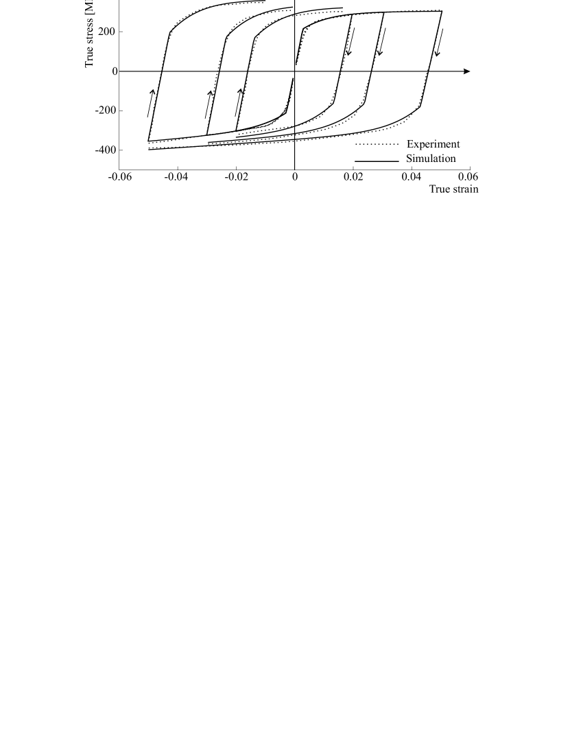
Figure 4: Uniaxial tension-followed-by-compression and compression-followed-by-tension tests. Experimental data for the cast A356 aluminium alloy (Horstemeyer, 1998) are shown by dotted lines. Simulation results are depicted by solid lines.

Table 3: Material parameters.

parameter	value	brief explanation
$k_{0}$	73500 MPa	initial bulk modulus
$\mu_{0}$	28200 MPa	initial shear modulus
$c_{0}$	6399.8 MPa	kinematic hardening parameter
$\varkappa_{0}$	0.015106 MPa-1	kinematic hardening parameter
$\gamma_{0}$	1442.2 MPa	isotropic hardening parameter
$\beta_{0}$	1.852	isotropic hardening parameter
$K_{0}$	210 MPa	initial yield stress
$m$	1	viscosity parameter
$\eta$	100 s	viscosity parameter
KRR	67.63	kinematic hardening reduction rate
IRR	29.97	isotropic hardening reduction rate
BRR	45	bulk modulus reduction rate
SRR	30	shear modulus reduction rate
$v_{\text{tens}}$	$10^{-7}$ $\text{mm}^{3}$	void volume nucleated under tension
$v_{\text{shear}}$	$10^{-7}$ $\text{mm}^{3}$	void volume nucleated under shear
$n_{\text{tens}}$	2773000 $\text{mm}^{-3}\text{MPa}^{-1}$	void nucleation parameter (tension)
$K_{\text{tens}}$	0.79	void nucleation parameter (tension)
$n_{\text{shear}}$	17188000 $\text{mm}^{-3}\text{MPa}^{-1}$	void nucleation parameter (shear)
$K_{\text{shear}}$	0.9353	void nucleation parameter (shear)
$n_{\text{comp}}$	0 $\text{mm}^{-3}\text{MPa}^{-1}$	void nucleation parameter (compression)
$f_{0}$	1 MPa	constant (not a material parameter)

For the validation of the material model, a series of numerical tests is performed. As the reference configuration we choose the initial configuration occupied by the body at $t=0$. Since the initial state is stress free, we put $\accentset{\text{por}}{\mathbf{C}}_{\text{i}}|_{t=0}=\mathbf{1}$. Furthermore, the initial state of the cast material is assumed to be isotropic. Therefore, we have $\accentset{\text{por}}{\mathbf{C}}_{\text{ii}}|_{t=0}=\mathbf{1}$. The remaining initial conditions are given by $s|_{t=0}=s_{\text{d}}|_{t=0}=0$, $\Phi|_{t=0}=1$.

We define the set of material parameters as follows. Firstly, void growth is neglected here: $d_{\text{growth}}=0$. Moreover, we neglect void nucleation under compression by putting $n_{\text{comp}}=0$. Thus, the values of $K_{\text{comp}}$ and $v_{\text{comp}}$ become irrelevant. The elasticity parameters $k_{0}$ and $\mu_{0}$ are identified using the stress-strain curve in the elastic range. The initial yield stress $K_{0}$ is estimated at a transition from elasticity to plasticity under quasistatic loading conditions. In general, the viscosity parameters $m$ and $\eta$ can be estimated using a series of tests with different loading rates. In this section we neglect the real viscous effects and adopt the parameters $m$ and $\eta$ only as numerical regularization parameters. All simulations will be performed with a low loading rate such that the overstress $f$ will remain below $10$ MPa. Next, the nucleation parameters $K_{\text{tens}}$, $K_{\text{shear}}$, $n_{\text{tens}}$, and $n_{\text{shear}}$ should be identified by counting the void nucleation sites as a function of strain under different loading conditions (Horstemeyer et al., 2000). In this section, $v_{\text{tens}}$ and $v_{\text{shear}}$ are roughly estimated by assuming that each void has a volume of approximately $10^{-7}\text{mm}^{3}$. In general, the parameters $v_{\text{tens}}$ and $v_{\text{shear}}$ should be identified by measuring the volume changes induced by ductile damage. Finally, the remaining parameters can be reliably identified using the experimental flow curves shown in Figure 4. Note that only 7 material parameters ($K_{0}$, $\gamma_{0}$, $\beta_{0}$, $\varkappa_{0}$, $c_{0}$, IRR, KRR) were adjusted to fit the flow curves. The set of material parameters which is used to describe the material response is summarized in Table 3.

The stress response of the material can be described by the proposed material model with sufficient accuracy (cf. Figure 4). Within the numerical simulation, the real Bauschinger effect is slightly underestimated, which leads to a minor discrepancy between the simulated and the real stress responses shortly after the secondary yielding. Following the ideas of Chaboche (1989), this discrepancy can be reduced by introducing additional backstress.

During the phase of 5% prestrain under tension (within the tension-followed-by-compression test), the theoretical value of $\Phi$ can be up to $\Phi_{0.05}=1.00428$. The elastic modulus $E_{0.05}$ following 5% tension and the initial modulus $E_{0}$ are computed with

$$E_{0.05}=\frac{9k(\Phi_{0.05})\ \mu(\Phi_{0.05})}{3k(\Phi_{0.05})+\mu(\Phi_{0.05})},\quad E_{0}=\frac{9k_{0}\ \mu_{0}}{3k_{0}+\mu_{0}}.$$ (90)

The numerical simulation yields $E_{0.05}=0.8729\ E_{0}$, which corresponds to $12.7\%$ reduction. At the same time, the elastic modulus is unaffected by the 5% compression. As can be seen from Figure 4, the elastic unloading is captured by the model with ample accuracy, both for tensional and compressional prestrains.

Another noteworthy aspect is the following. According to Table 3, KRR $\approx$ 2 IRR. This means that the deterioration of the kinematic hardening progresses twice as fast as the deterioration of the isotropic hardening. Thus, the concept of effective stresses combined with the strain equivalence principle is too restrictive for the cast A356 aluminium alloy, since this concept implies that the kinematic and isotropic hardening deteriorate with the same rate (Grammenoudis et al., 2009; Bröcker and Matzenmiller, 2014).

Uniaxial experiments are insufficient to validate the void nucleation rule proposed in the current study. Such a validation should be based on experimental observation of void nucleation for different loading conditions. In this study we use experimental data previously reported by Horstemeyer et al. (2000) for the cast A356 aluminium alloy, see Figure 5 (left). Tension and torsion are considered here. The simulated void number $N$ is plotted versus the accumulated inelastic arc-length $s$ in Figure 5 (right). For the simulation of both tests, the initial value of 15000 voids per $\text{mm}^{3}$ is adopted. The simulation results correspond qualitatively to the experimental data.

\psfrag{A}[m][1][0]{$N/\text{mm}^{3}$}\psfrag{S}[m][1][0]{$s$}\psfrag{B}[m][1][0]{$\#/\text{mm}^{2}$}\includegraphics{Fig5.eps}

Figure 5: Left: Experimental results for the void nucleation in the cast A356 aluminium alloy (Horstemeyer et al., 2000). Number of voids per unit area is depicted. Right: Simulation results for the void number $N$ as a function of the accumulated inelastic arc-length $s$. Depending on the choice of the material parameters, the void nucleation rate under shear may exceed the nucleation rate under tension.

5 FEM solution of a representative boundary value problem

An axisymmetric deep drawing of a circular sheet metal blank is considered in this section to demonstrate the applicability of the new model and to test the stability of the implemented numerical procedures. The setup is depicted in Fig. 6.

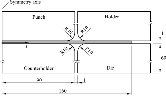
Figure 6: Setup of the axisymmetric deep drawing.

The overall forming process consists of three steps:

• Preliminary step: Forces are gradually applied both to holder and counterholder.

• Deep drawing: The punch pushes the blank into the die.

• Spring back: The blank is released from any contact.

The material of the blank is described by the proposed material model with parameters taken from Table 3, which correspond to the A356 aluminium alloy. The remaining bodies are assumed to be rigid. Coulomb friction is assumed with a friction coefficient of 0.1. A quasistatic loading rate is chosen such that the kinetic energy is negligible compared to the work of external forces. Mass scaling, which is typically adopted to speed up computation, is not used here. The FE mesh consists of 1950 elements of ABAQUS type CAX4R (4-node bilinear axisymmetric quadrilateral element with reduced integration, hourglass control, linear geometric order). Steps 1, 2 and 3 last $0.01\text{s}$, $0.10\text{s}$ and $0.12\text{s}$, respectively. The simulation required $460\,563$, $4\,638\,783$ and $5\,592\,654$ increments for steps 1, 2 and 3, respectively.

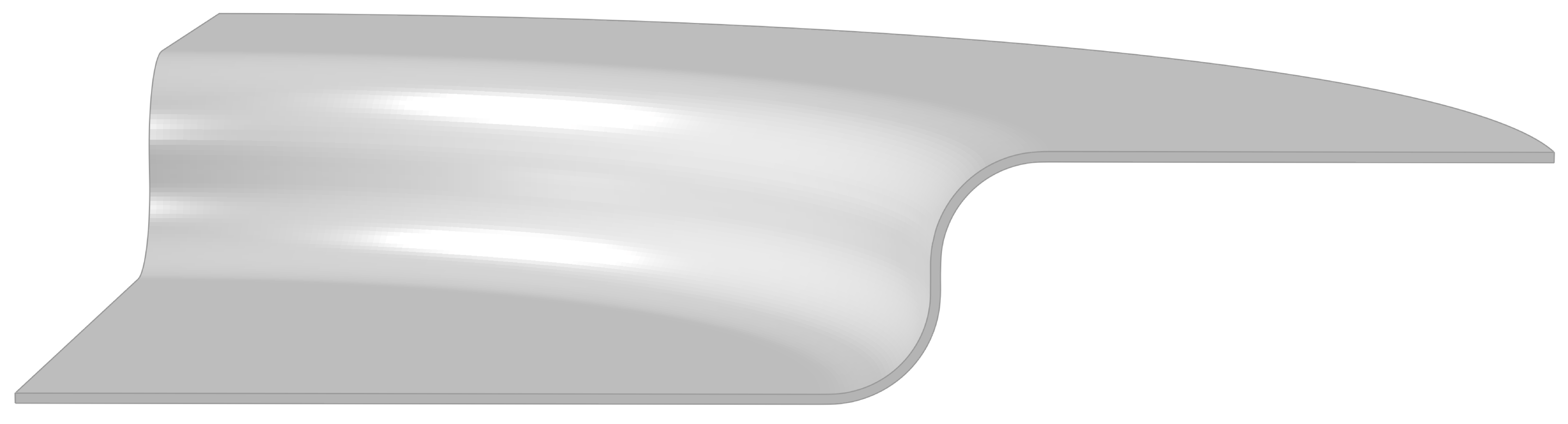
Figure 7: Deformed state after deep drawing. Only a quarter of the blanket is shown.

It is known that the deterioration of elastic properties and the Bauschinger effect have a strong impact on the spring back (Wagoner et al., 2013). The deformed state after deep drawing is shown in Fig. 7. Fig. 8 shows the distribution of the von Mises equivalent stress after deep drawing and after the spring back. Fig. 9 provides the distribution of the maximum and minimum principal stresses after the spring back. Note that the residual stresses remain high compared to the initial yield stress ($K_{0}=210\ \text{MPa}$).

\psfrag{A}[m][1][0]{after deep drawing}\psfrag{B}[m][1][0]{after spring back}\psfrag{C}[m][1][0]{von Mises stresses}\includegraphics{Fig8.eps}

Figure 8: Distribution of von Mises stresses after deep drawing (left) and after spring back (right).

\psfrag{A}[m][1][0]{maximum principal stress}\psfrag{B}[m][1][0]{minimum principal stress}\includegraphics{Fig9.eps}

Figure 9: Distribution of maximum and minimum principal stresses after the spring back.

\psfrag{A}[m][1][0]{inelastic arc length $s$}\psfrag{B}[m][1][0]{damage measure $\Phi-1$}\includegraphics{Fig10.eps}

Figure 10: Distribution of the inelastic arc length $s$ (left) and damage measure $\Phi-1$ (right) after the spring back.

By comparison with the resulting inelastic arc length field $s$ (cf. Fig. 10 (left)), it becomes clear that highest residual stresses appear in regions with a considerable gradient of $s$. The distribution of the damage measure $\Phi-1$ after spring back is depicted in Fig. 10 (right). Note that $\Phi-1$ remains in the range of a few percent and the damage is concentrated in the deep-drawn section. The observed damage hot spots are considered as a precursor of failure.

Note that a generic local approach to ductile damage is adopted in this study. In general, the simulation results for local damage models are pathologically mesh-dependent in case of localizing deformation processes. Thus, the presented model should not be used for the analysis of post-localization structural behavior. The post-localization analysis should be based on nonlocal damage models which enrich the continuum formulation by introducing a physics-based length scale (see Bažant and Jirásek (2002); Anand et al. (2012); Ahad et al. (2014); Nguyen et al. (2015) and references therein). Some sort of regularization is also possible using the viscosity, which is available in the current model. Unfortunately, this technique is effective only in a narrow range of deformation rates (Bažant and Jirásek, 2002). Still, the proposed local material model is useful for estimating the process parameters which lead to undesired strain localization. No strain localization was observed in the current simulation.

6 Discussion and conclusion

A thermodynamically consistent approach to ductile damage and nonlinear kinematic hardening is suggested within the framework of multiplicative plasticity. It is well established that at the early stage of the damage process the damage is adequately described by the scalar porosity variable (see, for example, Tvergaard (1989)). Thus, for simplicity, isotropic damage with no prominent orientation is assumed in this study. To extend the current model to the case of anisotropic damage, some physics-based tensorial damage quantities can be introduced.

The damage-induced volume change is taken into account explicitly by the model kinematics for the accurate prediction of the hydrostatic stress component. Another feature of the proposed model is that isotropic and kinematic hardening deteriorate differently for increasing damage, which is essential for an accurate description of the real material response. Moreover, the deterioration of elastic properties is introduced for the correct prediction of residual stresses and spring back. Next, a refined void nucleation rule is constructed in this study aiming at accurate description of the complex behavior of porous ductile metals with second phases. In particular, the new rule is suitable for materials which exhibit a higher void nucleation rate under torsion than in case of tension. The proposed model is validated using the experimental observations of the void nucleation under various loading conditions and experimental stress-strain curves. These curves carry information on the evolution of plastic anisotropy, reduction of strain hardening capacity, and deterioration of elastic properties.

The phenomenological formulation can be enriched by physics-based rules for void nucleation, growth and coalescence. The restrictions imposed on these relations by the Clausius-Duhem inequality are obtained in an explicit form. Interestingly, a cut-off value for hydrostatic pressure is obtained from irreversible thermodynamics in a natural way (cf. $\eqref{RestricOnPhi}_{2}$).

A relatively large number of material parameters is introduced due to a variety of nonlinear phenomena covered by the model. In some applications, however, certain parts of the model can be switched off to reduce the number of parameters. For instance, some elementary or classical void nucleation rules can be adopted (cf. Appendix A). Alternatively, the nucleation rules (55) – (57) can be calibrated using experiments (cf. Su et al. (2010) ) or lower-scale models (cf. Gall et al. (2000); Dandekar and Shin (2011)).

An efficient hybrid explicit/implicit numerical procedure is presented. This procedure exhibits increased stability and accuracy being compared to a purely explicit time stepping. The feasibility of the proposed algorithm is tested numerically and the algorithm is shown to be suitable for explicit FEM analysis.

Although the model has been developed for forming simulations, another promising application includes the prediction of damage and plastic anisotropy in ultra-fine grained materials produced by severe plastic deformations (Wagner et al., 2010; Frint et al., 2011; Neugebauer et al., 2012). An extension of the framework to models of creep damage mechanics (Altenbach et al., 2002; Altenbach, 2003) is possible as well.

Appendix A (some void nucleation rules)

In this appendix we briefly recall some of the void nucleation rules that are available in the literature. For simplicity, only monotonic loading is considered here. Let $N$ be the void number per unit volume of the reference configuration. A very simple void nucleation rule says that $N$ is a linear function of the accumulated plastic arc-length $s$ (Gurland, 1972)

$$\dot{N}=\lambda_{\text{i}}\ n_{\text{Gurland}}\quad\stackrel{{\scriptstyle\eqref{evol2}}}{{\Rightarrow}}\quad\frac{\displaystyle\partial N}{\displaystyle\partial s}=\sqrt{3/2}\ n_{\text{Gurland}}.$$ (91)

Here, $n_{\text{Gurland}}\geq 0$ is a material parameter. In other words, the void nucleation rate $\frac{\partial N}{\partial s}$ is assumed to be independent of the stage of the deformation process and of the stress state.

In order to capture the dependence on the stage of the deformation process, relation (91) was generalized by Gurson (1977). Here we consider a popular modification of Gurson’s rule. Let $f_{\text{void}}$ be the void volume fraction. For the strain-controlled nucleation, Chu and Needleman (1980) assumed that the void nucleation is governed by a normal distribution law

$$\dot{f}_{\text{void}}=\frac{f_{\text{N}}}{S_{\text{N}}\sqrt{2\pi}}\exp\Big{[}-\frac{\displaystyle 1}{\displaystyle 2}\Big{(}\frac{s-s_{\text{N}}}{S_{\text{N}}}\Big{)}^{2}\Big{]}\ \dot{s},$$ (92)

where $f_{\text{N}},S_{\text{N}},s_{\text{N}}\geq 0$ are material parameters; $s$ denotes the accumulated plastic arc-length. Note that (91) can be approximated by (92) with large $f_{\text{N}}$ and $S_{\text{N}}$ and by assuming that $\dot{f}_{\text{void}}$ is proportional to $\dot{N}$. Another modification of Gurson’s rule was proposed by Chu and Needleman (1980) for stress-controlled nucleation.

Rule (92) is sufficiently accurate for some alloys (Chen and Worswick, 2008). However, in ductile metals with second phases, a complex dependence of void nucleation on the stress state can be observed. For instance, torsion induces a higher void nucleation rate than tension in the cast A356 aluminum (Horstemeyer et al., 2000). In order to account for this effect, the following void nucleation rule was proposed by Horstemeyer and Gokhale (1999). First, recall that $\hat{\mathbf{\Sigma}}$ is the effective stress tensor. Let $J_{2}$ and $J_{3}$ be the invariants of the deviatoric part $\hat{\mathbf{\Sigma}}^{\text{D}}$. The hydrostatic stress component is captured by $\text{tr}\hat{\mathbf{\Sigma}}$. The void nucleation is governed by

$$\dot{N}=\lambda_{\text{i}}\ N\ \Bigg{[}p_{1}\Big{(}\frac{4}{27}-\frac{J^{2}_{3}}{J^{3}_{2}}\Big{)}+p_{2}\frac{J_{3}}{J^{3/2}_{2}}+p_{3}\frac{|\text{tr}\hat{\mathbf{\Sigma}|}}{J^{1/2}_{2}}\Bigg{]},$$ (93)

where $p_{1}$, $p_{2}$ and $p_{3}$ are material parameters.

Appendix B (discussion of void nucleation rules)

Table 4: Qualitative analysis of the void nucleation rules.

Nucleation rule	Equa-	Asymptotic	Role of hydro-	Increased nucl. rate
	tion	behavior	static stress	under torsion
Gurland (1972)	(91)	linear growth	irrelevant	impossible
Chu and Needleman (1980)	(92)	saturation	irrelevant	impossible
Horstemeyer and	(93)	exponential	sign of hydrostatic	possible
Gokhale (1999)		growth	stress is irrelevant
New rule (current study)	(53) –	linear growth	sensitive to	possible
	– (57)		hydrostatic stress

Let us compare the void nucleation rules presented in Appendix A with the new rule introduced in Section 2.6. This comparison is based on different criteria, such as the saturation of the void number under monotonic loading, the role played by the hydrostatic stress component, and the increased nucleation rate under torsion compared to tension.

Saturation: It is usually assumed that the voids nucleate at certain inclusions, or, more generally, at second phases which are sites of local stress raisers. Thus, the total number of voids is limited by the number of inclusions of a certain type. Gurland’s rule (cf. (91)) predicts a linear accumulation of voids, without any saturation. A nearly linear void accumulation is also predicted by the newly constructed relations (53) – (57) (cf. Figure 5). If needed, the saturation can be introduced by a simple modification, which is not considered in the current study. Next, the rule from Chu and Needleman (cf. (92)) is realistic in the sense that the maximum void volume fraction is bounded due to the saturation of the void nucleation. Finally, the rule from Horstemeyer and Gokhale (cf. (93)) predicts even an accelerated void nucleation. More precisely, the void number under monotonic loading increases exponentially. Interestingly, the rule from Horstemeyer and Gokhale says that no voids can be created in initially void-free material. Indeed, if $N|_{t=0}=0$ then (93) yields $N\equiv 0$.

The role of hydrostatic stress: The influence of the hydrostatic stress component is neglected by both (91) and (92). In contrast to this, the new nucleation rule (55) is highly sensitive to $\text{tr}\hat{\mathbf{\Sigma}}$ such that for larger hydrostatic stresses increased nucleation rates are predicted. Interestingly, the rule from Horstemeyer and Gokhale (cf. (93)) operates with the absolute value of the hydrostatic stress component $|\text{tr}\hat{\mathbf{\Sigma}}|$. Thus, the sign of $\text{tr}\hat{\mathbf{\Sigma}}$ is irrelevant!

Increased nucleation rate under torsion: As already mentioned above, torsion may induce a higher void nucleation rate than tension. The classic rules from Gurland as well as Chu and Needleman cannot describe this effect. By appropriate choice of material parameters, the rule from Horstemeyer and Gokhale and the new rule introduced in Section 2.6 are capable of reproducing this type of behavior. Note that different systems of invariants are used in these rules.

The theoretical results are summarized in Table 4. In conclusion, note that the assumption of linear growth of the void number is compatible with the experimental data available for the cast A356 aluminium (see Figure 5).

References

- Ahad et al. (2014) Ahad, F.R., Enakoutsa, K., Solanki, K.N., Bammann, D.J., 2014. Nonlocal modeling in high-velocity impact failure of 6061-T6 aluminum. International Journal of Plasticity 55, 108–132.
- Altenbach et al. (2002) Altenbach, H., Huang, C., Naumenko, K., 2002. Creep-damage predictions in thin-walled structures by use of isotropic and anisotropic damage models. Journal of Strain Analysis for Engineering Design 37(3), 265–275.
- Altenbach (2003) Altenbach, H., 2003. Topical problems and applications of creep theory. International Applied Mechanics 39(6), 631–655.
- Anand et al. (2012) Anand, L., Aslan, O., Chester, S.A., 2012. A large-deformation gradient theory for elastic-plastic materials: Strain softening and regularization of shear bands. International Journal of Plasticity 30–31, 116–143.