Collective Hamiltonian for wobbling modes

Abstract

The simple, longitudinal, and transverse wobblers are systematically studied within the framework of collective Hamiltonian, where the collective potential and mass parameter included are obtained based on the tilted axis cranking approach. Solving the collective Hamiltonian by diagonalization, the energies and the wave functions of the wobbling states are obtained. The obtained results are compared with those by harmonic approximation formula and particle rotor model. The wobbling energies calculated by the collective Hamiltonian are closer to the exact solutions by particle rotor model than harmonic approximation formula. It is confirmed that the wobbling frequency increases with the rotational frequency in simple and longitudinal wobbling motions while decreases in transverse wobbling motion. These variation trends are related to the stiffness of the collective potential in the collective Hamiltonian.

I Introduction

Atomic nuclei possess a wide variety of shapes in both their ground and excited states. The shapes may range from spherical to deformed, from quadrupole to octupole, and even more exotic shapes, such as superdeformed and tetrahedral. For deformed nuclei, they in general possess axially symmetric shape. The loss of axially symmetry would lead to triaxial shape. The triaxiality has been invoked to describe many interesting phenomena including $\gamma$-band Bohr and Mottelson (1975), signature inversion Bengtsson et al. (1984), anomalous signature splitting Hamamoto and Sagawa (1988), chiral symmetry breaking Frauendorf and Meng (1997); Frauendorf (2001); Meng and Zhang (2010), and the wobbling motion Bohr and Mottelson (1975). The wobbling motion and chirality are regarded as fingerprints of stable triaxial nuclei.

The wobbling motion within nuclear rotation was originally introduced by Bohr and Mottelson Bohr and Mottelson (1975) in the context of the triaxial rotor model (TRM). For a rotating triaxial even-even nuclei, the rotation motions about any of axes are all possible and the corresponding TRM Hamiltonian reads

$$\hat{H}_{\rm rot}=\frac{\hat{I}_{1}^{2}}{2\mathcal{J}_{1}}+\frac{\hat{I}_{2}^{2}}{2\mathcal{J}_{2}}+\frac{\hat{I}_{3}^{2}}{2\mathcal{J}_{3}},$$ (1)

with three distinct moments of inertia $\mathcal{J}_{k}$ (usually defines $\mathcal{J}_{1}$ as maximal) associating with each of the principle axes. It is pointed out that although the triaxial nucleus energetically favors the rotation about the axis with the largest moment of inertia (i.e., $1$-axis), contributions from rotations about the other two axes ($2$ and $3$ axes) would quantum mechanically disturb this rotation and force the angular momentum vector off the $1$-axis. As a consequence, besides the uniform rotation about $1$-axis, there is wobbling motion Bohr and Mottelson (1975). The energies of wobbling states, characterized by the wobbling phonon number $n$ together with total angular momentum $I$, are

$$E(n,I)=\frac{I(I+1)}{2\mathcal{J}_{1}}+(n+\frac{1}{2})\hbar\Omega_{\rm wob}.$$ (2)

The quantum number $n$ describes the wobbling motion of the axes with respect to the direction of $I$. For small amplitudes, this motion has the character of a harmonic vibration with wobbling frequency given by

$$\hbar\Omega_{\rm wob}=2I\sqrt{\Big{(}\frac{\hbar^{2}}{2\mathcal{J}_{2}}-\frac{\hbar^{2}}{2\mathcal{J}_{1}}\Big{)}\Big{(}\frac{\hbar^{2}}{2\mathcal{J}_{3}}-\frac{\hbar^{2}}{2\mathcal{J}_{1}}\Big{)}},$$ (3)

which is related to the moments of three axes and found to be proportional to the spin. Similar as Ref. Frauendorf and Dönau (2014), such type of wobbling motion for a triaxial rotor is also denoted as “simple wobbler” at the present investigation.

The wobbling motion appears not only in the even-even nuclei but also in the odd-$A$ nuclei. For rotating odd-$A$ triaxial nuclei, there are two types of wobbling motions suggested by Frauendorf and Dönau Frauendorf and Dönau (2014) very recently according to the relation between the orientation of quasiparticle angular momentum vector with respect to the rotor axis with the largest moment of inertia. If the quasiparticle angular momentum vector is aligned with the axis with the largest moment of inertia, it is called “longitudinal wobbler”. If the quasiparticle angular momentum vector is perpendicular to the axis with the largest moment of inertia, it is called “transverse wobbler”. Assuming frozen alignment of the quasiparticle with one of the rotor axes and harmonic oscillations (HFA), a rather simple analytic expression for wobbling frequency of these two types of wobbling motions is derived Frauendorf and Dönau (2014). According to this analytic expression, the increasing trend of wobbling frequency for longitudinal wobbling motion and decreasing trend for transverse wobbling can be expected.

On the experimental side, although the wobbling phenomenon has been predicted for a long time Bohr and Mottelson (1975), it was not observed until the beginning of this century when the first experimental evidence was reported in ¹⁶³Lu Ødegård et al. (2001). Subsequently, it has been extensively studied in the triaxial strongly deformed (TSD) region around $N=94$, where the wobbling bands have been identified in ${}^{161,163,165,167}\rm Lu$ Jensen et al. (2002a, b); Schönwaßer et al. (2003); Bringel et al. (2005); Amro et al. (2003); Hagemann (2004) and ${}^{167}\rm Ta$ Hartley et al. (2009). All wobbling bands in this mass region are based on $\pi i_{13/2}$ configuration. Very recently, a new candidate wobbling band is proposed in ${}^{135}\rm Pr$ Frauendorf and Dönau (2014), which is built on $\pi h_{11/2}$ configuration, differing from the configuration of previous known examples. For even-even nuclei, however, the wobbling spectra are scarce since stable triaxial ground states are rare. The best example identified so far is ${}^{112}\rm Ru$ Zhu et al. (2009).

On the theoretical side, the wobbling motion was firstly investigated by TRM Bohr and Mottelson (1975). Following the discovery of the first wobbling structure in odd-$A$ ${}^{163}\rm Lu$ Ødegård et al. (2001), the quantal particle rotor model (PRM) was used to describe the wobbling mode, see Refs. Hamamoto (2002); Hamamoto and Mottelson (2003); Tanabe and Sugawara-Tanabe (2006, 2008); Frauendorf and Dönau (2014). Based on the framework of mean field theory, there are many efforts to extend the cranking model to study the wobbling motion. Due to the mean-filed approximation, cranking model yields only the yrast sequence for a given configuration, Therefore, in order to describe the wobbling excitations, one has to go beyond the mean-filed approximation. At present, this has been done by incorporating the quantum correlations by means of random phase approximation (RPA) Shimizu and Matsuzaki (1995); Matsuzaki et al. (2002, 2003); Matsuzaki and Ohtsubo (2004); Matsuzaki et al. (2004); Shimizu et al. (2005, 2008); Shoji and Shimizu (2009) or by the generator coordinate method after angular momentum projection (GCM+AMP) based on the cranking intrinsic states Oi et al. (2000).

Another promising method is to construct a collective Hamiltonian on the top of cranking mean field solutions. By taking into account the quantum fluctuation along the collective degree of freedom, the collective Hamiltonian goes beyond the mean-field approximation and restores the broken symmetry Chen et al. (2013). This has been implemented based on the framework of tilted axis cranking (TAC) single-$j$ shell model to investigate the chiral vibration and rotation motions Mukhopadhyay et al. (2007); Qi et al. (2009). The chiral symmetry broken in the intrinsic reference frame is restored and chiral doublet bands are obtained in the laboratory reference frame. For wobbling motion, the wobbling states are formed due to the quantum fluctuation of the total angular momentum deviating from the principle axes of the rotor. It is thus interesting to extend the collective Hamiltonian to describe the phenomenon of wobbling motion.

In this work, the collective Hamiltonian will be extended to study the simple, longitudinal, and transverse wobbling motions, in particular, to examine the trend of the wobbling frequency with respect to the rotational frequency. In the collective Hamiltonian, the collective potentials are calculated from TAC model and the mass parameter is obtained with the assumption of harmonic approximation (HA) for simple wobbling motion or HFA approximation for longitudinal and transverse wobbling motions. The energy levels and wave function of wobbling states are obtained by diagonalizing the collective Hamiltonian. The corresponding energy spectra will be in comparison with the results obtained by HA (HFA) analytic expression as well as TRM (PRM) for simple (longitudinal and transverse) wobbling to evaluate the accuracy of the collective Hamiltonian.

The paper is organized as follows. In Sec. II, a brief introduction to the collective Hamiltonian is given. The corresponding numerical details adopted in the calculations are presented in Sec. III. In Sec. IV, the obtained potential energy and the mass parameter are respectively shown for the three types of wobbling motions and the corresponding energy levels and wave functions obtained by collective Hamiltonian are discussed in details. A brief summary is given in Sec. V.

II Theoretical framework

The collective Hamiltonian, in terms of a few numbers of collective coordinates and momenta, is an effective method for describing various collective processes which involve small velocities. The well-known Bohr Hamiltonian describe the collective rotational and vibrational degrees of freedom with the five collective intrinsic variables $\beta$, $\gamma$, and Euler angles $\bm{\Omega}$ Bohr and Mottelson (1975). In Ref. Chen et al. (2013), to describe the chiral motions in triaxial rotational nuclei, a collective Hamiltonian based on the TAC solutions was constructed. Therein, the orientation of nucleus in rotating mean-field, described by polar angle $\theta$ and azimuth angle $\varphi$ in the spherical coordinate as illustrated in Fig. 1, is considered as collective variable. As the motion along $\varphi$ direction is much easier than $\theta$ direction, the collective Hamiltonian has been restricted to one dimensional motion along $\varphi$ direction Chen et al. (2013).

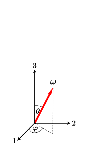
Figure 1: (Color online) Orientation of the rotational frequency $\bm{\omega}$ with respect to the principal axes.

For the wobblers caused by the quantum fluctuation of the total angular momentum orientation, the azimuth angle $\varphi$ can also be taken as collective coordinate to the wobbling motions and the wobbling excitation is restricted to one dimensional motion along $\varphi$ direction. It is necessary to mention that in a semi-classical model for wobbling motion, the azimuth angle $\varphi$ has been interpreted as the wobbling angle of the total angular momentum vector Oi (2006).

The detailed theoretical framework of collective Hamiltonian based on the TAC solutions has been formulated in Ref. Chen et al. (2013). The formalism can be analogized to describe the wobbling motion. Here for completeness, a brief introduction to the formalism is presented.

II.1 Collective Hamiltonian

Taking $\varphi$ as the collective variable, the classical form of collective Hamiltonian is written as the sum of kinetic and potential terms

$$H_{\rm coll}=T_{\rm kin}(\varphi)+V(\varphi)=\displaystyle\frac{1}{2}B(\varphi)\dot{\varphi}^{2}+V(\varphi),$$ (4)

where $V(\varphi)$ is collective potential and $B(\varphi)$ mass parameter. The quantized form of the collective Hamiltonian is obtained according to the Pauli prescription Pauli (1933)

$$\hat{H}_{\rm coll}=-\displaystyle\frac{\hbar^{2}}{2\sqrt{B(\varphi)}}\frac{\partial}{\partial\varphi}\frac{1}{\sqrt{B(\varphi)}}\frac{\partial}{\partial\varphi}+V(\varphi).$$ (5)

By solving this Hamiltonian on the basis states with appropriate boundary condition on $\varphi$, e.g., box boundary condition Chen et al. (2013), the wobbling levels and corresponding wave functions can be obtained.

II.2 Collective potential $V(\varphi)$

Both the collective potential $V(\varphi)$ and the mass parameter $B(\varphi)$ in the collective Hamiltonian (4) can be determined based on TAC model.

Let us first discuss $V(\varphi)$ for the cases of longitudinal and transverse wobblers. For schematic discussions, we consider a system of a high-$j$ particle coupled to a triaxial rotor. The cases for more than one particle coupled to triaxial rotor can be easily extended as well. The cranking Hamiltonian reads

$$\hat{h}^{\prime} =\hat{h}_{\rm def}-\bm{\omega}\cdot\hat{\bm{j}},$$

$$\bm{\omega} =(\omega\sin\theta\cos\varphi,\omega\sin\theta\sin\varphi,\omega\cos\theta),$$ (6)

where $\hat{\bm{j}}$ is the single particle angular momentum and deformed single particle Hamiltonian $\hat{h}_{\rm def}$ is taken as the single-$j$ shell Hamiltonian

$$\hat{h}_{\rm def}=\frac{1}{2}C\Big{\{}(\hat{j}_{3}^{2}-\frac{j(j+1)}{3})\cos\gamma+\frac{1}{2\sqrt{3}}(\hat{j}_{+}^{2}+\hat{j}_{-}^{2})\sin\gamma\Big{\}}.$$ (7)

Diagonalizing the cranking Hamiltonian, one obtains the total Routhian

$$E^{\prime}(\theta,\varphi)=\langle h^{\prime}\rangle-\frac{1}{2}\sum_{k=1}^{3}\mathcal{J}_{k}\omega_{k}^{2},\quad\mathcal{J}_{k}:\textrm{moments of inertia},$$ (8)

Minimizing the total Routhian with respect to $\theta$ for given $\varphi$, the collective potential $V(\varphi)$ is finally obtained.

For simple wobbler, i.e., a simple triaxial rotor without coupling any particles, the total Routhian (8) is degenerated to

$$E^{\prime}(\theta,\varphi)=-\frac{1}{2}\sum_{k=1}^{3}\mathcal{J}_{k}\omega_{k}^{2},$$ (9)

and similarly the collective potential $V(\varphi)$ is obtained by minimizing the total Routhian with respect to $\theta$ for given $\varphi$.

II.3 Mass parameter $B$

Before discussing how to calculate the mass parameter, it is worth noting once more that as pointed out by Bohr and Mottelson Bohr and Mottelson (1975), the wobbling motion as a small amplitude vibration has the character of a harmonic oscillation with frequency $\Omega_{\rm wob}$. As well-known, the oscillation frequency $\Omega$ for a harmonic oscillator system is related to the mass parameter $B$ of the oscillator and the stiffness parameter $C$ of the harmonic oscillator potential by

$$\Omega=\sqrt{\frac{C}{B}}.$$ (10)

Therefore, once the stiffness parameter $C$ and oscillation frequency $\Omega$ are determined, the mass parameter $B$ can be obtained.

To extract the stiffness parameter $C$ of the collective potential $V(\varphi)$, one can expand the collective potential $V(\varphi)$ by Taylor series at $\varphi=0^{\circ}$ up to $\sim\varphi^{2}$ terms, i.e., the harmonic approximation (HA) is adopted. For the total Routhian (9) of simple wobbler, one can find that its minimum along $\theta$ direction is always at $\theta=90^{\circ}$ for any value of $\varphi$. Therefore, the collective potential becomes

$$V(\varphi) =-\frac{1}{2}\omega^{2}(\mathcal{J}_{1}\cos^{2}\varphi+\mathcal{J}_{2}\sin^{2}\varphi)$$ (11)

$$\approx-\frac{1}{2}\mathcal{J}_{1}\omega^{2}+\frac{1}{2}\omega^{2}(\mathcal{J}_{1}-\mathcal{J}_{2})\varphi^{2},\quad\quad\textrm{for $\varphi\to 0^{\circ}$}.$$ (12)

The Eq. (12) suggests that the collective potential can be regarded as the sum of a rotational energy term along 1-axis with frequency $\omega$ and a harmonic oscillation potential term along $\varphi$ direction with stiffness parameter $C=\omega^{2}(\mathcal{J}_{1}-\mathcal{J}_{2})$. Thus the wobbling frequency $\Omega_{\rm wob}$ and the mass parameter $B$ are related each other by

$$\hbar\Omega_{\rm wob}=\hbar\sqrt{\frac{C}{B}}=\hbar\omega\sqrt{\frac{\mathcal{J}_{1}-\mathcal{J}_{2}}{B}}.$$ (13)

To determine the mass parameter $B$ in Eq. (13), we further recall the wobbling frequency (3) given by Bohr and Mottelson Bohr and Mottelson (1975)

$$\hbar\Omega_{\rm wob} =2I\sqrt{\Big{(}\frac{\hbar^{2}}{2\mathcal{J}_{2}}-\frac{\hbar^{2}}{2\mathcal{J}_{1}}\Big{)}\Big{(}\frac{\hbar^{2}}{2\mathcal{J}_{3}}-\frac{\hbar^{2}}{2\mathcal{J}_{1}}\Big{)}}$$

$$=\frac{\hbar^{2}I}{\mathcal{J}_{1}}\sqrt{\frac{(\mathcal{J}_{1}-\mathcal{J}_{2})(\mathcal{J}_{1}-\mathcal{J}_{3})}{\mathcal{J}_{3}\mathcal{J}_{2}}}$$

$$=\hbar\omega\sqrt{\frac{(\mathcal{J}_{1}-\mathcal{J}_{2})(\mathcal{J}_{1}-\mathcal{J}_{3})}{\mathcal{J}_{3}\mathcal{J}_{2}}}.$$ (14)

Combining Eqs. (13) and (II.3), the mass parameter is obtained for simple wobbler

$$B=\frac{\mathcal{J}_{2}\mathcal{J}_{3}}{\mathcal{J}_{1}-\mathcal{J}_{3}}.$$ (15)

It is determined only by the moments of inertia of three principal axes and independent of rotational frequency.

For longitudinal and transverse wobblers, we introduce the harmonic frozen alignment (HFA) approximation as Ref. Frauendorf and Dönau (2014), i.e., the angular momentum of the odd particle is assumed to be firmly aligned with the short-axis (1-axis) and can be considered as a number. Then for a given rotational frequency $\omega$, the moment of inertia of 1-axis is treated as a $\omega$-dependent effective moment of inertia

$$\mathcal{J}_{1}^{*}(\omega)=\frac{\mathcal{J}_{1}\omega+j}{\omega}=\mathcal{J}_{1}+\frac{j}{\omega}.$$ (16)

The odd-particle contributes a $\omega$-dependent term to the effective moment of inertia, which will decrease with the increasing rotational frequency.

Similar to simple wobbler, it can be also found that for the longitudinal and transverse wobblers the collective potential obtained from the total Routhian $E^{\prime}(\theta,\varphi)$ (8) is minimized at $\theta=90^{\circ}$ for any given $\varphi$. Therefore, the collective potential is written as

$$V(\varphi) =\langle\hat{h}_{\rm def}\rangle-\omega j\cos\varphi-\frac{1}{2}\omega^{2}(\mathcal{J}_{1}\cos^{2}\varphi+\mathcal{J}_{2}\sin^{2}\varphi)$$ (17)

$$\approx\langle\hat{h}_{\rm def}\rangle-\omega j(1-\frac{\varphi^{2}}{2})-\frac{1}{2}\mathcal{J}_{1}\omega^{2}+\frac{1}{2}\omega^{2}(\mathcal{J}_{1}-\mathcal{J}_{2})\varphi^{2},\quad\quad\textrm{for $\varphi\to 0$}$$

$$=\langle\hat{h}_{\rm def}\rangle-\frac{1}{2}\omega j-\frac{1}{2}\Big{(}\mathcal{J}_{1}+\frac{j}{\omega}\Big{)}\omega^{2}+\frac{1}{2}\omega^{2}\Big{[}\Big{(}\mathcal{J}_{1}+\frac{j}{\omega}\Big{)}-\mathcal{J}_{2}\Big{]}\varphi^{2}$$

$$=\langle\hat{h}_{\rm def}\rangle-\frac{1}{2}\omega j-\frac{1}{2}\mathcal{J}_{1}^{*}\omega^{2}+\frac{1}{2}\omega^{2}\Big{[}\mathcal{J}_{1}^{*}(\omega)-\mathcal{J}_{2}\Big{]}\varphi^{2}.$$ (18)

This formula is similar to Eq. (12) except that the moment of inertia of 1-axis $\mathcal{J}_{1}$ has been replaced by the effect moment of inertia $\mathcal{J}_{1}^{*}(\omega)$, thereby one expects the mass parameter for longitudinal and transverse wobblers has the similar form as simple wobbler

$$B(\omega)=\frac{\mathcal{J}_{2}\mathcal{J}_{3}}{\mathcal{J}_{1}^{*}(\omega)-\mathcal{J}_{3}}=\frac{\mathcal{J}_{2}\mathcal{J}_{3}}{(\mathcal{J}_{1}-\mathcal{J}_{3})+\displaystyle\frac{j}{\omega}}.$$ (19)

Differing from the mass parameter (15) for simple wobbler, it is determined not only by the moments of inertia of three principal axes, but also by the angular momentum of the odd particle and the rotational frequency. As the rotational frequency increases, the mass parameter for longitudinal and transverse wobblers will increase as well.

The wobbling frequency for the longitudinal and transverse wobbling motions can be then obtained from Eq. (13)

$$\hbar\Omega_{\rm wob} =\sqrt{\frac{\mathcal{J}_{1}^{*}(\omega)-\mathcal{J}_{2}}{B(\omega)}}\hbar\omega$$

$$=\hbar\sqrt{\frac{\big{[}(\mathcal{J}_{1}-\mathcal{J}_{3})\omega+j\big{]}\big{[}(\mathcal{J}_{1}-\mathcal{J}_{2})\omega+j\big{]}}{\mathcal{J}_{2}\mathcal{J}_{3}}}.$$ (20)

This formula is nothing but the HFA formula in Ref. Frauendorf and Dönau (2014) by replacing the spin with $\mathcal{J}_{1}\omega+j$. For longitudinal wobbling motion, since $\mathcal{J}_{1}>\mathcal{J}_{2},\mathcal{J}_{3}$, the wobbling frequency increases with the rotational frequency. While for transverse wobbling motion, since $\mathcal{J}_{2}>\mathcal{J}_{1}$, the wobbling frequency decreases with the rotational frequency, and will reach to zero at a critical rotational frequency $\hbar\omega_{\rm c}=j/(\mathcal{J}_{2}-\mathcal{J}_{1})$.

III Numerical details

In the following calculations, a triaxial rotor with the deformation parameters $\beta=0.25$ and $\gamma=-30^{\circ}$ is considered to investigate the simple wobbling motion. Following the notation as in Ref. Ring and Schuck (1980), for such deformation, three principal axes $1$, $2$, and $3$-axis respectively correspond to short ($s$), intermediate ($i$), and long ($l$) axis. For the investigation of the longitudinal and transverse wobbling motions, the triaxial rotor is assumed to be further coupled with a $h_{11/2}$ proton particle. Thus the proton aligns its angular momentum along short axis (namely, 1-axis). The longitudinal (transverse) wobblers is achieved by choosing 1-axis to be (perpendicular to) the axis with largest moments of inertia.

With regard to the moments of inertia, both the rigid body type

$$\mathcal{J}_{k}^{\rm rig} =\frac{2}{5}mAR_{0}^{2}\displaystyle\Big{[}1-\sqrt{\frac{5}{4\pi}}\beta\cos(\gamma-\frac{2\pi}{3}k)\Big{]}$$

$$=\mathcal{J}_{0}^{\rm rig}\displaystyle\Big{[}1-\sqrt{\frac{5}{4\pi}}\beta\cos(\gamma-\frac{2\pi}{3}k)\Big{]},\quad k=1,2,3$$ (21)

and the irrotational flow type

$$\mathcal{J}_{k}^{\rm irr} =\frac{3}{2\pi}mAR_{0}^{2}\beta^{2}\sin^{2}(\gamma-\frac{2\pi}{3}k)$$

$$=\mathcal{J}_{0}^{\rm irr}\sin^{2}(\gamma-\frac{2\pi}{3}k),\quad k=1,2,3$$ (22)

are often assumed Ring and Schuck (1980). $\mathcal{J}_{k}^{\rm rig}$ shows less dependence on the deformation $\beta$ than $\mathcal{J}_{k}^{\rm irr}$ ($\sim\beta^{2}$). In the $\gamma$-dependence, $\mathcal{J}^{\rm irr}$ vanishes about the symmetry axes while $\mathcal{J}^{\rm rig}$ not and the largest moment of inertia axes of them are different. For the present deformation parameters $\beta=0.25$ and $\gamma=-30^{\circ}$, the largest moment of inertia axis is 1-axis ($s$-axis) for rigid body type while 2-axis ($i$-axis) for irrotational flow type.

In present investigation, the wobbling angle $\varphi$ in collective Hamiltonian is restricted to $-\pi/2\leq\varphi\leq\pi/2$, or in other words the wobbling motion happens around 1-axis. For simple wobbler, the rigid body type of moments of inertia (III) is adopted for 1-axis being the axis with the largest moment of inertia. Similarly, the rigid body type of moments of inertia is also applied to longitudinal wobbler so that the orientation of proton angular momentum (1-axis) being parallel to the axis with largest moments of inertia. For transverse wobbler, while the orientation of proton angular momentum (1-axis) is required to be perpendicular to the axis with largest moments of inertia, the irrotational flow type of moments of inertia (III) is adopted. In the calculations, the constants $\mathcal{J}_{0}^{\rm rig}$ and $\mathcal{J}_{0}^{\rm irr}$ in Eqs. (III) and (III) are respectively taken as $\mathcal{J}_{0}^{\rm rig}=256\pi/15~{}\hbar^{2}/\rm MeV$ and $\mathcal{J}_{0}^{\rm irr}=40~{}\hbar^{2}/\rm MeV$.

IV Results and discussion

IV.1 Simple wobbler

We first present the results of our calculations for the simple wobbling motion by means of the TAC model and collective Hamiltonian. As described in Sec. II, the collective potential and the mass parameter included in the collective Hamiltonian are respectively calculated by TAC model and Eq. (15). The obtained wobbling energies will be compared with the HA formula and the exact TRM.

IV.1.1 Collective potential

In contour plots of Fig. 2(a)-(d), the total Routhian $E^{\prime}(\theta,\varphi)$ (9) in the ($\theta$, $\varphi$) plane at the rotational frequencies $\hbar\omega=0.1$, $0.2$, $0.3$, and $0.4~{}\rm MeV$ are shown. All the potential energy surfaces are symmetrical with respect to $\varphi=0^{\circ}$ line. With the increasing rotational frequency, the minima in the potential energy surfaces always locate at $(\theta=90^{\circ},\varphi=0^{\circ})$, which corresponds to uniform rotation about the axis with the largest moment of inertia.

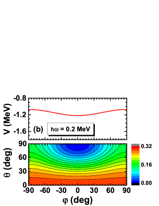
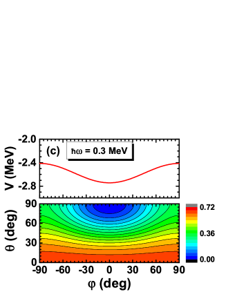
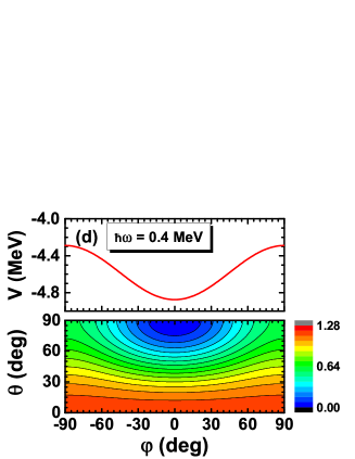
Figure 2: (Color online) Lower panels: Contour plots of total Routhian surface $E^{\prime}(\theta,\varphi)$ for a triaxial rigid body rotor with $\gamma=-30^{\circ}$ at the frequencies $\hbar\omega=0.1$, $0.2$, $0.3$ and $0.4~{}\rm MeV$. All energies at each rotational frequency are normalized with respect to the absolute minimum. Upper panels: The collective potential $V(\varphi)$ as a function of $\varphi$ extracted from the corresponding total Routhian surface calculation.

Minimizing the Routhian $E^{\prime}(\theta,\varphi)$ with $\theta$ for given $\varphi$, we find that the minimum along $\theta$ direction is always at $\theta=90^{\circ}$ for any value of $\varphi$ at each rotational frequency. The corresponding extracted collective potentials $V(\varphi)$ are shown in the upper panels of Fig. 2(a)-(d) respectively for $\hbar\omega=0.1$, $0.2$, $0.3$, and $0.4~{}\rm MeV$. Again, the potential energy is symmetrical about $\varphi=0^{\circ}$ in correspondence with the results displayed in the lower panels of Fig. 2(a)-(d). For all cases, the potential $V(\varphi)$ is a harmonic oscillator type that has only one minimum at $\varphi=0^{\circ}$, corresponding to the rotation about 1-axis. The stiffness of the collective potential becomes larger as the rotational frequency increases. This is directly reflected by the increase of energy difference between $\varphi=\pm 90^{\circ}$ and $\varphi=0^{\circ}$. For example, the value is only $\sim 30~{}\rm keV$ at $\hbar\omega=0.1~{}\rm MeV$ while reaches to $\sim 600~{}\rm keV$ at $\hbar\omega=0.4~{}\rm MeV$.

IV.1.2 Collective levels and wave functions

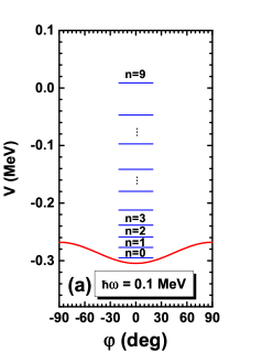
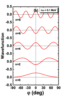
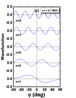
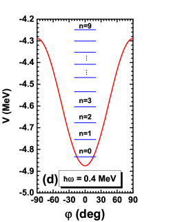
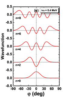
Figure 3: (Color online) The collective levels and wave functions obtained from the collective Hamiltonian. Upper panel: The ten lowest energy levels labeled as $n=0$-$9$ (left) and the corresponding wave functions for even-$n$ (middle) and odd-$n$ (right) states at the frequency $\hbar\omega=0.1~{}\rm MeV$. Lower panel: The ten lowest energy levels labeled as $n=0$-$9$ (left) and the corresponding wave functions for even-$n$ (middle) and odd-$n$ (right) states at the frequency $\hbar\omega=0.4~{}\rm MeV$.

The collective potential obtained above and the mass parameter obtained using Eq. (15) are combined to construct the collective Hamiltonian for investigating the simple wobbling motion. Diagonalizing the collective Hamiltonian, the collective energy levels and wave functions at each cranking frequency are yielded. Taking $\hbar\omega=0.1~{}\rm MeV$ and $0.4~{}\rm MeV$ for example, the obtained ten lowest wobbling energy levels and corresponding wave functions are presented Fig. 3. It is obviously seen that the wave functions are symmetric for even-$n$ levels and antisymmetric for odd-$n$ levels with respect to $\varphi\to-\varphi$ transformation. Thus the broken signature symmetry in the TAC model is restored in the collective Hamiltonian by the quantization of wobbling angle $\varphi$ and the consideration of quantum fluctuation along $\varphi$ motion. In addition, it is also shown that the wave function of the most favored wobbling energy levels are symmetric.

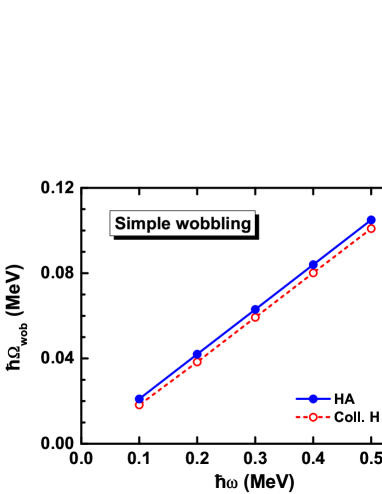
Figure 4: (Color online) The simple wobbling frequency $\hbar\Omega_{\rm wob}$ obtained by collective Hamiltonian in comparison with those of HA formula (II.3).

The wobbling frequency $\hbar\Omega_{\rm wob}$ defined as the energy difference between the lowest two levels for a certain rotational frequency in the collective Hamiltonian is shown in Fig. 4 in comparison with those from HA formula (II.3). It is seen that both collective Hamiltonian and HA give the linear increasing trend of wobbling frequency with respect to rotational frequency. For the HA results, this is just the expected since the coefficient $\sqrt{\frac{(\mathcal{J}_{1}-\mathcal{J}_{2})(\mathcal{J}_{1}-\mathcal{J}_{3})}{\mathcal{J}_{3}\mathcal{J}_{2}}}$ in the HA formula (II.3) is a positive constant values. For the collective Hamiltonian results, this can be also readily understood according to the stiffness of the collective potential, as shown in the upper panels of Fig. 2(a)-(d), which becomes larger with increasing of rotational frequency. The wobbling frequency given by HA formula is a bit larger than that by collective Hamiltonian results from the fact that the simple harmonic approximation for the collective potential would overestimate the stiffness of the potential, as shown in Fig. 5.

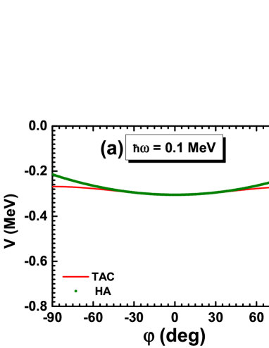
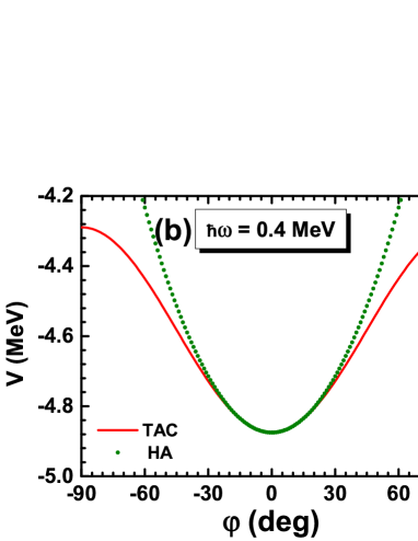
Figure 5: (Color online) The collective potentials obtained by HA (12) in comparison with those by TAC (11) at frequencies $\hbar\omega=0.1$ and $0.4~{}\rm MeV$.

IV.1.3 Comparison with TRM solutions

The simple wobbler solutions discussed here can be exactly obtained by TRM. To study the accuracy of collective Hamiltonian scheme, in Fig. 6, the energies of the four lowest wobbling bands $n=1,2,3,4$ relative to the $n=0$ yrast sequence obtained by collective Hamiltonian are displayed in comparison with those from TRM and HA. In the TRM, the states possesses $D_{2}$ symmetry so that the spectrum is restricted to the states with $(-1)^{n}=(-1)^{I}$ Bohr and Mottelson (1975), i.e., only even spins for even-$n$ wobbling bands while only odd appear for odd-$n$ wobbling bands. The even-$n$ wobbling bands are more energetically favored than odd-($n+1$) wobbling bands. Hence, the wobbling energies are calculated in different ways for even-$n$ and odd-$n$ wobbling bands. For even-$n$ wobbling bands, the wobbling energies are directly calculated as the energy difference with respect to $n=0$ wobbling bands $E_{\rm wob}^{n}=E_{n}(I)-E_{0}(I)$, while for odd-$n$ wobbling bands calculated as the energy difference with respect to the interpolated energies by $n=0$ wobbling band $E_{\rm wob}^{n}(I)=E_{n}(I)-[E_{0}(I+1)+E_{0}(I-1)]/2$. The spin in the TRM is treated as a good quantum number, while in the collective Hamiltonian it is not but a expectation value of angular momentum operator on the rotational state with given rotational frequency.

It is observed from Fig. 6 the increasing trend of wobbling energies with spin for each wobbling bands. With the increasing of $n$, the HA results gradually deviate from TRM, which indicates that the wobbling motion gradually deviates from harmonic oscillation character. The collective Hamiltonian excellently reproduce the TRM results even for the large-$n$ wobbling bands. The collective Hamiltonian based on TAC approach, however, provides a new perspective to interpret the variation trend of wobbling frequency with spin by exploring the variation trend of stiffness of the collective potential.

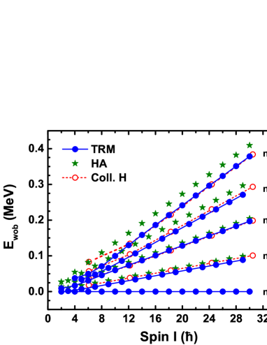
Figure 6: (Color online) Energy spectra of four simple wobbling bands $n=1,2,3,4$ relative to the $n=0$ yrast sequence obtained by collective Hamiltonian in comparison with TRM and HA. In the TRM, the wobbling energies for even-$n$ wobbling bands are calculated as $E_{\rm wob}^{n}=E_{n}(I)-E_{0}(I)$, while for odd-$n$ wobbling bands $E_{\rm wob}^{n}(I)=E_{n}(I)-[E_{0}(I+1)+E_{0}(I-1)]/2$.

IV.2 Longitudinal wobbler

Now we discuss the longitudinal wobbler, where a $h_{11/2}$ proton particle is assumed to couple to a triaxial rotor and its angular momentum is parallel to the axis with the largest moment of inertia. The rigid body type of moments of inertia (III) are used here too.

IV.2.1 Collective potential

In the contour plots of Fig. 7(a)-(d), the total Routhians for longitudinal wobbling motions obtained TAC are shown at the rotational frequencies $\hbar\omega=0.1$, $0.2$, $0.3$, and $0.4~{}\rm MeV$. Similar to the case of simple wobbling, the total Routhian is also symmetrical with respect to the $\varphi=0^{\circ}$ line and the minima always locate at $(\theta=90^{\circ},\varphi=0^{\circ})$ regardless of how fast the nucleus rotates. This is very clear since both the proton particle and triaxial rotor angular momenta in the longitudinal wobbling system are oriented along the short axis, the axis with the largest moment of inertia.

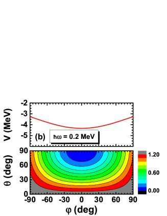
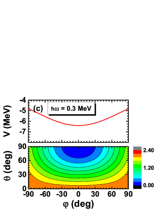
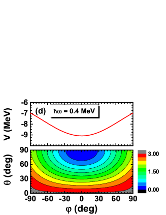
Figure 7: (Color online) Same as Fig. 2 but for longitudinal wobbling motion, where a proton $h_{11/2}$ particle coupled to a triaxial rigid body rotor with $\gamma=-30^{\circ}$.

With the total Routhian, the extracted collective potentials $V(\varphi)$ are presented at $\hbar\omega=0.1$, $0.2$, $0.3$, and $0.4~{}\rm MeV$ in the upper panels of Fig. 7(a)-(d). It is clearly seen that the collective potentials presented here are very similar as those presented in the upper panels of Fig. 2(a)-(d) for simple wobbling motions, while the only difference is that the stiffness here become larger. Therefore, similar discussions for simple wobbling motion still hold true here. It is worth to stress that the deeper potentials here are attributed to the proton particle and its contribution would become larger at larger rotational frequency. For example, at $\hbar\omega=0.1~{}\rm MeV$, the energy difference between $\varphi=\pm 90^{\circ}$ and $\varphi=0^{\circ}$ is $\sim 540~{}\rm keV$ and reaches to $\sim 2080~{}\rm keV$ at $\hbar\omega=0.4~{}\rm MeV$. Comparing with the simple wobbling motions, one obtains the contribution from proton increases from $\sim 510~{}\rm keV$ at $\hbar\omega=0.1~{}\rm MeV$ to $1480~{}\rm keV$ at $0.4~{}\rm MeV$.

IV.2.2 Mass parameter

The mass parameter for longitudinal wobbling motion is calculated by Eq. (19) and shown in Fig. 8. As discussed in Sec. II, since the effective moments of inertia for 1-axis decreases with the rotational frequency, the mass parameter increases with increasing rotational frequency. This increasing characteristic is different from the simple wobbler, where the mass parameter is constant at any rotational frequency.

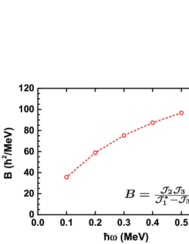
Figure 8: (Color online) The calculated mass parameter as a function of rotational frequency $\hbar\omega$ for longitudinal wobbling motion.

IV.2.3 Collective levels and wave functions

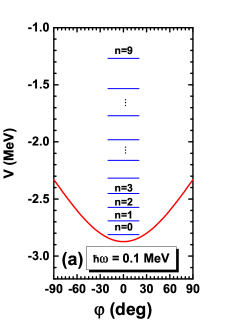
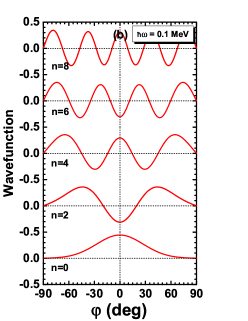
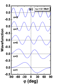
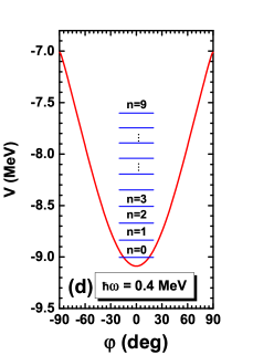
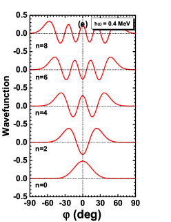
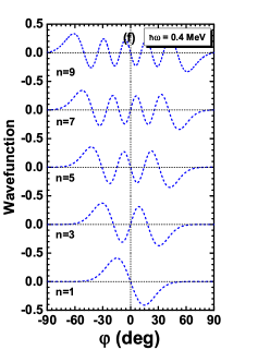
Figure 9: (Color online) Same as Fig. 3 but for longitudinal wobbling motion.

The obtained collective energy levels and corresponding wave functions are illustrated in Fig. 9 for $\hbar\omega=0.1$ and $0.4~{}\rm MeV$. Again, the wave functions presented here are similar as those presented in Fig. 3 for simple wobbling motions.

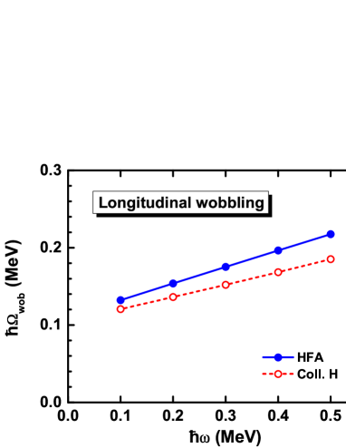
Figure 10: (Color online) The longitudinal wobbling frequency $\hbar\Omega_{\rm wob}$ obtained by collective Hamiltonian in comparison with those of HFA approximation (II.3).

In Fig. 10, the obtained wobbling frequency calculated by the collective Hamiltonian, is in comparison with the results obtained by HFA approximation (II.3). It is found that both collective Hamiltonian and HFA give the increased wobbling frequency as function of rotational frequency. However, the HFA results are larger than the collective Hamiltonian ones over the whole range of rotational frequency. To understand the origin of the differences between HFA and collective Hamiltonian, the collective potential obtained by HFA approximation in comparison with the results obtained by TAC at $\hbar\omega=0.1~{}\rm MeV$ and $\hbar\omega=0.4~{}\rm MeV$ are shown in Fig. 11. It is seen that the stiffness of collective potential calculated by HFA are larger than the collective Hamiltonian at both $\hbar\omega=0.1$ and $0.4~{}\rm MeV$. Since the mass parameter in the collective Hamiltonian is the same as the in the HFA, the wobbling frequency of HFA is larger than collective Hamiltonian. Besides the harmonic approximation as for simple wobbling motion, the HFA further introduces that the proton particle rigidly aligns its angular momentum along short axis. Hence it deviates larger from the collective Hamiltonian for the longitudinal wobbling motion ($\sim 20~{}\rm keV$, see Fig. 10) than HA for the simple wobbling motion ($\sim 5~{}\rm keV$, see Fig. 4).

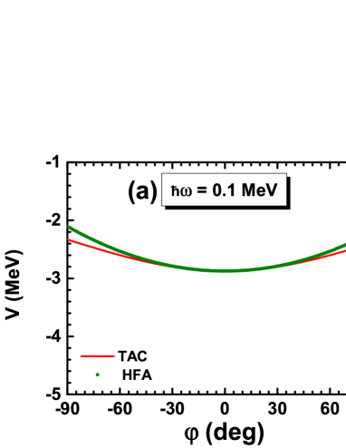
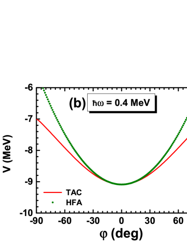
Figure 11: (Color online) The collective potentials obtained by HFA (18) in comparison with those by TAC (17) at frequencies $\hbar\omega=0.1$ and $0.4~{}\rm MeV$.

IV.2.4 Comparison with PRM solutions

The exact solutions for longitudinal wobbling motion can be obtained by PRM. In order to investigate the quality of the collective Hamiltonian, the energies of the two lowest wobbling bands $n=1,2$ relative to the $n=0$ yrast sequence obtained by collective Hamiltonian are shown in Fig. 12 in comparison with those from PRM. In PRM, for odd-$n$, the wobbling energies are calculated as $E_{\rm wob}^{n}=E_{n}(I)-E_{0}(I)$, while for even-$n$ wobbling bands are calculated as $E_{\rm wob}^{n}(I)=E_{n}(I)-[E_{0}(I+1)+E_{0}(I-1)]/2$. It is found that the collective Hamiltonian can reproduce the PRM very well. With the increasing spin, the wobbling energy increases. The results calculated by HFA are also shown in Fig. 12. The wobbling energies given by HFA are larger than those obtained by both PRM and collective Hamiltonian.

Both HFA and collective Hamiltonian are approximate solutions with respect to PRM. In the HFA approximation, the harmonic oscillator potential and the frozen alignment of proton particle are assumed. In the collective Hamiltonian, however, only the mass parameter is calculated with the HFA approximation, while the collective potential is calculated by TAC model without prior assuming the frozen alignment with respect to any axis for proton particle. The PRM exactly diagonals the particle rotor coupling Hamiltonian and thus gives the exact solutions. From this point of view, the collective Hamiltonian has improved the descriptions for the collective potential and provides a more accurate solution than HFA.

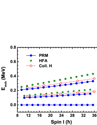
Figure 12: (Color online) Energy spectra of two longitudinal wobbling bands $n=1,2$ relative to the $n=0$ yrast sequence obtained by collective Hamiltonian in comparison with PRM and HFA. In the PRM, the wobbling energies for even-$n$, the wobbling energies are calculated as $E_{\rm wob}^{n}=E_{n}(I)-E_{0}(I)$, while for odd-$n$ $E_{\rm wob}^{n}(I)=E_{n}(I)-[E_{0}(I+1)+E_{0}(I-1)]/2$.

IV.3 Transverse wobbler

For transverse wobbling motions, the proton particle angular momentum is supposed to be perpendicular to the axis with the largest moment of inertia. In the present investigation, the irrotational flow type of moments of inertia (III) is employed to satisfy this requirement.

IV.3.1 Collective potential

The total Routhians calculated by TAC for a $h_{11/2}$ proton particle coupled to a triaxial irrotational flow rotor with $\gamma=-30^{\circ}$ in the $(\theta,\varphi)$ plane are displayed at the rotational frequencies $\hbar\omega=0.1$, $0.2$, $0.3$, $0.4~{}\rm MeV$ in contour plots of Fig. 13(a)-(d). The potential energy surfaces are also symmetric with the $\varphi=0^{\circ}$ line. In contrast to the simple and longitudinal wobbling motions, the minima in the potential energy surfaces change from $\varphi=0^{\circ}$ to $\varphi\neq 0^{\circ}$ with the increasing frequency. As discussed in Ref. Frauendorf and Dönau (2014), this implies the axis of uniform rotation is tilted from $s$ axis into the $s$-$i$ plane.

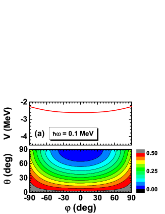
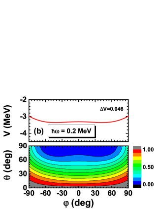
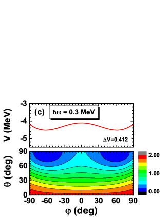
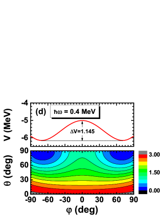
Figure 13: (Color online) Same as Fig. 2 but for transverse wobbling, where a proton $h_{11/2}$ particle coupled to a triaxial irrotational flow rotor with $\gamma=-30^{\circ}$.

The extracted collective potentials $V(\varphi)$ for transverse wobbling motion are shown in the upper panels of Fig. 13(a)-(d). For $\hbar\omega=0.1~{}\rm MeV$, the potential $V(\varphi)$ is a harmonic oscillator type which has only one minimum at $\varphi=0^{\circ}$, which corresponds to the uniform rotation around 1-axis. For $\hbar\omega\geq 0.20~{}\rm MeV$, the potential $V(\varphi)$ has two symmetrical minima, which corresponds to the tilted rotation. Due to the appearance of the potential barrier, the tilted solutions are achieved in the body-fixed frame. The heights of barrier defined as $\Delta V=V(0)-V_{\rm min}$ (in MeV) with $V_{\rm min}$ being the value of the potential at the minimum presented also in the figure. It is found that the potential barrier increases with the rotational frequency, e.g., from $0.046~{}\rm MeV$ at $\hbar\omega=0.20~{}\rm MeV$ to $1.145~{}\rm MeV$ at $\hbar\omega=0.40~{}\rm MeV$.

IV.3.2 Mass parameter

The obtained mass parameter calculated by Eq. (19) as a function of rotational frequency is shown in Fig. 14. Since here the irrotational flow type of moments of inertia (III) with $\gamma=-30^{\circ}$ assumed, i.e., $\mathcal{J}_{1}=\mathcal{J}_{3}$, the deduced mass parameter is linear dependence on rotational frequency. The mass parameter (19) is derived based on the assumption of harmonic frozen alignment approximation, therefore, it is strictly speaking valid only at the wobbling motion region and will becomes invalid in the tilted rotation region. Nevertheless, as a rough approximation, the mass parameter formula (19) is used for the calculations over the whole range of rotational frequency.

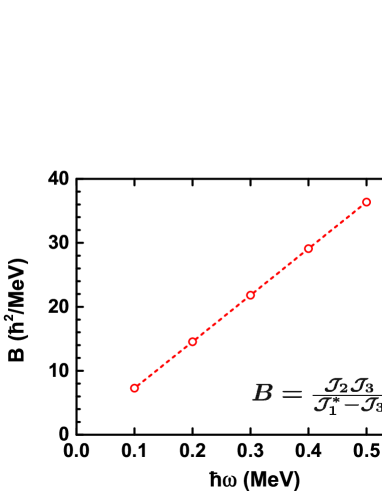
Figure 14: (Color online) Same as Fig. 8 but for transverse wobbling motion.

IV.3.3 Collective levels and wave functions

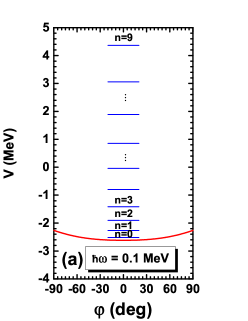
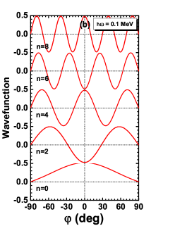
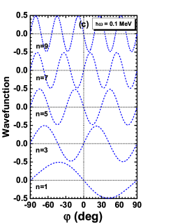
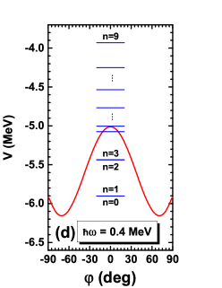
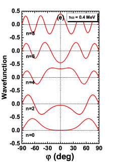
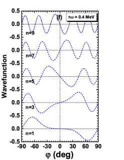
Figure 15: (Color online) Same as Fig. 3 but for transverse wobbling motion.

The obtained collective levels and wave functions are shown in Fig. 15 for $\hbar\omega=0.1$, $0.4~{}\rm MeV$. Similar as the simple and longitudinal wobbling motions, the wave functions are symmetric for even-$n$ levels and antisymmetric for odd-$n$ levels. For $n=0$, the peak of the wave function locates around $\varphi=0^{\circ}$ at $\hbar\omega=0.1~{}\rm MeV$, while moves towards to $\varphi=90^{\circ}$ at $\hbar\omega=0.4~{}\rm MeV$. In addition, when the rotational frequency increases, the probability distributions determined by the absolute square of wave functions tend to show similar pattern for $n=0$ and $n=1$ levels. This is consistent with that their energy differences, as shown in left panel of Fig. 15, tend to zero.

The calculated wobbling frequencies are shown in Fig. 16. It can be seen from Fig. 16, the wobbling frequency decreases with the rotational frequency. This decreasing is attributed to the increase of the potential barrier, as shown in the upper panels of Fig. 13, which will suppress the tunneling probability between the two symmetrical TAC solutions. At $\hbar\omega\geq 0.3~{}\rm MeV$, the wobbling frequency tends to zero, which implies the transverse wobbling motion is terminated. For comparison, the wobbling frequencies calculated by HFA are also shown in Fig. 16. The decreasing trend is clearly observed. As discussed above, at the critical rotational frequency $\hbar\omega_{\rm c}=j_{\pi}/(\mathcal{J}_{2}-\mathcal{J}_{1})\approx 0.183~{}\rm MeV$ the wobbling frequency becomes zero and above it the HFA formula becomes invalid. Comparing with the collective Hamiltonian, HFA gives about $50~{}\rm keV$ smaller values of wobbling frequency. It is also worthy to mention that the HFA gives a more rapid decreasing trend than the collective Hamiltonian since the quantum fluctuations are not taken into account in the HFA beyond the region of transverse wobbling motion.

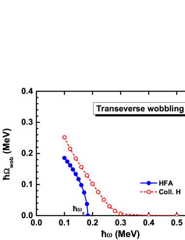
Figure 16: (Color online) Same as Fig. 10 but for transverse wobbling motion.

IV.3.4 Comparison with PRM solutions

In Fig. 17, the energies of the two lowest wobbling bands $n=1,2$ relative to the $n=0$ yrast sequence obtained by collective Hamiltonian are shown in comparison with the PRM solutions and HFA results. It is found that the collective Hamiltonian can reproduce the PRM results well at the region of wobbling motions. For $I\geq 16.5\hbar$, the wobbling energies of $n=1$ increase in the PRM, which indicates the onset of transitions from the transverse to longitudinal wobbling motions as discussed in Ref. Frauendorf and Dönau (2014). This transition, however, is not reproduced by the present collective Hamiltonian since the boundary conditions of wave functions at $\varphi=\pm 90^{\circ}$ are assumed to be zero. Further investigation on this topic will be done in the future.

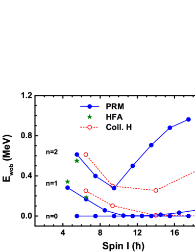
Figure 17: (Color online) Same as Fig. 12 but for transverse wobbling motion.

V Summary

In summary, three types of wobble modes for the nucleus have been studied in the framework of collective Hamiltonian. The simple wobbler is a pure triaxial rotor assumed with rigid body type of moments of inertia. With an odd $h_{11/2}$ proton of particle character coupling to the triaxial rotor, the longitudinal wobbler is achieved by arranging the moments of inertia as rigid body type, while the transverse wobbler achieved as irrotational body type. The collective potential in the collective Hamiltonian are calculated based on TAC approach. The mass parameter are obtained by HA for simple wobbling motion, while by HFA approximation for longitudinal and transverse wobbling motions.

Diagonalizing the collective Hamiltonian, the energies and the wave functions of the wobbling states are yielded. The obtained wobbling energies of simple wobbler are compared with the results calculated by HA and TRM, while those of longitudinal and transverse wobblers energies are compared with HFA and PRM. It is found that the results of collective Hamiltonian are in good agreement with those exact solutions by TRM or PRM.

In accord with those obtained by HA or HFA formula Frauendorf and Dönau (2014), it is observed that the wobbling frequency increases with the rotational frequency for the simple and longitudinal wobbling motions, while decreases for the transverse wobbling motion. It is presented here that these variation trends of the wobbling frequency are in association with the stiffness of the collective potentials. It should be mentioned that the present work has provided a new way to understand the wobbling phenomena, which in particular may further contribute to the investigation of nuclear wobbling based on a realistic TAC theory such as tilted axis cranking density functional theory Meng et al. (2013).

References

- Bohr and Mottelson (1975) A. Bohr and B. R. Mottelson, Nuclear structure, vol. II (Benjamin, New York, 1975).
- Bengtsson et al. (1984) R. Bengtsson, H. Frisk, F. May, and J. Pinston, Nucl. Phys. A 415, 189 (1984).
- Hamamoto and Sagawa (1988) I. Hamamoto and H. Sagawa, Phys. Lett. B 201, 415 (1988).
- Frauendorf and Meng (1997) S. Frauendorf and J. Meng, Nucl. Phys. A 617, 131 (1997).
- Frauendorf (2001) S. Frauendorf, Rev. Mod. Phys. 73, 463 (2001).
- Meng and Zhang (2010) J. Meng and S. Q. Zhang, J. Phys. G: Nucl. Part. Phys. 37, 064025 (2010).
- Frauendorf and Dönau (2014) S. Frauendorf and F. Dönau, Phys. Rev. C 89, 014322 (2014).
- Ødegård et al. (2001) S. W. Ødegård, G. B. Hagemann, D. R. Jensen, M. Bergström, B. Herskind, G. Sletten, S. Törmänen, J. N. Wilson, P. O. Tjøm, I. Hamamoto, et al., Phys. Rev. Lett. 86, 5866 (2001).
- Jensen et al. (2002a) D. R. Jensen, G. B. Hagemann, I. Hamamoto, S. W. Ødegård, B. Herskind, G. Sletten, J. N. Wilson, K. Spohr, H. Hübel, P. Bringel, et al., Phys. Rev. Lett. 89, 142503 (2002a).
- Jensen et al. (2002b) D. R. Jensen, G. B. Hagemann, I. Hamamoto, S. W. Ødegård, M. Bergstrom, B. Herskind, G. Sletten, S. Tormanen, J. N. Wilson, P. O. Tjom, et al., Nucl. Phys. A 703, 3 (2002b).
- Schönwaßer et al. (2003) G. Schönwaßer, H. Hübel, G. B. Hagemann, P. Bednarczyk, G. Benzoni, A. Bracco, P. Bringel, R. Chapman, D. Curien, J. Domscheit, et al., Phys. Lett. B 552, 9 (2003).
- Bringel et al. (2005) P. Bringel, G. Hagemann, H. Hübel, A. Al-khatib, P. Bednarczyk, A. Bürger, D. Curien, G. Gangopadhyay, B. Herskind, D. Jensen, et al., Eur. Phys. J. A 24, 167 (2005).
- Amro et al. (2003) H. Amro, W. C. Ma, G. B. Hagemann, R. M. Diamond, J. Domscheit, P. Fallon, A. Gorgen, B. Herskind, H. Hubel, D. R. Jensen, et al., Phys. Lett. B 553, 197 (2003).
- Hagemann (2004) G. B. Hagemann, Eur. Phys. J. A 20, 183 (2004).
- Hartley et al. (2009) D. J. Hartley, R. V. F. Janssens, L. L. Riedinger, M. A. Riley, A. Aguilar, M. P. Carpenter, C. J. Chiara, P. Chowdhury, I. G. Darby, U. Garg, et al., Phys. Rev. C 80, 041304 (2009).
- Zhu et al. (2009) S. J. Zhu, Y. X. Luo, J. H. Hamilton, A. V. Ramayya, X. L. Che, Z. Jiang, J. K. Hwang, J. L. Wood, M. A. Stoyer, R. Donangelo, et al., Int. J. Mod. Phys. E 18, 1717 (2009).
- Hamamoto (2002) I. Hamamoto, Phys. Rev. C 65, 044305 (2002).
- Hamamoto and Mottelson (2003) I. Hamamoto and B. R. Mottelson, Phys. Rev. C 68, 034312 (2003).
- Tanabe and Sugawara-Tanabe (2006) K. Tanabe and K. Sugawara-Tanabe, Phys. Rev. C 73, 034305 (2006).
- Tanabe and Sugawara-Tanabe (2008) K. Tanabe and K. Sugawara-Tanabe, Phys. Rev. C 77, 064318 (2008).
- Shimizu and Matsuzaki (1995) Y. R. Shimizu and M. Matsuzaki, Nucl. Phys. A 588, 559 (1995).
- Matsuzaki et al. (2002) M. Matsuzaki, Y. R. Shimizu, and K. Matsuyanagi, Phys. Rev. C 65, 041303 (2002).
- Matsuzaki et al. (2003) M. Matsuzaki, Y. R. Shimizu, and K. Matsuyanagi, Eur. Phys. J. A 20, 189 (2003).
- Matsuzaki and Ohtsubo (2004) M. Matsuzaki and S. Ohtsubo, Phys. Rev. C 69, 064317 (2004).
- Matsuzaki et al. (2004) M. Matsuzaki, Y. R. Shimizu, and K. Matsuyanagi, Phys. Rev. C 69, 034325 (2004).
- Shimizu et al. (2005) Y. R. Shimizu, M. Matsuzaki, and K. Matsuyanagi, Phys. Rev. C 72, 014306 (2005).
- Shimizu et al. (2008) Y. R. Shimizu, T. Shoji, and M. Matsuzaki, Phys. Rev. C 77, 024319 (2008).
- Shoji and Shimizu (2009) T. Shoji and Y. R. Shimizu, Progr. Theor. Phys. 121, 319 (2009).
- Oi et al. (2000) M. Oi, A. Ansari, T. Horibata, and N. Onishi, Phys. Lett. B 480, 53 (2000).
- Chen et al. (2013) Q. B. Chen, S. Q. Zhang, P. W. Zhao, R. V. Jolos, and J. Meng, Phys. Rev. C 87, 024314 (2013).
- Mukhopadhyay et al. (2007) S. Mukhopadhyay, D. Almehed, U. Garg, S. Frauendorf, T. Li, P. V. M. Rao, X. Wang, S. S. Ghugre, M. P. Carpenter, S. Gros, et al., Phys. Rev. Lett. 99, 172501 (2007).
- Qi et al. (2009) B. Qi, S. Q. Zhang, J. Meng, S. Y. Wang, and S. Frauendorf, Phys. Lett. B 675, 175 (2009).
- Oi (2006) M. Oi, Phys. Lett. B 634, 30 (2006).
- Pauli (1933) W. Pauli, in Handbuch der Physik, vol. XXIV, p. 120 (Springer Verlag, Berlin, 1933).
- Ring and Schuck (1980) P. Ring and P. Schuck, The nuclear many body problem (Springer Verlag, Berlin, 1980).
- Meng et al. (2013) J. Meng, J. Peng, S. Q. Zhang, and P. W. Zhao, Front. Phys. 8, 55 (2013).