Optimal Spectrum Management in Two-User Interference Channels

Abstract

In this work, we address the problem of optimal spectrum management in continuous frequency domain in multiuser interference channels. The objective is to maximize the weighted sum of user capacities. Our main results are as follows: (i) For frequency-selective channels, we prove that in an optimal solution, each user uses maximum power; this result also generalizes to the cases where the objective is to maximize the weighted product (i.e., proportional fairness) of user capacities. (ii) For the special case of two users in flat channels, we solve the problem optimally.

I Introduction

In this paper, we address the problem of maximizing weighted sum of user capacities in multiuser communication systems in a common frequency band. We consider a continuous frequency domain. For frequency-selective channels, we prove that in an optimal solution, each user must use the maximum power available to it. This maximum-power result also holds in the case wherein the objective is to maximize the weighted product of user capacities; this objective is generally used to achieve proportional fairness. For the special case of two users in flat channels, we present an optimal spectrum management solution.

In a multiuser communication system [19, 10, 18], users either have to partition the available frequency (FDMA), or use frequency sharing (i.e., each user uses the entire spectrum), or a combination of the two (i.e., use partially-overlapping spectrums). Intuitively, FDMA is the optimal answer in the case of strong cross coupling (also referred to as strong interference scenario), and frequency sharing is optimal when the cross coupling is very weak. In the intermediate case, the optimal solution may be a combination of the two strategies [17] (i.e., users may use partially-overlapping spectrums).

There exist an extensive literature on the effect of cross coupling on choosing between FDMA and frequency sharing. The works in [6] and [11] provide sufficient conditions under which FDMA is guaranteed to be optimal; these conditions are group-wise conditions, i.e., each pair of users need to satisfy the condition. Recently, Zhao and Pottie [17] derived a tight condition which when satisfied by a pair of users guarantees that the given pair uses orthogonal frequencies (i.e, FDMA for the pair). Their result holds for any pareto optimal solution.

In the general interference scenarios in multiuser systems, the weighted sum-rate maximization problem is a non-convex optimization problem, and is generally hard to solve [15]. However, two general approaches have been proposed: (i) One approach considers the Lagrangian dual problem decomposed in frequency after first descretizing the spectrum [16]; the resulting Lagrangian dual problem is convex and potentially easier to solve [3, 12]. More importantly, [12] proves that the duality gap goes to zero when the number of “sub-channels” goes to infinity. However, the time-complexity of their method is a high-degree polynomial in the number of sub-channels (thus, becoming prohibitively expensive for the continuous frequency domain problem). (ii) The second approach changes the formulation of the problem to get an equivalent primal domain convex maximization problem [17]. Eventhough, the above approaches almost reduce the spectrum management problem to a convex optimization problem, they fall short of designing an optimal or approximation algorithm with bounded convergence.

The recent works in [17, 2] find the optimal solution for the special case of two “symmetric” users; their result is very specific, and doesn’t generalize to weighted or non-symmetric links. In another insightful work, [14] gives a characterization of the optimal solution for the two-user case which essentially yields a four to six variable equation. Our work essentially improves on these results and solves the problem for the general case of two users, using an entirely different technique.

Discrete Frequency Spectrum Management. In other related works, [12] and [13] consider the spectrum management problem in discrete frequency domain, wherein the available spectrum is already divided into given orthogonal channels and user power spectral densities are constant in each channel. Their motivation for considering the discrete version is to facilitate a numerical solution [12]. The discrete version is shown to be NP-hard (even for two users), and in [11] the authors give a sufficient condition for the optimal to be an FDMA solution. Even when restricted to FDMA solutions, they observe that the discrete version remains inapproximable, but provide a PTAS [13] for the continuous version (when restricted to FDMA solutions). Note that, for two users, the discrete version remains NP-hard [11], while the continuous version has been solved optimally in our paper (Section IV). Thus, discretizing the spectrum seems to make the spectrum allocation problem only harder, contrary to the motivation in [12]. Moreover, discretization of a given spectrum can actually reduce achievable capacity.

Our Results. In this paper, we address the following spectrum management problem: Given a spectrum band of width $W$ and a set of $n$ users each with a maximum transmit power, the SAPD (spectrum allocation and power distribution) problem is to determine power spectrum densities of the users in the continuous frequency domain to maximize the weighted sum of user capacities (as computed by the generalized Shannon-Hartley theorem). For the above SAPD problem, we present the following results.

• For frequency-selective channels, we show that in an optimal SAPD solution, each user must use the maximum transmit power. We extend the result to the cases wherein the objective is to maximize the weighted product of user capacities.

• For the special case of two users in flat channels, we design an optimal solution for the SAPD problem. This is a direct improvement of the recent recent in [17] which solves the problem optimally for the special case of two users with symmetric (equal channel gains and noise) and flat channels.

II Problem Formulation, and Notations

Model, Terms, and Notations. We are given a set of users $i$ (formed by a transmitter $s_{i}$ and a receiver $r_{i}$) and a frequency spectrum $[0,W]$. The background noise at the receiver of user $i$ is assumed to be white, i.e., constant across the spectrum, and has a constant value of $N_{i}$ (Watts/Hz) at each frequency. We use $h_{ij}(x)$ to denote channel gain between the sender of user $i$ and the receiver of user $j$ at frequency $x$.

Power Spectrum Density (PSD) $p_{i}(x)$; Total Power. For a user $i$, the power spectral density (PSD) is a function $p_{i}:[0,W]\mapsto\mathbb{R}_{\leq 0}$ that gives the power at each frequency of the signal used by the transmitter $s_{i}$ to communicate with its receiver $r_{i}$. Thus, $p_{i}(x)$ is the power of $s_{i}$’s signal at frequency $x$. In this paper, we allow arbitrary PSD functions. The total power used by a user $i$ is given by $\int\limits_{0}^{W}p_{i}(x)dx.$

Maximum Total Power. Each user $i$ is associated with a maximum total power $P_{i}$, which is the bound on the total power used by its transmitter $s_{i}$. That is, each PSD function $p_{i}(x)$ must satisfy the below condition:

$$\int\limits_{0}^{W}p_{i}(x)dx\leq P_{i}.$$ (1)

Spectrum Used. Given a PSD function $p_{i}(x)$ for a user $i$, the spectrum used by user $i$ is defined as $\{x|p_{i}(x)>0\}$, i.e., the set of frequencies wherein the power is non-zero. Thus, disjoint spectrums are orthogonal.

User Capacity. Given PSD functions $\{p_{i}(x)\}$ for a set of users in a communication system, the (maximum achievable rate) capacity $C_{i}$ of a user $i$ can be determined using the generalized Shannon-Hartly theorem as below. Here, we assume that the signals to be Gaussian processes, and treat interference as noise, as in prior works [12, 13, 11, 6].

$$C_{i}=\int\limits_{0}^{W}{\log\left(1+\frac{p_{i}(x)h_{ii}(x)}{I_{i}(x)+N_{i}}\right)dx}.$$ (2)

Above, $h_{ii}$ is the channel gain, and $I_{i}(x)$ is the total interference on frequency $x$ at the receiver $r_{i}$ due to other users. The interference $I_{i}(x)$ is computed as follows.

$$I_{i}(x)=\sum_{j\neq i}p_{j}(x)h_{ji}(x).$$

Spectrum Allocation and Power Distribution (SAPD) Problem. Given a set of users $\{1,2,\ldots,n\}$, maximum total power values $P_{i}$ for each user $i$, noise $N_{i}$ at each receiver $r_{i}$, and an available frequency spectrum $[0,W]$, the Spectrum Allocation and Power Distribution (SAPD) problem is to determine the PSD functions $\{p_{i}(x)\}$ for the given users such that the total (system) weighted capacity $\sum_{i}\omega_{i}C_{i}$ is maximized where $\omega_{i}$ are the given weights, under the constraint of Equation 1 (i.e., the total power used by each user $i$ is at most $P_{i}$). Note that determination of PSD functions also gives the allocation of spectrum across users (i.e., spectrums used by each user).

III Optimal SAPD Solution Uses Maximum Power

In this section, we prove that in an optimal SAPD solution, each user uses maximum total power. We note that our result does not contradict the prior “binary-power control” results of [4, 8, 7, 5] who consider a different and restricted model. In particular, they consider a model wherein each user uses a constant PSD across the available spectrum (i.e., each user either uses the entire spectrum with a constant PSD or remains silent). For this model, they show that to achieve maximum sum of user rates either (i) each user uses maximum power, or (ii) one of the users is silent (with the other user using maximum power). In contrast, in our model (wherein each user can use an arbitrary PSD function, and thus, an arbitrary subset of the spectrum), we show that each user must use maximum power to achieve maximum sum of user capacities. In fact, it is easy to see from our Lemma 2 that, in our model, the sum of rates achieved when one user is silent is always sub-optimal.

Theorem 1

For frequency-selective channels, in an optimal SAPD solution, each user uses maximum power, i.e., for each user $i$, $\int\limits_{0}^{W}p_{i}(x)dx=P_{i}$.

Proof:

Let $n$ be the number of users. Consider an optimal solution $\{p_{i}(x)\}$, where $p_{i}(x)$ is the PSD of the $i^{th}$ user. Assume that the claim of the theorem doesn’t hold, i.e., there is a user $k$ such that

$$p^{\prime}=P_{k}-\int_{0}^{W}{p_{k}(x)dx}>0.$$

Below, we use $p^{\prime}$ to improve on the given solution, which will contradict our assumption that the given solution is optimal and thus, proving the theorem.

Now, for an appropriate constant $\epsilon$ (as determined later), we change the given optimal solution as follows.

• First, in the spectrum $[0,\epsilon]$, we power-off all the users, i.e., for all $i$, we set $p_{i}(x)=0$ for $x\in[0,\epsilon]$.

• Second, we uniformly add the power $p^{\prime}$ to $k$’s PSD in the spectrum $[0,\epsilon]$, i.e., we set $p_{k}(x)$ to $p^{\prime}/\epsilon$ for $x\in[0,\epsilon]$.

The first change causes a decrease in the capacity of every user (including $k$), while the second change results in some new capacity for $k$. We can compute these amounts as follows.

• The decrease $\bigtriangledown_{i}$ in capacity of each user $i$ (including $k$) due to the changes can be computed as:

  $$\bigtriangledown_{i} = \int_{0}^{\epsilon}\log\left(1+\frac{p_{i}(x)h_{ii}(x)}{I_{i}(x)+N_{i}}\right)dx$$

  $$\leq \epsilon\log(1+\frac{p_{max}h_{max}}{N_{min}})$$ (3)

  Above, $N_{min}=\min_{i}N_{i}$, $p_{max}=\max_{i,x}p_{i}(x)$, and $h_{max}=\max_{i,x}h_{ii}(x)$, where $x\in[0,\epsilon]$ and $i$ varies over all users.

• The new capacity $C^{\prime}_{k}$ of user $k$ in $[0,\epsilon]$ after the second change is:

  $$C^{\prime}_{k} = \int_{0}^{\epsilon}\log\left(1+\frac{(p^{\prime}/\epsilon)h_{kk}(x)}{N_{k}}\right)dx$$ (4)

  $$\geq \epsilon\log(1+\frac{p^{\prime}h_{min}}{N_{k}\epsilon})$$

  Above, we have used $h_{min}=\min_{x}h_{kk}(x)$.

Now, the overall increase in the sum of weighted capacities of all the users is

$$\omega_{k}C^{\prime}_{k}-\sum_{i}\omega_{i}\bigtriangledown_{i}.$$

Below, we pick an $\epsilon$ that will ascertain $\omega_{k}C^{\prime}_{k}>\omega_{i}\sum_{i}\bigtriangledown_{i}$. Such an $\epsilon$ will imply that the above suggested changes result in an increase in the weighted sum of user capacities, and thus, proving the theorem. In particular, using Equation 3 and 4, we pick an $\epsilon$ such that:

$$\omega_{k}\epsilon\log(1+\frac{p^{\prime}h_{min}}{N_{k}\epsilon}) > \epsilon\sum_{i}\omega_{i}\log(1+\frac{p_{max}h_{max}}{N_{min}})$$

$$\log(1+\frac{p^{\prime}h_{min}}{N_{k}\epsilon}) > (\frac{\sum_{i}\omega_{i}}{\omega_{k}})\log(1+\frac{p_{max}h_{max}}{N_{min}})$$

$$1+\frac{p^{\prime}h_{min}}{N_{k}\epsilon} > (1+\frac{p_{max}h_{max}}{N_{min}})^{(\frac{\sum_{i}\omega_{i}}{\omega_{k}})}$$

$$\epsilon < \frac{p^{\prime}h_{min}}{N_{k}((1+\frac{p_{max}h_{max}}{N_{min}})^{(\frac{\sum_{i}\omega_{i}}{\omega_{k}})}-1)}.$$

Since the above expression is positive, there exists an $\epsilon$ for which the above suggested changes result in an increase in the weighted sum of user capacities. This contradicts the assumption that the original solution is optimal, and thus, proving the theorem. ∎

Theorem 1 can be easily generalized to the case wherein the objective is to maximize the weighted product of user capacities, i.e., to achieve proportional fairness. We defer the proof to Appendix A.

Theorem 2

For the SAPD problem wherein the objective is to maximize the weighted product of user capacities, the optimal solution uses maximum power for each user.  

IV Optimal SAPD Solution for Two Users in Flat Channels

In this section, we present an optimal solution for the SAPD problem for the special case of two users in flat channels. We use $h_{ij}$ to denote the channel gain, i.e., $h_{ij}(x)=h_{ij}$ for all $x$. For clarity of presentation, in this section, we implicitly assume the given weights $\omega_{i}$ to be uniform and unit; the generalization of our results to non-uniform weights is straightforward.

We start with an important lemma. The lemma’s proof is very tedious (see Appendix B).

Lemma 1

For a two user SAPD problem in flat channels, there exists an optimal solution wherein the PSD of each user is constant in the spectrum shared by the users. More formally, there exists an optimal solution such that if $S_{1}$ and $S_{2}$ are the spectrums used by the respective users, then for $x\in(S_{1}\cap\ S_{2})$, $p_{i}(x)=c_{i}$ for some constants $c_{i}$ ($i$ = 1,2).  

A somewhat related result from [6] states that any SAPD solution for $n$ users can be expressed using piecewise-constant PSD’s over appropriate 2$n$ pieces of the available spectrum; this result requires 4 pieces for $n=2$ users. In contrast, our above lemma implies a stronger result for an SAPD solution for two users, and is essential to our result.

Optimal SAPD Solution for Two Users. Consider a system with two users and an available spectrum $[0.W]$. The optimal SAPD solution can take three possible forms, viz., (i) the users use disjoint subspectrums, (ii) both users use the same subspectrum, (iii) the users use partially-overlapping (i.e., non-disjoint and non-equal) subspectrums. We can solve the first and the second cases optimally by using the below Lemmas 2 and 3 respectively. We defer the proofs to Appendix C, but Lemma 2 is a slight generalization of a result from [9] while Lemma 3 follows easily from Equation 2 and Lemma 1.

Lemma 2

Consider a system of two users $\{1,2\}$, and an available spectrum $[0,W]$. If the spectrums used by the two users are disjoint, then the maximum system capacity is

$$W\log(1+\frac{P_{1}h_{11}}{WN_{1}}+\frac{P_{2}h_{22}}{WN_{2}}),$$

and is achieved by dividing the spectrum in the ratio $N_{2}P_{1}h_{11}:N_{1}P_{2}h_{22}$.  

It is easy to see from the above lemma that the system capacity obtained when one of the users is silent is always less than that obtained by the partitioning the spectrum as suggested in the lemma.

Lemma 3

Consider a system with two users, and an available spectrum $[0,W]$. If the spectrums used by the two users is equal, then the maximum system capacity possible is:

$$W\log(1+\frac{P_{1}h_{11}}{P_{2}h_{21}+WN_{1}})+W\log(1+\frac{P_{2}h_{22}}{P_{1}h_{12}+WN_{2}}).$$

 

In the following paragraph, we show how to compute an optimal solution for the remaining third case, viz., wherein users use partially-overlapping subspectrums. The overall optimal SAPD solution can be then computed by taking the best of the optimal solutions for the above three cases.

Optimal Partially-Overlapping SAPD Solution. Consider an SAPD solution that is optimal among all partially-overlapping SAPD solutions. In such a solution, the available spectrum can be divided into three subspectrums $S_{1}$, $S_{2}$, and $S_{12}$, where $S_{1}$ and $S_{2}$ are used exclusively by user 1 and 2 respectively and $S_{12}$ is used by both the users. We assume $S_{1}$ and $S_{2}$ to be non-zero; the cases wherein one of them is zero are easier (see Appendix D. Now, since the noise is white, we can assume without loss of generality, that these three subspectrums are contiguous. It is easy to see that each user 1 must use a constant PSD in $S_{1}$, and user 2 must use a constant PSD in $S_{2}$. Also, by Lemma 1, we know that each user must use a constant PSD in $S_{12}$, and each of the three subspectrums. Finally, by Lemma 5 (see Appendix C), the PSD of user 1 in $S_{1}$ must be greater than its PSD in $S_{12}$; similarly, the PSD of user 2 in $S_{2}$ must be greater than its PSD in $S_{12}$. Now, let $\sigma_{1}$ and $\sigma_{2}$ be the PSD’s in $S_{12}$ of user $1$ and $2$ respectively, $\sigma_{1}+c_{1}$ be the PSD of user 1 in $S_{1}$, and $\sigma_{2}+c_{2}$ be the PSD of user $2$ in $S_{2}$. See Figure 1. The total system capacity can now be written as follows.

$$\begin{array}[]{ll}B\ =&S_{1}\log(1+\frac{(\sigma_{1}+c1)h_{11}}{N_{1}})+S_{2}\log(1+\frac{(\sigma_{2}+c_{2})h_{22}}{N_{2}})+\\ &S_{12}(\log(1+\frac{\sigma_{1}h_{11}}{\sigma_{2}+N_{1}})+\log(1+\frac{\sigma_{2}h_{22}}{\sigma_{1}+N_{2}}))\end{array}$$

To find the optimal SAPD solution of the above form, we need to essentially find values of the seven variables $S_{1},S_{2},S_{12},\sigma_{1},c_{1},\sigma_{2}$ and $c_{2}$ such that the above $B$ is maximized. We do so by determining six independent equations that must hold true for an optimal $B$. These six equations will help us eliminate all but one of the seven variables in $B$, yielding a formulation of $B$ in terms of a single variable. We can then differentiate $B$ with respect to the remaining variable, find the root of the differential equation equated to zero, and thus, determine the value of all the seven variables. Below, we derive the six equations (Equations 5 to 10) that relate the above seven variables. Below, $S_{1}$, $S_{2}$ and $S_{12}$ refer to the sizes of the corresponding spectrums.

• Since $W$ is the size of the total available spectrum, we have (by a simple application of Lemma 2):

  $$W=S_{1}+S_{2}+S_{12}$$ (5)

• Since $P_{1}$ and $P_{2}$ are the maximum total power of users $1$ and $2$ respectively, by Theorem 1, we have:

  $$P_{1} = S_{1}(\sigma_{1}+c_{1})+S_{12}\sigma_{1}$$ (6)

  $$P_{2} = S_{2}(\sigma_{2}+c_{2})+S_{12}\sigma_{2}$$ (7)

• Note that the PSD’s of the users 1 and 2 in $S_{1}$ and $S_{2}$ respectively should satisfy the values computed in Lemma 2, else the solution can be improved. Thus, we have:

  $$\frac{S_{1}}{S_{2}}=\frac{N_{2}P_{1}h_{11}}{N_{1}P_{2}h_{22}}$$ (8)

• Below, we show how to derive the remaining two equations, which require some tedious analysis.

Remaining Two Equations (Eqns 9-10). Let us now consider a small portion of the spectrum called $S$ — taken partly from $S_{1}$ and $S_{12}$. In an optimal solution, redistribution of power within $S$ should not lead to an improved total capacity. Without any loss of generality, let us assume $S$ to be of size $(w+1)$, with $w>0$ in the exclusive part ($S_{1}$) and $1$ in the shared part ($S_{3}$). See Figure 1. Thus, the total power used by the first user in $S$ is $w(c_{1}+\sigma_{1})+\sigma_{1}$. Let the optimal distribution of this total power for user 1 within $S$ be in the ratio of $k:(1-k)$ ($0\leq k\leq 1$) between the exclusive and shared parts of $S$. Now, the total capacity of both users in $S$ for the above power distribution is given by:

$$\begin{array}[]{ll}C(k)=&w\log(1+\frac{k(w(c_{1}+\sigma_{1})+\sigma_{1})h_{11}}{wN_{1}})+\\ &\log(1+\frac{(1-k)(w(c_{1}+\sigma_{1})+\sigma_{1})h_{11}}{\sigma_{2}h_{21}+N_{1}})+\\ &\log(1+\frac{\sigma_{2}h_{22}}{h_{12}(1-k)(w(c_{1}+\sigma_{1})+\sigma_{1})+N_{2}})\end{array}$$

Since $C(k)$ is connected and derivable for $0\leq k\leq 1$, $C(k)$ can be optimal only at $k$ = 0, 1, or when $\frac{dC}{dk}=0$. Having $k$ = 0 or 1 will contradict our choice of $S$; thus, $\frac{dC(k)}{dk}$ must be zero at optimal $C(k)$. Since we started with an optimal SAPD solution, where the capacity $C(k)$ must also be optimal, the value of $\frac{dC}{dk}$ must be zero for the $k=\frac{w(c_{1}+\sigma_{1})}{w(c_{1}+\sigma_{1})+\sigma_{1}}$ (based on the distribution of power in the original solution), and this must be true for any $w$ in $(0,x]$ where $x$ is the size of $S_{1}$ (the exclusive part of the spectrum).

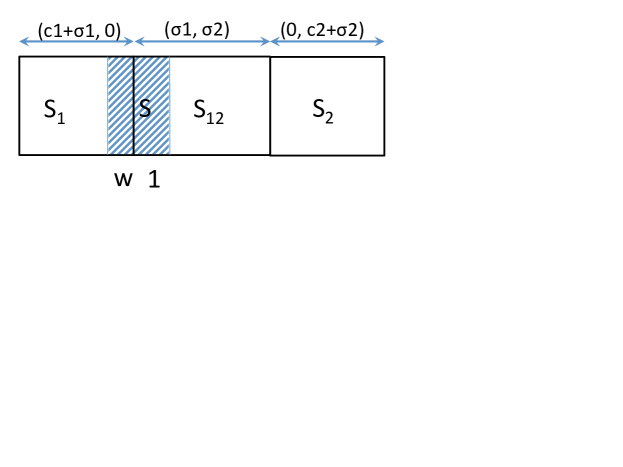
Figure 1: $S_{1}$ and $S_{2}$ are subspectrums used exclusively by users 1 and 2 respectively, and $S_{12}$ is the subspectrum used by both the users. The shaded part of the spectrum is $S$ (used to derive the final two equations) and is composed of two subspectrums of width 1 and $w$ respectively. The top of the figures denotes the PSDs used by the users, e.g., $(c1+\sigma_{1},0)$ signifies that the PSD values of the two users is $c1+\sigma_{1}$ and $0$ respectively in $S_{1}$.

Analyzing $dC(k)/dk$. We computed $\frac{dC(k)}{dk}$ at $k=\frac{w(c_{1}+\sigma_{1})}{w(c_{1}+\sigma_{1})+\sigma_{1}}$. After simplification, the numerator in the resulting expression can be written as $w(\sigma_{1}+c_{1})\Gamma_{1}+\sigma_{1}\Gamma_{1}$, where

$$\begin{array}[]{ll}\Gamma_{1}=&{h_{22}}N_{1}^{2}\sigma_{2}+2{h_{22}h_{11}}N_{1}\sigma_{1}\sigma_{2}+{h_{22}h_{11}}c_{1}N_{1}\sigma_{2}\\ &+\ {h_{22}}N_{1}\sigma_{2}^{2}-c_{1}N_{2}^{2}{h_{11}}^{2}+c_{1}{h_{11}h_{22}}\sigma_{2}^{2}\\ &-\ c_{1}{h_{22}}N_{2}{h_{11}}^{2}\sigma_{2}+2N_{2}{h_{11}}\sigma_{1}\sigma_{2}+{h_{22}}N_{2}{h_{11}}\sigma_{2}^{2}\\ &+\ {h_{22}h_{11}}^{2}\sigma_{1}^{2}\sigma_{2}-c_{1}{h_{11}}^{2}\sigma_{1}^{2}+{h_{11}}\sigma_{1}^{2}\sigma_{2}\\ &+\ 2{h_{22}h_{11}}\sigma_{1}\sigma_{2}^{2}+N_{2}^{2}{h_{11}}\sigma_{2}-2c_{1}N_{2}{h_{11}}^{2}\sigma_{1}\end{array}$$

Since the numerator of $\frac{dC(k)}{dk}$ should be zero regardless of $w$’s value in $(0,x]$, we must have that $\Gamma_{1}$ is zero. Similarly, for user 2, we must have $\Gamma_{2}=0$, where $\Gamma_{2}$ is similarly defined as $\Gamma_{1}$. Thus, we get the fifth and sixth equations as:

$$\Gamma_{1} = 0$$ (9)

$$\Gamma_{2} = 0$$ (10)

Eliminations of Variables. It is easy to verify that the derived six equations are independent, and hence, are sufficient to eliminate six (out of the total seven) variables as desired. However, the order of elimination needs to be chosen carefully chosen to avoid getting into a unsolvable polynomial of high degree. We choose the following order of elimination. From Equation 5, we get:

$$S_{12}=W-S_{1}-S_{2}$$

Substituting the above in Equation 6 and 7, and solving the resulting two equations for $S_{1}$ and $S_{2}$, we get

$$S_{1} = \frac{-W\sigma_{1}^{2}+P_{2}\sigma_{1}+P_{1}c_{2}-Wc_{2}\sigma_{2}}{c_{1}c_{2}-\sigma_{1}\sigma_{2}}$$

$$S_{2} = \frac{-W\sigma_{2}^{2}+P_{1}\sigma_{2}+P_{2}c_{1}-Wc_{1}\sigma_{1}}{c_{1}c_{2}-\sigma_{1}\sigma_{2}}$$

We can now write Equation 8 as follows.

$$\frac{\frac{-W\sigma_{1}^{2}+P_{2}\sigma_{1}+P_{1}c_{2}-Wc_{2}\sigma_{2}}{c_{1}c_{2}-\sigma_{1}\sigma_{2}}}{\frac{-W\sigma_{2}^{2}+P_{1}\sigma_{2}+P_{2}c_{1}-Wc_{1}\sigma_{1}}{c_{1}c_{2}-\sigma_{1}\sigma_{2}}}=\frac{N_{2}P_{1}h_{11}}{N_{1}P_{2}h_{22}}$$

In the above equation, we substitute $c_{1}$ and $c_{2}$ by the expressions derived from Equations 9 and 10 respectively. Note that Equations 9 and 10 are linear in $c_{1}$ and $c_{2}$ respectively, and hence, facilitating the above substitutions. After the above substitutions and tedious simplications, we actually get a fourth-degree equation in $\sigma_{1}$ (in terms of $\sigma_{2}$). Since four-degree equations have closed-form solutions, we solve the resulting equation to express $\sigma_{1}$ in terms of $\sigma_{2}$. The resulting expressions are extremely long and tedious, and hence omitted here (see [1] for details). The above allows us to express $B$ solely in terms of $\sigma_{2}$. Thus, the single-variable equation $dB/d(\sigma_{2})=0$ can be solved efficiently using well-known numerical methods, since $dB/d(\sigma_{2})$ is connected and derivable in $\sigma_{2}$ with bounded derivatives, and $\sigma_{2}$ has a bounded range (see Appendix E). Finally, as $B$ is continuous and bounded, we can then use the roots of $dB/d(\sigma_{2})=0$ to compute the optimal $B$.

Note on Multiple Roots. Note that some of the intermediate equations in the above described process may not be linear, and hence may yield multiple roots. That only results in multiple expressions for $B$ (in terms of $\sigma_{2}$), and hence, multiple possible sets (but, at most 16 sets) of parameter values. We compute the total system capacity $B$ for each of these set of values, and pick the one that yields the largest value of $B$.

V Conclusions

In this paper, we have considered the spectrum management problem in multiuser communication systems. We proved that in an optimal solution, each user uses the maximum power. For the special case of two users in flat channels, we solve the problem optimally. Our future work is focussed on generalization of our techniques to communication systems with more than two users.

Appendix A Proof of Theorem 2

Proof of Theorem 2. We make the same changes as suggested in Theorem 1’s proof. The suggested changes will result in the objective value changing from

$$(\Pi_{i}w_{i}C_{i})\ {\rm to}\ w_{k}(C_{k}+C^{\prime}_{k}-\bigtriangledown_{k})\Pi_{i\neq k}w_{k}(C_{i}-\bigtriangledown_{i}),$$

where $w_{i}$ and $C_{i}$ are the weights and total capacity of user $i$. Note that $(C_{k}-\bigtriangledown_{k})\geq 0.$ Let $\eta^{\prime}$ be the ratio of the above objective values (new to old value). Below, we show that there exists an $\epsilon$ that makes $\eta^{\prime}>1$. This would imply that the given optimal solution is suboptimal (a contradiction), and thus, proving the theorem.

Now, using Eqn 3 and 4, we get:

$$\eta^{\prime} \triangleq \left(\prod_{i\neq k}{\frac{C_{i}-\bigtriangledown_{i}}{C_{i}}}\right){\frac{C_{k}+(C^{\prime}_{k}-\bigtriangledown_{k})}{C_{k}}}$$

$$\geq \left(\prod_{i\neq k}{\frac{C_{min}-\bigtriangledown_{i}}{C_{min}}}\right){\frac{C_{max}+(C^{\prime}_{k}-\bigtriangledown_{k})}{C_{max}}}$$

$$\geq \left(\frac{C_{min}-\bigtriangledown_{max}}{C_{min}}\right)^{n-1}{\frac{C_{max}+(C^{\prime}_{k}-\bigtriangledown_{k})}{C_{max}}}$$

$$\geq (1-a_{1}\epsilon)^{n-1}(1+a_{2}\epsilon\log(1+\frac{a_{3}}{\epsilon})-a_{4}\epsilon)$$

where $a_{1},a_{2},a_{3},a_{4}$ are appropriate positive constants (independent of $\epsilon$) and $\bigtriangledown_{max}$ is the expression in Equation 3. Let $\eta$ denote the last expression above. We can now state the following:

$$\begin{array}[t]{ll}(i)&\lim_{\epsilon\to 0}\eta=1.\\ (ii)&\begin{array}[t]{rl}\frac{d\eta}{d\epsilon}=&(1-a_{1}{\epsilon})^{n-1}\times\\ &\Bigg{(}\frac{-a_{1}(n-1)\left(1+a_{2}\epsilon\log(1+a_{3}/\epsilon)-a_{4}\epsilon\right)}{1-a_{1}{\epsilon}}+\\ &a_{2}\log(1+a_{3}/\epsilon)-\frac{a_{2}\epsilon}{(1+a_{3}/\epsilon)\epsilon^{2}}-a_{4}\Bigg{)}\\ =&(1-a_{1}{\epsilon})^{n-1}.\xi\\ \end{array}\end{array}$$

Also, one can easily verify that $\lim_{\epsilon\to 0^{+}}\xi=+\infty$ and $(1-a_{1}{\epsilon})^{n-1}$ is always positive. Thus, $\frac{d\eta}{d\epsilon}$ is positive when $\epsilon\to 0^{+}$, which implies (from (i) above) that there exists an $\epsilon>0$ such that $\eta>1$ and thus $\eta^{\prime}>1$.  

Appendix B Proof of Lemma 1

Proof of Lemma 1. Instead of directly proving Lemma 1, we prove the following lemma.

Lemma 4

Consider two users 1 and 2, and an SAPD solution (not necessarily optimal) $\{p_{1}(x),p_{2}(x)\}$ where each user uses the entire available spectrum $[0,W]$. We claim that there always exists an SAPD solution $\{p^{\prime}_{1}(x),p^{\prime}_{2}(x)\}$ with equal or higher total capacity such that either (i) both the PSD functions $p^{\prime}_{i}(x)$ are constant in $[0,W]$, or (ii) one of the users does not use the entire spectrum $[0,W]$.  

Lemma 1 can be easily inferred from Lemma 4 by using contradiction. Lets consider an SAPD problem instance for two users, which has no optimal solution wherein the PSDs of the two users is constant in the shared part of the spectrum. From the set of optimal solutions, lets pick the one with minimum size of the shared spectrum. According to lemma 4, we can find another solution with equal or higher capacity in which either the size of the shared spectrum is reduced or the users use constant PSD’s in the shared spectrum. In either case, we get a contradiction. We now present the proof of Lemma 4.

Proof of Lemma 4. We start with defining a couple of notations.

$k$-rectangular SAPD Solution. An SAPD solution $\{p_{1}(x),p_{2}(x)\}$ is considered to be $k$-rectangular if there exists frequency values $w_{i}$, such that $0=w_{0}<w_{1}<w_{2}<\ldots<w_{k-1}<w_{k}=W$ such that for each $j$ ($1\leq j\leq k$) and $x$ ($w_{j-1}\leq x<w_{j}$), we have $p_{1}(x)=c_{1j}$ and $p_{2}(x)=c_{2j}$ for some constants $c_{1j}$ and $c_{2j}$.

2-rectangular SAPD Solution. First, we prove the lemma for the special case when the given SAPD solution $\{p_{1}(x),p_{2}(x)\}$ is $2$-rectangular. Without loss of generality, let us assume that the given SAPD solution is the optimal $2$-rectangular SAPD solution, under the given total powers (viz., $\int_{0}^{W}p_{1}(x)dx$ and $\int_{0}^{W}p_{2}(x)dx$ respectively). Now, we can write the given optimal $2$-rectangular SAPD solution as follows.

• For $0\leq x<w$, $p_{1}(x)=\sigma_{1}$, $p_{2}(x)=\sigma_{2}$.

• For $w\leq x<W$, $p_{1}(x)=\sigma_{1}+\Delta_{1}$, $p_{2}(x)=\sigma_{2}+\Delta_{2}$.

Above, $\sigma_{i}>0$, $\Delta_{i}+\sigma_{i}>0$, for each $i$. Let $\Psi_{1}$ and $\Psi_{2}$ be the aggregate (sum over two links) capacity per unit-bandwidth in the two sub-spectrums $[0,w]$ and $(w,W]$ respectively. Without loss of generality, let us assume $\Psi_{1}\leq\Psi_{2}$. We consider the following four cases.

$\Psi_{1}=\Psi_{2}=\Psi$ and $\Delta_{1}\Delta_{2}=0$. In this case, the given solution can be easily converted to a 1-rectangular solution of equal or higher capacity.

$\Psi_{1}=\Psi_{2}=\Psi$ and $\Delta_{1}\Delta_{2}>0$. Without loss of generality, we assume $\Delta_{2}\geq\Delta_{1}>0$. Note that, in either sub-spectrum, if we “scale-up” the PSD value of each link, then the aggregate capacity (per unit-bandwidth) would increase. Thus, for any $a>1$, the PSD value of $a.\sigma_{1}$ and $a.\sigma_{2}$ would result in a higher aggregate capacity than $\Psi_{1}$ (= $\Psi_{2})$. Now, since $\Delta_{i}>0$, there exists $a>1$ such that $a.\sigma_{i}<\sigma_{i}+\Delta_{i}$ for each $i$. For such an $a$, changing the PSD value in the second sub-spectrum from $\sigma_{i}+\Delta_{i}$ to $a\sigma_{i}$ results in an increase in the aggregate capacity (with lower total power). Thus, the given solution is not an optimal 2-rectangular solution. QED.

$\Psi_{1}=\Psi_{2}=\Psi$ and $\Delta_{1}\Delta_{2}<0$. Without loss of generality, we can assume $\Delta_{1}>0$ and $\Delta_{2}<0$. Now, if $W>2w$, let $[g_{1},g_{2}]=[0,2w]$ otherwise let $[g_{1},g_{2}]=[W-2w,W]$. Let $X(b)$ and $Y(b)$ be such that $\log X(b)$ and $\log Y(b)$ are the capacities per unit-bandwidth of the first and second links when they use a constant PSD value of $\sigma{1}+b\Delta{1}$ and $\sigma{2}+b\Delta{2}$ respectively; here, $b\in[-\frac{\sigma{1}}{\Delta_{1}},-\frac{\sigma{2}}{\Delta{2}}]\supseteq[0,1]$. Below, we show how to choose appropriate $b$ values to create a better 2-rectangular solution, or an equal-capacity solution wherein one of the links does not use the entire spectrum.

Let $X_{max}$ be the maximum value of $X(b)$ over the above range of $b$. Since the above function $X(b)$ is reversible, we can define the function $f=Y(X^{-1}):[0,X_{max}]\mapsto\mathbb{R}_{\geq 0}$ such that $f(x)$ gives the capacity-per-bandwidth of the second link when the capacity/bandwidth of the first link is $x$ due to constant PSD values of $\sigma{1}+b\Delta{1}$ and $\sigma{2}+b\Delta{2}$ respectively for some $b$; note that, $b$ is unique for a given $x$. We can show (we omit the details here) that the second-derivative of the function ($d(df(x)/dx)/dx$) cannot be zero in $[0,X_{max}]$. Thus, the function $f(x)$ has no inflection point in the range $[0,X_{max}]$, and hence, we can plot the various possibilities for the $f(x)$ relative to $y=2^{\Psi}/x$ as shown in Figure 2. Note that $f(x)$ is maximum at $x=1$, and is 1 at $X_{max}$, and intersects the $y=2^{\Psi}/x$ plot at two $x$ values corresponding to $b=0$ and $b=1$ (since $\Psi_{1}=\Psi_{2}=\Psi$). Moreover, since $X(b)$ is monotonically increasing in $b$, we get the values/ranges of $b$ as depicted in the figure. Now, for each of the four possibilities of $f(x)$ depicted in the Figure 2, we can prove the lemma as follows.

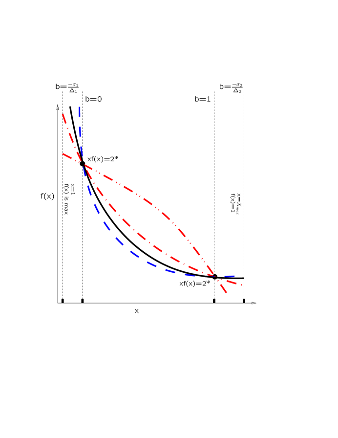
Figure 2: Red and blue (dotted) curves are the possible shapes of $f(x)$; here, the black (solid) curve is $y=2^{\Psi}/x$.

• If $f(x)$ is one of the two red plots, then we pick $b=1/2$. For $b=1/2$, we get $X(b)Y(b)>2^{\Psi}$ and hence $\log X(b)+\log Y(b)>\Psi$. Now, if we can choose constant PSD values of $\sigma{1}+b\Delta{1}$ and $\sigma{2}+b\Delta{2}$ for the two links respectively in $[g_{1},g_{2}]$, we get a 2-rectangular solution in $[0,W]$ of higher total capacity within the given power constraint. QED.

• If $f(x)$ is the blue or the black plot, then we choose two values of $b$, viz., $b_{l}$ and $b_{r}$, so as to use PSD values of $\sigma_{i}+b_{l}\Delta_{i}$ in $[g_{1},w]$ and $\sigma_{i}+b_{r}\Delta_{i}$ in $[w,g_{2}]$ for each link $i$. For our purposes, we need to choose $b_{l}$ and $b_{r}$ such that they satisfy the following three conditions: (i) $-\sigma_{1}/\Delta_{1}\leq b_{l}\leq 0$, and $1\leq b_{r}\leq-\sigma_{2}/\Delta_{2}$ (to ensure that $b$ is in the valid range and the capacity/bandwidth is at least $\Psi$ in each sub-spectrum), and (ii) $b_{l}+b_{r}=1$ (to ensure that the total power used is at most the total power in the original solution, for each link), and (iii) $\sigma_{i}+b_{l}\Delta_{i}$ or $\sigma_{i}+b_{r}\Delta_{i}$ is zero for some $i$ (so that one of the links uses zero power in one of the sub-spectrums). To satisfy the above three conditions, we choose the pair $(b_{l},b_{r})$ as $(-\sigma_{1}/\Delta_{1},1+\sigma_{1}/\Delta_{1})$ if $1+\sigma_{1}/\Delta_{1}<-\sigma_{2}/\Delta_{2}$, or $(1+\sigma_{2}/\Delta_{2},-\sigma_{2}/\Delta_{2})$ otherwise. The above yields an SAPD solution of higher capacity wherein one of the links doesn’t use the entire spectrum. QED.

$\Psi_{1}<\Psi_{2}$. In this case, we consider sub-spectrums $[g_{1},w]$ and $[w,g_{2}]$ for some appropriate $g_{1}$ and $g_{2}$ (determined later), and increase the aggregate capacity within these sub-spectrums by appropriate redistribution of power.

Let $r=(g_{2}-w)/(w-g_{1})$, the ratio of the two sub-subspectrums, and $\tau=(g_{2}-g_{1})$. Let $P^{\prime}_{1}$ and $P^{\prime}_{2}$ be the total power used by link $1$ and $2$ in $[g_{1},g_{2}]$, i.e., $P^{\prime}_{i}={\tau}(\sigma_{i}+\Delta_{i}r/(r+1))$. Let $\Phi(r)$ be the aggregate capacity per bandwidth in $[g_{1},g_{2}]$ when the PSD values are $P^{\prime}_{1}/\tau$ and $P^{\prime}_{2}/\tau$ respectively for the two links. We now show that a “large-enough” $r$ will ensure that $(1+r)\Psi(r)>\Psi_{1}+r\Psi_{2}$, which will imply that in $[g_{1},g_{2}]$ the 1-rectangular solution yields a higher total capacity than the given solution. Observe the following: (i) $\lim_{r\rightarrow 0^{+}}{\Phi(r)=\Psi_{1}}$, (ii) $\lim_{r\rightarrow\infty}{\Phi(r)=\Psi_{2}}$, and (iii) $\phi(r)$ is connected. Since $\lim_{r\rightarrow\infty^{+}}{(1+r)\Phi(r)=(1+r)\Psi_{2}>\Psi_{1}+r\Psi_{2}}$, there exists a large-enough $r$ for which $(1+r)\Psi(r)>\Psi_{1}+r\Psi_{2}$. Once we find the appropriate $r$, we can determine $g_{1}$ and $g_{2}$ as follows: If $(r+1)w<W$, then pick $[g_{1},g_{2}]=[0,(r+1)w]$, else pick $[g_{1},g_{2}]=[w-(W-w)/r,W]$. Then, in $[g_{1},g_{2}]$, we use power-signals of $\sigma_{i}+\Delta_{i}r/(r+1)$ for link $i$, yielding a 2-rectangular solution with a higher-capacity than the given solution. QED.

$k$-rectangular Solution. This can be easily proven by induction on $k$, using the above result on $k=2$ as the base case.

Arbitrary SAPD Solution. Let $p_{1}(x)$ and $p_{2}(x)$ be the power-distribution functions for the given solution, and let $P^{*}_{i}=\int_{0}^{W}p_{i}(x)dx$ be the total powers used by the links. Assume that there is no solution of equal or higher capacity, in which one of the link doesn’t use the full spectrum. Let us construct an $n$-rectangular solution that “approximates” the given solution as follows: First, we divide the spectrum $[0,W]$ into $n$ equi-sized sub-spectrums, and then, within each sub-spectrum we use a constant PSD value of minimum $p_{i}(x)$ in that sub-spectrum. Note that the total power used by the link $i$ in the above $n$-rectangular solution is atmost $P^{*}_{i}$. Let $F_{n}$ be the total capacity of the above $n$-rectangular solution, and let $R$ be the total capacity of the 1-rectangular solution that uses a constant PSD of $P_{i}/W$ for each link. Since the lemma holds for $k$-rectangular solutions, we get that $F_{n}\leq R$ for any $n$. Now, if $C$ is the total capacity of the given solution, then by definition $C=\lim_{n\rightarrow+\infty}F_{n}$. Thus, we get $C\leq R$, which completes the proof.  

Appendix C Proofs of Lemma 2 and 5

Proof of Lemma 2. First, it is easy to see that the union of the disjoint spectrums must be the entire available spectrum. Let the links use disjoint spectrums of size $yW$ and $(1-y)W$ where $0\leq y\leq 1$. Since both links should use maximum power for maximum capacity, we can compute the total capacity as follows.

$$C=yW\log(1+\frac{P_{1}h_{11}}{yWN_{1}})+W(1-y)\log(1+\frac{P_{2}h_{22}}{(1-y)WN_{2}})$$

We can find the optimal value of $y$ by solving for $dC/dy=0$. We have:

$$\begin{array}[]{ll}\frac{dC(y)}{dy}=&W\big{(}\log(1+\frac{P_{1}h_{11}}{yWN_{1}})-\log(1+\frac{P_{2}h_{22}}{(1-y)WN_{2}})-\\ &\frac{P_{1}h_{11}}{yWN_{1}(1+\frac{P_{1}h_{11}}{yWN_{1}})}+\frac{P_{2}h_{22}}{(1-y)WN_{2}(1+\frac{P_{2}h_{22}}{(1-y)WN_{2}})}\big{)}\end{array}$$

The root of the equation $dC/dy=0$ is:

$$y=\frac{N_{2}P_{1}h_{11}}{N_{1}P_{2}h_{22}+N_{2}P_{1}h_{11}}.$$

Hence, the PSD’s of link $1$ and $2$ are $\frac{N_{1}P_{2}h_{22}+N_{2}P_{1}h_{11}}{WN_{2}h_{11}}$ and $\frac{N_{1}P_{2}h_{22}+N_{2}P_{1}h_{11}}{WN_{1}h_{22}}$ respectively and the optimal value of $C$ is:

$$C=W\log(1+\frac{P_{1}h_{11}}{WN_{1}}+\frac{P_{2}h_{22}}{WN_{2}})$$

 

Lemma 5.

Lemma 5

Consider a communication system with a single user 1, and an available spectrum $[0,W]$. Let the interference (from other users) in the sub-spectrums $[0,w]$ and $(w,W]$ be constant and equal to $I$ and $I^{\prime}$ respectively. If $I>I^{\prime}$, then to achieve maximum capacity for user 1, its PSD value in $[0,w]$ should be lower than in $(w,W]$.

Proof:

It is easy to see that for optimal capacity: (i) the PSD should be constant in each of the sub-spectrums, and (ii) the link should use maximum power. Now, if we divide the total power of $P_{1}$ into the two sub-spectrums in the ratio of $k:(1-k)$, for some $0\leq k\leq 1$, we get link capacity as:

$$C(k)=w\log(1+\frac{kP_{1}h_{11}}{w(I+N_{1})})+(W-w)\log(1+\frac{(1-k)P_{1}h_{11}}{(W-w)(I^{\prime}+N_{1})})$$

By solving $dC/dk=0$, we get $k=\frac{w}{W}+\frac{w}{WP_{1}h_{11}}(I^{\prime}-I)(W-w)$ which give us the PSD values of $\frac{1}{W}(P_{1}+(W-w)(I^{\prime}-I)/h_{11})$ and $\frac{1}{W}(P_{1}+w(I-I^{\prime})/h_{11})$ in the two sub-spectrums. This proves the lemma, since the first PSD value is always greater than the second PSD value. ∎

Appendix D Cases for $S_{1}$ or $S_{2}$ = 0.

Case where $S_{1}$ or $S_{2}$ is of Zero Size. Let $S_{1}=0$ and $S_{2}>0$. In this case, Equations 8 and 9 are not valid. At the same time, the variables $S_{1}$ and $c_{1}$ are eliminated from the system, and hence, we have two fewer equations and variables which only simplifies the problem. We can use the exact same order of elimination and technique to yield an optimal solution for this case. This case of $S_{2}=0$ and $S_{1}>0$ is similarly handled, and the case of $S_{2}=0$ and $S_{1}=1$ is already handled by Lemma 3.

Appendix E Upper Bound of $\sigma_{2}$

Upper bound of $\sigma_{2}$. Here, we show that there exists an upper bound for $\sigma_{2}$. Since the PSD’s used by users 1 and 2 in $S_{1}$ and $S_{2}$ is $(c_{1}+\sigma_{1})S_{1}$ and $(c_{2}+\sigma_{2})S_{2}$ respectively, we have the following (by applying Lemma 2, and using the PSD values computed therein):

$$c_{1}+\sigma_{1}=\frac{N_{2}(c_{1}+\sigma_{1})S_{1}h_{11}+N_{1}(c_{2}+\sigma_{2})S_{2}h_{22}}{(S_{1}+S_{2})N_{2}h_{11}},$$

$$c_{2}+\sigma_{2}=\frac{N_{2}(c_{1}+\sigma_{1})S_{1}h_{11}+N_{1}(c_{2}+\sigma_{2})S_{2}h_{22}}{(S_{1}+S_{2})N_{1}h_{22}},$$

and $c_{2}+\sigma_{2}=(c_{1}+\sigma_{1})\frac{N_{2}h_{11}}{N_{1}h_{22}}$. Let $\varsigma=\frac{N_{2}h_{11}}{N_{1}h_{22}}$ and $\gamma=\max(\varsigma,1)$. Let $P=P_{1}+P_{2}$, and recall that $c_{1},c_{2},\sigma_{1}$, and $\sigma_{2}$ are positive numbers. Thus, we have:

$$P = (c_{1}+\sigma_{1})S_{1}+(c_{2}+\sigma_{2})S_{2}+(\sigma_{1}+\sigma_{2})S_{12}$$

$$P > \frac{1}{\varsigma}(c_{2}+\sigma_{2})S_{1}+\sigma_{2}S_{2}+\sigma_{2}S_{12}$$

$$\gamma P > (\gamma/\varsigma)\sigma_{2}S_{1}+\gamma\sigma_{2}(S_{2}+S_{12})$$

$$\gamma P > \sigma_{2}(S_{1}+S_{2}+S_{12})\ \ \ (\rm{as}\ \gamma\geq 1,\varsigma)$$

$$\gamma P/W > \sigma_{2}$$

Thus, $\gamma P/W$ is an upper bound on $\sigma_{2}$, where $\gamma=\max(1,\frac{N_{2}h_{11}}{N_{1}h_{22}})$.

References

- [1] Matlab source codes for omitted mathematical details. http://tinyurl.com/b6yhdal.
- [2] S. R. Bhaskaran, Stephen V. Hanly, Nasreen Badruddin, and Jamie S. Evans. Maximizing the sum rate in symmetric networks of interfering links. IEEE Trans. on Information Theory, 2010.
- [3] R. Cendrillon, W. Yu, M. Moonen, J. Verlinden, and T. Bostoen. Optimal multiuser spectrum balancing for digital subscriber lines. Communications, IEEE Transactions on, 54(5):922–933, 2006.
- [4] M. Charafeddine and A. Paulraj. Maximum sum rates via analysis of 2-user interference channel achievable rates region. In IEEE CISS, 2009.
- [5] M. Ebrahimi, M. A. Maddah-ali, and A. K. Khandani. Power allocation and asymptotic achievable sum-rates in single-hop wireless networks. In IEEE CISS, 2006.
- [6] R. H. Etkin, A. Parekh, and D. Tse. Spectrum sharing for unlicensed bands. IEEE JSAC, 25(3), 2007.
- [7] A. Gjendemsj, D. Gesbert, G. E. Oien, and S. G. Kiani. Binary power control for sum rate maximization over multiple interfering links. IEEE Trans. Wireless Communications, 7(8), 2008.
- [8] A. Gjendemsjo, D. Gesbert, G.E. Oien, and S.G. Kiani. Optimal power allocation and scheduling for two-cell capacity maximization. In Intl. Symp. on Modeling and Optimization in Mobile, Ad Hoc and Wireless Networks, 2006.
- [9] R. Gummadi, R. Patra, H. Balakrishnan, and E. Brewer. Interference avoidance and control. In ACM HotNets, 2008.
- [10] Himanshu Gupta and P Sadayappan. Communication efficient matrix multiplication on hypercubes. In Proceedings of the sixth annual ACM symposium on Parallel algorithms and architectures, pages 320–329. ACM, 1994.
- [11] S. Hayashi and Z.-Q. Luo. Spectrum management for interference-limited multiuser communication systems. IEEE Trans. Inf. Theor., 2009.
- [12] Z.-Q. Luo and S. Zhang. Dynamic spectrum management: Complexity and duality. IEEE J. of Selected Topics in Signal Processing, 2008.
- [13] Z.-Q. Luo and S. Zhang. Duality gap estimation and polynomial time approximation for optimal spectrum management. ACM Trans. Sig. Proc., 2009.
- [14] H. Shen, Hang Zhou, R.A. Berry, and M.L. Honig. Optimal spectrum allocation in gaussian interference networks. In Asilomar Conf. on Signals, Systems and Computers, 2008.
- [15] W. Yu, G. Ginis, and J.M. Cioffi. Distributed multiuser power control for digital subscriber lines. IEEE JSAC, 2002.
- [16] W. Yu and R. Lui. Dual methods for nonconvex spectrum optimization of multicarrier systems. IEEE Trans. on Comm., 2006.
- [17] Y. Zhao and G.J. Pottie. Optimal spectrum management in multiuser interference channels. In ISIT, 2009.
- [18] Xianjin Zhu, Himanshu Gupta, and Bin Tang. Join of multiple data streams in sensor networks. IEEE Transactions on knowledge and Data Engineering, 21(12):1722–1736, 2009.
- [19] Xianjin Zhu, Bin Tang, and Himanshu Gupta. Delay efficient data gathering in sensor networks. In International Conference on Mobile Ad-Hoc and Sensor Networks, pages 380–389. Springer, 2005.