Intermittent Control in Man and Machine

Abstract

Intermittent control has a long history in the physiological literature and there is strong experimental evidence that some human control systems are intermittent. Intermittent control has also appeared in various forms in the engineering literature. This article discusses a particular mathematical model of Event-driven Intermittent Control which brings together engineering and physiological insights and builds on and extends previous work in this area. Illustrative examples of the properties of Intermittent Control in a physiological context are given together with suggestions for future research directions in both physiology and engineering.

1 Introduction

Conventional sampled-data control uses a zero-order hold, which produces a piecewise-constant control signal (Franklin et al., 1994), and can be used to give a sampled-data implementation which approximates a previously-designed continuous-time controller. In contrast to conventional sampled data control, intermittent control (Gawthrop and Wang, 2007), explicitly embeds the underlying continuous-time closed-loop system in a generalised hold. A number of version of the generalised hold are available; this chapter focuses on the system-matched hold (Gawthrop and Wang, 2011) which expicitly generates an open-loop intersample control trajectory based on the underlying continuous-time closed-loop control system. Other versions of the generalised hold include Laguerre function based holds (Gawthrop and Wang, 2007) and a “tapping” hold (Gawthrop and Gollee, 2012).

There are at three areas where intermittent control has been used:

1. continuous-time model-based predictive control where the intermittency is associated with on-line optimisation (Ronco et al., 1999; Gawthrop and Wang, 2009a, 2010),

2. event-driven control systems where the intersample interval is time varying and determined by the event times (Gawthrop and Wang, 2009b, 2011),

3. and physiological control systems which, in some cases, have an event-driven intermittent character (Loram and Lakie, 2002; Gawthrop et al., 2011). This intermittency may be due to the “computation” in the central nervous system. Although this Chapter is orientated towards physiological control systems, but we believe that it is more widely applicable.

Intermittent control has a long history in the physiological literature including (Craik, 1947a, b; Vince, 1948; Navas and Stark, 1968; Neilson et al., 1988; Miall et al., 1993a; Bhushan and Shadmehr, 1999; Loram and Lakie, 2002; Loram et al., 2011; Gawthrop et al., 2011). There is strong experimental evidence that some human control systems are intermittent (Craik, 1947a; Vince, 1948; Navas and Stark, 1968; Bottaro et al., 2005; Loram et al., 2012; van de Kamp et al., 2013b) and it has been suggested that this intermittency arises in the central nervous system (CNS) (van de Kamp et al., 2013a). For this reason, computational models of intermittent control are important and, as discussed below, a number of versions with various characteristics have appeared in the literature. Intermittent control has also appeared in various forms in the engineering literature including (Ronco et al., 1999; Zhivoglyadov and Middleton, 2003; Montestruque and Antsaklis, 2003; Insperger, 2006; Astrom, 2008; Gawthrop and Wang, 2007, 2009b; Gawthrop et al., 2012).

Intermittent control action may be initiated at regular intervals determined by a clock, or at irregular intervals determined by events; an event is typically triggered by an error signal crossing a threshold. Clock-driven control is discussed by Neilson et al. (1988) and Gawthrop and Wang (2007) and analysed in the frequency domain by Gawthrop (2009). Event-driven control is used by Bottaro et al. (2005, 2008), Astrom (2008), Asai et al. (2009), Gawthrop and Wang (2009b) and Kowalczyk et al. (2012). Gawthrop et al. (2011, Section 4) discuss event-driven control but with a lower limit $\Delta_{min}$ on the time interval between events; this gives a range of behaviours including continuous, timed and event-driven control. Thus, for example, threshold based event-driven control becomes effectively clock driven with interval $\Delta_{min}$ if the threshold is small compared to errors caused by relatively large disturbances. There is evidence that human control systems are, in fact, event driven (Navas and Stark, 1968; Loram et al., 2012; van de Kamp et al., 2013a; Loram et al., 2014). For this reason, this Chapter focuses on event-driven control.

As mentioned previously, intermittent control is based on an underlying continuous-time design method; in particular the classical state-space approach is the basis of the intermittent control of Gawthrop et al. (2011). There are two relevant versions of this approach: state feedback and output feedback. State-feedback control requires that the current system state (for example angular position and velocity of an inverted pendulum) is available for feedback. In contrast, output feedback requires a measurement of the system output (for example angular position of an inverted pendulum). The classical approach to output feedback in a state-space context (Kwakernaak and Sivan, 1972; Goodwin et al., 2001) is to use an observer (or the optimal version, a Kalman filter) to deduce the state from the system output.

Human control systems are associated with time-delays. In engineering terms, it is well-known that a predictor can be used to overcome time delay (Smith, 1959; Kleinman, 1969; Gawthrop, 1982). As discussed by many authors (Kleinman et al., 1970; Baron et al., 1970; McRuer, 1980; Miall et al., 1993b; Wolpert et al., 1998; Bhushan and Shadmehr, 1999; Van Der Kooij et al., 2001; Gawthrop et al., 2008, 2009, 2011; Loram et al., 2012), it is plausible that physiological control systems have built in model-based prediction. Following Gawthrop et al. (2011) this chapter bases intermittent controller on an underlying predictive design.

The use of networked control systems leads to the “sampling period jitter problem” (Sala, 2007) where uncertainties in transmission time lead to unpredictable non-uniform sampling and stability issues (Cloosterman et al., 2009). A number of authors have suggested that performance may be improved by replacing the standard zero-order hold by a generalised hold (Sala, 2005, 2007) or using a dynamical model of the system between samples (Zhivoglyadov and Middleton, 2003; Montestruque and Antsaklis, 2003). Similarly, event-driven control (Heemels et al., 2008; Astrom, 2008), where sampling is determined by events rather than a clock, also leads to unpredictable non-uniform sampling. Hence strategies for event-driven control would be expected to be similar to strategies for networked control. One particular form of event-driven control where events correspond to the system state moving beyond a fixed boundary has been called Lebesgue sampling in contrast to the so-called Riemann sampling of fixed-interval sampling (Astrom and Bernhardsson, 2002, 2003). In particular, Astrom (2008) uses a “control signal generator”: essentially a dynamical model of the system between samples as advocated by Zhivoglyadov and Middleton (2003) for the networked control case.

As discussed previously, intermittent control has an interpretation which contains a generalised hold (Gawthrop and Wang, 2007). One particular form of hold is based on the closed-loop system dynamics of an underlying continuous control design: this will be called the System-Matched Hold (SMH) in this Chapter. Insofar as this special case of intermittent control uses a dynamical model of the controlled system to generate the (open-loop) control between sample intervals, it is related to the strategies of both Zhivoglyadov and Middleton (2003) and Astrom (2008). However, as shown in this Chapter, intermittent control provides a framework within which to analyse and design a range of control systems with unpredictable non-uniform sampling possibly arising from an event-driven design. In particular, it is shown by Gawthrop and Wang (2011) that the SMH-based intermittent controller is associated with a separation principle similar to that of the underlying continuous-time controller, which states that the closed-loop poles of the intermittent control system consist of the control system poles and the observer system poles, and the interpolation using the system matched hold does not lead to the changes of closed-loop poles. As discussed by Gawthrop and Wang (2011), this separation principle is only valid when using the SMH. For example, intermittent control based on the standard zero-order hold (ZOH) does not lead to such a separation principle and therefore closed-loop stability is compromised when the sample interval is not fixed.

Human movement is characterised by low-dimensional goals achieved using high-dimensional muscle input (Shadmehr and Wise, 2005); in control system terms the system has redundant actuators. As pointed out by Latash (2012), the abundance of actuators is an advantage rather than a problem. One approach to redundancy is by using the concept of synergies (Neilson and Neilson, 2005): groups of muscles which act in concert to give a desired action. It has been shown that such synergies arise naturally in the context of optimal control (Todorov, 2004; Todorov and Jordan, 2002) and experimental work has verified the existence of synergies in vivo (Ting, 2007; Safavynia and Ting, 2012). Synergies may be arranged in hierarchies. For example, in the context of posture, there is a natural three-level hierarchy with increasing dimension comprising task space, joint space and muscle space. Thus, for example, a balanced posture could be a task requirement achievable by a range of possible joint torques each of which in turn corresponds to a range of possible muscle activation. This chapter focuses on the task space – joint space hierarchy previously examined in the context of robotics (Khatib, 1987).

In a similar way, humans have an abundance of measurements available; in control system terms the system has redundant sensors. As discussed by Van Der Kooij et al. (1999) and Van Der Kooij et al. (2001), such sensors are utilised with appropriate sensor integration. In control system terms, sensor redundancy can be incorporated into state-space control using observers or Kalman-Bucy filters (Kwakernaak and Sivan, 1972; Goodwin et al., 2001); this is the dual of the optimal control problem. Again sensors can be arranged in a hierarchical fashion. Hence optimal control and filtering provides the basis for a continuous-time control system that simultaneously applies sensor fusion to utilise sensor redundancy and optimal control to utilise actuator redundancy.

For these reasons, this Chapter extends the single-input single-output intermittent controller of Gawthrop et al. (2011) to the multivariable case. As the formulation of Gawthrop et al. (2011) is set in the state-space, this extension is quite straightforward. Crucially, the generalised hold, and in particular the system matched hold (SMH), remains as the heart of multivariable intermittent control.

The particular mathematical model of intermittent control proposed by Gawthrop et al. (2011) combines event-driven control action based on estimates of the controlled system state (position, velocity etc.) obtained using a standard continuous-time state observer with continuous measurement of the system outputs. This model of intermittent control can be summarised as “continuous attention with intermittent action”. However, the state estimate is only used at the event-driven sample time; hence, it would seem that it is not necessary for the state observer to monitor the controlled system all of the time. Moreover, the experimental results of Osborne (2013) suggest that humans can perform well even when vision is intermittently occluded. This Chapter proposes an intermittent control model where a continuous-time observer monitors the controlled system intermittently: the periods of monitoring the system measurements are interleaved with periods where the measurement is occluded. This model of intermittent control can be summarised as “intermittent attention with intermittent action”.

This chapter has two main parts:

• Sections 2– 4 which give basic ideas about intermittent control and

• Sections 5– 13 which explore more advanced topics and applications.

2 Continuous control

Figure 1: The Observer, Predictor, State-feedback (OPF) model. The block labelled “NMS” is a linear model of the neuro-muscular dynamics with input $u(t)$; in the engineering context, this would represent actuator dynamics. “System” is the linear external controlled system driven by the externally observed control signal $u_{e}$ and disturbance $d$, and with output $y$ and associated measurement noise $v_{y}$. The input disturbance $v_{u}$ is modelled as the output of the block labelled “Dist.” and driven by the external signal $v$. The block labelled “Delay” is a pure time-delay of $\Delta$ which accounts for the various delays in the human controller. The block labelled “Observer” gives an estimate ${\mathbf{x}_{o}}$ of the state $\mathbf{x}$ of the composite “NMS” and “System” (and, optionally, the “Dist.”) blocks. The predictor provides an estimate of the future state error ${{\mathbf{x}}_{p}}(t)$ the delayed version of which is multiplied by the feedback gain vector $\mathbf{k}$ (block “State FB”) to give the feedback control signal $u$. This figure is based on Gawthrop et al. (2011, Fig. 1) which is in turn based on Kleinman (1969, Fig. 2)

Intermittent control is based on an underlying design method which, in this Chapter, is taken to be conventional state-space based observer/state-feedback control (Kwakernaak and Sivan, 1972; Goodwin et al., 2001) with the addition of a state predictor (Fuller, 1968; Kleinman, 1969; Sage and Melsa, 1971; Gawthrop, 1976). Other control design approaches have been used in this context including pole-placement (Gawthrop and Ronco, 2002) and cascade control (Gawthrop et al., 2013b). It is also noted that many control designs can be embedded in LQ design (Maciejowski, 2007; Foo and Weyer, 2011) and thence used as a basis for intermittent control (Gawthrop and Wang, 2010).

Gawthrop et al. (2011) consider a single-input single-output formulation of intermittent control; this Chapter considers a multi-input multi-output formulation. As in the single-input single-output case, this Chapter considers linear time invariant systems with an $n\times 1$ vector state $\mathbf{x}$. As discussed by Gawthrop et al. (2011), the system, neuro-muscular (NMS) and disturbances can be combined into a state-space model. For simplicity, the measurement noise signal $v_{y}$ will be omitted in this Chapter except where needed. In contrast, however, this Chapter is based on a multiple input, multiple output formulation. Thus the corresponding state-space system has multiple outputs represented by the $n_{y}\times 1$ vector $\mathbf{y}$ and $n_{o}\times 1$ vector $\mathbf{y}_{o}$, multiple control inputs represented by the $n_{u}\times 1$ vector $\mathbf{u}$ and multiple unknown disturbance inputs represented by the $n_{u}\times 1$ vector ${\mathbf{d}^{\prime}}$ where:

$$\begin{cases}\frac{d{\mathbf{x}}}{dt}(t)&=\mathbf{A}{\mathbf{x}}(t)+\mathbf{B}\mathbf{u}(t)+\mathbf{B}_{d}{\mathbf{d}^{\prime}}(t)\\ \mathbf{y}(t)&=\mathbf{C}{\mathbf{x}}(t)\\ \mathbf{y}_{o}(t)&=\mathbf{C}_{o}{\mathbf{x}}(t)\end{cases}$$ (2.1)

$\mathbf{A}$ is an $n\times n$ matrix, $\mathbf{B}$ and $\mathbf{B}_{d}$ are a $n\times n_{u}$ matrices, $\mathbf{C}$ is a $n_{y}\times n$ matrix and $\mathbf{C}_{o}$ is a $n_{o}\times n$ matrix. The $n\times 1$ column vector $\mathbf{x}$ is the system state. In the multivariable context, there is a distinction between the $n_{y}\times n$ task vector $\mathbf{y}$ and the $n_{o}\times n$ observed vector $\mathbf{y}_{o}$: the former corresponds to control objectives whereas the latter corresponds to system sensors and so provides information to the observer. Equation (2.1) is identical to Gawthrop et al. (2011, Equation (5)) except that the scalar output $y$ is replaced by the vector outputs $\mathbf{y}$ and $\mathbf{y}_{o}$, the scalar input $u$ is replaced by the vector input $\mathbf{u}$ and the scalar input disturbance $d$ is replaced by the vector input disturbance ${\mathbf{d}^{\prime}}$. Following standard practice (Kwakernaak and Sivan, 1972; Goodwin et al., 2001), it is assumed that $\mathbf{A}$ and $\mathbf{B}$ are such that the system (2.1) is controllable with respect to $\mathbf{u}$ and that $\mathbf{A}$ and $\mathbf{C}_{o}$ are such that the system (2.1) is observable with respect to $\mathbf{y}_{o}$.

As described previously (Gawthrop et al., 2011), Equation (2.1) subsumes a number of subsystems including the neuromuscular (actuator dynamics in the engineering context) and disturbance subsystems of Figure 1.

2.1 Observer design and sensor fusion

The system states $\mathbf{x}$ of Equation (2.1) are rarely available directly due to sensor placement or sensor noise. As discussed in the textbooks (Kwakernaak and Sivan, 1972; Goodwin et al., 2001), an observer can be designed based on the system model (2.1) to approximately deduce the system states $\mathbf{x}$ from the measured signals encapsulated in the vector $\mathbf{y}_{o}$. In particular, the observer is given by:

$$\frac{d{{\mathbf{x}_{o}}}}{dt}(t) =\mathbf{A}_{o}{{\mathbf{x}_{o}}}(t)+\mathbf{B}\mathbf{u}(t)+\mathbf{L}[\mathbf{y}_{o}(t)-\mathbf{v}_{y}(t)]$$ (2.2)

$$\text{where }\mathbf{A}_{o} =\mathbf{A}-\mathbf{L}\mathbf{C}_{o}$$ (2.3)

where the signal $\mathbf{v}_{y}(t)$ is the measurement noise. The $n\times n_{o}$ matrix $\mathbf{L}$ is the observer gain matrix. As discussed by, for example Kwakernaak and Sivan (1972) and Goodwin et al. (2001), it is straightforward to design $\mathbf{L}$ using a number of approaches including pole-placement and the linear-quadratic optimisation approach. The latter is used here and thus

$$\mathbf{L}=\mathbf{L}_{0}$$ (2.4)

where $\mathbf{L}_{0}$ is the observer gain matrix obtained using linear-quadratic optimisation.

The observer deduces system states from the $n_{o}$ observed signals contained in $\mathbf{y}_{o}$; it is thus a particular form of sensor fusion with properties determined by the $n\times n_{y}$ matrix $\mathbf{L}$.

As discussed by Gawthrop et al. (2011), because the system (2.1) contains the disturbance dynamics of Figures 1 and 2, the corresponding observer deduces not only the state of the blocks labeled “System” and “NMS” in Figures 1 and 2, but also the state of block labelled “Dist.”; thus it acts as a disturbance observer (Goodwin et al., 2001, Chap. 14). A simple example appears in Section 4.1.

2.2 Prediction

Systems and controllers may contain pure time delays. Time delays are traditionally overcome using a predictor. The predictor of Smith (1959) (discussed by Astrom (1977)) was an early attempt at predictor design which, however, cannot be used when the controlled system is unstable. State-space based predictors have been developed and used by a number of authors including Fuller (1968), Kleinman (1969), Sage and Melsa (1971) and Gawthrop (1976).

In particular, following Kleinman (1969), a state predictor is given by:

$${{\mathbf{x}}_{p}}(t+\Delta)=e^{\mathbf{A}\Delta}{\mathbf{x}_{o}}(t)+\int_{0}^{\Delta}e^{\mathbf{A}{t^{\prime}}}\mathbf{B}\mathbf{u}(t-{t^{\prime}})d{t^{\prime}}$$ (2.5)

Again, apart from the scalar $u$ being replaced by the vector $\mathbf{u}$ and $\mathbf{B}$ becoming an $n_{u}\times n$ matrix, Equation (2.5) is the same as in the single input ($n_{u}=1$) case.

2.3 Controller design and motor synergies

As described in the textbooks, for example Kwakernaak and Sivan (1972) and Goodwin et al. (2001), the LQ controller problem involves minimisation of:

$$\int_{0}^{t_{1}}\mathbf{x}^{T}(t)\mathbf{Q}_{c}\mathbf{x}(t)+\mathbf{u}^{T}(t)\mathbf{R}_{c}\mathbf{u}(t)\;dt$$ (2.6)

and letting $t_{1}\rightarrow\infty$. $\mathbf{Q}_{c}$ is the $n\times n$ state-weighting matrix and $\mathbf{R}_{c}$ is the $n_{u}\times n_{u}$ control-weighting matrix. $\mathbf{Q}_{c}$ and $\mathbf{R}_{c}$ are used as design parameters in the rest of this Chapter. As discussed previously (Gawthrop et al., 2011), the resultant state-feedback gain $\mathbf{k}$ ($n\times n_{u}$) may be combined with the predictor equation (2.5) to give the control signal $\mathbf{u}$

$$\mathbf{u}(t) =\mathbf{k}{\mathbf{x}_{w}}(t)$$ (2.7)

$$\text{where }{\mathbf{x}_{w}} ={{\mathbf{x}}_{p}}(t)-{\mathbf{x}}_{ss}w(t)$$ (2.8)

As discussed by Kleinman (1969), the use of the state predictor gives a closed-loop system with no feedback delay and dynamics determined by the delay-free closed loop system matrix $\mathbf{A}_{c}$ given by:

$$\mathbf{A}_{c}=\mathbf{A}-\mathbf{B}\mathbf{k}$$ (2.9)

As mentioned by Todorov and Jordan (2002) and Todorov (2004), control synergies arise naturally from optimal control and are defined by the elements the $n_{u}\times n$ matrix $\mathbf{k}$.

A key result of state-space design in the delay free case is the separation principle (see Kwakernaak and Sivan (1972, Section 5.3) and Goodwin et al. (2001, Section 18.4)) whereby the observer and controller can be design separately.

2.4 Steady-State design

As discussed in the single-input, single output case by Gawthrop et al. (2011), there are many ways to include the setpoint in the feedback controller and one way is to compute the steady-state state ${\mathbf{x}}_{ss}$ and control signal ${\mathbf{u}}_{ss}$ corresponding to the equilibrium of the ODE (2.1):

$$\frac{d{\mathbf{x}}}{dt} ={{\mathbf{0}}}_{n\times 1}$$ (2.10)

$${\mathbf{y}}_{ss} =\mathbf{C}{\mathbf{x}}_{ss}$$ (2.11)

corresponding to a given constant value of output ${\mathbf{y}}_{ss}$. As discussed by Gawthrop et al. (2011), the scalars ${\mathbf{x}}_{ss}$ and ${\mathbf{u}}_{ss}$ are uniquely determined by ${\mathbf{y}}_{ss}$. In contrast, the multivariable case has additional flexibility; this section takes advantage of this flexibility by extending the equilibrium design in various ways.

In particular, Equation (2.11) is replaced by

$${\mathbf{y}}_{ss}=\mathbf{C}_{ss}{\mathbf{x}}_{ss}$$ (2.12)

where ${\mathbf{y}}_{ss}$ is a constant $n_{ss}\times m_{ss}$ matrix, ${\mathbf{x}}_{ss}$ is a constant $n\times m_{ss}$ matrix, and $\mathbf{C}_{ss}$ is an $n_{ss}\times m_{ss}$ matrix.

Typically, the equilibrium space defined by ${\mathbf{y}}_{ss}$ corresponds to the task space so that, with reference to Equation (2.1), each column of ${\mathbf{y}}_{ss}$ is a steady-state value of $\mathbf{y}$ (for example, ${\mathbf{y}}_{ss}=\mathbf{I}_{n_{y}\times n_{y}}$) and $\mathbf{C}_{ss}=\mathbf{C}$. Further, assume that the disturbance ${\mathbf{d}^{\prime}}(t)$ of (2.1) has $m_{ss}$ alternative constant values which form the columns of the $n_{u}\times m_{ss}$ matrix ${\mathbf{d}}_{ss}$.

Substituting the steady-state condition of Equation (2.10) into Equation (2.1) and combining with Equation (2.12) gives:

$$\mathbf{S}\begin{bmatrix}{\mathbf{x}}_{ss}\\ {\mathbf{u}}_{ss}\end{bmatrix} =\begin{bmatrix}-\mathbf{B}_{d}{\mathbf{d}}_{ss}\\ yss\end{bmatrix}$$ (2.13)

$$\text{where }\mathbf{S} =\begin{bmatrix}\mathbf{A}&\mathbf{B}\\ \mathbf{C}_{ss}&{{\mathbf{0}}}_{n_{ss}\times n_{u}}\end{bmatrix}$$ (2.14)

The matrix $\mathbf{S}$, has $n+n_{ss}$ rows $n+n_{u}$ columns, thus there are three possibilities:

$n_{ss}=n_{u}$

If $\mathbf{S}$ is full rank, Equation (2.13) has a unique solution for ${\mathbf{x}}_{ss}$ and ${\mathbf{u}}_{ss}$.

$n_{ss}<n_{u}$

Equation (2.13) has many solutions corresponding to a low dimensional manifold in a high dimensional space. A particular solution may be chosen to satisfy an additional criterion such as a minimum norm solution. An example is given in Section 7.4.

$n_{ss}>n_{u}$

Equation (2.13) is over-determined; a least-squares solution is possible. This case is considered in more detail in Section 5 and an example is given in Section 7.5.

Having obtained a solution for ${\mathbf{x}}_{ss}$, each of the $m_{ss}$ columns of the $n\times m_{ss}$ steady-state matrix ${\mathbf{x}}_{ss}$ can be associated with an element of a $m_{ss}\times 1$ weighting vector $\mathbf{w}(t)$. The error signal ${{\mathbf{x}}_{w}}(t)$ is then defined as as the difference between the estimated state ${\mathbf{x}_{o}}(t)$ and the weighted columns of ${\mathbf{x}}_{ss}$ as:

$${{\mathbf{x}}_{w}}(t) ={\mathbf{x}_{o}}(t)-{\mathbf{x}}_{ss}\mathbf{w}(t)$$ (2.15)

Following Gawthrop et al. (2011), ${{\mathbf{x}}_{w}}(t)$ replaces ${\mathbf{x}_{o}}$ in the predictor equation (2.5) and the state feedback controller remains Equation (2.7).

Remarks.

1. In the single input case ($n_{u}=1$) setting ${\mathbf{y}}_{ss}=1$ and ${\mathbf{d}}_{ss}=0$ gives the same formulation as given by Gawthrop et al. (2011) and $\mathbf{w}(t)$ is the setpoint.

2. Disturbances may be unknown. Thus using this approach requires disturbances to be estimated in some way.

3. Setpoint tracking is considered in Section 7.4.

4. The effect of a constant disturbance is considered in Section 7.5.

5. Constrained solutions are considered in Section 5.1.

3 Intermittent control

Figure 2: Intermittent control. This diagram has blocks in common with those of the OPF of Figure 1: “NMS”, “Dist.”, “System”, “Observer”, “Predictor” and “State FB” which have the same function; the continuous-time “Predictor” block of Figure 1 is replaced by the much simpler intermittent version here. There are three new elements: a sampling element which samples ${{\mathbf{x}}_{w}}$ at discrete times $t_{i}$; the block labelled “Hold”, the system-matched hold, which provides the continuous-time input to the “State FB” block and and the event detector block labelled “Trig.” which provides the trigger for the sampling times $t_{i}$. The dashed lines represent sampled signals defined only at the sample instants $t_{i}$. This figure is based on Gawthrop et al. (2011, Fig. 2).

Intermittent control is based on the underlying continuous-time design of Section 2. The purpose is to allow control computation to be performed intermittently at discrete time points – which may be determined by time (clock-driven) or the system state (event-driven) – whilst retaining much of the continuous-time behaviour.

A disadvantage of traditional clock-driven discrete-time control (Franklin and Powell, 1980; Kuo, 1980) based on the zero-order hold is that the control needs to be redesigned for each sample interval. This also means that the zero-order hold approach is inappropriate for event-driven control. The intermittent approach avoids these issues by replacing the zero-order hold by the system-matched hold (SMH). Because the SMH is based on the system state, it turns out that it does not depend on the number of system inputs $n_{u}$ or outputs $n_{y}$ and therefore the SMH described by Gawthrop et al. (2011) in the single input $n_{u}=1$, single output context $n_{y}=1$ context carries over to the multi-input $n_{u}>1$ and multi-output $n_{y}>1$ case.

This section is a tutorial introduction to the SMH based intermittent controller in both clock-driven and event-driven cases. Section 3.1 looks at the various time-frames involved, Section 3.2 describes the system-matched hold (SMH) and Sections 3.3 – 3.5 look at the observer, predictor and feedback control, developed in the continuous-time context in Section 2, in the intermittent context. Section 3.6 looks at the event detector used for the event-driven version of intermittent control.

3.1 Time frames

As discussed by Gawthrop et al. (2011), intermittent control makes use of three time frames:

1. continuous-time, within which the controlled system (2.1) evolves, which is denoted by $t$.

2. discrete-time points at which feedback occurs indexed by $i$. Thus, for example, the discrete-time time instants are denoted $t_{i}$ and the corresponding estimated state is ${\mathbf{x}_{o}}_{i}={\mathbf{x}_{o}}(t_{i})$. The $i$th intermittent interval $\Delta_{ol}=\Delta_{i}$ is defined as

   $$\Delta_{ol}=\Delta_{i}=t_{i+1}-t_{i}$$ (3.1)

   This Chapter distinguishes between event times $t_{i}$ and the corresponding sample times $t^{s}_{i}$. In particular, the model of Gawthrop et al. (2011) is extended so that sampling occurs a fixed time $\Delta_{s}$ after an event at time $t_{i}$ thus:

   $$t^{s}_{i}=t_{i}+\Delta_{s}$$ (3.2)

   $\Delta_{s}$ is called the sampling delay in the sequel.

3. intermittent-time is a continuous-time variable, denoted by $\tau$, restarting at each intermittent interval. Thus, within the $i$th intermittent interval:

   $$\tau=t-t_{i}$$ (3.3)

   Similarly, define the intermittent time $\tau^{s}$ after a sample by:

   $$\tau^{s}=t-t^{s}_{i}$$ (3.4)

   A lower bound $\Delta_{min}$ is imposed on each intermittent interval $\Delta_{i}>0$ (3.1):

   $$\Delta_{i}>\Delta_{min}>0$$ (3.5)

   As discussed by Gawthrop et al. (2011) and in Section 4.2, $\Delta_{min}$ is related to the the Psychological Refractory Period (PRP) of Telford (1931) as discussed by Vince (1948) to explain the human response to double stimuli. As well as corresponding to the PRP explanation, the lower bound of (3.5) has two implementation advantages. Firstly, as discussed by Ronco et al. (1999), the time taken to compute the control signal (and possibly other competing tasks) can be up to $\Delta_{min}$. It thus provides a model for a single processor bottleneck. Secondly, as discussed by Gawthrop et al. (2011), the predictor equations are particularly simple if the system time-delay $\Delta\leq\Delta_{min}$.

3.2 System-matched hold

The system-matched hold (SMH) is the key component of the intermittent control. As described by Gawthrop et al. (2011, Equation (23)), the SMH state ${\mathbf{x}_{h}}$ evolves in the intermittent time frame $\tau$ as

$$\frac{d}{d\tau}{{{\mathbf{x}_{h}}}}(\tau) =\mathbf{A}_{h}{\mathbf{x}_{h}}(\tau)$$ (3.6)

$$\text{where }\mathbf{A}_{h} =\mathbf{A}_{c}$$ (3.7)

$${\mathbf{x}_{h}}(0) ={\mathbf{x}_{p}}(t^{s}_{i}-\Delta)$$ (3.8)

where $\mathbf{A}_{c}$ is the closed-loop system matrix (2.9) and ${{\mathbf{x}}_{p}}$ is given by the predictor equation (2.5). The hold state ${\mathbf{x}_{h}}$ replaces the predictor state ${{\mathbf{x}}_{p}}$ in the controller equation (2.7). Other holds (where $\mathbf{A}_{h}\neq\mathbf{A}_{c}$) are possible (Gawthrop and Wang, 2007; Gawthrop and Gollee, 2012).

The intermittent controller generates an open loop control signal based on the hold state ${\mathbf{x}_{h}}$ (3.6). At the intermittent sample times $t_{i}$, the hold state is reset to the estimated system state ${{\mathbf{x}}_{w}}$ generated by the observer (2.2); thus feedback occurs at the intermittent sample times $t_{i}$. The sample times are constrained by (3.5) to be at least $\Delta_{min}$ apart. But, in addition to this constraint, feedback only takes place when it is needed; the event detector discussed in Section 3.6 provides this information.

3.3 Intermittent observer

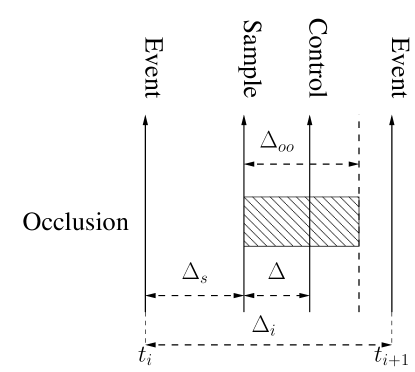
Figure 3: Self-occlusion. Following an event, the observer is sampled at a time $\Delta_{s}$ and a new control trajectory is generated. The observer is then occluded for a further time $\Delta_{oo}=\Delta_{o}$ where $\Delta_{o}$ is the internal occlusion interval. Following that time, the observer is operational and an event can be detected (3.20). The actual time between events $\Delta_{i}>\Delta_{s}+\Delta_{oo}$

The intermittent controller of Gawthrop et al. (2011) uses continuous observation however, motivated by the occlusion experiments of Osborne (2013), this chapter looks a intermittent observation.

As discussed in Section 3.2, the predictor state ${\mathbf{x}_{p}}$ is only sampled at discrete-times $t_{i}$. Further, from Equation (2.5), ${\mathbf{x}_{p}}$ is a function of ${\mathbf{x}_{o}}$ at these times. Thus the only the observer performance at the discrete-times $t_{i}$ is important. With this in mind, this Chapter proposes, in the context of intermittent control, that the continuous observer is replaced by an intermittent observer where periods of monitoring the system measurements are interleaved with periods where the measurement is occluded. In particular, and with reference to Figure 3, this Chapter examines the situation where observation is occluded for a time $\Delta_{oo}$ following sampling. Such occlusion is equivalent to setting the observer gain $L=0$ in Equation (2.2). Setting $L=0$ has two consequences: the measured signal $y$ is ignored and the observer state evolves as the disturbance-free system.

With reference to Equation (3.8); the intermittent controller only makes use of the state estimate at the discrete time points at $t=t^{s}_{i}$ (3.2); moreover, in the event-driven case, the observer state estimate is used in Equation (3.20) to determine the event times $t_{i}$ and thus $t^{s}_{i}$. Hence, a good state estimate immediately after an sample at time $t^{s}_{i}$ is not required and so one would expect that occlusion ($L=0$) would have little effect immediately after $t=t^{s}_{i}$. For this reason, define the occlusion time. $\Delta_{oo}$ as the time after $t=t^{s}_{i}$ for which the observer is open-loop $L=0$. That is, the constant observer gain is replaced by the time varying observer gain:

$$L(t)=\begin{cases}0&\tau^{s}<\Delta_{oo}\\ L_{o}&\tau^{s}\geq\Delta_{oo}\end{cases}$$ (3.9)

where $L_{o}$ is the observer gain designed using standard techniques (Kwakernaak and Sivan, 1972; Goodwin et al., 2001) and the intermittent time $\tau^{s}$ is given by (3.4).

3.4 Intermittent predictor

The continuous-time predictor of equation (2.5) contains a convolution integral which, in general, must be approximated for real-time purposes and therefore has a speed-accuracy trade-off. This section shows that the use of intermittent control, together with the hold of Section 3.2, means that equation (2.5) can be replaced by a simple exact formula.

Equation (2.5) is the solution of the differential equation (in the intermittent time $\tau$ (3.3) time frame)

$$\begin{cases}\frac{d}{d\tau}{{{\mathbf{x}_{p}}}}(\tau)&=\mathbf{A}{\mathbf{x}_{p}}(\tau)+\mathbf{B}u(\tau)\\ {\mathbf{x}_{p}}(0)&={\mathbf{x}_{w}}(t^{s}_{i})\end{cases}$$ (3.10)

evaluated at time $\tau^{s}=\Delta$ where $\tau^{s}_{i}$ is given by Equation (3.2). However, the control signal $\mathbf{u}$ is not arbitrary but rather given by the hold equation (3.6). Combining equations (3.6) and (3.10) gives

$$\begin{cases}\frac{d}{d\tau}{\mathbf{X}}(\tau)&=\mathbf{A}_{ph}\mathbf{X}(\tau)\\ \mathbf{X}(0)&=\mathbf{X}_{i}\end{cases}$$ (3.11)

where

$$\mathbf{X}(\tau) =\begin{pmatrix}{\mathbf{x}_{p}}(\tau)\\ {\mathbf{x}_{h}}(\tau)\end{pmatrix}$$ (3.12)

$$\mathbf{X}_{i} =\begin{pmatrix}{\mathbf{x}_{w}}(t_{i})\\ {\mathbf{x}_{p}}(t_{i}-\Delta)\end{pmatrix}$$ (3.13)

$$\text{and }\mathbf{A}_{ph} =\begin{pmatrix}\mathbf{A}&-\mathbf{B}\mathbf{k}\\ {{\mathbf{0}}}_{n\times n}&\mathbf{A}_{h}\end{pmatrix}$$ (3.14)

where ${{\mathbf{0}}}$ is a zero matrix of the indicated dimensions and the hold matrix $\mathbf{A}_{h}$ can be $\mathbf{A}_{c}$ (SMH) or ${{\mathbf{0}}}$ (ZOH).

The equation (3.11) has an explicit solution at time $\tau=\Delta$ given by:

$$\mathbf{X}(\Delta)=e^{\mathbf{A}_{ph}\Delta}\mathbf{X}_{i}$$ (3.15)

The prediction ${\mathbf{x}_{p}}$ can be extracted from (3.15) to give:

$${\mathbf{x}_{p}}(t_{i})=\mathbf{E}_{pp}{\mathbf{x}_{w}}(t_{i})+\mathbf{E}_{ph}{\mathbf{x}_{h}}(t_{i})$$ (3.16)

where the $n\times n$ matrices $\mathbf{E}_{pp}$ and $\mathbf{E}_{ph}$ are partitions of the $2n\times 2n$ matrix $\mathbf{E}$:

$$\mathbf{E} =\begin{pmatrix}\mathbf{E}_{pp}&\mathbf{E}_{ph}\\ \mathbf{E}_{hp}&\mathbf{E}_{hh}\end{pmatrix}$$ (3.17)

$$\text{where }\mathbf{E} =e^{\mathbf{A}_{ph}\Delta}$$ (3.18)

The intermittent predictor (3.16) replaces the continuous-time predictor (2.5); there is no convolution involved and the matrices $\mathbf{E}_{pp}$ and $\mathbf{E}_{ph}$ can be computed off-line and so do not impose a computational burden in real-time.

3.5 State feedback

The “state-feedback” block of Figure 2 is implemented as:

$$\mathbf{u}(t)=-\mathbf{k}\mathbf{x}_{h}(t)$$ (3.19)

This is similar to the conventional state feedback of Figure 1 given by Equation (2.7) but the continuous predicted state ${\mathbf{x}_{w}}(t)$ is repaces by the hold state $\mathbf{x}_{h}(t)$ generated by Equation (3.6).

3.6 Event detector

The purpose of the event detector is to generate the intermittent sample times $t_{i}$ and thus trigger feedback. Such feedback is required when the open-loop hold state ${\mathbf{x}_{h}}$ (3.6) differs significantly from the closed-loop observer state ${{\mathbf{x}}_{w}}$ (2.15) indicating the presence of disturbances. There are many ways to measure such a discrepancy; following Gawthrop et al. (2011), the one chosen here is to look for a quadratic function of the error $\mathbf{e}_{hp}$ exceeding a threshold $q_{t}^{2}$:

$$E =\mathbf{e}_{hp}^{T}(t)\mathbf{Q}_{t}\mathbf{e}_{hp}(t)-q_{t}^{2}\geq 0$$ (3.20)

$$\text{where }\mathbf{e}_{hp}(t) ={\mathbf{x}_{h}}(t)-{{\mathbf{x}}_{w}}(t)$$ (3.21)

where $\mathbf{Q}_{t}$ is a positive semi-definite matrix.

3.7 The intermittent-equivalent setpoint

Loram et al. (2012) introduce the concept of the equivalent setpoint for intermittent control. This section extends the concept and there are two differences:

1. the setpoint sampling occurs at $t_{i}+\Delta_{s}$ rather than at $t_{i}$ and

2. the filtered setpoint $\mathbf{w}_{f}$ (rather than $\mathbf{w}$) is sampled.

Define the sample time $t^{s}_{i}$ (as opposed to the event time $t_{i}$ and the corresponding intermittent time $\tau^{s}$ by

$$t^{s}_{i} =t_{i}+\Delta_{s}$$ (3.22)

$$\tau^{s} =\tau-\Delta_{s}=t-t_{i}-\Delta_{s}=t-t^{s}_{i}$$ (3.23)

In particular, the sampled setpoint $\mathbf{w}_{s}$ becomes:

$$\mathbf{w}_{s}(t)=\mathbf{w}_{f}(t^{s}_{i})\text{ for $t^{s}_{i}\leq t<t^{s}_{i+1}$}$$ (3.24)

where $\mathbf{w}_{f}$ is the filtered setpoint $\mathbf{w}$. That is the sampled setpoint $\mathbf{w}_{s}$ is the filtered setpoint at time $t^{s}_{i}=t_{i}+\Delta_{s}$.

The equivalent setpoint $\mathbf{w}_{ic}$ is then given by:

$$\mathbf{w}_{ic}(t) =\mathbf{w}_{s}(t-t_{d})$$ (3.25)

$$=\mathbf{w}_{f}(t^{s}_{i}-t_{d})$$ (3.26)

$$=\mathbf{w}_{f}(t-\tau^{s}-t_{d})\text{ for $t^{s}_{i}\leq t<t^{s}_{i+1}$}$$ (3.27)

This corresponds to the previous result (Loram et al., 2012) when $\Delta_{s}=0$ and $\mathbf{w}_{f}(t)=\mathbf{w}(t)$.

If, however, the setpoint $\mathbf{w}(t)$ is such that $\mathbf{w}_{f}(t^{s}_{i})\approx\mathbf{w}(t_{s})$ (ie no second stimulus within the filter settling time and $\Delta_{s}$ is greater than the filter settling time) then Equation (3.25) may be approximated by:

$$\mathbf{w}_{ic}(t) \approx\mathbf{w}(t^{s}_{i}-t_{d})\text{ for $t^{s}_{i}\leq t<t^{s}_{i+1}$}$$ (3.28)

$$=\mathbf{w}(t-\tau^{s}-t_{d})\text{ for $t^{s}_{i}\leq t<t^{s}_{i+1}$}$$ (3.29)

As discussed in Section 10, the intermittent-equivalent setpoint is the basis for identification of intermittent control.

3.8 The intermittent separation principle.

As discussed in Section 3.2, the Intermittent Controller contains a System-Matched Hold which can be views as a particular form of generalised hold (Gawthrop and Wang, 2007). Insofar as this special case of intermittent control uses a dynamical model of the controlled system to generate the (open-loop) control between sample intervals, it is related to the strategies of both Zhivoglyadov and Middleton (2003) and Astrom (2008). However, as shown in this chapter, intermittent control provides a framework within which to analyse and design a range of control systems with unpredictable non-uniform sampling possibly arising from an event-driven design.

In particular, it is shown by Gawthrop and Wang (2011), that the SMH-based intermittent controller is associated with a separation principle similar to that of the underlying continuous-time controller, which states that the closed-loop poles of the intermittent control system consist of the control system poles and the observer system poles, and the interpolation using the system matched hold does not lead to the changes of closed-loop poles. As discussed by Gawthrop and Wang (2011), this separation principle is only valid when using the SMH. For example, intermittent control based on the standard zero-order hold (ZOH) does not lead to such a separation principle and therefore closed-loop stability is compromised when the sample interval is not fixed.

As discussed by Gawthrop and Wang (2011), an important consequence of this separation principle is that the neither the design of the SMH, nor the stability of the closed-loop system in the fixed sampling case, is dependent on sample interval. It is therefore conjectured that the SMH is particularly appropriate when sample times are unpredictable or non-uniform, possibly arising from an event-driven design.

4 Examples: basic properties of intermittent control

This section uses simulation to illustrate key properties of intermittent control. Section 4.1 illustrates

• timed & event-driven control (Section 3.6),

• the roles of the disturbance observer and series integrator (Section 2.1),

• the choice of event threshold (Section 3.6),

• the difference between control-delay & sampling delay (Section 3.1),

• the effect of low & high observer gain (Section 2.1) and

• the effect of occlusion (Section 3.4).

Sections 4.2 and 4.3 illustrates how the intermittent controller models two basic psychological phenomenon: the Psychological Refractory Period and the Amplitude Transition Function.

4.1 Elementary examples

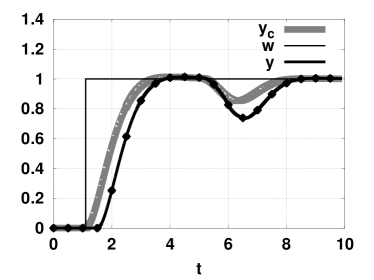
(a) Timed: $y$

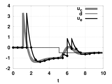
(b) Timed: $u$

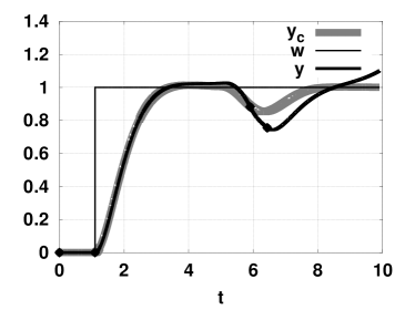
(c) Event-driven: $y$

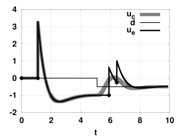
(d) Event-driven: $u$

Figure 4: Elementary example: timed & event-driven

This section illustrates the basic properties of intermittent control using simple examples. In all cases, the system is given by:

$$G_{0}(s) =\frac{1}{s^{2}-1}=\frac{1}{(s-1)(s+1)}$$ Second-order unstable system (4.1)

$$G_{v}(s) =\frac{1}{s}$$ Simple integrator for disturbance observer (4.2)

The corresponding state-space system (2.1) is:

$$\mathbf{A} =\begin{pmatrix}0&0&1\\ 1&0&0\\ 0&0&0\end{pmatrix}$$ (4.3)

$$\mathbf{B} =\mathbf{B}_{d}=\begin{pmatrix}1\\ 0\\ 0\end{pmatrix}$$ (4.4)

$$\mathbf{B}_{v} =\begin{pmatrix}0\\ 0\\ 1\end{pmatrix}$$ (4.5)

$$\mathbf{C} =\begin{pmatrix}0&1&0\end{pmatrix}$$ (4.6)

All signals are zero except:

$$w(t) =1 t\geq 1.1$$ (4.7)

$$d(t) =0.5 t\geq 5.1$$ (4.8)

Except where stated, the intermittent control parameters are:

$$\Delta_{min} =0.5 \text{Min. intermittent interval}~{}(\ref{eq:PRP})$$

$$q_{t} =0.1 \text{Threshold}(\ref{eq:ED_e})~{}$$

$$\Delta =0 \text{Control delay}(\ref{eq:pred})~{}$$

$$\Delta_{s} =0 \text{Sampling delay}(\ref{eq:t_s_i})~{}$$

Figures 4– 9 are all of the same format. The left column of figures shows the system output $y$ together with the setpoint $w$ and the output $y_{c}$ corresponding to the underlying continuous-time design; the right column shows the corresponding control signal $u_{e}$ together with the negative disturbance $-d$ and the control $u_{c}$. In each case the $\bullet$ symbol corresponds to an event.

Figure 4 contrasts timed and event driven control. In particular, Figures 4(a) and 4(b) correspond to zero threshold ($q_{t}=0$) and thus timed intermittent control with fixed interval $\Delta_{min}=0.5$ and Figures 4(c) and 4(d) correspond to event-driven control. The event driven case has two advantages: the controller responds immediately to the setpoint change at time $t=1.1$ whereas the timed case has to wait until the next sample at $t=1.5$ and the control is only computed when required. In particular, the initial setpoint response does not need to be corrected, but the unknown disturbance means that the observer state is different from the system state for a while and so corrections need to be made until the disturbance is correctly deduced by the observer.

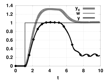
(a) No integrator: $y$

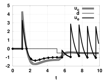
(b) No integrator: $u$

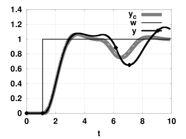
(c) Integrator: $y$

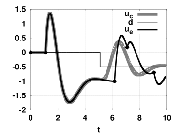
(d) Integrator: $u$

Figure 5: Elementary example: no disturbance observer, with and without integrator

The simulation of Figure 4 includes the disturbance observer implied by the integrator of Equation 4.2; this means that the controllers are able to asymptotically eliminate the constant disturbance $d$. Figures 5(a) and 5(b) show the effect of not using the disturbance observer. The constant disturbance $d$ is not eliminated and the intermittent controller exhibits limit cycling behaviour (analysed further by Gawthrop (2009)). As an alternative to the disturbance observer used in the simulation of Figure 4, a series integrator can be used by setting:

$$G_{s}(s) =\frac{1}{s}$$ Series integrator for disturbance rejection (4.9)

The corresponding simulation is shown in Figures 5(c) and 5(d). Although the constant disturbance $d$ is now asymptotically eliminated, the additional integrator increases both the system order and the system relative degree by one giving a more difficult system to control.

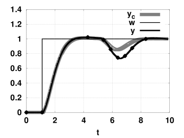
(a) Low threshold: $y$

(b) Low threshold: $u$

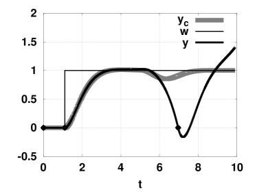
(c) High threshold: $y$

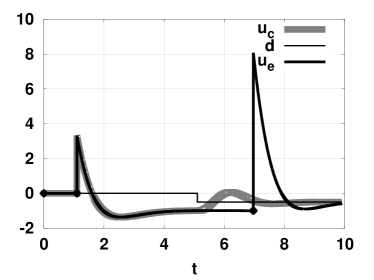
(d) High threshold: $u$

Figure 6: Elementary example: low & high threshold

The event detector behaviour depends on the threshold $q_{t}$ (3.20); this has already been examined in the simulations of Figure 4. Figure 6 shows the effect of a low ($q_{t}=0.01$) and high ($q_{t}=1$) threshold. As discussed in the context of Figure 4, the initial setpoint response does not need to be corrected, but the unknown disturbance generates events. The simulations of Figure 6 indicate the trade-off between performance and event rate determined by the choice of the threshold $q_{t}$.

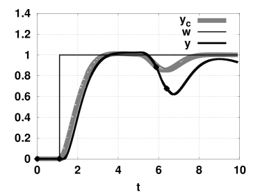
(a) Control delay: $y$

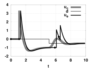
(b) Control delay: $u$

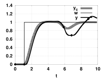
(c) Sample delay: $y$

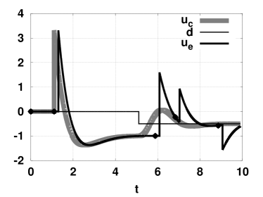
(d) Sample delay: $u$

Figure 7: Elementary example: control-delay & sampling delay

The simulations of Figure 7 compare and contrast the two delays: control delay $\Delta$ and sample delay $\Delta_{s}$. In particular, Figures 7(a) and 7(b) correspond to $\Delta=0.4$ and $\Delta_{s}=0$ but Figures 7(c) and 7(d) correspond to $\Delta=0$ and $\Delta_{s}=0.4$. The response to the setpoint is identical as the prediction error is zero in this case; the response to the disturbance change is similar, but not identical as the prediction error is not zero in this case.

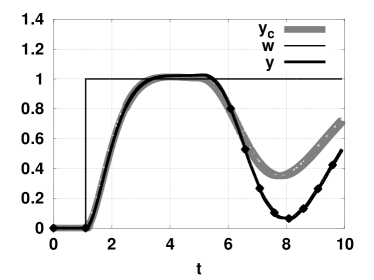
(a) Low observer gain: $y$

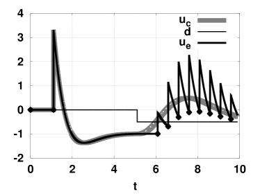
(b) Low observer gain: $u$

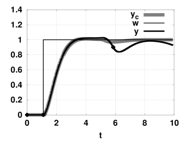
(c) High observer gain: $y$

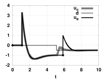
(d) High observer gain: $u$

Figure 8: Elementary example: low & high observer gain

The state observer of Equation (2.2) is needed to deduce unknown states in general and the state corresponding to the unknown disturbance in particular. As discussed in the textbooks (Kwakernaak and Sivan, 1972; Goodwin et al., 2001), the choice of observer gain gives a trade-off between measurement noise and disturbance responses. The gain used in the simulations of Figure 4 can be regarded as medium; Figure 8 looks at low and high gains. As there is no measurement noise in this case, the low gain observer gives a poor disturbance response whilst the high gain gives an improved disturbance response.

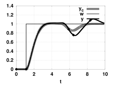
(a) Low occlusion time: $y$

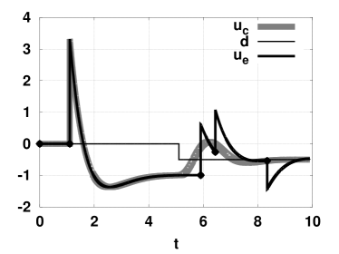
(b) Low occlusion time: $u$

(c) High occlusion time: $y$

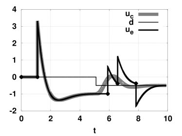
(d) High occlusion time: $u$

Figure 9: Elementary example: low & high occlusion time

The simulations presented in Figure 9 investigate the intermittent observer of Section 3.3. In particular, the measurement of the system output $y$ is assumed to be occluded for a period $\Delta_{oo}$ following a sample. Figures Figures 9(a) and 9(b) show simulation with $\Delta_{oo}=0.1$ and Figures Figures 9(c) and 9(d) show simulation with $\Delta_{oo}=0.5$. It can be seen that occlusion has little effect on performance for the lower value, but performance is poor for the larger value.

4.2 The Psychological Refractory Period and Intermittent-equivalent setpoint

As noted in Section 3.7, the intermittent sampling of the setpoint $w$ leads to the concept of the intermittent-equivalent setpoint: the setpoint that is actually used within the intermittent controller. Moreover, as noted in Section 3.1, there is a minimum intermittent interval $\Delta_{min}$. As discussed by Gawthrop et al. (2011), $\Delta_{min}$ is related to the psychological refractory period (PRP) (Telford, 1931) which explains the experimental results of Vince (1948) where a second reaction time may be longer that the first. These ideas are explored by simulation in Figures 10– 12. In all cases, the system is given by:

$$G_{0}(s) =\frac{1}{s}$$ Simple integrator (4.10)

The corresponding state-space system (2.1) is:

$$\mathbf{A} =0,\;\mathbf{B}=\mathbf{C}=1$$ (4.12)

All signals are zero except the signal $w_{0}$ is defined as:

$$w_{0}(t) =1 0.5\leq t\leq 1.5,\;2.0\leq t\leq 2.5,\;3.0\leq t\leq 3.2,\;4.0\leq t\leq 4.1$$ (4.13)

and the filtered setpoint $w$ is obtained by passing $w$ through the low-pass filter $G_{w}(s)$ where:

$$G_{w}(s)=\frac{1}{1+sT_{f}}$$ (4.14)

Except where stated, the intermittent control parameters are:

$$\Delta_{min} =0.5 \text{Min. intermittent interval}~{}(\ref{eq:PRP})$$

$$q_{t} =0.1 \text{Threshold}(\ref{eq:ED_e})~{}$$

$$\Delta =0 \text{Control delay}(\ref{eq:pred})~{}$$

$$\Delta_{s} =0 \text{Sampling delay}(\ref{eq:t_s_i})~{}$$

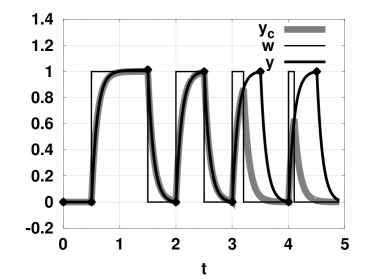
(a) Intermittent control

(b) Intermittent-equivalent setpoint

Figure 10: Psychological Refractory Period: square setpoint

Figure 10(a) corresponds to the unfiltered setpoint with $T_{f}=0$ and $w=w_{0}$ where $w_{0}$ is given by (4.13). For the first two (wider) pulses, events ($\bullet$) occur at each setpoint change; but the second two (narrower) pulses, the trailing edges occur at a time less that $\Delta_{min}=0.5$ from the leading edges and thus the events corresponding to the trailing edges are delayed until $\Delta_{min}$ has elapsed. Thus the the second two (narrower) pulse lead to outputs as if the pulses were $\Delta_{min}$ wide. Figure 10(b) shows the intermittent-equivalent setpoint $w_{ic}$ superimposed on the actual setpoint $w$.

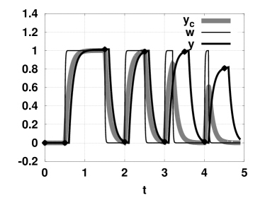
(a) Intermittent control

(b) Intermittent-equivalent setpoint

Figure 11: Psychological Refractory Period: filtered setpoint

Figure 11(a) corresponds to the filtered setpoint with $T_{f}=0.01$ and $w=w_{0}$ where $w_{0}$ is given by (4.13). At the event times, the setpoint has not yet reached its final value and thus the initial response is too small which is then corrected; Figure 11(b) shows the intermittent-equivalent setpoint $w_{ic}$ superimposed on the actual setpoint $w$.

(a) Intermittent control

(b) Intermittent-equivalent setpoint

Figure 12: Psychological Refractory Period: sampling delay

The unsatisfactory behaviour can be improved by delaying the sample time by $\Delta_{s}$ as discussed in Section 3.1. Figure 12(a) corresponds to Figure 11(a) exept that $\Delta_{s}=0.1$. Except for the short delay of $\Delta_{s}=0.1$, the behavior of the first three pulses is now similar to that of Figure 10(a). The fourth (shortest) pulse gives, however, a reduced amplitude output; this is because the sample occurs on the trailing edge of the pulse. This behavior has been observed by Vince (1948) as is related to the Amplitude Transition Function of Barrett and Glencross (1988). Figure 12(b) shows the intermittent-equivalent setpoint $w_{ic}$ superimposed on the actual setpoint $w$. This phenomena is further investigated in Section 4.3.

4.3 The Amplitude Transition Function

(a) $y\&w$: Pulse width $200$ms

(b) $y\&w$: Pulse width $100$ms

Figure 13: Amplitude Transition Function.

This section exands on the observation in Section 4.2, Figure 12, that the combination of sampling delay and a bandwifth limited setpoint can lead to narrow pulses being “missed”. It turns out that the physiological equivalent of this behaviour is the so called Amplitude Transition Function (ATF) described by Barrett and Glencross (1988). Instead of the symmetric pulse discussed in the PRP context in Section 4.2, the ATF concept is based on asymmetric pulses where the step down is less than the step up leading to a non-zero final value. An example of an asymetric pulse appears in Figure 13 The simulations in this section use the same system as in Section 4.2 Equations (4.10) and (4.12), but the setpoint $w_{0}$ of Equation (4.13) is replaced by:

$$w_{0}(t)=\begin{cases}0&t<1\\ 1&1\leq t\leq 1+\Delta_{p}\\ 0.5&t>1+\Delta_{p}\end{cases}$$ (4.15)

where $\Delta_{p}$ is the pulse-width.

The system was simulated for two pulse widths: $\Delta_{p}=200$ms (Figure 13(a)) and $\Delta_{p}=100$ms (Figure 13(b)). In each case, following Equation (4.15), the pulse was asymmetric going from 0 to 1 and back to 0.5.

At each pulse width, the system was simulated with event delay $\Delta_{s}=90,100,\dots,150$ms and the control delay was set to $100$ms. Figure 13(a) shows the “usual” behaviour, the 200ms pulse is expanded to $\Delta_{ol}=500$ms and delayed by $\Delta+\Delta_{s}$. In contrast, Figure 13(a) shows the “Amplitude Transition Function” behaviour: because the sampling is occurring on the downwards side of the pulse, the amplitude is reduced with increasing $\Delta_{s}$. Figure 13(a) is closely related to Figure 2 of Barrett and Glencross (1988).

5 Constrained design

The design approach outlined in Sections 2 and 3 assumes that system inputs and outputs can take any value. In practice, this is not always the case and so constraints on both system inputs and outputs must be taken into account. There are at least three classes of contraints of interest in the context of intermittent control:

1. Constraints on the steady-state behaviour of a system. These are particularly relevant in the context of multi-input ($n_{u}>1$) and multi-output ($n_{y}>1$) systems. This issue is discussed in Section 5.1 and illustrated by example in Section 7.

2. Amplitude constraints on the dynamical behaviour of a system. This is a topic that is much dicussed in the Model Predictive Control literature – for example (Rawlings, 2000; Maciejowski, 2002; Wang, 2009). In the context of intermittent control, constraints have been considered in the single-input single-output context by Gawthrop and Wang (2009a); the corresponding multivariable case is considered in Section 5.2 and illustrated in Section 6.

3. Power constraints on the dynamical behaviour of a system. This topic has been discussed by Gawthrop et al. (2013c).

5.1 Constrained Steady-State Design

Section 2.4 considers the steady state design of the continuous controller underlying intermittent control. In particular, Equation (2.13) gives a linear algebraic equation giving the steady-state system state ${\mathbf{x}}_{ss}$ and corresponding control signal ${\mathbf{u}}_{ss}$ yeilding a particular steady-state output ${\mathbf{y}}_{ss}$. Although in the single-input single-output case considered by Gawthrop et al. (2011, Equation 13) the solution is unique, as discussed in Section 2.4 the multi-input, multi-output case gives rise to more possibilities. In particular, it is not possible to exactly solve Equation (2.13) in the over-determined case where $n_{ss}>n_{u}$, but a least-squares solution exists. In the constrained case, this solution must satisfy two sets of constraints: an equality constraint ensuring that the equilibrium condition (2.10) holds and inequality constraints to reject physically impossible solutions.

In this context, the $n_{ss}\times n_{ss}$ weighting matrix $\mathbf{Q}_{ss}$ can be used to vary the relative importance each element of ${\mathbf{y}}_{ss}$. In particular, define:

$$\mathbf{S}_{\mathbf{Q}} =\begin{bmatrix}\mathbf{A}&\mathbf{B}\\ \mathbf{Q}_{ss}\mathbf{C}_{ss}&{{\mathbf{0}}}_{n_{ss}\times n_{u}}\end{bmatrix}$$ (5.1)

$${\mathbf{X}}_{ss} =\begin{bmatrix}{\mathbf{x}}_{ss}\\ {\mathbf{u}}_{ss}\end{bmatrix}$$ (5.2)

$${\mathbf{y}}_{ss} =\begin{bmatrix}-\mathbf{B}_{d}{\mathbf{d}}_{ss}\\ \mathbf{Q}_{ss}{\mathbf{y}}_{ss}\end{bmatrix}$$ (5.3)

$$\text{and }\hat{\mathbf{Y}}_{ss} =\begin{bmatrix}-\mathbf{B}_{d}{\mathbf{d}}_{ss}\\ \mathbf{Q}_{ss}\hat{\mathbf{y}}_{ss}\end{bmatrix}=\mathbf{S}_{\mathbf{Q}}\hat{\mathbf{X}}_{ss}$$ (5.4)

This gives rise to the least-squares cost function:

$$J_{ss} =\left({\mathbf{y}}_{ss}-\hat{\mathbf{Y}}_{ss}\right)^{T}\left({\mathbf{y}}_{ss}-\hat{\mathbf{Y}}_{ss}\right)$$

$$=\left({\mathbf{y}}_{ss}-\mathbf{S}_{\mathbf{Q}}\hat{\mathbf{X}}_{ss}\right)^{T}\left({\mathbf{y}}_{ss}-\mathbf{S}_{\mathbf{Q}}\hat{\mathbf{X}}_{ss}\right)$$ (5.5)

Differentiating with respect to $\hat{\mathbf{X}}_{ss}$ gives the weighted least-squares solution of (2.13):

$$\mathbf{S}_{\mathbf{Q}}^{T}\left({\mathbf{y}}_{ss}-\mathbf{S}_{\mathbf{Q}}\hat{\mathbf{X}}_{ss}\right) =0$$ (5.6)

$$\text{or }\hat{\mathbf{X}}_{ss} =\left(\mathbf{S}_{\mathbf{Q}}^{T}\mathbf{S}_{\mathbf{Q}}\right)^{-1}\mathbf{S}_{\mathbf{Q}}^{T}{\mathbf{y}}_{ss}$$ (5.7)

As ${\mathbf{x}}_{ss}$ corresponds to a steady state solution corresponding to Equation (2.10), the solution of the least-squares problem is subject to the equality constraint:

$$\begin{bmatrix}\mathbf{A}&\mathbf{B}\end{bmatrix}\hat{\mathbf{X}}_{ss}=\mathbf{A}{\mathbf{x}}_{ss}+\mathbf{B}{\mathbf{u}}_{ss}=-\mathbf{B}_{d}{\mathbf{d}}_{ss}$$ (5.8)

Furthermore, suppose that the solution must be such that the components of $\mathbf{Y}$ corresponding to ${\mathbf{y}}_{ss}$ are bounded above and below:

$$\hat{\mathbf{y}}_{min}\leq\hat{\mathbf{y}}=\mathbf{C}_{ss}\hat{\mathbf{X}}\leq\hat{\mathbf{y}}_{max}$$ (5.9)

Inequality (5.9) can be rewritten as:

$$\begin{bmatrix}-\mathbf{C}_{ss}\\ \mathbf{C}_{ss}\end{bmatrix}\hat{\mathbf{X}}\leq\begin{bmatrix}-\hat{\mathbf{y}}_{min}\\ \hat{\mathbf{y}}_{max}\end{bmatrix}$$ (5.10)

The quadratic cost function (5.5) together with the linear equality constraint (5.8) and the linear inequality constraint (5.10) forms a quadratic program (QP) which has well-established numerical algorithms available for its solution (Fletcher, 1987).

An example of constrained steady-state optimisation is given in Section 7.5.

5.2 Constrained Dynamical Design

Model-based predictive control (MPC) (Rawlings, 2000; Maciejowski, 2002; Wang, 2009) combines a quadratic cost function with linear constraints to provide optimal control subject to (hard) constraints on both state and control signal; this combination of quadratic cost and linear constraints can be solved using quadratic programming (QP) (Fletcher, 1987; Boyd and Vandenberghe, 2004). Almost all MPC algorithms have a discrete-time framework. As a move towards a continuous-time formulation of intermittent control, the intermittent approach to MPC was introduced (Ronco et al., 1999) to reduce on-line computational demand whilst retaining continuous-time like behaviour (Gawthrop and Wang, 2007, 2009a; Gawthrop et al., 2011). This section introduces and illustrates this material.

Using the feedback control comprising the system matched hold (3.6), its initialisation (3.8), and feedback (3.19) may cause state or input constraints to be violated over the intermittent interval. The key idea introduced by Chen and Gawthrop (2006) and exploited by Gawthrop and Wang (2009a) is to replace the SMH initialisation (at time $t=t_{i}$ (3.1)) of Equation (3.8) by:

$${\mathbf{x}_{h}}(0) =\begin{cases}{{\mathbf{x}}_{p}}(t_{i}-\Delta)-{\mathbf{x}}_{ss}w(t_{i})&\text{when constraints not violated}\\ \mathbf{U}_{i}&\text{otherwise}\end{cases}$$ (5.11)

where $\mathbf{U}_{i}$ is the result of the on-line optimisation to be discussed in Section 5.2.2.

The first step is to construct a set of equations describing the evolution of the system state $\mathbf{x}$ and the generalised hold state $\mathbf{x}_{h}$ as a function of the initial states and assuming that disturbances are zero.

The differential equation (3.11) has the explicit solution

$$\mathbf{X}(\tau) =\mathbf{E}(\tau)\mathbf{X}_{i}$$ (5.12)

$$\text{where }\mathbf{E}(\tau) =e^{\mathbf{A}_{xu}\tau}$$ (5.13)

where $\tau$ is the intermittent continuous-time variable based on $t_{i}$.

5.2.1 Constraints

The vector $\mathbf{X}$ (3.11) contains the system state and the state of the generalised hold; equation (5.12) explicitly give $\mathbf{X}$ in terms of the system state $\mathbf{x}_{i}(t_{i})$ and the hold state ${\mathbf{x}_{h}}(t_{i})=\mathbf{U}_{i}$ at time $t_{i}$. Therefore any constraint expressed at a future time $\tau$ as a linear combination of $\mathbf{X}$ can be re-expressed in terms of ${\mathbf{x}_{h}}$ and $\mathbf{U}_{i}$. In particular if the constraint at time $\tau$ is expressed as:

$$\Gamma_{\tau}\mathbf{X}(\tau)\leq\gamma_{\tau}$$ (5.14)

where $\Gamma_{\tau}$ is a $2n$-dimensional row vector and $\gamma_{\tau}$ a scalar then the constraint can be re expressed using (5.12) in terms of the intermittent control vector $\mathbf{U}_{i}$ as:

$$\Gamma_{\tau}E_{u}(\tau)\mathbf{U}_{i}\leq\gamma_{\tau}-\Gamma_{\tau}E_{x}(\tau)\mathbf{x}_{i}$$ (5.15)

where $E$ has been partitioned into the two $2n\times n$ sub-matrices $E_{x}$ and $E_{u}$ as:

$$E(\tau)=\begin{pmatrix}E_{x}(\tau)&E_{u}(\tau)\end{pmatrix}$$ (5.16)

If there are $n_{c}$ such constraints, they can be combined as:

$$\Gamma\mathbf{U}_{i}\leq\gamma-\Gamma_{x}\mathbf{x}_{i}$$ (5.17)

where each row of $\Gamma$ is $\Gamma_{\tau}E_{u}(\tau)$, each row of $\Gamma_{x}$ is $\Gamma_{\tau}E_{x}(\tau)$ and each (scalar) row of $\gamma$ is $\gamma_{\tau}$.

Following standard MPC practice, constraints beyond the intermittent interval can be included by assuming that the the control strategy will be open-loop in the future.

5.2.2 Optimisation

Following, for example, Chen and Gawthrop (2006), a modified version of the infinite-horizon LQR cost (2.6) is used:

$$J_{ic}=\int_{0}^{\tau_{1}}\mathbf{x}(\tau)^{T}\mathbf{Q}\mathbf{x}(\tau)+u(\tau)\mathbf{R}u(\tau)\,d\tau+\mathbf{x}(\tau_{1})^{T}{\mathbf{P}}\mathbf{x}(\tau_{1})$$ (5.18)

where the weighting matrices $\mathbf{Q}$ and $\mathbf{R}$ are as used in (2.6) and ${\mathbf{P}}$ is the positive-definite solution of the algebraic Riccati equation (ARE):

$$\mathbf{A}^{T}{\mathbf{P}}+{\mathbf{P}}\mathbf{A}-{\mathbf{P}}\mathbf{B}\mathbf{R}^{-1}\mathbf{B}^{T}{\mathbf{P}}+\mathbf{Q}=0$$ (5.19)

There are an number of differences between our approach to minimising $J_{ic}$ (5.18) and the LQR approach to minimising $J_{LQR}$ (2.6).

1. Following the standard MPC approach (Maciejowski, 2002), this is a receding-horizon optimisation in the time frame of $\tau$ not $t$.

2. The integral is over a finite time $\tau_{1}$.

3. A terminal cost is added based on the steady-state ARE (5.19). In the discrete-time context, this idea is due to Rawlings and Muske (1993).

4. The minimisation is with respect to the intermittent control vector $\mathbf{U}_{i}$ generating the the control signal $u$ (2.7) through the generalised hold (3.6).

Using $\mathbf{X}$ from (5.12), (5.18) can be rewritten as

$$J_{ic} =\int_{0}^{\tau_{1}}\mathbf{X}(\tau)^{T}\mathbf{Q}_{xu}\mathbf{X}(\tau)\,d\tau+\mathbf{X}(\tau_{1})^{T}{\mathbf{P}}_{xu}\mathbf{X}(\tau_{1})$$ (5.20)

$$\text{where }\mathbf{Q}_{xu} =\begin{pmatrix}\mathbf{Q}&0_{n\times n}\\ 0_{n\times n}&\mathbf{x}_{uo}\mathbf{R}\mathbf{x}_{uo}^{T}\end{pmatrix}$$ (5.21)

$$\text{and }{\mathbf{P}}_{xu} =\begin{pmatrix}{\mathbf{P}}&0_{n\times n}\\ 0_{n\times n}&0_{n\times n}\end{pmatrix}$$ (5.22)

Using (5.12), equation (5.20) can be rewritten as:

$$J_{ic} =\mathbf{X}_{i}^{T}J_{XX}\mathbf{X}_{i}$$ (5.23)

$$\text{where }J_{XX} =J_{1}+e^{\mathbf{A}_{xu}^{T}\tau_{1}}{\mathbf{P}}_{xu}e^{\mathbf{A}_{xu}\tau_{1}}$$ (5.24)

$$\text{and }J_{1} =\int_{0}^{\tau_{1}}e^{\mathbf{A}_{xu}^{T}\tau}\mathbf{Q}_{xu}e^{\mathbf{A}_{xu}\tau}\,d\tau$$ (5.25)

The $2n\times 2n$ matrix $J_{XX}$ can be partitioned into four $n\times n$ matrices as:

$$J_{XX}=\begin{pmatrix}J_{xx}&J_{xU}\\ J_{Ux}&J_{UU}\end{pmatrix}$$ (5.26)

Lemma 1 (Constrained optimisation)

The minimisation of the cost function $J_{ic}$ of Equation 5.18 subject to the constraints (5.17) is equivalent to the solution of the quadratic programme for the optimum value of $\mathbf{U}_{i}$:

$$\min_{U_{i}}\left\{\mathbf{U}_{i}^{T}J_{UU}\mathbf{U}_{i}+\mathbf{x}_{i}^{T}J_{Ux}\mathbf{U}_{i}\right\}$$ (5.27)

$\text{ subject to }\Gamma\mathbf{U}_{i}\leq\gamma-\Gamma_{x}\mathbf{x}_{i}$ where $J_{UU}$ and $J_{Ux}$ are given by (5.26) and $\Gamma$, $\Gamma_{x}$ and $\gamma$ as described in Section 5.2.1.

Proof 1

See (Chen and Gawthrop, 2006).

Remarks.

1. This optimisation is dependant on the system state $\mathbf{x}$ and therefore must be accomplished at every intermittent interval $\Delta_{i}$.

2. The computation time is reflected in the time delay $\Delta$.

3. As discussed by Chen and Gawthrop (2006), the relation between the cost function (5.27) and the LQ cost function (2.6) means that the solution of the the QP is the same as the LQ solution when constraints are not violated.

6 Example: constrained control of mass-spring system

Figure 14: Coupled mass-spring system. The five masses $m_{1}$–$m_{5}$ all have unit mass and the four springs $\kappa_{1}$–$\kappa_{5}$ all have unit stiffness. The mass positions are denoted by $y_{1}$–$y_{5}$, velocities by $v_{1}$–$v_{5}$ the applied forces by $F_{1}$–$F_{5}$.

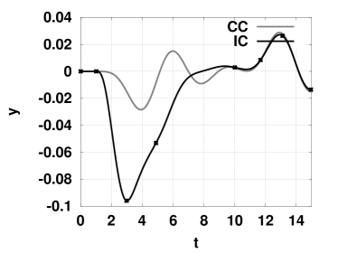
(a) $y_{1}$

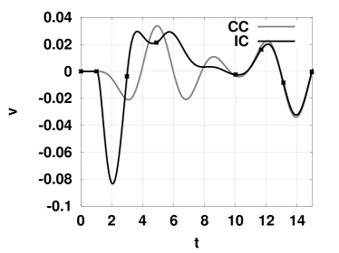
(b) $v_{1}$

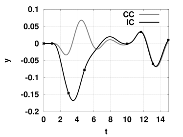
(c) $y_{2}$

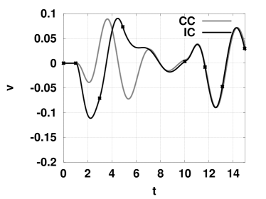
(d) $v_{2}$

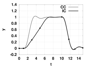
(e) $y_{3}$

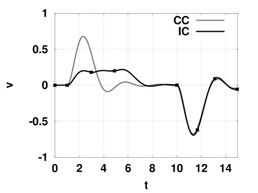
(f) $v_{3}$

Figure 15: Constrained control of mass-spring system. The left-hand column shows the positions of masses 1–3 and the right-hand column the corresponding velocities. The grey line corresponds to the simulation of the underlying unconstrained continuous system and the black lines to intermittent control; the $\bullet$ correspond to the intermittent sampling times $t_{i}$.

Figure 14 shows a coupled mass-spring system. The five masses $m_{1}$–$m_{5}$ all have unit mass and the four springs $\kappa_{1}$–$\kappa_{5}$ all have unit stiffness. The mass positions are denoted by $y_{1}$–$y_{5}$, velocities by $v_{1}$–$v_{5}$ the applied forces by $F_{1}$–$F_{5}$. In addition it is assumed that the five forces $F_{i}$ are generated from the five control signals $u_{i}$ by simple integrators thus:

$$\dot{F}_{i}=u_{i},\;i=1\dots 5$$ (6.1)

This system has fifteen states ($n_{x}=15$), five inputs ($n_{u}=5$) and five outputs ($n_{y}=5$).

To examine the effect of constraints, consider the case where it is required that the velocity of the centre mass ($i=3$) is constrained above by

$$v_{3}<0.2$$ (6.2)

but unconstrained below. As noted in Section 5.2.1, the constraints are at discrete values of intersample time $\tau$. In this case, fifty points where chosen at $\tau=0.1,0.2,\dots 5.0$. The precise choice of these points is not critical.

In addition, the system setpoint is given by

$$w_{i}(t)=\begin{cases}1&i=3\text{ and }1\leq t<10\\ 0&\text{ otherwise }\end{cases}$$ (6.3)

Figure 15 shows the results of simulating the coupled mass-spring system of Figure 14 with constrained intermittent control with constraint given by (6.2) and setpoint by (6.3). Figure 15(a) shows the position of the first mass and 15(b) the corresponding velocity; Figure 15(c) shows the position of the second mass and 15(d) the corresponding velocity; Figure 15(e) shows the position of the third mass and 15(f) the corresponding velocity. The fourth and fifth masses are not shown. In each case, the corresponding simulation result for the underlying continuous (unconstrained) simulation is also shown.

Note that on the forward motion of mass three, the velocity (Figure 15(f)) is constrained and this is reflected in the constant slope of the corresponding position (Figure 15(e)). However, the backward motion is unconstrained and closely approximates that corresponding to the unconstrained continuous controller. The other masses (which have a zero setpoint) deviate more from zero whilst mass three is constrained, but are similar to the unconstrained case when mass three is not constrained.

7 Examples: human standing

Human control strategies in the context of quiet standing have been investigated over many years by a number of authors. Early work, for example (Peterka, 2002; Lakie et al., 2003; Bottaro et al., 2005; Loram et al., 2005), was based on a single inverted pendulum, single-input model of the system. More recently, it has been shown (Pinter et al., 2008; Günther et al., 2009, 2011, 2012) that a multiple segment multiple input model is required to model unconstrained quiet standing and this clearly has implications for the corresponding human control system. Intermittent control has been suggested as the basic algorithm Gawthrop et al. (2011), Gawthrop et al. (2013b) and Gawthrop et al. (2014) and related algorithms have been analysed by Insperger (2006); Stepan and Insperger (2006), Asai et al. (2009) and Kowalczyk et al. (2012).

This section uses a linear three-segment model to illustrate key features of the contrained multivariable intermittent control described in Sections 3 and 5. Section 7.1 describes the three-link model, Section 7.2 looks at a heirachical approach to muscle-level control, Section 7.3 looks at an intermittent explanation of quiet standing and Sections 7.4 and 7.5 discuss tracking and disturbance rejection respectively.

7.1 A three-segment model

This section uses the linearised version of the three link, three joint model of posture given by Alexandrov et al. (2005). The upper, middle and lower links are indicated by subscripts $u$, $m$ and $l$ respectively. The linearised equations correspond to:

$$\mathbf{M}\ddot{\boldsymbol{\theta}}-\mathbf{G}\boldsymbol{\theta}=\mathbf{N}\mathbf{T}$$ (7.1)

where $\boldsymbol{\theta}$ is the vector of link angles given by:

$$\boldsymbol{\theta}=\begin{bmatrix}\theta_{l}\\ \theta_{m}\\ \theta_{u}\end{bmatrix}$$ (7.2)

and $\mathbf{T}$ the vector of joint torques.

the mass matrix $\mathbf{M}$ is given by

$$\mathbf{M} =b\begin{bmatrix}m_{ll}&m_{lm}&m_{lu}\\ m_{ml}&m_{mm}&m_{mu}\\ m_{ul}&m_{um}&m_{uu}\end{bmatrix}$$ (7.3)

$$\text{where }m_{ll} =m_{l}c_{l}^{2}+(m_{m}+m_{u})l_{l}^{2}+I_{l}$$ (7.4)

$$m_{mm} =m_{m}c_{m}^{2}+m_{u}l_{m}^{2}+I_{m}$$ (7.5)

$$m_{uu} =m_{u}c_{u}^{2}+I_{u}$$ (7.6)

$$m_{ml} =m_{lm}=m_{m}c_{m}l_{l}+m_{u}l_{l}l_{m}$$ (7.7)

$$m_{ul} =m_{lu}=m_{u}c_{u}l_{l}$$ (7.8)

$$m_{um} =m_{mu}=m_{u}c_{u}l_{m}$$ (7.9)

the gravity matrix $\mathbf{G}$ by

$$\mathbf{G} =g\begin{bmatrix}g_{ll}&0&0\\ 0&g_{mm}&0\\ 0&0&g_{uu}\end{bmatrix}$$ (7.10)

$$\text{where }g_{ll} =m_{l}c_{l}+(m_{m}+m_{u})l_{l}$$ (7.11)

$$g_{mm} =m_{m}c_{m}+m_{u}l_{m}$$ (7.12)

$$g_{uu} =m_{u}c_{u}$$ (7.13)

and the input matrix $\mathbf{N}$ by

$$\mathbf{N}=\begin{bmatrix}1&-1&0\\ 0&1&-1\\ 0&0&1\end{bmatrix}$$ (7.14)

The joint angles $\phi_{l}\dots\phi_{u}$ can be written in terms of the link angles as:

$$\phi_{l} =\theta_{l}$$ (7.15)

$$\phi_{m} =\theta_{m}-\theta_{l}$$ (7.16)

$$\phi_{u} =\theta_{u}-\theta_{m}$$ (7.17)

or more compactly as:

$$\boldsymbol{\phi} =\mathbf{N}^{T}\boldsymbol{\theta}$$ (7.18)

$$\text{where }\boldsymbol{\phi} =\begin{bmatrix}\phi_{l}\\ \phi_{m}\\ \phi_{u}\end{bmatrix}$$ (7.19)

The values for the link lengths $l$, CoM location $c$, masses $m$ and moments of inertia (about CoM) were taken from Figure 4.1 and Table 4.1 of Winter (2009).

The model of Equation (7.1) can be rewritten as:

$$\frac{d\mathbf{x}_{0}}{dt} =\mathbf{A}_{0}\mathbf{x}_{0}+\mathbf{B}_{0}\mathbf{T}$$ (7.20)

$$\mathbf{x}_{0} =\begin{bmatrix}\dot{\boldsymbol{\theta}}\\ \boldsymbol{\theta}\end{bmatrix}$$ (7.21)

and

$$\mathbf{A}_{0} =\begin{bmatrix}{{\mathbf{0}}}_{3\times 3}&-\mathbf{M}^{-1}\mathbf{G}\\ \mathbf{I}_{3\times 3}&{{\mathbf{0}}}_{3\times 3}\end{bmatrix}$$ (7.22)

$$\mathbf{B}_{0} =\begin{bmatrix}\mathbf{M}^{-1}\mathbf{N}\\ {{\mathbf{0}}}_{3\times 3}\end{bmatrix}$$ (7.23)

The eigenvalues of $\mathbf{A}_{0}$ are: $\pm 2.62$, $\pm 6.54$ and $\pm 20.4$. The positive eigenvalues indicate that this system is (without control) unstable.

More sophisticated models would include nonlinear geometric and damping effects; but this model provides the basi for illustating the properties of constrained intermittent control.

7.2 Muscle model & hierarchical control

As discussed by Lakie et al. (2003) and Loram et al. (2005), the single-inverted pendulum model of balance control uses a muscle model comprising a spring and a contractile element. In this context, the effect of the spring is to counteract gravity and thus effectively slow down the toppling speed on the pendulum. This toppling speed is directly related to the maximum real part of the system eigenvalues. This is important as it reduces the control bandwidth necessary to stabilise the unstable inverted pendulum system (Stein, 2003; Loram et al., 2006).

The situation is more complicated in the multiple link case as, unlike the single inverted pendulum case, the joint angles are distinct from the link angles. From Equation (7.10), the gravity matrix is diagonal in link space; on the other hand, as the muscle springs act at the joints, the corresponding stiffness matrix is diagonal in joint space and therefore cannot cancel the gravity matrix in all configurations.

The spring model used here is the multi-link extension of the model of Loram et al. (2005, Figure 1) and is given by:

$$\mathbf{T}_{k} =\mathbf{K}_{\phi}\left(\boldsymbol{\phi}_{0}-\boldsymbol{\phi}\right)$$ (7.24)

$$\text{where }\mathbf{K}_{\phi} =\begin{bmatrix}k_{1}&0&0\\ 0&k_{2}&0\\ 0&0&k_{3}\end{bmatrix}\text{and }\boldsymbol{\phi}_{0} =\begin{bmatrix}\phi_{l0}\\ \phi_{m0}\\ \phi_{u0}\end{bmatrix}$$ (7.25)

$\mathbf{T}_{k}$ is the vector of spring torques at each joint, $\boldsymbol{\phi}$ contains the joint angles (7.19) and $k_{1}\dots k_{3}$ are the spring stiffnesses at each joint. It is convenient to choose the control signal $\mathbf{u}$ to be:

$$\mathbf{u}=\frac{d\boldsymbol{\phi}_{0}}{dt}$$ (7.26)

and thus Equation (7.24) can be rewritten as:

$$\frac{d\mathbf{T}_{k}}{dt} =\mathbf{K}_{\phi}\left(\mathbf{u}-\frac{d\phi}{dt}\right)$$ (7.27)

$$=\mathbf{K}_{\phi}\left(\mathbf{u}-\mathbf{N}^{T}\frac{d\theta}{dt}\right)$$ (7.28)

Setting $\mathbf{T}=\mathbf{T}_{k}+\mathbf{T}_{d}$ where $\mathbf{T}_{d}$ is a disturbance torque, the composite system formed from the link dynamics (7.1) and the spring dynamics (7.27) is given by Equation (2.1) where:

$$\mathbf{x} =\begin{bmatrix}\mathbf{x}_{0}\\ \mathbf{T}\end{bmatrix}=\begin{bmatrix}\dot{\boldsymbol{\theta}}\\ \boldsymbol{\theta}\\ \mathbf{T}\end{bmatrix}$$ (7.29)

$$\mathbf{y} =\boldsymbol{\theta}$$ (7.30)

$$\mathbf{d} =\mathbf{T}_{d}$$ (7.31)

and

$$\mathbf{A} =\begin{bmatrix}\mathbf{A}_{0}&\mathbf{B}_{0}\\ -\mathbf{K}_{\phi}\mathbf{N}^{T}&{{\mathbf{0}}}_{3\times 6}\end{bmatrix}=\begin{bmatrix}{{\mathbf{0}}}_{3\times 3}&-\mathbf{M}^{-1}\mathbf{G}&\mathbf{M}^{-1}\mathbf{N}\\ \mathbf{I}_{3\times 3}&{{\mathbf{0}}}_{3\times 3}&{{\mathbf{0}}}_{3\times 3}\\ -\mathbf{K}_{\phi}\mathbf{N}^{T}&{{\mathbf{0}}}_{3\times 3}&{{\mathbf{0}}}_{3\times 3}\end{bmatrix}$$ (7.32)

$$\mathbf{B} =\begin{bmatrix}{{\mathbf{0}}}_{3\times 3}\\ {{\mathbf{0}}}_{3\times 3}\\ \mathbf{K}_{\phi}\end{bmatrix}$$ (7.33)

$$\mathbf{B}_{d} =\begin{bmatrix}\mathbf{B}_{0}\\ {{\mathbf{0}}}_{3\times 3}\end{bmatrix}=\begin{bmatrix}\mathbf{M}^{-1}\mathbf{N}\\ {{\mathbf{0}}}_{3\times 3}\\ {{\mathbf{0}}}_{3\times 3}\end{bmatrix}$$ (7.34)

$$\mathbf{C} =\begin{bmatrix}{{\mathbf{0}}}_{3\times 3}&\mathbf{I}_{3\times 3}&{{\mathbf{0}}}_{3\times 3}\end{bmatrix}$$ (7.35)

There are, of course, many other state-space representations with the same input-output properties, but this particular state space representation has two useful features: firstly, the velocity control input of Equation (7.26) induces an integrator in each of the three inputs and secondly the state explicitly contains the joint torque due to the springs. The former feature simplifies control design in the presence of input disturbances with constant components and the latter feature allows spring preloading (in anticipation of a disturbance) to be modelled as a state initial condition. These features are used in the example of Section 7.5.

(a) Real parts

(b) Imaginary parts

(c) Spring constants $\mathbf{k}_{\phi}$

Figure 16: Choosing the spring constants. (a) The real parts of the non-zero eigenvalues plotted against $\sigma_{max}$, the specified maximum real part of all eigenvalues resulting from (7.37) & (7.38). (b) The imaginary parts corresponding to (a). (c) The spring constants $\mathbf{k}_{\phi}$.

It has been argued (Hogan, 1984) that humans use muscle co-activation of antagonist muscles to manipulate the passive muscle stiffness and thus $\mathbf{K}_{\phi}$. As mentioned above, the choice of $\mathbf{K}_{\phi}$ in the single-link case (Loram et al., 2005, Figure 1) directly affects the toppling speed via the maximum real part of the system eigenvalues. Hence we argue that such muscle co-activation could be used to choose the maximum real part of the system eigenvalues and thus manipulate the required closed-loop control bandwidth. However, muscle co-activation requires the flow of energy and so it makes sense to choose the minimal stiffness consistent with the required maximum real part of the system eigenvalues. Defining:

$$\mathbf{k}_{phi}=\begin{bmatrix}k_{1}\\ k_{2}\\ k_{3}\end{bmatrix}$$ (7.36)

this can be expressed mathematically as:

$$\min_{\mathbf{k}_{\phi}}||\mathbf{K}_{\phi}||$$ (7.37)

$$\text{subject to }\max\left[\Re\sigma_{i}\right]<\sigma_{max}$$ (7.38)

where $\sigma_{i}$ is the $i$th eigenvalue of $\mathbf{A}$. This is a quadratic optimisation with non-linear constraints which can be solved by sequential quadratic programming (SQP) (Fletcher, 1987).

In the single-link case, increasing spring stiffness from zero decreases the value of the positive eigenvalue until it reaches zero, after that point the two eigenvalues form a complex-conjugate pair with zero real part. The three link case corresponds to three eigenvalue pairs. Figure 16 shows how the real and imaginary parts of these six eigenvalues vary with the constraint $\sigma_{max}$ together with the spring constants $\mathbf{k}_{\phi}$. Note that the spring constants and imaginary parts rise rapidly when the maximum real eigenvalue is reduced to below about 2.3.

Joint damping can be modelled by the equation:

$$\mathbf{T}_{c} =-\mathbf{C}_{\phi}\frac{d\boldsymbol{\phi}}{dt}=-\mathbf{C}_{\phi}\mathbf{N}^{T}\frac{d\boldsymbol{\theta}}{dt}$$ (7.39)

$$\text{where }\mathbf{C}_{\phi} =\begin{bmatrix}c_{1}&0&0\\ 0&c_{2}&0\\ 0&0&c_{3}\end{bmatrix}$$ (7.40)

Setting $\mathbf{T}=\mathbf{T}_{k}+\mathbf{T}_{c}$ the matrix $\mathbf{A}$ of Equation (7.32) is replaced by:

$$\mathbf{A} =\begin{bmatrix}-\mathbf{M}^{-1}\mathbf{N}\mathbf{C}_{\phi}\mathbf{N}^{T}&-\mathbf{M}^{-1}\mathbf{G}&\mathbf{M}^{-1}\mathbf{N}\\ \mathbf{I}_{3\times 3}&{{\mathbf{0}}}_{3\times 3}&{{\mathbf{0}}}_{3\times 3}\\ -\mathbf{K}_{\phi}\mathbf{N}^{T}&{{\mathbf{0}}}_{3\times 3}&{{\mathbf{0}}}_{3\times 3}\end{bmatrix}$$ (7.41)

7.3 Quiet standing

(a) $q_{t}=0^{\circ}$: $\theta_{l}^{\circ}$

(b) $q_{t}=0^{\circ}$: $\theta_{m}^{\circ}$

(c) $q_{t}=0^{\circ}$: $\theta_{u}^{\circ}$

(d) $q_{t}=0.1^{\circ}$: $\theta_{l}^{\circ}$

(e) $q_{t}=0.1^{\circ}$: $\theta_{m}^{\circ}$

(f) $q_{t}=0.1^{\circ}$: $\theta_{u}^{\circ}$

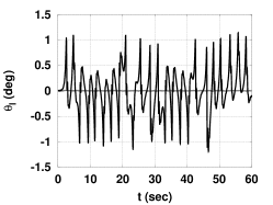
(g) $q_{t}=1^{\circ}$: $\theta_{l}^{\circ}$

(h) $q_{t}=1^{\circ}$: $\theta_{m}^{\circ}$

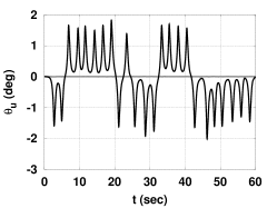
(i) $q_{t}=1^{\circ}$: $\theta_{u}^{\circ}$

Figure 17: Quiet standing with torque disturbance at the lower joint. Each row shows the lower ($\boldsymbol{\theta}_{l}$), middle ($\boldsymbol{\theta}_{m}$) and upper ($\boldsymbol{\theta}_{u}$) link angles (deg) plotted against time $t$ (sec) for a different thresholds $q_{t}$. Larger thresholds give larger, and more regular sway angles.

(a) $q_{t}=0^{\circ}$: $\theta_{l}^{\circ}$

(b) $q_{t}=0^{\circ}$: $\theta_{m}^{\circ}$

(c) $q_{t}=0^{\circ}$: $\theta_{u}^{\circ}$

(d) $q_{t}=0.1^{\circ}$: $\theta_{l}^{\circ}$

(e) $q_{t}=0.1^{\circ}$: $\theta_{m}^{\circ}$

(f) $q_{t}=0.1^{\circ}$: $\theta_{u}^{\circ}$

(g) $q_{t}=1^{\circ}$: $\theta_{l}^{\circ}$

(h) $q_{t}=1^{\circ}$: $\theta_{m}^{\circ}$

(i) $q_{t}=1^{\circ}$: $\theta_{u}^{\circ}$

Figure 18: Quiet standing: phase-plane. Each plot corresponds to that of Figure 17 but the angular velocity is plotted against angle. Again, the increase in sway angle and angular velocity with threshold is evident.

In the case of quiet standing, there is no setpoint tracking and no constant disturbance and thus $w=0$ and $\mathbf{x}_{ss}$ is not computed. The spring constants were computed as in Section 7.2 with $\sigma_{max}=3$. The corresponding non-zero eigenvalues of $\mathbf{A}$ are $\pm 3$, $\pm 2.38$, $\pm j17.9$ The intermittent controller of Section 3, based on the continuous-time controller of Section 2.3 was simulated using the following control design parameters:

$$\mathbf{Q}_{c} =\begin{bmatrix}q_{v}\mathbf{I}_{3\times 3}&{{\mathbf{0}}}_{3\times 3}&{{\mathbf{0}}}_{3\times 3}\\ {{\mathbf{0}}}_{3\times 3}&q_{p}\mathbf{I}_{3\times 3}&{{\mathbf{0}}}_{3\times 3}\\ {{\mathbf{0}}}_{3\times 3}&{{\mathbf{0}}}_{3\times 3}&q_{\mathbf{T}}\mathbf{I}_{3\times 3}\end{bmatrix}$$ (7.42)

$$\text{where }q_{v} =0,\;q_{p}=1,\;q_{\mathbf{T}}=10$$ (7.43)

$$\mathbf{R}_{c} =\mathbf{K}_{phi}^{2}$$ (7.44)

The corresponding closed-loop poles are $-3.45\pm 18.3$, $-3.95\pm 3.82$, $-2.87\pm 0.590$, $-5.31$, $-3.28$ and $-2.48$. The intermittent control parameters (Section 3) were time delay $\Delta$ and minimum intermittent interval $\Delta_{min}$ were chosen as:

$$\Delta =0.1\text{s}$$ (7.45)

$$\Delta_{min} =0.25\text{s}$$ (7.46)

These parameters are used in all of the following simulations.

A multisine disturbance with standard deviation $0.01\text{Nm}$ was added to the control signal at the lower (ankle) joint. With reference to Equation (3.20), the threshold was set on the three segment angles so that the threshold surface (in the 9D state-space) was defined as:

$$\boldsymbol{\theta}^{T}\boldsymbol{\theta} =\mathbf{x}^{T}\mathbf{Q}_{t}\mathbf{x}=q_{t}^{2}$$ (7.47)

$$\text{where }\mathbf{Q}_{t}\ =\begin{bmatrix}{{\mathbf{0}}}_{3\times 3}&{{\mathbf{0}}}_{3\times 3}&{{\mathbf{0}}}_{3\times 3}\\ {{\mathbf{0}}}_{3\times 3}&\mathbf{I}_{3\times 3}&{{\mathbf{0}}}_{3\times 3}\\ {{\mathbf{0}}}_{3\times 3}&{{\mathbf{0}}}_{3\times 3}&{{\mathbf{0}}}_{3\times 3}\end{bmatrix}$$ (7.48)

Three simulations of both IC and CC were performed with event threshold $q_{t}=0^{\circ}$, $q_{t}=0.1^{\circ}$ and $q_{t}=1^{\circ}$ and the resultant link angles $\boldsymbol{\theta}$ are plotted against time in Figure 17; the black lines show the IC simulations and the grey lines the CC simulations. The three-segment model together with the spring model has 9 states. Figure 18 shows three cross sections though this space (by plotting segment angular velocity against segment angle) for the three thresholds.

As expected, the small threshold gives smaller displacements from vertical; but the disturbance is more apparent. The large threshold gives largely self-driven behaviour. This behaviour is discussed in more detail by Gawthrop et al. (2014).

7.4 Tracking

(a) $\theta_{u}=0^{\circ}$, $\phi_{m}=0^{\circ}$

(b) $\theta_{u}=0^{\circ}$, $\phi_{m}=-10^{\circ}$

(c) $\theta_{u}=0^{\circ}$, $\phi_{m}=-20^{\circ}$

(d) $\theta_{u}=10^{\circ}$, $\phi_{m}=0^{\circ}$

(e) $\theta_{u}=10^{\circ}$, $\phi_{m}=-10^{\circ}$

(f) $\theta_{u}=10^{\circ}$, $\phi_{m}=-20^{\circ}$

Figure 19: Equilibria: Link Configuration. (a),(b),(c). In each configuration, the upper link is set at $\theta_{u}=0^{\circ}$ and the posture is balanced (no ankle torque); the knee angle is set to three possible values. (d),(e),(f) as (a),(b),(c) but $\theta_{u}=10^{\circ}$

(a) Link angles

(b) Joint angles

(c) Joint torques

Figure 20: Equilibria: angles and torques. (a) The equilibrium link angles $\boldsymbol{\theta}$ are plotted against the fixed knee angle $\phi_{m}$ with balanced posture and the upper link at an angle of $\theta_{u}=10^{\circ}$. (b) & (c) As (a) but with joint angles $\boldsymbol{\phi}$ and joint torques $\mathbf{T}$ respectively. Note that the ankle torque $T_{l}$ is zero (balanced posture) and the waist torque $T_{u}$ balances the fixed $\theta_{u}=10^{\circ}$.

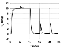
(a) $q_{t}=0^{\circ}$: $\theta_{u}^{\circ}$

(b) $q_{t}=0^{\circ}$: $\phi_{m}^{\circ}$

(c) $q_{t}=0^{\circ}$: $g_{l}^{\circ}$

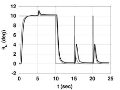
(d) $q_{t}=0.1^{\circ}$: $\theta_{u}^{\circ}$

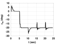
(e) $q_{t}=0.1^{\circ}$: $\phi_{m}^{\circ}$

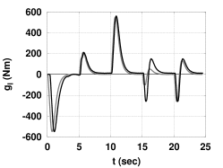
(f) $q_{t}=0.1^{\circ}$: $g_{l}^{\circ}$

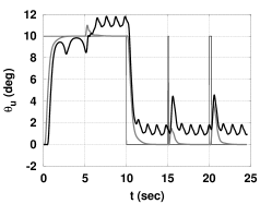
(g) $q_{t}=1^{\circ}$: $\theta_{u}^{\circ}$

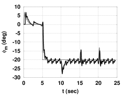
(h) $q_{t}=1^{\circ}$: $\phi_{m}^{\circ}$

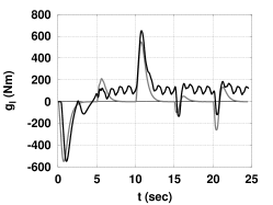
(i) $q_{t}=1^{\circ}$: $g_{l}^{\circ}$

Figure 21: Tracking: controlled knee joint. The equilibrium design (Section 2.4) sets the upper link angle $\boldsymbol{\theta}_{u}$ to $10^{\circ}$ for $t<10$ and to to $0^{\circ}$ for $10\leq t<15$ and sets the gravity torque at the ankle joint to zero; it also sets the knee angle $\phi_{m}$ to zero for $t<5$ and to $-20^{\circ}$ for $t\geq 5$. At time $t=15$ a pulse of width 0.1s is applied to the upper link angle setpoint and a a pulse of width 0.25s is applied at time $t=20$. Note that the intermittent control response is similar in each case: this refractory behaviour is due to event-driven control with a minimum intermittent interval $\Delta_{min}=0.25$ (7.46).

(a) $q_{t}=0^{\circ}$: $\theta_{u}^{\circ}$

(b) $q_{t}=0^{\circ}$: $\phi_{m}^{\circ}$

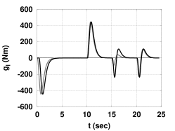
(c) $q_{t}=0^{\circ}$: $g_{l}^{\circ}$

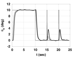
(d) $q_{t}=0.1^{\circ}$: $\theta_{u}^{\circ}$

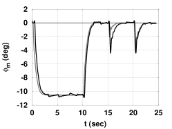
(e) $q_{t}=0.1^{\circ}$: $\phi_{m}^{\circ}$

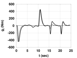
(f) $q_{t}=0.1^{\circ}$: $g_{l}^{\circ}$

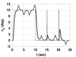
(g) $q_{t}=1^{\circ}$: $\theta_{u}^{\circ}$

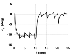
(h) $q_{t}=1^{\circ}$: $\phi_{m}^{\circ}$

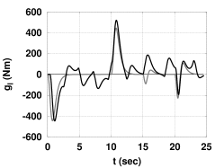
(i) $q_{t}=1^{\circ}$: $g_{l}^{\circ}$

Figure 22: Tracking: free knee joint. This Figure corresponds to Figure 21 except that the knee joint angle $\phi_{m}$ is not constrained.

As discussed in Section 2.4, the equilibrium state $\mathbf{x}_{ss}$ has to be designed for tracking purposes. As there are three inputs, it is possible to satisfy up to three steady-state conditions. Three possible steady-state conditions are:

1. The upper link should follow a setpoint:

   $$\boldsymbol{\theta}_{u}=w_{u}$$ (7.49)

2. The the component of ankle torque due to gravity should be zero:

   $$\mathbf{T}_{1}=\begin{bmatrix}1&0&0\end{bmatrix}\mathbf{N}^{-1}\mathbf{G}\boldsymbol{\theta}=0$$ (7.50)

3. The knee angle should follow a set point:

   $$\phi_{m}=\theta_{m}-\theta_{l}=w_{m}$$ (7.51)

These conditions correspond to:

$$\mathbf{C}_{ss} =\begin{bmatrix}0&0&0&0&0&1&0&0&0\\ 0&0&0&27.14627&22.51155&23.74238&0&0&0\\ 0&0&0&-1&1&0&0&0&0\end{bmatrix}$$ (7.52)

$$\mathbf{y}_{ss} =\mathbf{I}_{3\times 3}$$ (7.53)

$$\mathbf{w}(t) =\begin{bmatrix}w_{u}(t)\\ 0\\ w_{m}(t)\end{bmatrix}$$ (7.54)

This choice is examined in Figures 19 and 20 by choosing the knee angle $\phi_{m}=\theta_{m}-\theta_{l}$. Figure 20 shows how the link and joint angles, and the corresponding torques, vary with $\phi_{m}$. Figure 19 shows a picture of the three links for three values of $\phi_{m}$. In each case, note that the upper link and the corresponding hip torque remain constant due to the first condition and that each configuration appears balanced due to condition 2.

The simulations shown in Figure 21 shows the tracking of a setpoint $\mathbf{w}(t)$ (7.54) using the three conditions for determining the steady-state. In this example, the individual setpoint components of Equation (7.54) are:

$$w_{u}(t) =\begin{cases}10^{\circ}&0<t\leq 10\\ 0^{\circ}&10<t\leq 15\\ 0^{\circ}&10<t\leq 15\\ 10^{\circ}&15<t\leq 15.1\\ 0^{\circ}&15.1<t\leq 20\\ 10^{\circ}&20<t\leq 20.25\\ 0^{\circ}&t>20.25\end{cases}$$ (7.55)

$$w_{m}(t) =\begin{cases}0^{\circ}&0<t\leq 5\\ -20^{\circ}&t>5\end{cases}$$ (7.56)

As a further example, only the first two conditions for determining the steady-state are used; the knee is not included. These conditions correspond to:

$$\mathbf{C}_{ss} =\begin{bmatrix}0&0&0&0&0&1&0&0&0\\ 0&0&0&27.14627&22.51155&23.74238&0&0&0\end{bmatrix}$$ (7.57)

$$\mathbf{y}_{ss} =\mathbf{I}_{2\times 2}$$ (7.58)

$$\mathbf{w}(t) =\begin{bmatrix}w_{u}(t)\\ 0\end{bmatrix}$$ (7.59)

The under-determined equation (2.13) is solved using the pseudo inverse. The simulations shown in Figure 22 shows the tracking of a setpoint $\mathbf{w}(t)$ (7.54) using the first two conditions for determining the steady-state. In this example, the individual setpoint component $w_{u}$ is given by (7.55). Comparing Figure 22(b), (e) & (h) with Figure 21(b), (e) & (h), it can be seen that the knee angle is no longer explicitly controlled.

7.5 Disturbance rejection

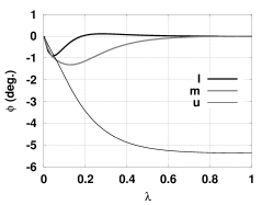
(a) Joint angle $\phi$ (deg) – unconstrained

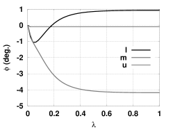
(b) Joint angle $\phi$ (deg) – constrained

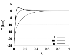
(c) Joint torque $\mathbf{T}$ (nm) – unconstrained

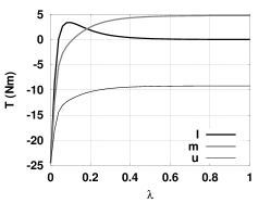
(d) Joint torque $\mathbf{T}$ (nm) – constrained

Figure 23: Equilibria. For a constant disturbance torque $\mathbf{T}_{d}$ acting on the upper link, the plots show how link angle and joint torque vary with the weighting factor $\lambda$. $\lambda=0$ gives an upright posture (zero link and joint angles – Figure 24(a)) and $\lambda=1$ gives a balanced posture (zero joint torques – Figure 24(e)). $\lambda=0.5$ gives an intermediate posture (Figure 24(c)). The left column is the unconstrained case, the right column is the constrained case where hip angle $\phi_{u}>-0.1^{\circ}$ and knee angle $\phi_{m}<0$; the former constraint becomes active as $\lambda$ increases and the knee and hip joint torques are no longer zero at $\lambda=1$.

(a) Upright ($\lambda=0$) – unconstrained

(b) Upright ($\lambda=0$) – constrained

(c) Intermediate ($\lambda=0.5$) – unconstrained

(d) Intermediate ($\lambda=0.5$) – constrained

(e) Balanced ($\lambda=1$) – unconstrained

(f) Balanced ($\lambda=1$) – constrained

Figure 24: Equilibria: link configurations. (a),(c),(e) unconstrained; (b),(d),(f) constrained where hip angle $\phi_{u}>-0.1^{\circ}$ and knee angle $\phi_{m}<0$.

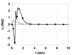
(a) Lower joint: angle $\theta_{l}$ (deg)

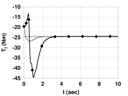
(b) Lower joint: torque $T_{l}$ (nm)

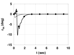
(c) Middle joint: angle $\theta_{m}$ (deg)

(d) Middle joint: torque $T_{m}$ (nm)

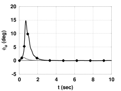
(e) Upper joint: angle $\theta_{u}$ (deg)

(f) Upper joint: torque $T_{u}$ (nm)

Figure 25: Pole-lifting simulation – constrained: upright posture ($\lambda=0$). The spring preload $\kappa$ (7.63) is 80%. Note that the steady state link angles are zero and the steady-state torques are all $-T_{d}$ to balance $T_{d}=gm_{p}l_{p}=24.5$Nm (7.60). The dots correspond to the sample times $t_{i}$. The intervals $\Delta_{i}$ (3.1) are irregular and greater than the minimum $\Delta_{min}$.

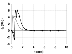
(a) Lower joint: angle $\theta_{l}$ (deg)

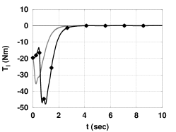
(b) Lower joint: torque $T_{l}$ (nm)

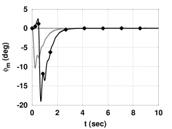
(c) Middle joint: angle $\theta_{m}$ (deg)

(d) Middle joint: torque $T_{m}$ (nm)

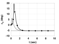
(e) Upper joint: angle $\theta_{u}$ (deg)

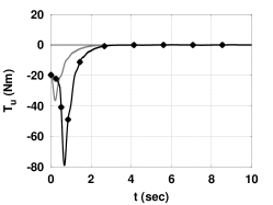
(f) Upper joint: torque $T_{u}$ (nm)

Figure 26: Pole-lifting simulation – unconstrained steady-state: balanced posture ($\lambda=1$). The spring preload $\kappa$ (7.63) is 80%. The steady state joint torques are zero.

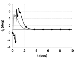
(a) Lower joint: angle $\theta_{l}$ (deg)

(b) Lower joint: torque $T_{l}$ (nm)

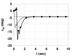
(c) Middle joint: angle $\theta_{m}$ (deg)

(d) Middle joint: torque $T_{m}$ (nm)

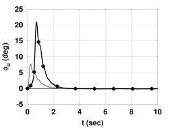
(e) Upper joint: angle $\theta_{u}$ (deg)

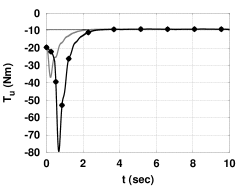
(f) Upper joint: torque $T_{u}$ (nm)

Figure 27: Pole-lifting simulation – constrained steady-state: balanced posture ($\lambda=1$). The spring preload $\kappa$ (7.63) is 80%. Due to the constraints, the steady state joint torques $\mathbf{T}_{u}$ and $\mathbf{T}_{m}$ are not zero, but the upper (hip) joint is now constrained.

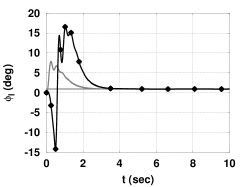
(a) Lower joint: angle $\theta_{l}$ (deg)

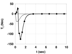
(b) Lower joint: torque $T_{l}$ (nm)

(c) Middle joint: angle $\theta_{m}$ (deg)

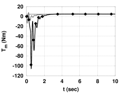
(d) Middle joint: torque $T_{m}$ (nm)

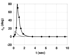
(e) Upper joint: angle $\theta_{u}$ (deg)

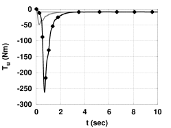
(f) Upper joint: torque $T_{u}$ (nm)

Figure 28: Pole-lifting simulation – constrained steady-state but with 0% preload. This is the same as Figure 27 except that the spring preload is 0%.

Detailed modelling of a human lifting and holding a heavy pole would require complicated dynamical equations. This section looks at a simple approximation to the case where a heavy pole of mass $m_{p}$ is held at a fixed distance $l_{p}$ to the the body. In particular, the effect is modelled by

1. adding a torque disturbance $T_{d}$ to the upper link where

   $$T_{d}=gm_{p}l_{p}$$ (7.60)

2. adding a mass $m_{p}$ to the upper link.

In terms of the system Equation (2.1) and the three link model of Equation (7.1), the disturbance $\mathbf{d}$ is given by

$$\mathbf{d} =N^{-1}\begin{bmatrix}0\\ 0\\ T_{d}\end{bmatrix}$$ (7.61)

$$=\begin{bmatrix}1\\ 1\\ 1\end{bmatrix}T_{d}$$ (7.62)

As discussed in Section 7.2, it is possible to preload the joint spring to give an initial torque. In this context, this is done by initialising the system state $\mathbf{x}$ of Equation (7.29) as:

$$\mathbf{x}(0)=\begin{bmatrix}\dot{\boldsymbol{\theta}}(0)\\ \boldsymbol{\theta}(0)\\ \mathbf{T}(0)\end{bmatrix}=\begin{bmatrix}{{\mathbf{0}}}_{3\times 1}\\ {{\mathbf{0}}}_{3\times 1}\\ \kappa\mathbf{d}\end{bmatrix}$$ (7.63)

$\kappa$ will be referred to as the spring preload and will be expressed as a percentage: thus $\kappa=0.8$ will be referred to as 80% preload.

There are many postures appropriate to this situation, two of which are:

upright

: all joint angles are zero and the pole is balanced by appropriate joint torques (Figures 24(a) & 24(b));

balanced

: all joint torques are zero and the pole is balanced by appropriate joint (and thus link) angles (Figures 24(e) & 24(f)).

In terms of Equation (2.12), the upright posture is specified by choosing:

$$\mathbf{C}_{ss} =\begin{bmatrix}{{\mathbf{0}}}_{3\times 3}&\mathbf{I}_{3\times 3}&{{\mathbf{0}}}_{3\times 3}\end{bmatrix}$$ (7.64)

$$\mathbf{y}_{ss} ={{\mathbf{0}}}_{3\times 1}$$ (7.65)

and the balanced posture is specified by choosing:

$$\mathbf{C}_{ss} =\begin{bmatrix}{{\mathbf{0}}}_{3\times 3}&{{\mathbf{0}}}_{3\times 3}&\mathbf{I}_{3\times 3}\end{bmatrix}$$ (7.66)

$$\mathbf{y}_{ss} ={{\mathbf{0}}}_{3\times 1}$$ (7.67)

A combination of both can be specified by choosing:

$$\mathbf{C}_{ss} =\begin{bmatrix}{{\mathbf{0}}}_{3\times 3}&\mathbf{I}_{3\times 3}&{{\mathbf{0}}}_{3\times 3}\\ {{\mathbf{0}}}_{3\times 3}&{{\mathbf{0}}}_{3\times 3}&\mathbf{I}_{3\times 3}\end{bmatrix}$$ (7.68)

$$\mathbf{y}_{ss} ={{\mathbf{0}}}_{6\times 1}$$ (7.69)

$$\mathbf{Q}_{ss} =\begin{bmatrix}(1-\lambda)\mathbf{I}_{3\times 3}&{{\mathbf{0}}}_{3\times 3}\\ {{\mathbf{0}}}_{3\times 3}&\frac{\lambda}{\mathbf{T}_{d}}\mathbf{I}_{3\times 3}\end{bmatrix}$$ (7.70)

The parameter $0\leq\lambda\leq 1$ weights the two postures and division by $\mathbf{T}_{d}$ renders the equations dimensionless.

When $\mathbf{C}_{ss}$ is given by (7.68), $n_{ss}=6$. As $n_{u}=3$, $n_{ss}>n_{u}$ and so, as discussed in Section 2.4, the set of equations (2.13) is over determined and the approach of Section 5 is used. Two situations are examined: unconstrained and constrained with hip angle and knee angle subject to the inequality constraints:

$$\phi_{u} >-0.1^{\circ}$$ (7.71)

$$\phi_{m} <0$$ (7.72)

In each case, the equality constraint (5.8) is imposed. Figure 23 shows how the equilibrium joint angle $\boldsymbol{\phi}$ and torque $\mathbf{T}$ vary with $\lambda$ for the two cases. As illustrated in Figure 24 the two extreme cases $\lambda=0$ and $\lambda=1$ correspond to the upright and balanced postures; other values give intermediate postures.

Figures 25 and 27 show simulation results for the two extreme cases of $\lambda$ for the unconstrained case with $m_{p}=5$kg and $l_{p}=0.5$m. In each case, the initial link angles are all zero ($\boldsymbol{\theta}_{l}=\boldsymbol{\theta}_{m}=\boldsymbol{\theta}_{u}=0$) and the disturbance torque $\mathbf{T}_{d}=g$ is applied at $t=0$. Apart from the equilibrium vector $\mathbf{x}_{ss}$, the control parameters are the same in each case.

In the case of Figure 25, the steady-state torques are $\mathbf{T}_{l}=\mathbf{T}_{m}=\mathbf{T}_{u}=-\mathbf{T}_{d}$ to balance $\mathbf{T}_{d}=gm_{p}l_{p}$; in the case of Figure 27, the links balance the applied torque by setting $\boldsymbol{\theta}_{l}=\boldsymbol{\theta}_{m}=0$ and $\boldsymbol{\theta}_{u}=\dfrac{-\Delta}{gc_{u}m_{u}}$.

8 Intermittency induces Variability

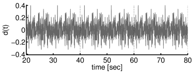
(a) Disturbance signal

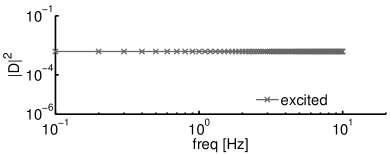
(b) Disturbance signal

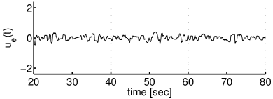
(c) Control signal (cc)

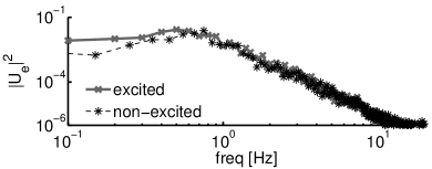
(d) Control signal (cc)

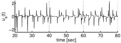
(e) Control signal (mi)

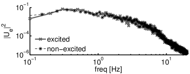
(f) Control signal (mi)

Figure 29: Experimental data showing variability during human motor control. Plots on the left side show time-domain signals, plots on the right side depict the corresponding frequency domain signals. “cc” – keep close to centre (position control), “mi” – minimal intervention (minimise control).

Variability is an important characteristic of human motor control: when repeatedly exposed to identical excitation, the response of the human operator is different for each repetition. This is illustrated in Figure 29: Figure 29(a) shows a periodic input disturbance (periodicity 10s), while Figures 29(c) and 29(e) show the corresponding output signal of a human controller for different control aims. It is clear that in both cases, the control signal is different for each 10s period of identical disturbance.

In the frequency domain, variability is represented by the observation that, when the system is excited at a range of discrete frequencies (as shown in Figure 29(b), the disturbance signal contains frequency components at $[0.1,\,0.2,\dots,10]$Hz), the output response contains information at both the excited and the non-excited frequencies (Figures 29(d) and 29(f)). The response at the non-excited frequencies (at which the excitation signal is zero) is termed the remnant.

Variability is usually explained by appropriately constructed motor- and observation noise which is added to a linear continuous-time model of the human controller (signals $v_{u}$ and $v_{y}$ in Figure 1) (Levison et al., 1969; Kleinman et al., 1970). While this is currently the prominent model in human control, its physiological basis is not fully established. This has led to the idea that the remnant signal might be based on structure rather than randomness (Newell et al., 2006).

Intermittent control includes a sampling process, which is generally based on thresholds associated with a trigger (see Figure 2). This non-uniform sampling process leads to a time-varying response of the controller. It has been suggested that the remnant can be explained by event-driven intermittent control without the need for added noise (Mamma et al., 2011; Gawthrop et al., 2013a), and that this sampling process introduces variability (Gawthrop et al., 2013b).

In this section we will discuss how intermittency can provide an explanation for variability which is based on the controller structure and does not require a random process. Experimental data from a visual-manual control task will be used as an illustrative example.

8.1 Experimental setup

In this section, experimental data from a visual-manual control task are used in which the participant were asked to use a sensitive, contactless, uniaxial joystick to sustain control of an unstable 2nd order system whose output was displayed as a dot on a oscilloscope (Loram et al., 2011). The controlled system represented an inverted pendulum with a dynamic response similar to that of a human standing (Load 2 of Table 1 in (Loram et al., 2009)),

$$\begin{cases}\frac{d{\mathbf{x}}}{dt}(t)&=\left[\begin{array}[]{c c}-0.0372&1.231\\ 1&0\end{array}\right]{\mathbf{x}}(t)+\left[\begin{array}[]{c}6.977\\ 0\end{array}\right](\mathbf{u}(t)-{\mathbf{d}^{\prime}}(t))\\ \mathbf{y}(t)&=\left[\begin{array}[]{c c}0&1\end{array}\right]{\mathbf{x}}(t)\\ \mathbf{y}_{o}(t)&=\left[\begin{array}[]{c c}1&1\end{array}\right]{\mathbf{x}}(t)\end{cases}$$ (8.1)

The external disturbance signal, $d(t)$, applied to the load input, was a multi-sine consisting of $N_{f}=100$ discrete frequencies $\omega_{k}$, with resolution $\omega_{0}=2\pi f_{0}$, $f_{0}=0.1\text{Hz}$ (Pintelon and Schoukens, 2001)

$$d(t)=\sum_{k=1}^{N_{f}}a_{k}\,cos\left(\omega_{k}t+\phi_{k}\right)\qquad\text{with}\;\omega_{k}=2\pi\,kf_{0}$$ (8.2)

The signal $d(t)$ is periodic with $T_{0}=1/f_{0}=10\text{s}$. To obtain an unpredictable excitation, the phases $\phi_{k}$ are random values taken from a uniform distribution on the open interval $(0,2\pi)$, while $a_{k}=1$ for all $k$ to ensure that all frequency are equally excited.

We considered two control priorities using the instructions “keep the dot as close to the centre as possible” (“cc”, prioritising position), and “while keeping the dot on screen, wait as long as possible before intervening” (“mi”, minimising intervention).

8.2 Identification of the linear time-invariable (LTI) response

Using previously established methods discussed in Section 9 and by Gollee et al. (2012), the design parameters (i.e. LQ design weightings and mean time-delay, $\Delta$) for an optimal, continuous-time linear predictive controller (PC) (Figure 1) are identified by fitting the complex frequency response function relating $d$ to $u_{e}$ at the excited frequencies. The linear fit to the experimental data is shown in Figures 30(a) and 30(b) for the two different experimental instructions (“cc” and “mi”). Note that the PC only fits the excited frequency components; its response at the non-excited frequencies (bottom plots) is zero.

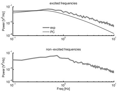
(a) Control signal (instruction “cc”)

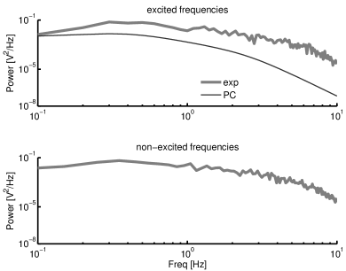
(b) Control signal (instruction “ol”)

Figure 30: Example individual result for identification of LTI response for two experimental instructions. The continuous predictive controller can fit the excited frequencies (top graphs), but can not explain the experimental response at non-excited frequencies (bottom graphs).

8.3 Identification of the remnant response

The controller design parameters (i.e. the LQ design weightings) obtained when fitting the LTI response, are used as the basis to model the response at the non-excited (remnant) frequencies. First, the standard approach of adding noise to a continuous PC is demonstrated. Following this, it is shown that event driven IC can approximate the experimental remnant response, by adjusting the threshold parameters associated with the event trigger.

8.3.1 Variability by adding noise

For the PC, noise can be injected either as observation noise, $v_{y}$, or as noise added to the input, $v_{u}$. The noise spectrum is obtained by considering the measured response $u_{e}$ at non-excited frequencies and, using the corresponding loop transfer function (see Section 9.1.1), calculating the noise input ($v_{u}$ or $v_{y}$) required to generate this. The calculated noise signal is then interpolated at the excited frequencies.

Results for added input noise ($v_{u}$) are shown in Figure 31. As expected, the fit at the non-excited frequencies is nearly perfect (Figures 31(a) and 31(b), bottom panels). Notably, the added input noise also improves the fit at the excited frequencies (Figures 31(a) and 31(b), top panels).

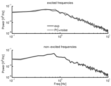
(a) Control signal (instruction “cc”)

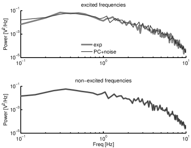
(b) Control signal (instruction “mi”)

(c) Added input noise $v_{u}$ (instruction “cc”)

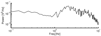
(d) Added input noise $v_{u}$ (instruction “mi”)

Figure 31: Variability as a result of coloured input noise added to a predictive continuous controller. The top graphs show the resulting fit to experimental data at excited and non-excited frequencies. The bottom graphs show the input noise added.

The spectra of the input noise $v_{u}$ are shown in Figures 31(c) and 31(d). It can be observed that the noise spectra are dependent on the instructions given (“cc” or “mi”), with no obvious physiological basis to explain this difference.

8.3.2 Variability by intermittency

As an alternative explanation, a noise-free event driven intermittent controller is considered (cf. Figure 2). The same design parameters as for the PC are used, with the time-delay set to a minimal value of $\Delta^{min}=0.1$sec and a corresponding minimal intermittent interval, $\Delta^{\text{min}}_{ol}=0.1$sec.

Variations in the loop-delay are now the result of the event thresholds, cf. equation (3.20). In particular, we consider the first two elements of the state prediction error $e_{hp}$, corresponding to the velocity ($e_{hp}^{v}$) and position ($e_{hp}^{p}$) states, and define an ellipsoidal event detection surface given by

$$\left(\frac{e_{hp}^{p}}{\theta^{p}}\right)^{2}+\left(\frac{e_{hp}^{v}}{\theta^{v}}\right)^{2}>1$$ (8.3)

where $\theta^{p}$ and $\theta^{v}$ are the thresholds associated with the corresponding states.

To find the threshold values which resulted in simulation which best approximates the experimental remnant, both thresholds were varied between 0 (corresponding to clock-driven IC) and 3, and the threshold combination that resulted in the best least-squares fit at all frequencies (excited and non-excited) was selected as the optimum. The resulting fit is shown in Figures 32(a) and 32(b). For both instructions, the event driven IC can both, explain the remnant signal and improve the fit at excited frequencies.

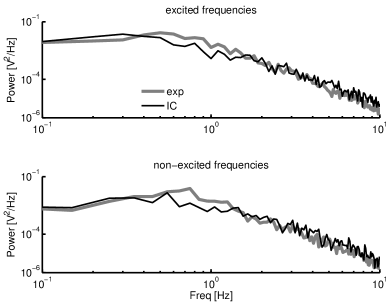
(a) Control signal (instruction “cc”)

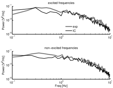
(b) Control signal (instruction “ol”)

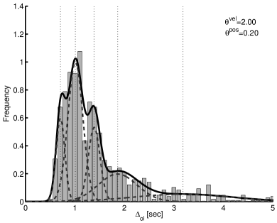
(c) $\Delta_{ol}$ (instruction “cc”)

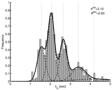
(d) $\Delta_{ol}$ (instruction “ol”)

Figure 32: Variability resulting from event-driven IC. The top graphs show the resulting fit to experimental data at excited and non-excited frequencies. The bottom graphs show the distribution of intermittent intervals, together with the optimal threshold values.

The corresponding thresholds (for “cc”: $\theta^{v}=2.0,\,\theta^{p}=0.2$, for “mi”: $\theta^{v}=2.1,\,\theta^{p}=0.8$) reflect the control priorities for each instruction: for “cc” position control should be prioritised, resulting in a small value for the position threshold, while the velocity is relatively unimportant. For “mi” the control intervention should be minimal, which is associated with large thresholds on both, velocity and position.

Figures 32(c) and 32(d) show the distributions of the open loop intervals for each condition, together with an approximation by a series of weighted Gaussian distributions (McLachlan and Peel, 2000). For position control (“cc”), open loop intervals are clustered around a modal interval of approximately 1s, with all $\Delta_{ol}>0.5$s. For the minimal intervention condition (“mi”), the open loop intervals are clustered around a modal interval of approximately 2s, and all $\Delta_{ol}>1$s. This corresponds to the expected behaviour of the human operator where more frequent updates of the intermittent control trajectory are associated with the more demanding position control instruction, while the instruction to minimise intervention results in longer intermittent intervals. Thus the identified thresholds not only result in IC models which approximate the response at excited and non-excited frequency, but also reflect the underlying control aims.

8.4 Conclusion

The hypothesis that variability is the result of a continuous control process with added noise (PC with added noise), requires that the remnant is explained by a non-parametric input noise component. In comparison, IC introduces variability as a result of a small number of threshold parameters which are clearly related to underlying control aims.

9 Identification of intermittent control: the underlying continuous system

This section, together with Section 10, addresses the question of how intermittency can be identified when observing closed loop control. In this Section it is discussed how intermittent control can masquerade as continuous control, and how the underlying continuous system can be identified. Section 10 addresses the question how intermittency can be detected in experimental data.

System identification provides one approach to hypothesis testing and has been used by Johansson et al. (1988) and Peterka (2002) to test the non-predictive hypothesis and by Gawthrop et al. (2009) to test the non-predictive and predictive hypotheses. Given time domain data from an sustained control task which is excited by an external disturbance signal, a two stage approach to controller estimation can be used in order to perform the parameter estimation in the frequency domain: firstly, the frequency response function is estimated from measured data, and secondly, a parametric model is fitted to the frequency response using non-linear optimisation (Pintelon and Schoukens, 2001; Pintelon et al., 2008). This approach has two advantages: firstly, computationally expensive analysis of long time-domain data sets can be reduced by estimation in the frequency domain, and secondly, advantageous properties of a periodic input signal (as advocated by Pintelon et al. (2008)) can be exploited.

In this section, first the derivation of the underlying frequency responses for a predictive continuous time controller and for the intermittent, clock-driven controller (i.e. $\Delta_{ol}=\text{const}$) is discussed. The method is limited to clock-driven IC since frequency analysis tools are readily available only for this case (Gawthrop, 2009). The two stage identification procedure is then outlined, followed by example results from a visual-manual control task.

The material in this section is partially based on Gollee et al. (2012).

9.1 Closed-loop frequency response

As a prerequisite for system identification in the frequency domain, this section looks at the frequency response of closed-loop system corresponding to the underlying predictive continuous design method as well as that of the intermittent controller with a fixed intermittent interval (Gawthrop, 2009).

9.1.1 Predictive continuous control

The system equations (2.1) can be rewritten in transfer function form as

$$y_{o}(s) =G(s)u(s)$$

$$\text{with }G(s) =C\left[sI-A\right]^{-1}B$$ (9.1)

where $I$ is the $n\times n$ unit matrix and $s$ denotes the complex Laplace operator.

Transforming equations (2.2) and (2.5) into the Laplace domain, assuming that disturbances $v_{u}$, $v_{u}$ and $w$ are zero:

$${\mathbf{x}_{o}}(s) =\left(sI-A_{o}\right)^{-1}(Bu(s)+Ly_{o}(s))\;\;$$ (Observer) (9.2)

$${x_{p}}(s) =e^{A\Delta}\hat{x}(s)+\left(sI-A\right)^{-1}\left(I-e^{-(sI-A)\Delta}\right)Bu(s)\;\;$$ (Predictor) (9.3)

$$u(s) =-ke^{-s\Delta}{{x}_{p}}(s)$$ (Controller) (9.4)

where $I$ is the $n\times n$ unit matrix.

Equations (9.2)–(9.4) can be rewritten as:

$$u(s) =-e^{-s\Delta}\left[H_{y}(s)y(s)+(H_{1}(s)+H_{2}(s))u(s)\right]$$ (9.5)

$$\text{where }H_{y}(s) =ke^{A\Delta}\left(sI-A_{o}\right)^{-1}L$$ (9.6)

$$H_{1}(s) =ke^{A\Delta}\left(sI-A_{o}\right)^{-1}B$$ (9.7)

$$\text{and }H_{2}(s) =k\left(sI-A\right)^{-1}\left(I-e^{-(sI-A)\Delta}\right)Be^{s\Delta}$$ (9.8)

It follows that the controller transfer function $H(s)$ is given by:

$$H(s)=\frac{H_{y}(s)}{1+H_{1}(s)+H_{2}(s)}$$ (9.9)

where

$$\frac{u(s)}{y_{o}(s)}=-e^{-s\Delta}H(s)$$ (9.10)

With equations (9.1) and (9.10), the system loop-gain $L(s)$ and closed-loop transfer function $T$ are given by:

$$L(s) =e^{-s\Delta}G(s)H(s)$$ (9.11)

$$T(s) =\frac{u(s)}{d(s)}=\frac{L(s)}{1+L(s)}$$ (9.12)

Equation (9.12) gives a parametrised expression relating $u(s)$ and $d(s)$.

9.1.2 Intermittent Control

The sampling operation in Figure 2 makes it harder to derive a (continuous-time) frequency response and so the details are omitted here. For the case were the intermittent interval is assumed to be constant, the basic result derived by Gawthrop (2009) apply and can be encapsulated as the following theorem:

Theorem

The continuous-time system (2.1) controlled by an intermittent controller with generalised hold gives a closed-loop system where the Fourier transform $\mathbf{U}$ of the control signal $u(t)$ is given in terms of the Fourier transform $\mathbf{X^{d}}(j\omega)$ by

$$\mathbf{U}=F(j\omega,\theta)\left[\mathbf{X^{d}}(j\omega)\right]^{s}\\$$ (9.13)

where

$$F(j\omega,\theta) =\mathbf{H}(j\omega)\mathbf{S_{z}}(e^{j\omega})$$ (9.14)

$$\mathbf{H}(j\omega) =\frac{1}{\Delta_{ol}}\mathbf{k}\left[j\omega I-A_{c}\right]^{-1}\left[I-e^{-(j\omega I-A_{c})\Delta_{ol}}\right]$$ (9.15)

$$\mathbf{S_{z}}(e^{j\omega}) =[I+\mathbf{G_{z}}(e^{j\omega})]^{-1}$$ (9.16)

$$\mathbf{G_{z}}(e^{j\omega}) =\left[e^{j\omega}I-A_{x}\right]^{-1}B_{x}$$ (9.17)

$$\mathbf{X^{d}}(j\omega) =\mathbf{G}(j\omega)\mathbf{d}(j\omega)$$ (9.18)

$$\mathbf{G}(j\omega) =[j\omega I-A]^{-1}B$$ (9.19)

The sampling operator is defined as

$$\left[\mathbf{X^{d}}(j\omega)\right]^{s}=\sum_{k=-\infty}^{\infty}\mathbf{\mathbf{X}^{d}}(j\omega-kj\omega_{ol})$$ (9.20)

where the intermittent sampling-frequency is given by $\omega_{ol}=2\pi/\Delta_{ol}$.

As discussed in Gawthrop (2009), the presence of the sampling operator $\left[\mathbf{X^{d}}(j\omega)\right]^{s}$ means that the interpretation of $F(j\omega,\theta)$ is not quite the same as that of the closed loop transfer function $T(s)$ of (9.12), as the sample process generates an infinite number of frequencies which can lead to aliasing. As shown in Gawthrop (2009), the (bandwidth limited) observer acts as an anti-aliasing filter, which limits the effect of $\left[\mathbf{X^{d}}(j\omega)\right]^{s}$ to higher frequencies and makes $F(j\omega,\theta)$ a valid approximation of $\mathbf{U}$. $F(j\omega,\theta)$ will therefore be treated as equivalent to $T(j\omega)$ in the rest of this Section.

9.2 System identification

The aim of the identification procedure is to derive an estimate for the closed-loop transfer function of the system. Our approach follows the two stage procedure of Pintelon and Schoukens (2001) and Pintelon et al. (2008). In the first step, the frequency response transfer function is estimated based on measured input–output data, resulting in a non-parametric estimate. In the second step, a parametric model of the system is fitted to the estimated frequency response using an optimisation procedure.

9.2.1 System setup

To illustrate the approach, we consider the visual-manual control task described in Section 8.1, where the subject is asked to sustain control of an unstable 2nd order load using a joystick, with the instruction to keep the load as close to the centre as possible (“cc”).

9.2.2 Non-parametric estimation

In the first step, a non-parametric estimate of the closed loop frequency response function (FRF) is derived, based on observed input–output data. The system was excited by a multi-sine disturbance signal (equation (8.2)). The output $u(t)$ of a linear system which is excited by $d(t)$ then only contains information at the same discrete frequencies $\omega_{k}$ as the input signal. If the system is non-linear or noise is added, the output will contain a remnant component at non-excited frequencies as discussed in Section 8. several periods was used.

The time domain signals $d(t)$ and $u(t)$ over one period $T_{0}$ of the excitation signal were transformed into the frequency domain. If the input signal has been applied over $N_{p}$ periods, then the frequency-domain data for the $l$th period can be denoted as $d^{[l]}(j\omega_{k})$ and $u^{[l]}(j\omega_{k})$, respectively, and the FRF can be estimated as

$$\hat{T}^{[l]}(j\omega_{k})=\frac{u^{[l]}(j\omega_{k})}{d^{[l]}(j\omega_{k})},\qquad k=1,2,\dots,N_{f}$$ (9.21)

where $N_{f}$ denotes the number of frequency components in the excitation signal. An estimate of the FRF over all $N_{p}$ periods is obtained by averaging,

$$\hat{T}(j\omega_{k})=\frac{1}{N_{p}}\sum_{l=1}^{N_{p}}\hat{T}^{[l]}(j\omega_{k}),\qquad k=1,2,\dots,N_{f}$$ (9.22)

This approach ensures that only the periodic (deterministic) features related to the disturbance signal are used in the identification, and that the identification is robust with respect to remnant components.

9.2.3 Parametric optimisation

In the second stage of the identification procedure, a parametric description, $\tilde{T}(j\omega_{k},\theta)$, is fitted to the estimated FRF of equation (9.22). The parametric FRF approximates the closed loop transfer function (equation (9.12)) which depends in the case of predictive control, on the loop transfer function $L(j\omega_{k},\theta)$, equation (9.11), parametrised by the vector $\theta$, while for the intermittent controller this is approximated by $F(j\omega,\theta)$, equation (9.13),

$$\tilde{T}(j\omega_{k},\theta)=\begin{cases}\frac{L(j\omega_{k},\theta)}{1+L(j\omega_{k},\theta)}&\text{for PC}\\ F(j\omega_{k},\theta)&\text{for IC}\end{cases}$$ (9.23)

We use an indirect approach to parametrise the controller, where the controller and observer gains are derived from optimised design parameters using the standard LQR approach of equation (2.6). This allows the specification of boundaries for the design parameters which guarantee a nominally stable closed loop system. As described in Section 2.3, the feedback gain vector $k$ can then be obtained by choosing the elements of the matrices $Q_{c}$ and $R_{c}$ in (2.6), and nominal stability can be guaranteed if these matrices are positive definite. As the system model is second order, we choose to parametrise the design using two positive scalars, $q_{v}$ and $q_{p}$,

$$R_{c}=1\qquad Q_{c}=\left[\begin{array}[]{c c}q_{v}&0\\ 0&q_{p}\end{array}\right],\text{ with }q_{v},\,q_{p}>0$$ (9.24)

related to relative weightings of the velocity ($q_{v}$) and position ($q_{p}$) states.

The observer gain vector $L$ is obtained by applying the same approach to the dual system $[A^{T},C^{T},B^{T}]$. It was found that the results are relatively insensitive to observer properties which was therefore parametrised by a single positive variable, $q_{o}$,

$$R_{o}=1\qquad Q_{o}=q_{o}\,BB^{T}\text{ with }q_{o}>0$$ (9.25)

where $R_{o}$ and $Q_{o}$ correspond to $R_{c}$ and $Q_{c}$ in equation (2.6) for the dual system.

The controller can then be fully specified by the positive parameter vector $\theta=[q_{v},q_{p},q_{o},\Delta]$ (augmented by $\Delta_{ol}$ for intermittent control).

The optimisation criterion $J$ is defined as the mean squared difference between the estimated FRF and its parametric fit

$$J(\theta)=\frac{1}{N_{f}}\sum_{k=1}^{N_{f}}\left[\hat{T}(j\omega_{k})-\tilde{T}(j\omega_{k},\theta)\right]^{2}$$ (9.26)

This criterion favours lower frequency data since $|T(j\omega)|$ tends to be larger in this range.

The parameter vector is separated into two parts, time delay parameters,

$$\theta_{\Delta}=\begin{cases}[\Delta]&\text{for PC}\\ [\Delta,\Delta_{ol}]&\text{for IC}\end{cases}$$ (9.27)

and controller design parameters

$$\theta_{c}=[q_{v},q_{p},q_{o}]$$ (9.28)

such that $\theta=\left[\theta_{\Delta},\theta_{c}\right]$. The time delay parameters are varied over a predefined range, with the restriction that $\Delta_{ol}>\Delta$ for IC. For each given set of time delay parameters, a corresponding set of optimal controller design parameters $\theta^{*}_{c}$ is found which solves the constrained optimisation problem

$$\theta_{c}^{*}=\arg\min_{\theta_{c}}J([\theta_{\Delta},\theta_{c}]),\qquad\theta_{c}>0$$ (9.29)

which was solved using the SQP algorithm (Nocedal and Wright, 2006), (MATLAB Optimization Toolbox, Mathworks, USA).

The optimal cost function for each set of time-delay parameters, $J^{*}(\theta_{\Delta})$, was calculated, and the overall optimum, $J^{*}$ determined. For analysis, the time-delay parameters corresponding to the optimal cost are determined, with $\Delta$ and $\Delta_{ol}$ combined for the IC to give the effective time-delay,

$$\Delta_{e}=\Delta+0.5\Delta_{ol}$$ (9.30)

9.3 Illustrative example

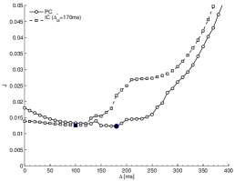
(a) Cost function.

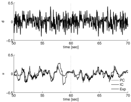
(b) Time domain signals.

(c) Nyquist plot of the FRF.

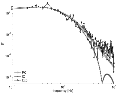
(d) Bode magnitude plot of the FRF

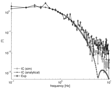
(e) Bode magnitude plot of FRF for IC.

Figure 33: Illustrative experimental results. (a) shows the optimisation cost (equation (9.26)) as a function of the time delay for predictive continuous control (PC) and intermittent control (IC), together with the value of the intermittent interval corresponding to the smallest cost ($\Delta^{*}_{ol}$). (b)-(d) show comparisons between predictive continuous control (PC), intermittent control (IC) and the experimental data (Exp). Plots for PC and IC in (c) and (d) are derived analytically (equation (9.23)). (e) compares the analytical FRF for the IC with the FRF derived from time-domain simulation data.

Results from identifying the experimental data from one subject are used to illustrate the approach.

An extract of the time domain data are shown in Figure 33(b). The top plot shows the multi-sine disturbance input over two 10sec periods, and the bottom plot depicts the corresponding measured control signal response (thin dark line). From this response, the experimental FRF was estimated in stage 1 of the identification (dark solid lines in Figures 33(c)–33(e)).

Stage 2 of the procedure aimed to find the controller design parameters which resulted in the best fit to the experimental FRF. The corresponding cost functions for the predictive continuous and for the intermittent controller are shown in Figure 33(a), with the minima indicated by solid markers. The estimated FRF (equation (9.22)) and their parametric fits (equation (9.23)) are shown in Figure 33(c). It is clear that both the PC and IC are able to fit the experimental FRF equally well. The resulting controller parameters (summarised in table 1) are very similar for both control architectures. This is confirmed by time-domain simulations using the estimated controllers (Figure 33(b)) where the PC and IC responses are difficult to distinguish.

	PC	IC
$q_{p}$	0.99	1.07
$q_{v}$	0.00	0.00
$q_{o}$	258.83	226.30
$\Delta$	180ms	95ms
$\Delta_{ol}$	–	170ms
$\Delta_{e}$	–	180ms

Table 1: Estimated controller design parameters

Although the Nyquist plot of Figure 33(c) suggests that the PC and IC responses are virtually identical, further analysis shows that this is only the case at lower frequencies (at which most of the signal power lies). The Bode plot of the frequency response (Figure 33(d)) shows that the PC and IC are indistinguishable only for frequencies up to around 2-3Hz. This is also the frequency range up to which the PC and IC provide a good approximation to the experimental FRF.

The controller frequency responses shown in Figures 33(c) and 33(d) are based on the analytically derived expressions. For the IC, the sampling operator means that the theoretical response is only a valid approximation at lower frequencies, with aliasing evident at higher frequencies. A comparison of the analytical response with the response derived from simulated time-domain data (Figure 33(e)) shows that the simulated frequency response of the IC at higher frequency is in fact closer to the experimental data than the analytical response.

9.4 Conclusions

The results illustrate that continuous predictive and intermittent controllers can be equally valid descriptions of a sustained control task. Both approaches allow fitting the estimated non-parametric frequency responses with comparable quality. This implies that experimental data can be equally well explained using the PC and the IC hypotheses. This result is particularly interesting as it means that experimental results showing good fit for continuous predictive control models, dating back to at least those of Kleinman et al. (1970), do not rule out an intermittent explanation. A theoretical explanation for this result is given in (Gawthrop et al., 2011, Section 4.3) where the masquerading property of intermittent control is discussed: As shown there (and illustrated in the results here), the frequency response of an intermittent controller and that of the corresponding predictive controller are indistinguishable at lower frequency and only diverge at higher frequencies where aliasing occurs. Thus, the responses of the predictive and the intermittent controllers are difficult to distinguish, and therefore both explanations appear to be equally valid.

10 Identification of intermittent control: Detecting intermittency

As discussed in Section 3 and by Gawthrop et al. (2011), the key feature distinguishing intermittent control from continuous control is the open-loop interval $\Delta_{ol}$ of Equations (3.1) and (3.5). As noted in Sections 3.1 and 4.2, the open-loop interval provides an explanation of the Psychological Refractory Period (PRP) of Telford (1931) as discussed by Vince (1948) to explain the human response to double stimuli. Thus “intermittency” and “refractoriness” are intimately related. Within this interval, the control trajectory is open loop but is continuously time varying according to the basis of the generalised hold. The length of the intermittent interval gives a trade-off between continuous control (zero intermittent interval) and intermittency. Continuous control maximises the frequency bandwidth and stability margins at the cost of reduced flexibility whereas intermittent control provides time in the loop for optimisation and selection (van de Kamp et al., 2013a; Loram et al., 2014) at the cost of reduced frequency bandwidth and reduced stability margins. The rationale for intermittent control is that it confers online flexibility and adaptability. This rationale has caused many investigators to consider whether intermittent control is an appropriate paradigm for understanding biological motor control (Craik, 1947a, b; Vince, 1948; Bekey, 1962; Navas and Stark, 1968; Neilson et al., 1988; Miall et al., 1993a; Hanneton et al., 1997; Neilson and Neilson, 2005; Loram and Lakie, 2002). However, even though intermittent control was first proposed in the physiological literature in 1947, there has not been an adequate methodology to discriminate intermittent from continuous control and to identify key parameters such as the open loop interval $\Delta_{ol}$. Within the biological literature, four historic planks of evidence (discontinuities, frequency constancy, coherence limit and psychological refractory period) have provided evidence of intermittency in human motor control (Loram et al., 2014).

1. The existence of discontinuities within the control signal has been interpreted as sub-movements or serially planned control sequences (Navas and Stark, 1968; Poulton, 1974; Miall et al., 1993a, 1986; Hanneton et al., 1997; Loram and Lakie, 2002),

2. Constancy in the modal rate of discontinuities, typically around 2-3 per second, has been interpreted as evidence for a central process with a well defined timescale (Navas and Stark, 1968; Poulton, 1974; Lakie and Loram, 2006; Loram et al., 2006).

3. The fact that coherence between unpredicted disturbance or set-point and control signal is limited to a low maximum frequency, typically of 1-2 Hz, below the mechanical bandwidth of the feedback loop has been interpreted as evidence of sampling (Navas and Stark, 1968; Loram et al., 2009, 2011).

4. The psychological refractory period has provided direct evidence of open loop intervals but only for discrete movements and serial reaction time (e.g. push button) tasks and has not been demonstrated for sustained sensori-motor control (Vince, 1948; Pashler and Johnston, 1998; Hardwick et al., 2013).

Since these features can be reproduced by a continuous controller with tuned parameters and filtered additive noise (Levison et al., 1969; Loram et al., 2012), this evidence is circumstantial. Furthermore, there is no theoretical requirement for regular sampling nor for discontinuities in control trajectory. Indeed, as historically observed by Craik (1947a, b), humans tend to smoothly join control trajectories following practice. Therefore the key methodological problem is to demonstrate that on-going control is sequentially open loop even when the control trajectory is smooth and when frequency analysis shows no evidence of regular sampling.

10.1 Outline of method

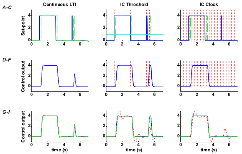
Figure 34: Reconstruction of the set-point. Example responses to set-point step-sequence A–C. Solid: two paired steps (long inter-step interval, short inter-step interval) are applied to the set-point of each of three models: continuous linear time invariant, threshold triggered intermittent control (unit threshold), and clock triggered (zero threshold) intermittent control (cols 1–3 respectively). Dashed: Set-point adjusted: time of each step follows preceding trigger by one model time delay (${\Delta}$). D–F. Solid: Control output (ue). Red vertical dashed: event trigger times. G–I. Solid: Control output (ue). Dash-dotted: ARMA (LTI) fit to set-point (solid in A–C). Dashed: ARMA (LTI) fit to adjusted set-point (dashed in A–C). [(Loram et al., 2012) Copyright ©2012 the authors. Used with permission.]

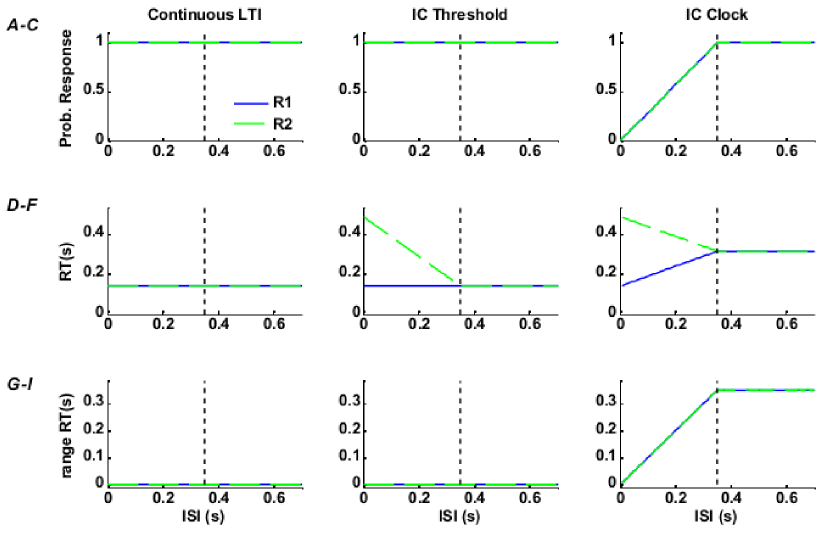
Figure 35: Reconstruction of the set-point. Predicted delays for varying inter-step interval For three models continuous linear time invariant, threshold triggered intermittent control and clock triggered intermittent control (cols 1–3 respectively) the following is shown as a function of inter-step interval (ISI):- A–C. The predicted probability of response D–F. The mean response delay G–I. The range of response delays Response 1 and 2 (R1, R2) are solid and dashed respectively. For these calculations the open loop interval ($\Delta_{ol}$) is 0.35s (vertical dashed line) and feedback time-delay (td) is 0.14s. [(Loram et al., 2012) Copyright ©2012 the authors. Used with permission.]

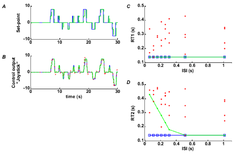
Figure 36: Reconstruction of the set-point. Representative Stage 1 Analysis A. Solid: Set-point sequence containing 8 inter-step-interval pairs with random direction (first 30s). Dashed: adjusted set-point from step 1 analysis. After a double unidirectional step, set-point returns to zero before next pair. B. Solid: Control output (ue). Dash-dotted: ARMA (LTI) fit to set-point. Dashed: ARMA (LTI) fit to adjusted set-point. C, D. Response times (RT1, RT2) respectively from each of three models v Inter-step-interval (ISI). Joined square: Continuous LTI. Joined dot: Threshold intermittent control. Isolated dot: Clock intermittent control. The system is zero order. The open loop interval ($\Delta_{ol}$) is 0.35s and feedback time-delay (${\Delta}$) is 0.14s. [(Loram et al., 2012) Copyright ©2012 the authors. Used with permission.]

Using the intermittent-equivalent setpoint of Sections 3.7 and 4.2, we summarise a method to distinguish intermittent from continuous control (Loram et al., 2012). The identification experiment uses a specially designed paired-step set-point sequence. The corresponding data analysis uses a conventional ARMA model to relate the theoretically derived equivalent set-point (of Section 3.7) to the control signal. The method sequentially and iteratively adjusts the timing of the steps of this equivalent set-point to optimise the linear time invariant fit. The method has been verified using realistic simulation data and was found to robustly distinguish not only between continuous and intermittent control but also between event-driven intermittent and clock-driven intermittent control (Loram et al., 2012). This identification method is applicable for machine and biological applications. For application to humans the set-point sequence should be unpredictable in the timing and direction of steps. This method proceeds in three stages. Stages 1 and 2 are independent of model assumptions and quantify refractoriness, the key feature discriminating intermittent from continuous control.

10.1.1 Stage 1: Reconstruction of the set-point

With reference to Figure 34, this stage takes the known set-point and control output signals and reconstructs the set-point step times to form that sequence with a linear-time invariant response which best matches the control output. This is implemented as an optimisation process in which the fit of a general linear time series model (zero-delay ARMA) is maximised by adjusting the trial set of step times. The practical algorithmic steps are stated by Loram et al. (2012). The output from stage 1 is an estimate of the time delay for each step stimulus.

10.1.2 Stage 2: Statistical analysis of delays:

Delays are classified according to step (1 or 2, named reaction-time 1 (RT1) and reaction-time 2 (RT2) respectively) and inter-step-interval (ISI). A significant difference in delay, RT2 v. RT1, is not explained by a linear-time-invariant model. The reaction time properties, or refractoriness, is quantified by:

1. the size of ISI for which RT2 $>$ RT1. This indicates the temporal separation required to eliminate interference between successive steps and

2. the difference in delay (RT2 $-$ RT1).

10.1.3 Stage 3: Model based interpretation:

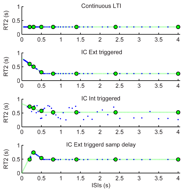
Figure 37: Model-based interpretation (stage 3). Parameter variants from the generalised IC model of figure 2 showing several possible relationships between RT2 and inter-step interval (ISI) indicative of serial ballistic (intermittent) and continuous control behaviour. The simulated system is zero order. The open-loop interval ($\Delta_{ol}$) is 0.55s and feedback time delay (${\Delta}$) is 0.25s. For four models: A) continuous LTI ($\Delta_{ol}=0$), B) externally-triggered intermittent control with a prediction error threshold, C) internally-triggered intermittent control (with zero prediction error threshold, triggered to saturation), and D) externally-trigger intermittent control supplemented with a sampling delay of 0.25s which is associated with the ISI at the maximum delay for RT2. The joined green circles represent the theoretical delays as a function of ISI which are confirmed by the model simulations (blue dots). [(van de Kamp et al., 2013a) Copyright ©2012 the authors. Used with permission.]

For controllers following the generalised continuous (Figure 1) and intermittent (Figure 2) structures, the probability of a response occurring, the mean delay and the range of delays can be predicted for each inter-step-interval (Figure 35 and Appendix C of Loram et al. (2012)). For a continuous controller (Figure 1) all delays equal the model delay (${\Delta}$). Intermittent control is distinguished from continuous control by increased delays for RT2 v. RT1 for inter-step-intervals less than the open-loop interval ($\Delta_{ol}$). Clock (zero threshold) triggered intermittent control is distinguished from threshold triggered intermittent control by the range of delays for RT1 and RT2 and by the increased mean delay for inter-step intervals greater than the open-loop interval ($\Delta_{ol}$) (Figure 3). If the results of Stage 1–2 analysis conform to these patterns (Figure 35), the open-loop interval ($\Delta_{ol}$) can be estimated. Simulation also shows that the sampling delay ($\Delta_{s}$) can be identified from the ISI at which the delay RT2 is maximal (Fig 37) (van de Kamp et al., 2013a, b). Following verification by simulation (Loram et al., 2012), the method has been applied to human visually guided pursuit tracking and to whole body pursuit tracking. In both cases control has been shown to be intermittent rather than continuous.

10.2 Refractoriness in sustained manual control

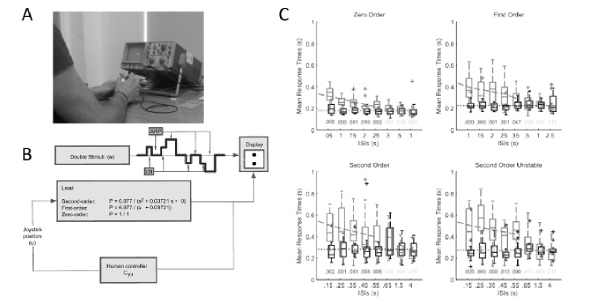
Figure 38: Refractoriness in sustained manual control. A. Task setup. An oscilloscope showed real-time system output position as a small focused dot with negligible delay. Participants provided input to the system using a sensitive, uniaxial, contactless joystick. The system ran in Simulink Real-Time Windows Target within the MATLAB environment (Math-Works). B. Control system and experimental set up. Participants were provided with a tracking target in addition to system output. The tracking signal was constructed from four possible patterns of step sequence (uni- and reversed directional step to the left or to the right). First and second stimuli are separated by an unpredictable inter step interval (ISI), patterns are separated by an unpredictable approximate recovery period (ARP). The participant was only aware of an unpredictable sequence of steps. C. Group results: The four panels: Zero Order, First Order, Second Order, Second Order Unstable show the inter participant mean first (RT1, black) and second (RT2, gray) response times against Inter step intervals (ISIs), p-values of the ANOVA’s post hoc test are displayed above each ISI level (dark if significant, light if not). [ (van de Kamp et al., 2013b). Copyright ©2013 the authors. Used with permission.]

Using a uni-axial, sensitive, contactless joystick, participants were asked to control four external systems (zero, first, second order stable, second order unstable) using visual feedback to track as fast and accurately as possible the target which changes position discretely and unpredictably in time and direction (Figures 38A&B). For the zero, first and second order systems, joystick position determines system output position, velocity and acceleration respectively. The unstable second order system had a time-constant equivalent to a standing human. Since the zero order system has no dynamics requiring ongoing control, step changes in target produce discrete responses i.e. sharp responses clearly separated from periods of no response. The first and second order systems require sustained ongoing control of the system output position: thus the step stimuli test responsiveness during ongoing control. The thirteen participants showed evidence of substantial open loop interval (refractoriness) which increased with system order (0.2 to 0.5 s, 38 C). For first and second order systems, participants showed evidence of a sampling delay (0.2-0.25 s, 38 C). This evidence of refractoriness discriminates against continuous control.

10.3 Refractoriness in whole body control

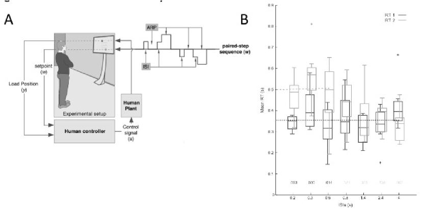
Figure 39: Refractoriness in whole body control A. The participant receives visual feed-back of the Anterior-Posterior head position through a dot presented on an LCD screen mounted on a trolley. Without moving their feet, participants were asked to track the position of a second dot displayed on the screen. The four possible step sequence combinations (uni- and reversed-directional step up or down) of the pursuit target are illustrated by the solid line. First and second stimuli are separated by an inter-step interval (ISI). The participant experiences an unpredictable sequence of steps. B. Group results. Figure shows the inter-participant mean RT1 (black) and RT2 (gray) against ISI combined across the eight participants. The P-values of the ANOVA’s post-hoc test are display above each ISI level (black if ¡0.05, gray if not). The dotted line shows the mean RT1, the dashed line shows the regression linear fit between (interfered) RT2 and ISIs. [(van de Kamp et al., 2013a). Copyright ©2013 the authors. Used with permission.]

Control of the hand muscles may be more refined, specialised and more intentional than control of the muscles serving the legs and trunk (van de Kamp et al., 2013a). Using online visual feedback ($<$ 100 ms delay) of a marker on the head, participants were asked to track as fast and accurately as possible a target which changes position discretely and unpredictably in time and direction (Figure 39A). This required head movements of 2cm along the anterior-posterior axis and while participants were instructed not to move their feet, no other constraints or strategies were requested. The eight participants showed evidence of substantial open loop interval (refractoriness) ( 0.5 s) and a sampling delay ( 0.3 s) (39 B). This result extends the evidence of intermittent control from sustained manual control to integrated intentional control of the whole body.

11 Adaptive intermittent control

The purpose of feedback control is to reduce uncertainty (Horowitz, 1963; Jacobs, 1974). Feedback control using fixed controllers can be very successful in this role as long as sufficient bandwidth is available and the system does not contain time delays or other non-minimum phase elements (Horowitz, 1963; Goodwin et al., 2001; Skogestad and Postlethwaite, 1996). However, when the system and actuators do contain such elements, an adaptive controller can be used to reduce uncertainly and thus, in time, improve controller performance. By its nature, intermittent control is a low-bandwidth controller and so adaptation is particularly appropriate in this context. Conversely, intermittent control frees computing resources that can be used for this purpose.

As discussed in the textbooks by Goodwin and Sin (1984) and by Åström and Wittenmark (1989) adaptive control of engineering systems is well established. Perhaps the simplest approach is to combine real-time recursive parameter estimation with a simple controller design method to give a so called “self-tuning” strategy (Åström and Wittenmark, 1973; Clarke and Gawthrop, 1975, 1979, 1981; Åström and Wittenmark, 1989). However, such an approach ignores two things: the controller is based on initially incorrect parameter estimates and the quality of the parameter estimation is dependent on the controller properties. This can be formalised using the concepts of caution whereby the adaptive controller takes account of parameter uncertainty and probing whereby the controller explicitly excites the system to improve parameter estimation (Jacobs and Patchell, 1972; Bar-Shalom, 1981). Adaptive controllers which explicitly and jointly optimise controller performance and parameter estimation have been called dual controllers (Feldbaum, 1960; Bar-Shalom and Tse, 1974). Except in simple cases, for example that of Astrom and Helmersson (1986), the solution to the dual control problem is impractically complex.

Since Wiener (1965) developed the idea of cybernetics, there has been a strong interest in applying both biologically-inspired and engineering-inspired ideas to adaptive control in both humans and machines; ideas arising from the biological and engineering inspired fields have been combined in various ways.

One such thread is reinforcement learning (Sutton and Barto, 1998) which continues to be developed both theoretically and through applications (Khan et al., 2012). It can be argued that that “reinforcement learning is direct adaptive optimal control” (Sutton et al., 1992). Artificial neural networks have been applied to engineering control systems: see the survey of Hunt et al. (1992) and numerous textbooks (Miller et al., 1990; Żbikowski and Hunt, 1996; Kalkkuhl et al., 1997). Recent work is described by Vrabie and Lewis (2009). Again, there are links between Artificial Neural Network (ANN) methods such as back-propagation and engineering parameter estimation (Gawthrop and Sbarbaro, 1990).

Field robotics makes use of the concept of Simultaneous Location and Mapping (SLAM) (Durrant-Whyte and Bailey, 2006; Bailey and Durrant-Whyte, 2006). Roughly speaking, location corresponds to state estimation and mapping to parameter estimation and therefore concepts and techniques from SLAM are appropriate to adaptive (intermittent) control. In particular, the Extended Kalman Filter (EKF) and the Unscented Kalman Filter (UKF) (Julier et al., 2000; Schiff, 2012) provide the basis for SLAM and hence adaptive control.

In this section the simplest continuous-time self-tuning approach (Gawthrop, 1982, 1987, 1990) is used. As indicated in the Examples of Sections 12 and 13, this simple approach has interesting behaviours; neverthless, it would be interesting to investigate more sophisticated approaches based on, for example, the EKF and UKF.

11.1 System Model

Parameter estimation is much simplified if the system can be transformed into linear-in-the-parameters (LIP) form; the resultant model can be viewed as a non-minimal state-space (NMSS) representation of the system. The NMSS approach is given in discrete-time form by Young et al. (1987) and continuous-time form by Taylor et al. (1998). Although a purely state-space approach to the NMSS representation is possible (Gawthrop et al., 2007), a polynomial approach is simpler and is presented here.

The linear-time invariant system considered in this Chapter are given in Laplace transform terms by:

$${\bar{y}(s)}=\frac{b(s)}{a(s)}\left({\bar{u}(s)}+\frac{b_{\xi}(s)}{a_{\xi}(s)}{\bar{\xi}_{u}(s)}\right)+\frac{{\mathbf{d}^{\prime}}(s)}{a(s)a_{\xi}(s)}$$ (11.1)

where ${\bar{y}(s)}$, ${\bar{u}(s)}$, and ${\bar{\xi}_{u}(s)}$ are the Laplace transformed system output, control input and input disturbance. $\frac{b(s)}{a(s)}$ is the transfer function relating ${\bar{y}(s)}$ and ${\bar{u}(s)}$ and $\frac{b_{\xi}(s)}{a_{\xi}(s)}$ provides a transfer function model of the input disturbance. It is assumed that both transfer functions are strictly proper. The overall system initial conditions are represented by the polynomial ${\mathbf{d}^{\prime}}(s)$. The polynomials $a(s)$, $b(s)$ and ${\mathbf{d}^{\prime}}(s)$ are of the form:

$$a(s) =a_{0}s^{n}+a_{1}s^{n-1}+\dots+a_{n}$$ (11.2)

$$b(s) =b_{1}s^{n-1}+\dots+b_{n}$$ (11.3)

$${\mathbf{d}^{\prime}}(s) ={\mathbf{d}^{\prime}}_{1}s^{n-1}+\dots+{\mathbf{d}^{\prime}}_{n}$$ (11.4)

$$a_{\xi}(s) =\alpha_{0}s^{n_{\xi}}+\alpha_{1}s^{n_{\xi}-1}+\dots+\alpha_{n_{\xi}}$$ (11.5)

$$b_{\xi}(s) =\beta_{0}s^{n_{\xi}}+\beta_{1}s^{n_{\xi}-1}+\dots+\beta_{n_{\xi}}$$ (11.6)

Finally, defining the Hurwitz polynomial $c(s)$ as:

$$c(s) =c_{0}s^{N}+c_{1}s^{N-1}+\dots+c_{N}$$ (11.7)

$$\text{where }N =n+n_{\xi}+1$$ (11.8)

Equation (11.1) may be rewritten as:

$$\frac{a(s)a_{\xi}(s)}{c(s)}{\bar{y}(s)}=\frac{b(s)a_{\xi}(s)}{c(s)}{\bar{u}(s)}+\frac{b(s)b_{\xi}(s)}{c(s)}{\bar{\xi}_{u}(s)}+\frac{{\mathbf{d}^{\prime}}(s)}{c(s)}$$ (11.9)

For the purposes of this Chapter, the polynomials $a_{\xi}(s)$, $b_{\xi}(s)$ are defined as:

$$a_{\xi}(s) =s$$ (11.10)

$$b_{\xi}(s) =1$$ (11.11)

With this choice, Equation (11.9) simplifies to

$$\frac{sa(s)}{c(s)}{\bar{y}(s)}=\frac{sb(s)}{c(s)}{\bar{u}(s)}+\frac{b(s)}{c(s)}{\bar{\xi}_{u}(s)}+\frac{d(s)}{c(s)}$$ (11.12)

In the special case that the input disturbance is a jump to a constant value $d_{\xi}$ at time $t=0^{+}$, then this can be modelled using Equations (11.10) and (11.11) and

$$\xi(t) =d_{\xi}\delta(t)$$ (11.13)

$$\text{and }{\bar{\xi}_{u}(s)} =d_{\xi}$$ (11.14)

where $\delta(t-t_{k}$ is the Dirac delta function.

Equation (11.9) then becomes:

$$\frac{sa(s)}{c(s)}{\bar{y}(s)} =\frac{sb(s)}{c(s)}{\bar{u}(s)}+\frac{d(s)}{c(s)}$$ (11.15)

$$\text{where }d(s) ={\mathbf{d}^{\prime}}(s)+d_{\xi}b(s)$$ (11.16)

Equation (11.12) can be rewritten in non-minimal state-space form as:

$$\frac{d}{dt}\phi_{y}(t) =A_{s}\phi_{y}(t)-B_{s}y(t)$$ (11.17)

$$\frac{d}{dt}\phi_{u}(t) =A_{s}\phi_{u}(t)+B_{s}u(t)$$ (11.18)

$$\frac{d}{dt}\phi_{ic}(t) =A_{s}\phi_{ic}(t),\;\phi_{ic}(0)=\phi_{ic0}$$ (11.19)

$$\text{where }A_{s} =\begin{bmatrix}\begin{matrix}-c_{1}&-c_{2}&\dots&-c_{N-1}&-c_{N}\\ 1&0&\dots&0&0\\ 0&1&\dots&0&0\\ \dots&\dots&\dots&\dots&\dots\\ 0&0&\dots&0&0\\ 0&0&\dots&1&0\\ \end{matrix}\end{bmatrix}$$ (11.20)

$$\text{and }B_{s} =\begin{bmatrix}1\\ 0\\ \dots\\ 0\end{bmatrix}$$ (11.21)

It follows that:

$$\epsilon(t) =\theta^{T}\phi(t)$$ (11.22)

$$\text{where }\theta =\begin{bmatrix}\mathbf{a}\\ \mathbf{b}\\ \mathbf{d}\end{bmatrix}\text{ and }\phi(t)=\begin{bmatrix}\phi_{y}\\ \phi_{u}\\ \phi_{ic}\end{bmatrix}$$ (11.23)

$$\text{and }\mathbf{a} =\begin{bmatrix}a_{0}&a_{1}&\dots&a_{n}&\mathbf{0}\end{bmatrix}^{T}$$ (11.24)

$$\mathbf{b} =\begin{bmatrix}0&b_{1}&\dots&b_{n}&\mathbf{0}\end{bmatrix}^{T}$$ (11.25)

$$\mathbf{d} =\begin{bmatrix}0&d_{1}&\dots&d_{n}&\dots&d_{n_{c}}\end{bmatrix}^{T}$$ (11.26)

11.2 Continuous-time Parameter Estimation

As discussed by Young (1981), Gawthrop (1982, 1987), Unbehauen and Rao (1987, 1990) and Garnier and Wang (2008), least-squares parameter estimation can performed in the continuous-time domain (as opposed to the more usual discrete-time domain as described, for example, by Ljung (1999)). A brief outline of the method used in the following examples is given in this section.

$${e_{h}}(t) =\hat{\theta}_{u}^{T}\phi(t)$$ (11.27)

$$J(\hat{\theta}_{u}) =\frac{1}{2}\int_{0}^{t}e^{\lambda(t-t^{\prime})}{e_{h}}(t^{\prime})^{2}dt^{\prime}$$

$$=\hat{\theta}_{u}^{T}\mathbf{S}(t)\hat{\theta}_{u}$$

$$=\hat{\theta}_{u}^{T}\mathbf{S}_{uu}(t)\hat{\theta}_{u}+\hat{\theta}_{u}^{T}\mathbf{S}_{uk}(t)\theta_{k}+\theta_{k}^{T}\mathbf{S}_{kk}(t)\theta_{k}$$ (11.28)

$$\text{where }\mathbf{S}(t) =\int_{0}^{t}e^{\lambda(t-t^{\prime})}\phi(t^{\prime})\phi^{T}(t^{\prime})dt^{\prime}$$ (11.29)

and the symmetrical matrix $\mathbf{S}(t)$ has been partitioned as:

$$\mathbf{S}(t)=\begin{bmatrix}\mathbf{S}_{uu}(t)&\mathbf{S}_{uk}(t)\\ \mathbf{S}^{T}_{uk}(t)&\mathbf{S}_{kk}(t)\end{bmatrix}$$ (11.31)

Differentiating the cost function $J$ with respect to the vector of unknown parameters $\hat{\theta}_{u}$ gives:

$$\frac{dJ}{d\hat{\theta}_{u}}=\mathbf{S}_{uu}(t)\hat{\theta}_{u}+\mathbf{S}_{uk}(t)\theta_{k}$$ (11.32)

Setting the derivative to zero gives the optimal solution:

$$\hat{\theta}_{u}(t)=-\mathbf{S}_{uu}^{-1}(t)\mathbf{S}_{uk}(t)\theta_{k}$$ (11.33)

Differentiating $\mathbf{S}$ (11.29) with respect to time gives

$$\frac{d\mathbf{S}}{dt}+\lambda\mathbf{S}(t)=\phi(t)\phi^{T}(t)$$ (11.34)

11.3 Intermittent Parameter Estimation

The incremental information matrix ${\tilde{\mathbf{S}}}_{i}$ from the $i$th intermittent interval is defined as

$${\tilde{\mathbf{S}}}_{i}=\int_{t_{i-1}}^{t_{i}}\phi(t^{\prime})\phi^{T}(t^{\prime})dt^{\prime}$$ (11.35)

Equation (11.35) may be implemented using the differential equation (11.34) with zero initial condition at time $t_{i-1}$. The intermittent information matrix $\mathbf{S}_{i}$ at the $i$th intermittent interval is defined as:

$$\mathbf{S}_{i}=\lambda_{ic}\mathbf{S}_{i-1}+{\tilde{\mathbf{S}}}_{i}$$ (11.36)

Partitioning $\mathbf{S}_{i}$ as Equation (11.31) gives the parameter estimate of Equation (11.33).

If there is a disturbance characterised by Equations (11.10), (11.11) and (11.14), the parameters corresponding to $d(s)$ jump when the disturbance jumps. As such a jump will give rise to an event, a new set of $d$ parameters should be estimated; this is achieved by adding a diagonal matrix to the elements of $\mathbf{S}_{i}$ corresponding to $d(s)$.

12 Examples: adaptive human balance

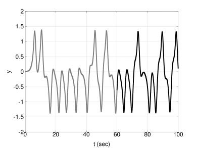
(a) Output $y$. No adaption $\Delta b_{0}=0$

(b) Phase-plane. No adaption $\Delta b_{0}=0$

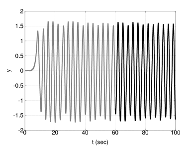
(c) Output $y$. No adaption $\Delta b_{0}=0.1$

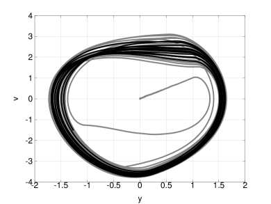
(d) Phase-plane. No adaption $\Delta b_{0}=0.1$

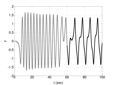
(e) Output $y$. Adaption $\Delta b_{0}=0.1$

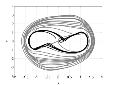
(f) Phase-plane. Adaption $\Delta b_{0}=0.1$

Figure 40: Adaptive Balance control. (a)&(b) Correct parameters, no adaptation. (c)&(d) Incorrect parameters, no adaptation. (e)&(f) Incorrect parameters, with adaptation – the initial behaviour corresponds to (c)&(d) and the final behaviour corresponds to (a)&(b). For clarity, lines are coloured grey for $t<60$ and black for $t\geq 60$.

Figure 41: Adaptive Balance control: estimated Parameter. The parameter estimate errors ($\hat{a}-a$ and $\hat{b}-b$) become smaller as time increases.

As discussed by Gawthrop et al. (2014), it can be argued that the human balance control system generates ballistic control trajectories that attempt to place the unstable system at equilibrium; this leads to homoclinic orbits (Hirsch et al., 2012). However, such behaviour is dependent on a good internal model. This section looks at the same ballistic balance control system as that of Gawthrop et al. (2014) but in the context of parameter adaptation.

The controlled system is given by the transfer function:

$$G(s)=\frac{b}{s^{2}+a}$$ (12.1)

The actual system parameters are:

$$a =-1$$ (12.2)

$$b =1.1$$ (12.3)

The parameters $a$ and $b$ are estimated using the intermittent parameter estimation method of Section 11.3 with initial values:

$$\hat{a} =-1$$ (12.4)

$$\hat{b} =1$$ (12.5)

Figures 40(a) and 40(b) show the non-adaptive controller with correct parameters of Equations (12.2) and (12.3); the behaviour approximates that of the ideal ballistic controller.

Figures 40(c) and 40(d) show the non-adaptive controller with the incorrect parameters of Equations (12.4) and (12.5); the behaviour is now a limit cycle.

Figures 40(e) and 40(f) shows the adaptive controller with the initial incorrect parameters of Equations (12.4) and (12.5). Initially, the behaviour corresponds to that of Figures 40(a) and 40(b); but after about 50sec the behaviour corresponds to that of Figures 40(c) and 40(d). The corresponding parameter estimate errors ($\hat{a}-a$ and $\hat{b}-b$) are given in Figure 41.

13 Examples: adaptive human reaching

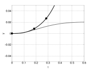
(a) $y$, 1st iter.

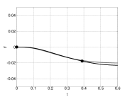
(b) $y$, 50th iter.

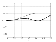
(c) $y$, 51st iter.

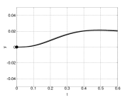
(d) $y$, 100th iter.

(e) $u$, 1st iter.

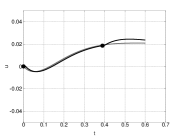
(f) $u$, 50th iter.

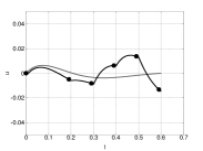
(g) $u$, 51st iter.

(h) $u$, 100th iter.

Figure 42: Reaching in a force-field: transverse position. The additional transverse force field is applied throughout, but the initial parameters correspond to zero force field. The sample instants are denoted by the $\bullet$ symbol. The behaviour improves, and the intermittent interval increases, from iteration 1 to iteration 50.

(a) 1st iter.

(b) 25th iter.

(c) 50th iter.

(d) 51st iter.

(e) 100th iter.

Figure 43: Reaching in a force-field. The data from Figure 42 are re-plotted against longitudinal position.

(a) $\hat{a}$

Figure 44: Reaching in a force-field: parameters. The transverse force field parameter is $a=-100$ for $0\leq\text{iteration}\leq 50$ and $a=0$ for $\text{iteration}>50$. The initial estimate is $\hat{a}=0$.

Repetitive reaching and pointing has been examined by a number of authors including Shadmehr and Mussa-Ivaldi (1994) (see also Shadmehr and Mussa-Ivaldi (2012)), Burdet et al. (2006) and Tee et al. (2010). An iterative learning control explanation of these results is given by Zhou et al. (2012).

As discussed by Bristow et al. (2006), “iterative learning control (ILC) is based on the notion that the performance of a system that executes the same task multiple times can be improved by learning from previous executions (trials, iterations, passes).”. A number of survey papers are available, including those of Bristow et al. (2006), Ahn et al. (2007) and Wang et al. (2009), as well as a book Xu and Tan (2003). ILC is closely related to repetitive control (Cuiyan et al., 2004) and to multi-pass control (Edwards, 1974; Owens, 1977).

This example shows how the intermittent parameter estimation method of Section 11.3 can be used in the context of iterative learning.

The system similar to that described in Section IV, case 3 of the paper by Zhou et al. (2012) was used. The lateral motion of the arm in the force field was described the transfer function of Equation (12.1) with

$$a =\begin{cases}-100&i\leq 50\\ 0&i>50\end{cases}$$ (13.1)

$$b =100$$ (13.2)

The lateral target position was randomly set to $\pm 0.01$m.

The parameters $a$ and $b$ are estimated using the intermittent parameter estimation method of Section 11.3 with initial values:

$$\hat{a} =0$$ (13.3)

$$\hat{b} =200$$ (13.4)

Figure 42 shows the system output (transverse position) $y$ and control input $u$ for five of the iterations; the sample instants are denoted by the $\bullet$ symbol and the ideal trajectory by the grey line. The initial behaviour (Figures 42(a) and 42(e)) is unstable and sampling occurs at the minimum interval of 100ms the behaviour at the 50th iteration (Figures 42(b) and 42(f))just before the parameter change is close to ideal even though the trajectory is open loop for nearly 400ms. The behaviour at the 51st iteration (Figures 42(c) and 42(g)) just after the parameter change is again poor (although stable) but has become ideal and open loop by iteration 100 (Figures 42(d) and 42(h)). The data is replotted in Figure 43 to show the transverse position $y$ plotted against longitudinal position.

Figure 44 shows the evolution of the estimated parameters with iteration number.

14 Conclusion

• This chapter has given an overview of the current state-of-the-art of the event-driven Intermittent Control discussed, in the context of physiological systems, by Gawthrop et al. (2011). In particular, Intermittent Control has been shown to provide a basis for the human control systems associated with balance and motion control.

• Intermittent control arose in the context of applying control to systems and constraints which change through time (Ronco et al., 1999). The intermittent control solution allows slow optimisation to occur concurrently with a fast control action. Adaptation is intrinsic to intermittent control and yet the formal relationship between adaptive and intermittent control remains to be established. Some results of experiments with human subjects reported by Loram et al. (2011), together with the simulations of Sections 12 and 13, support the intuition that the intermittent interval somehow simplifies the complexities of dual control . A future challenge is to provide a theoretical basis formally linking intermittent and adaptive control. This basis would extend applicability of time varying control and would enhance investigation of biological controllers which are adaptive by nature.

• It is an interesting question as to where the event-driven intermittent control algorithm lies in the human nervous system. IC provides time within the feedback loop to use the current state to select new motor responses (control structure, law, goal, constraints). This facility provides competitive advantage in performance, adaptation and survival and is thus likely to operate through neural structures which are evolutionarily old as well as new (Brembs, 2011). Refractoriness in humans is associated with a-modal response selection rather than sensory processing or motor execution (Pashler and Johnston, 1998). This function suggests plausible locations within premotor regions and within the slow striatal-prefrontal gating loops (Jiang and Kanwisher, 2003; Dux et al., 2006; Houk et al., 2007; Seidler, 2010; Battaglia-Mayer et al., 2014; Loram et al., 2014).

• It seems plausible that Intermittent Control has applications within a broader biomedical context. Some possible areas are:

  Rehabilitation

  practice, following neuromuscular disease such as stroke and spinal cord injury, often uses passive closed loop learning in which movement is externally imposed by therapists or assistive technology (e.g. robotic assisted rehabilitation (Huang and Krakauer, 2009)). Loram et al. (2011) have shown that adaptation to parameter changes during human visual-manual control can be facilitated by using an explicitly intermittent control strategy. For successful learning, active user input should excite the system, allowing learning from the observed intermittent open-loop behaviour (Loram et al., 2011).

  Cellular control systems

  in general and gene regulatory networks in particular seem to have a intermittent nature (Albeck et al., 2008; Balazsi et al., 2011; Liu and Jiang, 2012). It would be interesting to examine whether the intermittent control approaches of this paper are relevant in the context of cellular control systems.

• The particular Intermittent control algorithm discussed within this Chapter has roots and applications in control engineering (Ronco et al., 1999; Gawthrop and Wang, 2006, 2009a; Gawthrop et al., 2012) and it is hoped that this chapter will lead to further cross-fertilisation of physiological and engineering research. Some possible areas are:

  Decentralised control

  (Sandell et al., 1978; Bakule and Papik, 2012) is a pragmatic approach to the control of large-scale systems where, for reasons of cost, convenience and reliability it is not possible to control the entire system by a single centralised controller. Fundamental control-theoretic principles arising from decentralised control have been available for some time (Clements, 1979; Anderson and Clements, 1981; Gong and Aldeen, 1992). More recently, following the implementation of decentralised control using networked control systems (Moyne and Tilbury, 2007), attention has focused on the interaction of communication and control theory (Baillieul and Antsaklis, 2007; Nair et al., 2007) and fundamental results have appeared (Nair and Evans, 2003; Nair et al., 2004; Hespanha et al., 2007). It would be interesting to apply the physiologically inspired approaches of this Chapter to decentralised control as well as to reconsider Intermittent Control in the context of decentralised control systems.

  Networked control systems

  lead to the “sampling period jitter problem” (Sala, 2007; Moyne and Tilbury, 2007) where uncertainties in transmission time lead to unpredictable non-uniform sampling and stability issues (Cloosterman et al., 2009). A number of authors have suggested that performance may be improved by replacing the standard zero-order hold by a generalised hold (Feuer and Goodwin, 1996; Sala, 2005, 2007) or using a dynamical model of the system to interpolate between samples (Zhivoglyadov and Middleton, 2003; Montestruque and Antsaklis, 2003). This can be shown to improve stability (Montestruque and Antsaklis, 2003; Hespanha et al., 2007). As shown by Gawthrop and Wang (2011), the intermittent controller has a similar feature; it therefore follows that the physiologically inspired form of intermittent controller described in this chapter has application to networked control systems.

  Robotics.

  It seems likely that understanding the control mechanisms behind human balance and motion control (Loram et al., 2009; van de Kamp et al., 2013a, b) and stick balancing (Gawthrop et al., 2013b) will have applications in robotics. In particular, as discussed by van de Kamp et al. (2013a), robots, like humans contain redundant possibilities within a multi-segmental structure. Thus the multivariable constrained intermittent control methods illustrated in Section 7, and the adaptive versions illustrated in Section 11 may well be applicable to the control of autonomous robots.

References

- Åström and Wittenmark (1973) K. J. Åström and B. Wittenmark. On self-tuning regulators. Automatica, 9:185–199, 1973. doi:10.1016/0005-1098(73)90073-3.
- Åström and Wittenmark (1989) K. J. Åström and B. Wittenmark. Adaptive Control. Addison-Wesley, 1989.
- Ahn et al. (2007) Hyo-Sung Ahn, YangQuan Chen, and K.L. Moore. Iterative learning control: Brief survey and categorization. Systems, Man, and Cybernetics, Part C: Applications and Reviews, IEEE Transactions on, 37(6):1099 –1121, Nov. 2007. ISSN 1094-6977. doi:10.1109/TSMCC.2007.905759.
- Albeck et al. (2008) John G Albeck, John M Burke, Sabrina L Spencer, Douglas A Lauffenburger, and Peter K Sorger. Modeling a snap-action, variable-delay switch controlling extrinsic cell death. PLoS Biol, 6(12):e299, 12 2008. doi:10.1371/journal.pbio.0060299.
- Alexandrov et al. (2005) AV. Alexandrov, AA. Frolov, FB. Horak, P. Carlson-Kuhta, and S. Park. Feedback equilibrium control during human standing. Biological Cybernetics, 93:309–322, November 2005. doi:10.1007/s00422-005-0004-1.
- Anderson and Clements (1981) Brian D.O. Anderson and David J. Clements. Algebraic characterization of fixed modes in decentralized control. Automatica, 17(5):703 – 712, 1981. ISSN 0005-1098. doi:10.1016/0005-1098(81)90017-0.
- Asai et al. (2009) Yoshiyuki Asai, Yuichi Tasaka, Kunihiko Nomura, Taishin Nomura, Maura Casadio, and Pietro Morasso. A model of postural control in quiet standing: Robust compensation of delay-induced instability using intermittent activation of feedback control. PLoS ONE, 4(7):e6169, 07 2009. doi:10.1371/journal.pone.0006169.
- Astrom (1977) K. J. Astrom. Frequency domain properties of Otto Smith regulators. International Journal of Control, 26:307–314, 1977. ISSN 0020-7179. doi:10.1080/00207177708922311.
- Astrom and Bernhardsson (2002) K. J. Astrom and B. M. Bernhardsson. Comparison of Riemann and Lebesgue sampling for first order stochastic systems. In Decision and Control, 2002, Proceedings of the 41st IEEE Conference on, volume 2, pages 2011–2016 vol.2, January 2002.
- Astrom and Bernhardsson (2003) Karl Astrom and Bo Bernhardsson. Systems with Lebesgue sampling. In Anders Rantzer and Christopher Byrnes, editors, Directions in Mathematical Systems Theory and Optimization, pages 1–13. Springer, 2003. ISBN 978-3-540-00065-5. doi:10.1007/3-540-36106-5.
- Astrom (2008) Karl J. Astrom. Event based control. In Alessandro Astolfi and Lorenzo Marconi, editors, Analysis and Design of Nonlinear Control Systems, pages 127–147. Springer, Heidelberg, 2008. ISBN 978-3-540-74357-6. doi:10.1007/978-3-540-74358-3.
- Astrom and Helmersson (1986) K.J. Astrom and A. Helmersson. Dual control of an integrator with unknown gain. Computers and Mathematics with Applications, 12(6, Part A):653 – 662, 1986. ISSN 0898-1221. doi:10.1016/0898-1221(86)90052-0.
- Bailey and Durrant-Whyte (2006) T. Bailey and H. Durrant-Whyte. Simultaneous localization and mapping (SLAM): part II. Robotics Automation Magazine, IEEE, 13(3):108 –117, sept. 2006. ISSN 1070-9932. doi:10.1109/MRA.2006.1678144.
- Baillieul and Antsaklis (2007) J. Baillieul and P.J. Antsaklis. Control and communication challenges in networked real-time systems. Proceedings of the IEEE, 95(1):9 –28, jan. 2007. ISSN 0018-9219. doi:10.1109/JPROC.2006.887290.
- Bakule and Papik (2012) Lubomir Bakule and Martin Papik. Decentralized control and communication. Annual Reviews in Control, 36(1):1 – 10, 2012. ISSN 1367-5788. doi:10.1016/j.arcontrol.2012.03.001.
- Balazsi et al. (2011) Gabor Balazsi, Alexander van Oudenaarden, and James J. Collins. Cellular decision making and biological noise: From microbes to mammals. Cell, 144(6):910 – 925, 2011. ISSN 0092-8674. doi:10.1016/j.cell.2011.01.030.
- Bar-Shalom (1981) Y. Bar-Shalom. Stochastic dynamic programming: Caution and probing. Automatic Control, IEEE Transactions on, 26(5):1184 – 1195, oct 1981. ISSN 0018-9286. doi:10.1109/TAC.1981.1102793.
- Bar-Shalom and Tse (1974) Y. Bar-Shalom and E. Tse. Dual effect, certainty equivalence, and separation in stochastic control. Automatic Control, IEEE Transactions on, 19(5):494 – 500, oct 1974. ISSN 0018-9286. doi:10.1109/TAC.1974.1100635.
- Baron et al. (1970) S. Baron, D. L. Kleinman, and W. H. Levison. An optimal control model of human response part ii: Prediction of human performance in a complex task. Automatica, 6:371–383, May 1970. doi:10.1016/0005-1098(70)90052-X.
- Barrett and Glencross (1988) Nicholas C. Barrett and Denis J. Glencross. The double step analysis of rapid manual aiming movements. The Quarterly Journal of Experimental Psychology Section A, 40(2):299–322, 1988. doi:10.1080/02724988843000131.
- Battaglia-Mayer et al. (2014) Alexandra Battaglia-Mayer, Tania Buiatti, Roberto Caminiti, Stefano Ferraina, Francesco Lacquaniti, and Tim Shallice. Correction and suppression of reaching movements in the cerebral cortex: Physiological and neuropsychological aspects. Neuroscience & Biobehavioral Reviews, 42:232–251, May 2014. doi:10.1016/j.neubiorev.2014.03.002.
- Bekey (1962) George A. Bekey. The human operator as a sampled-data system. Human Factors in Electronics, IRE Transactions on, HFE-3(2):43–51, Sept. 1962. doi:10.1109/THFE2.1962.4503341.
- Bhushan and Shadmehr (1999) Nikhil Bhushan and Reza Shadmehr. Computational nature of human adaptive control during learning of reaching movements in force fields. Biol. Cybern., 81(1):39–60, July 1999. doi:10.1007/s004220050543.
- Bottaro et al. (2005) Alessandra Bottaro, Maura Casadio, Pietro G. Morasso, and Vittorio Sanguineti. Body sway during quiet standing: Is it the residual chattering of an intermittent stabilization process? Human Movement Science, 24(4):588 – 615, 2005. ISSN 0167-9457. doi:10.1016/j.humov.2005.07.006.
- Bottaro et al. (2008) Alessandra Bottaro, Youko Yasutake, Taishin Nomura, Maura Casadio, and Pietro Morasso. Bounded stability of the quiet standing posture: An intermittent control model. Human Movement Science, 27(3):473 – 495, 2008. ISSN 0167-9457. doi:10.1016/j.humov.2007.11.005.
- Boyd and Vandenberghe (2004) S.P. Boyd and L. Vandenberghe. Convex optimization. Cambridge Univ Press, 2004. ISBN 0 521 83378 7.
- Brembs (2011) Bjorn Brembs. Towards a scientific concept of free will as a biological trait: spontaneous actions and decision-making in invertebrates. Proceedings of the Royal Society B: Biological Sciences, 278(1707):930–939, 2011. doi:10.1098/rspb.2010.2325.
- Bristow et al. (2006) D.A. Bristow, M. Tharayil, and A.G. Alleyne. A survey of iterative learning control. Control Systems, IEEE, 26(3):96 – 114, june 2006. ISSN 1066-033X. doi:10.1109/MCS.2006.1636313.
- Burdet et al. (2006) E. Burdet, K. Tee, I. Mareels, T. Milner, C. Chew, D. Franklin, R. Osu, and M. Kawato. Stability and motor adaptation in human arm movements. Biological Cybernetics, 94:20–32, 2006. ISSN 0340-1200. doi:10.1007/s00422-005-0025-9.
- Chen and Gawthrop (2006) Wen-Hua Chen and Peter J. Gawthrop. Constrained predictive pole-placement control with linear models. Automatica, 42(4):613–618, April 2006. doi:10.1016/j.automatica.2005.09.020.
- Clarke and Gawthrop (1975) D. W. Clarke and P. J. Gawthrop. Self-tuning controller. IEE Proceedings Part D: Control Theory and Applications, 122(9):929–934, 1975. doi:10.1049/piee.1975.0252.
- Clarke and Gawthrop (1979) D. W. Clarke and P. J. Gawthrop. Self-tuning Control. IEE Proceedings Part D: Control Theory and Applications, 126(6):633–640, 1979. doi:10.1049/piee.1979.0145.
- Clarke and Gawthrop (1981) D. W. Clarke and P. J. Gawthrop. Implementation and application of microprocessor-based self-tuners. Automatica, 17(1):233–244, 1981. doi:10.1016/0005-1098(81)90098-4.
- Clements (1979) David J. Clements. A representation result for two-input two-output decentralized control systems. The Journal of the Australian Mathematical Society. Series B. Applied Mathematics, 21(1):113–127, 1979. doi:10.1017/S0334270000001971.
- Cloosterman et al. (2009) Marieke B. G. Cloosterman, Nathan van de Wouw, W. P. M. H. Heemels, and Hendrik Nijmeijer. Stability of networked control systems with uncertain time-varying delays. IEEE Transactions on Automatic Control,, 54(7):1575–1580, July 2009. doi:10.1109/TAC.2009.2015543.
- Craik (1947a) Kenneth J Craik. Theory of human operators in control systems: Part 1, the operator as an engineering system. British Journal of Psychology, 38:56–61, 1947a. doi:10.1111/j.2044-8295.1947.tb01141.x.
- Craik (1947b) Kenneth J Craik. Theory of human operators in control systems: Part 2, man as an element in a control system. British Journal of Psychology, 38:142–148, 1947b. doi:10.1111/j.2044-8295.1948.tb01149.x.
- Cuiyan et al. (2004) Li Cuiyan, Zhang Dongchun, and Zhuang Xianyi. A survey of repetitive control. In Intelligent Robots and Systems, 2004. (IROS 2004). Proceedings. 2004 IEEE/RSJ International Conference on, volume 2, pages 1160–1166 vol.2, Sept.-2 Oct. 2004. doi:10.1109/IROS.2004.1389553.
- Durrant-Whyte and Bailey (2006) H. Durrant-Whyte and T. Bailey. Simultaneous localization and mapping (SLAM): part I. Robotics Automation Magazine, IEEE, 13(2):99 –110, june 2006. ISSN 1070-9932. doi:10.1109/MRA.2006.1638022.
- Dux et al. (2006) Paul E. Dux, Jason Ivanoff, Christopher L. Asplund, and Ren Marois. Isolation of a central bottleneck of information processing with time-resolved fMRI. Neuron, 52(6):1109 – 1120, 2006. ISSN 0896-6273. doi:10.1016/j.neuron.2006.11.009.
- Edwards (1974) J.B. Edwards. Stability problems in the control of multipass processes. Electrical Engineers, Proceedings of the Institution of, 121(11):1425 –1432, november 1974. ISSN 0020-3270. doi:10.1049/piee.1974.0299.
- Feldbaum (1960) A.A. Feldbaum. Optimal control theory. Academic Press, New York, 1960.
- Feuer and Goodwin (1996) A. Feuer and G.C. Goodwin. Sampling in Digital Signal Processing and Control. Birkhauser, Berlin, 1996.
- Fletcher (1987) R. Fletcher. Practical Methods of Optimization. 2nd Edition. Wiley, Chichester, 1987.
- Foo and Weyer (2011) M. Foo and E. Weyer. On reproducing existing controllers as model predictive controllers. In Australian Control Conference (AUCC), 2011, pages 303 –308, nov. 2011.
- Franklin and Powell (1980) G. F. Franklin and J. D. Powell. Digital Control of Dynamic Systems. Addison-Wesley, Reading, Massachusetts, 1980.
- Franklin et al. (1994) G. F. Franklin, J. D. Powell, and A. Emami-Naeini. Feedback Control of Dynamic Systems (3rd edition). Addison-Wesley, 1994.
- Fuller (1968) A. T. Fuller. Optimal nonlinear control systems with pure delay. Int. J. Control, 8:145–168, 1968. doi:10.1080/00207176808905662.
- Garnier and Wang (2008) Hugues Garnier and Liuping Wang, editors. Identification of continuous-time models from sampled data. Advances in Industrial Control. Springer, London, 2008.
- Gawthrop (1976) P. J. Gawthrop. Studies in identification and control. D.Phil. thesis, Oxford University, 1976. URL http://ora.ox.ac.uk/objects/uuid:90ade91d-df67-42ef-a422-0d3500331701.
- Gawthrop (1982) P. J. Gawthrop. A continuous-time approach to discrete-time self-tuning control. Optimal Control: Applications and Methods, 3(4):399–414, 1982.
- Gawthrop (1987) P. J. Gawthrop. Continuous-time Self-tuning Control. Vol 1: Design. Research Studies Press, Engineering control series., Lechworth, England., 1987.
- Gawthrop (1990) P. J. Gawthrop. Continuous-time Self-tuning Control. Vol 2: Implementation. Research Studies Press, Engineering control series., Taunton, England., 1990.
- Gawthrop and Sbarbaro (1990) P. J. Gawthrop and D. G. Sbarbaro. Stochastic approximation and multilayer perceptrons: The gain back-propagation algorithm. Complex System Journal, 4:51–74, 1990.
- Gawthrop and Wang (2011) Peter Gawthrop and Liuping Wang. The system-matched hold and the intermittent control separation principle. International Journal of Control, 84(12):1965–1974, 2011. doi:10.1080/00207179.2011.630759.
- Gawthrop et al. (2009) Peter Gawthrop, Ian Loram, and Martin Lakie. Predictive feedback in human simulated pendulum balancing. Biological Cybernetics, 101(2):131–146, 2009. doi:10.1007/s00422-009-0325-6. Published online July 09, 2009.
- Gawthrop et al. (2011) Peter Gawthrop, Ian Loram, Martin Lakie, and Henrik Gollee. Intermittent control: A computational theory of human control. Biological Cybernetics, 104(1-2):31–51, 2011. doi:10.1007/s00422-010-0416-4. Published online: 17th February 2011.
- Gawthrop et al. (2013a) Peter Gawthrop, Henrik Gollee, Adamantia Mamma, Ian Loram, and Martin Lakie. Intermittency explains variability in human motor control. In NeuroEng 2013: Australian Workshop on Computational Neuroscience, Melbourne, Australia, 2013a. (Abstract only).
- Gawthrop et al. (2013b) Peter Gawthrop, Kwee-Yum Lee, Mark Halaki, and Nicholas O’Dwyer. Human stick balancing: an intermittent control explanation. Biological Cybernetics, 107(6):637–652, 2013b. ISSN 0340-1200. doi:10.1007/s00422-013-0564-4. Published online: 13th August 2013.
- Gawthrop et al. (2013c) Peter Gawthrop, David Wagg, Simon Neild, and Liuping Wang. Power-constrained intermittent control. International Journal of Control, 86(3):396–409, 2013c. doi:10.1080/00207179.2012.733888. Published online 30 Oct 2012.
- Gawthrop et al. (2014) Peter Gawthrop, Ian Loram, Henrik Gollee, and Martin Lakie. Intermittent control models of human standing: similarities and differences. Biological Cybernetics, 108(2):159–168, 2014. ISSN 0340-1200. doi:10.1007/s00422-014-0587-5. Published online 6th February 2014.
- Gawthrop (2009) Peter J Gawthrop. Frequency domain analysis of intermittent control. Proceedings of the Institution of Mechanical Engineers Pt. I: Journal of Systems and Control Engineering, 223(5):591–603, 2009. doi:10.1243/09596518JSCE759.
- Gawthrop and Gollee (2012) Peter J Gawthrop and Henrik Gollee. Intermittent tapping control. Proceedings of the Institution of Mechanical Engineers, Part I: Journal of Systems and Control Engineering, 226(9):1262–1273, 2012. doi:10.1177/0959651812450114. Published online on July 26, 2012.
- Gawthrop and Ronco (2002) Peter J Gawthrop and Eric Ronco. Predictive pole-placement control with linear models. Automatica, 38(3):421–432, March 2002. doi:10.1016/S0005-1098(01)00231-X.
- Gawthrop and Wang (2006) Peter J. Gawthrop and Liuping Wang. Intermittent predictive control of an inverted pendulum. Control Engineering Practice, 14(11):1347–1356, November 2006. doi:10.1016/j.conengprac.2005.09.002.
- Gawthrop and Wang (2007) Peter J Gawthrop and Liuping Wang. Intermittent model predictive control. Proceedings of the Institution of Mechanical Engineers Pt. I: Journal of Systems and Control Engineering, 221(7):1007–1018, 2007. doi:10.1243/09596518JSCE417.
- Gawthrop and Wang (2009a) Peter J. Gawthrop and Liuping Wang. Constrained intermittent model predictive control. International Journal of Control, 82:1138–1147, 2009a. ISSN 0020-7179. doi:10.1080/00207170802474702. Published online 27 January 2009.
- Gawthrop and Wang (2009b) Peter J Gawthrop and Liuping Wang. Event-driven intermittent control. International Journal of Control, 82(12):2235 – 2248, December 2009b. doi:10.1080/00207170902978115. Published online 09 July 2009.
- Gawthrop and Wang (2010) Peter J. Gawthrop and Liuping Wang. Intermittent redesign of continuous controllers. International Journal of Control, 83:1581–1594, 2010. ISSN 0020-7179. doi:10.1080/00207179.2010.483691.
- Gawthrop et al. (2007) Peter J. Gawthrop, Liuping Wang, and Peter C. Young. Continuous-time non-minimal state-space design. Int. J. Control, 80(10):690 – 1697, 2007. doi:10.1080/00207170701546006. Published on-line: 26 July 2007.
- Gawthrop et al. (2012) Peter J. Gawthrop, Simon A. Neild, and David J. Wagg. Semi-active damping using a hybrid control approach. Journal of Intelligent Material Systems and Structures, 2012. doi:10.1177/1045389X12436734. Published online February 21, 2012.
- Gawthrop et al. (2008) P.J. Gawthrop, M.D. Lakie, and I.D. Loram. Predictive feedback control and Fitts’ law. Biological Cybernetics, 98(3):229–238, March 2008. doi:10.1007/s00422-007-0206-9. Published online: 5 January 2008.
- Gollee et al. (2012) H. Gollee, A. Mamma, I. D. Loram, and P. J. Gawthrop. Frequency-domain identification of the human controller. Biological Cybernetics, 106:359–372, 2012. ISSN 0340-1200. doi:10.1007/s00422-012-0503-9. Published online: 14 July 2012.
- Gong and Aldeen (1992) Z. Gong and M. Aldeen. On the characterization of fixed modes in decentralized control. Automatic Control, IEEE Transactions on, 37(7):1046 –1050, jul 1992. ISSN 0018-9286. doi:10.1109/9.148369.
- Goodwin and Sin (1984) G. C. Goodwin and K. S. Sin. Adaptive Filtering Prediction and Control. Prentice-Hall, Englewood Cliffs, New Jersey, USA, 1984.
- Goodwin et al. (2001) G.C. Goodwin, S.F. Graebe, and M.E. Salgado. Control System Design. Prentice Hall, New Jersey, 2001.
- Günther et al. (2009) Michael Günther, Sten Grimmer, Tobias Siebert, and Reinhard Blickhan. All leg joints contribute to quiet human stance: A mechanical analysis. Journal of Biomechanics, 42(16):2739 – 2746, 2009. ISSN 0021-9290. doi:10.1016/j.jbiomech.2009.08.014.
- Günther et al. (2011) Michael Günther, Otto Müller, and Reinhard Blickhan. Watching quiet human stance to shake off its straitjacket. Archive of Applied Mechanics, 81(3):283–302, 2011. ISSN 0939-1533. doi:10.1007/s00419-010-0414-y.
- Günther et al. (2012) Michael Günther, Otto Müller, and Reinhard Blickhan. What does head movement tell about the minimum number of mechanical degrees of freedom in quiet human stance? Archive of Applied Mechanics, 82(3):333–344, 2012. ISSN 0939-1533. doi:10.1007/s00419-011-0559-3.
- Hanneton et al. (1997) S. Hanneton, A. Berthoz, J. Droulez, and J.J.E. Slotine. Does the brain use sliding variables for the control of movements? Biological Cybernetics, 77(6):381 – 393, December 1997. doi:10.1007/s004220050398.
- Hardwick et al. (2013) Robert M. Hardwick, Claudia Rottschy, R. Chris Miall, and Simon B. Eickhoff. A quantitative meta-analysis and review of motor learning in the human brain. NeuroImage, 67(0):283 – 297, 2013. ISSN 1053-8119. doi:10.1016/j.neuroimage.2012.11.020.
- Heemels et al. (2008) W. Heemels, JH Sandee, and P.P.J.V.D. Bosch. Analysis of event-driven controllers for linear systems. International Journal of Control, 81(4):571–590, 2008. doi:10.1080/00207170701506919.
- Hespanha et al. (2007) J.P. Hespanha, P. Naghshtabrizi, and Yonggang Xu. A survey of recent results in networked control systems. Proceedings of the IEEE, 95(1):138 –162, jan. 2007. ISSN 0018-9219. doi:10.1109/JPROC.2006.887288.
- Hirsch et al. (2012) M.W. Hirsch, S. Smale, and R.L. Devaney. Differential Equations, Dynamical Systems, and an Introduction to Chaos. Academic Press, third edition, 2012. ISBN 978-0-12-382010-5.
- Hogan (1984) N. Hogan. Adaptive control of mechanical impedance by coactivation of antagonist muscles. Automatic Control, IEEE Transactions on, 29(8):681–690, 1984. ISSN 0018-9286. doi:10.1109/TAC.1984.1103644.
- Horowitz (1963) I. M. Horowitz. Synthesis of Feedback Systems. Academic Press, 1963.
- Houk et al. (2007) J C Houk, C Bastianen, D Fansler, A Fishbach, D Fraser, P J Reber, S a Roy, and L S Simo. Action selection and refinement in subcortical loops through basal ganglia and cerebellum. Philos. Trans. R. Soc. Lond. B. Biol. Sci., 362(1485):1573–83, September 2007. doi:10.1098/rstb.2007.2063.
- Huang and Krakauer (2009) Vincent S Huang and John W Krakauer. Robotic neurorehabilitation: a computational motor learning perspective. J. Neuroeng. Rehabil., 6:5, January 2009. doi:10.1186/1743-0003-6-5.
- Hunt et al. (1992) K. J. Hunt, R. Żbikowski, D. Sbarbaro, and P. J. Gawthrop. Neural networks for control systems—a survey. Automatica, 28(6):1083–1112, 1992. doi:10.1016/0005-1098(92)90053-I.
- Insperger (2006) T. Insperger. Act-and-wait concept for continuous-time control systems with feedback delay. Control Systems Technology, IEEE Transactions on, 14(5):974–977, Sept. 2006. ISSN 1063-6536. doi:10.1109/TCST.2006.876938.
- Jacobs (1974) O. L. R. Jacobs. Introduction to Control Theory. Oxford University Press, 1974.
- Jacobs and Patchell (1972) O. L. R. Jacobs and J. W. Patchell. Caution and probing in stochastic control. International Journal of Control, 16(1):189–199, 1972. doi:10.1080/00207177208932252.
- Jiang and Kanwisher (2003) Yuhong Jiang and Nancy Kanwisher. Common neural substrates for response selection across modalities and mapping paradigms. J. Cogn. Neurosci., 15(8):1080–94, November 2003. doi:10.1162/089892903322598067.
- Johansson et al. (1988) R. Johansson, M. Magnusson, and M. Akesson. Identification of human postural dynamics. IEEE Transactions on Biomedical Engineering, 35(10):858 – 869, Oct. 1988. doi:http://dx.doi.org/10.1109/10.7293.
- Julier et al. (2000) S. Julier, J. Uhlmann, and H.F. Durrant-Whyte. A new method for the nonlinear transformation of means and covariances in filters and estimators. Automatic Control, IEEE Transactions on, 45(3):477 –482, mar 2000. ISSN 0018-9286. doi:10.1109/9.847726.
- Kalkkuhl et al. (1997) J. C. Kalkkuhl, K. J. Hunt, R. Żbikowski, and A. Dzieliński, editors. Applications of Neural Adaptive Control Technology, volume 17 of Robotics and Intelligent Systems Series. World Scientific, Singapore, 1997.
- Khan et al. (2012) Said G. Khan, Guido Herrmann, Frank L. Lewis, Tony Pipe, and Chris Melhuish. Reinforcement learning and optimal adaptive control: An overview and implementation examples. Annual Reviews in Control, 36(1):42 – 59, 2012. ISSN 1367-5788. doi:10.1016/j.arcontrol.2012.03.004.
- Khatib (1987) O. Khatib. A unified approach for motion and force control of robot manipulators: The operational space formulation. IEEE Journal of Robotics and Automation, 3(1):43 –53, february 1987. ISSN 0882-4967. doi:10.1109/JRA.1987.1087068.
- Kleinman (1969) D. Kleinman. Optimal control of linear systems with time-delay and observation noise. Automatic Control, IEEE Transactions on, 14(5):524–527, October 1969. doi:10.1109/TAC.1969.1099242.
- Kleinman et al. (1970) D. L. Kleinman, S. Baron, and W. H. Levison. An optimal control model of human response part I: Theory and validation. Automatica, 6:357–369, May 1970. doi:10.1016/0005-1098(70)90051-8.
- Kowalczyk et al. (2012) Piotr Kowalczyk, Paul Glendinning, Martin Brown, Gustavo Medrano-Cerda, Houman Dallali, and Jonathan Shapiro. Modelling human balance using switched systems with linear feedback control. Journal of The Royal Society Interface, 9(67):234–245, 2012. doi:10.1098/rsif.2011.0212.
- Kuo (1980) B.C. Kuo. Digital Control Systems. Holt, Reinhart and Winston, New York, 1980.
- Kwakernaak and Sivan (1972) H. Kwakernaak and R. Sivan. Linear Optimal Control Systems. Wiley, New York, 1972.
- Lakie and Loram (2006) Martin Lakie and Ian David Loram. Manually controlled human balancing using visual, vestibular and proprioceptive senses involves a common, low frequency neural process. The Journal of Physiology (, xx(xx):xx, xx 2006. doi:10.1113/jphysiol.2006.116772.
- Lakie et al. (2003) Martin Lakie, Nicholas Caplan, and Ian D. Loram. Human balancing of an inverted pendulum with a compliant linkage: neural control by anticipatory intermittent bias. J Physiol, 551(1):357–370, 2003. doi:10.1113/jphysiol.2002.036939.
- Latash (2012) Mark Latash. The bliss (not the problem) of motor abundance (not redundancy). Experimental Brain Research, 217:1–5, 2012. ISSN 0014-4819. doi:10.1007/s00221-012-3000-4.
- Levison et al. (1969) W.H. Levison, S. Baron, and D.L. Kleinman. A model for human controller remnant. Man-Machine Systems, IEEE Transactions on, 10(4):101–108, Dec. 1969. ISSN 0536-1540. doi:10.1109/TMMS.1969.299906.
- Liu and Jiang (2012) Yang Liu and Haijun Jiang. Exponential stability of genetic regulatory networks with mixed delays by periodically intermittent control. Neural Computing and Applications, 21(6):1263–1269, 2012. ISSN 0941-0643. doi:10.1007/s00521-011-0551-4.
- Ljung (1999) Lennart Ljung. System Identification: Theory for the User. Information and Systems Science. Prentice-Hall, 2nd edition, 1999.
- Loram and Lakie (2002) Ian D. Loram and Martin Lakie. Human balancing of an inverted pendulum: position control by small, ballistic-like, throw and catch movements. Journal of Physiology, 540(3):1111–1124, 2002. doi:10.1113/jphysiol.2001.013077.
- Loram et al. (2005) Ian D Loram, Constantinos N Maganaris, and Martin Lakie. Human postural sway results from frequent, ballistic bias impulses by soleus and gastrocnemius. J Physiol, 564(Pt 1):295–311, Apr 2005. doi:10.1113/jphysiol.2004.076307.
- Loram et al. (2009) Ian D. Loram, Martin Lakie, and Peter J. Gawthrop. Visual control of stable and unstable loads: what is the feedback delay and extent of linear time-invariant control? J Physiol, 587(6):1343–1365, 2009. doi:10.1113/jphysiol.2008.166173.
- Loram et al. (2012) Ian D. Loram, Cornelis van de Kamp, Henrik Gollee, and Peter J. Gawthrop. Identification of intermittent control in man and machine. Journal of The Royal Society Interface, 9(74):2070–2084, 2012. doi:10.1098/rsif.2012.0142. Published on-line April 4, 2012.
- Loram et al. (2014) Ian D. Loram, Cornelis van de Kamp, Martin Lakie, Henrik Gollee, and Peter J Gawthrop. Does the motor system need intermittent control? Exercise and Sport Sciences Reviews, 2014. doi:10.1249/JES.0000000000000018. Published online 9 May 2014.
- Loram et al. (2006) Ian David Loram, Peter Gawthrop, and Martin Lakie. The frequency of human, manual adjustments in balancing an inverted pendulum is constrained by intrinsic physiological factors. J Physiol (Lond), 577(1):403–416, 2006. doi:10.1113/jphysiol.2006.118786. Published on-line: September 14, 2006.
- Loram et al. (2011) Ian David Loram, Henrik Gollee, Martin Lakie, and Peter Gawthrop. Human control of an inverted pendulum: Is continuous control necessary? Is intermittent control effective? Is intermittent control physiological? The Journal of Physiology, 589:307–324, 2011. doi:10.1113/jphysiol.2010.194712. Published online November 22, 2010.
- Maciejowski (2002) J.M. Maciejowski. Predictive Control with Constraints. Prentice Hall, 2002.
- Maciejowski (2007) J.M. Maciejowski. Reverse engineering existing controllers for MPC design. In Proceedings of the IFAC Symposium on System Structure and Control, October 2007.
- Mamma et al. (2011) A. Mamma, H. Gollee, P.J. Gawthrop, and I.D. Loram. Intermittent control explains human motor remnant without additive noise. In Control Automation (MED), 2011 19th Mediterranean Conference on, pages 558 –563, june 2011. doi:10.1109/MED.2011.5983113.
- McLachlan and Peel (2000) Geffrey McLachlan and David Peel. Finite Mixture Models. John Wiley & Sons, 2000. ISBN 978-0-471-00626-8.
- McRuer (1980) D. McRuer. Human dynamics in man-machine systems. Automatica, 16:237–253, May 1980. doi:10.1016/0005-1098(80)90034-5.
- Miall et al. (1986) R.C. Miall, D.J. Weir, and J.F. Stein. Manual tracking of visual targets by trained monkeys. Behavioural Brain Research, 20(2):185 – 201, 1986. ISSN 0166-4328. doi:10.1016/0166-4328(86)90003-3.
- Miall et al. (1993a) RC Miall, DJ Weir, and JF Stein. Intermittency in human manual tracking tasks. J Motor Behav, 25:53 63, 1993a. doi:10.1080/00222895.1993.9941639.
- Miall et al. (1993b) RC Miall, DJ Weir, DM Wolpert, and JF Stein. Is the cerebellum a Smith predictor? J Motor Behav, 25:203 216, 1993b. doi:10.1080/00222895.1993.9942050.
- Miller et al. (1990) W. T. Miller, R. S. Sutton, and P. J. Werbos. Neural Networks for Control. MIT Press, Cambridge, Massachusetts, 1990.
- Montestruque and Antsaklis (2003) Luis A. Montestruque and Panos J. Antsaklis. On the model-based control of networked systems. Automatica, 39(10):1837 – 1843, 2003. ISSN 0005-1098. doi:10.1016/S0005-1098(03)00186-9.
- Moyne and Tilbury (2007) J.R. Moyne and D.M. Tilbury. The emergence of industrial control networks for manufacturing control, diagnostics, and safety data. Proceedings of the IEEE, 95(1):29 –47, jan. 2007. ISSN 0018-9219. doi:10.1109/JPROC.2006.887325.
- Nair and Evans (2003) Girish N. Nair and Robin J. Evans. Exponential stabilisability of finite-dimensional linear systems with limited data rates. Automatica, 39(4):585–593, April 2003.
- Nair et al. (2004) G.N. Nair, R.J. Evans, I.M.Y. Mareels, and W. Moran. Topological feedback entropy and nonlinear stabilization. IEEE Trans. on Automatic Control, 49(9):1585–1597, September 2004.
- Nair et al. (2007) G.N. Nair, F. Fagnani, S. Zampieri, and R.J. Evans. Feedback control under data rate constraints: An overview. Proceedings of the IEEE, 95(1):108–137, Jan. 2007. ISSN 0018-9219. doi:10.1109/JPROC.2006.887294.
- Navas and Stark (1968) Fernando Navas and Lawrence Stark. Sampling or Intermittency in Hand Control System Dynamics. Biophys. J., 8(2):252–302, 1968.
- Neilson et al. (1988) P.D. Neilson, M.D. Neilson, and N.J. O’Dwyer. Internal models and intermittency: A theoretical account of human tracking behaviour. Biological Cybernetics, 58:101–112, 1988. doi:10.1007/BF00364156.
- Neilson and Neilson (2005) Peter D Neilson and Megan D Neilson. An overview of adaptive model theory: solving the problems of redundancy, resources, and nonlinear interactions in human movement control. Journal of Neural Engineering, 2(3):S279–S312, 2005. doi:10.1152/jn.01144.2004.
- Newell et al. (2006) K.M. Newell, K.M. Deutch, J.J. Sosnoff, and G. Mayer-Kress. Variability in motor output as noise: A default and erroneous proposition? In Movement system variability, chapter 1. Human Kinetics Publishers, Champaign, Il. USA, 2006.
- Nocedal and Wright (2006) J. Nocedal and S. J. Wright. Numerical Optimization. Springer Series in Operations Research. Springer Verlag, 2nd edition, 2006.
- Osborne (2013) Timothy Mark Osborne. An investigation into the neural mechanisms of human balance control. PhD thesis, School of Sport and Exercise Sciences, University of Birmingham, 2013. URL http://etheses.bham.ac.uk/3918/.
- Owens (1977) D.H. Owens. Stability of linear multipass processes. Electrical Engineers, Proceedings of the Institution of, 124(11):1079 –1082, november 1977. ISSN 0020-3270. doi:10.1049/piee.1977.0220.
- Pashler and Johnston (1998) Harold Pashler and James C. Johnston. Attentional limitations in dual-task performance. In Harold Pashler, editor, Attention, pages 155–189. Psychology Press, 1998.
- Peterka (2002) R. J. Peterka. Sensorimotor integration in human postural control. The Journal of Neurophysiology, 88(3):1097–1118, 2002.
- Pintelon and Schoukens (2001) Rik Pintelon and Johan Schoukens. System Identification. A frequency domain approach. IEEE press, 2001.
- Pintelon et al. (2008) Rik Pintelon, Johan Schoukens, and Yves Rolain. Frequency domain approach to continuous-time identification: some practical aspects. In Identification of continuous-time models from sampled data, pages 215–248. Springer, 2008.
- Pinter et al. (2008) Ilona J. Pinter, Roos van Swigchem, A. J. Knoek van Soest, and Leonard A. Rozendaal. The dynamics of postural sway cannot be captured using a one-segment inverted pendulum model: A pca on segment rotations during unperturbed stance. Journal of Neurophysiology, 100(6):3197–3208, 2008. doi:10.1152/jn.01312.2007.
- Poulton (1974) E.C. Poulton. Tracking skill and manual control. Academic Press, New York, 1974.
- Rawlings and Muske (1993) J. B. Rawlings and K. R. Muske. The stability of constrained receding horizon control. IEEE Trans. on Automatic Control, 38(10):1512–1516, 1993.
- Rawlings (2000) James B. Rawlings. Tutorial overview of model predictive control. IEEE Control Systems Magazine, 20(3):38–52, June 2000.
- Ronco et al. (1999) E. Ronco, T. Arsan, and P. J. Gawthrop. Open-loop intermittent feedback control: Practical continuous-time GPC. IEE Proceedings Part D: Control Theory and Applications, 146(5):426–434, September 1999. doi:10.1049/ip-cta:19990504.
- Safavynia and Ting (2012) Seyed A. Safavynia and Lena H. Ting. Task-level feedback can explain temporal recruitment of spatially fixed muscle synergies throughout postural perturbations. Journal of Neurophysiology, 107(1):159–177, 2012. doi:10.1152/jn.00653.2011.
- Sage and Melsa (1971) A. P. Sage and J. J. Melsa. Estimation Theory with Applications to Communication and Control. McGraw-Hill, New York, 1971.
- Sala (2005) A. Sala. Computer control under time-varying sampling period: An LMI gridding approach. Automatica, 41(12):2077 – 2082, 2005. ISSN 0005-1098. doi:10.1016/j.automatica.2005.05.017.
- Sala (2007) A. Sala. Improving performance under sampling-rate variations via generalized hold functions. Control Systems Technology, IEEE Transactions on, 15(4):794 –797, july 2007. ISSN 1063-6536. doi:10.1109/TCST.2006.890302.
- Sandell et al. (1978) N. Sandell, P. Varaiya, M. Athans, and M. Safonov. Survey of decentralized control methods for large scale systems. Automatic Control, IEEE Transactions on, 23(2):108 – 128, Apr 1978. ISSN 0018-9286. doi:10.1109/TAC.1978.1101704.
- Schiff (2012) Steven J. Schiff. Neural Control Engineering: The Emerging Intersection between Control Theory and Neuroscience (Computational Neuroscience. MIT Press, Cambridge, Mass., 2012.
- Seidler (2010) Rachael Seidler. Neural correlates of motor learning, transfer of learning, and learning to learn. Exercise & Sport Sciences Reviews January 2010, 38(1):3–9, 2010. doi:10.1097/JES.0b013e3181c5cce7.
- Shadmehr and Mussa-Ivaldi (1994) R. Shadmehr and F.A. Mussa-Ivaldi. Adaptive representation of dynamics during learning of a motor task. The Journal of Neuroscience, 14(5):3208–3224, 1994.
- Shadmehr and Wise (2005) R. Shadmehr and S.P. Wise. Computational Neurobiology of Reaching and Pointing: A Foundation for Motor Learning. MIT Press, Cambridge, MA, 2005.
- Shadmehr and Mussa-Ivaldi (2012) Reza Shadmehr and Sandro Mussa-Ivaldi. Biological Learning and Control. Computational Neuroscience. MIT Press, 2012. ISBN 978-0-262-01696-4.
- Skogestad and Postlethwaite (1996) S. Skogestad and I Postlethwaite. Multivariable Feedback Control Analysis and Design. Wiley, 1996.
- Smith (1959) O. J. M. Smith. A controller to overcome dead-time. ISA Transactions, 6(2):28–33, 1959.
- Stein (2003) G. Stein. Respect the unstable. IEEE Control Systems Magazine, 23(4):12–25, August 2003. doi:10.1109/MCS.2003.1213600.
- Stepan and Insperger (2006) Gabor Stepan and Tamas Insperger. Stability of time-periodic and delayed systems – a route to act-and-wait control. Annual Reviews in Control, 30(2):159 – 168, 2006. ISSN 1367-5788. doi:10.1016/j.arcontrol.2006.08.002.
- Sutton and Barto (1998) R.S. Sutton and A.G. Barto. Reinforcement learning: An introduction. Cambridge Univ Press, 1998.
- Sutton et al. (1992) R.S. Sutton, A.G. Barto, and R.J. Williams. Reinforcement learning is direct adaptive optimal control. Control Systems, IEEE, 12(2):19 –22, april 1992. ISSN 1066-033X. doi:10.1109/37.126844.
- Taylor et al. (1998) C.J. Taylor, A. Chotai, and P.C. Young. Continuous-time proportional-integral derivative-plus (PIP) control with filtering polynomials. In Proceedings of the UKACC conference “Control ’98”, pages 1391–1396, Swansea, U.K., 1998.
- Tee et al. (2010) Keng Tee, David Franklin, Mitsuo Kawato, Theodore Milner, and Etienne Burdet. Concurrent adaptation of force and impedance in the redundant muscle system. Biological Cybernetics, 102:31–44, 2010. ISSN 0340-1200. doi:10.1007/s00422-009-0348-z.
- Telford (1931) C W. Telford. The refractory phase of voluntary and associative responses. Journal of Experimental Psychology, 14(1):1–36, February 1931. doi:10.1037/h0073262.
- Ting (2007) Lena H. Ting. Dimensional reduction in sensorimotor systems: a framework for understanding muscle coordination of posture. In Trevor Drew Paul Cisek and John F. Kalaska, editors, Computational Neuroscience: Theoretical Insights into Brain Function, volume 165 of Progress in Brain Research, pages 299 – 321. Elsevier, 2007. doi:10.1016/S0079-6123(06)65019-X.
- Todorov (2004) Emanuel Todorov. Optimality principles in sensorimotor control (review). Nature Neuroscience, 7(9):907–915, September 2004. doi:10.1038/nn1309.
- Todorov and Jordan (2002) Emanuel Todorov and Michael I. Jordan. Optimal feedback control as a theory of motor coordination. Nature Neuroscience, 5(11):1226–1235, November 2002. doi:10.1038/nn963.
- Unbehauen and Rao (1987) H. Unbehauen and G. P. Rao. Identification of Continuous Systems. North-Holland, Amsterdam, 1987.
- Unbehauen and Rao (1990) H. Unbehauen and G.P. Rao. Continuous-time approaches to system identification—a survey. Automatica, 26(1):23 – 35, 1990. ISSN 0005-1098. doi:10.1016/0005-1098(90)90155-B.
- van de Kamp et al. (2013a) Cornelis van de Kamp, Peter Gawthrop, Henrik Gollee, Martin Lakie, and Ian David Loram. Interfacing sensory input with motor output: does the control architecture converge to a serial process along a single channel? Frontiers in Computational Neuroscience, 7(55), 2013a. ISSN 1662-5188. doi:10.3389/fncom.2013.00055.
- van de Kamp et al. (2013b) Cornelis van de Kamp, Peter J. Gawthrop, Henrik Gollee, and Ian D. Loram. Refractoriness in sustained visuo-manual control: Is the refractory duration intrinsic or does it depend on external system properties? PLoS Comput Biol, 9(1):e1002843, 01 2013b. doi:10.1371/journal.pcbi.1002843.
- Van Der Kooij et al. (1999) H. Van Der Kooij, R. Jacobs, B. Koopman, and H. Grootenboer. A multisensory integration model of human stance control. Biological Cybernetics, 80:299–308, 1999. doi:10.1007/s004220050527.
- Van Der Kooij et al. (2001) H. Van Der Kooij, R. Jacobs, B. Koopman, and F. Van Der Helm. An adaptive model of sensory integration in a dynamic environment applied to human stance control. Biological Cybernetics, 84:103–115, 2001. doi:10.1007/s004220050527.
- Vince (1948) M.A. Vince. The intermittency of control movements and the psychological refractory period. British Journal of Psychology, 38:149–157, 1948. doi:10.1111/j.2044-8295.1948.tb01150.x.
- Vrabie and Lewis (2009) Draguna Vrabie and Frank Lewis. Neural network approach to continuous-time direct adaptive optimal control for partially unknown nonlinear systems. Neural Networks, 22(3):237 – 246, 2009. ISSN 0893-6080. doi:10.1016/j.neunet.2009.03.008. ¡ce:title¿Goal-Directed Neural Systems¡/ce:title¿.
- Wang (2009) Liuping Wang. Model Predictive Control System Design and Implementation Using MATLAB. Springer, 1st edition, 2009. ISBN 1848823304, 9781848823303.
- Wang et al. (2009) Youqing Wang, Furong Gao, and Francis J. Doyle III. Survey on iterative learning control, repetitive control, and run-to-run control. Journal of Process Control, 19(10):1589 – 1600, 2009. ISSN 0959-1524. doi:10.1016/j.jprocont.2009.09.006.
- Wiener (1965) N. Wiener. Cybernetics: or the Control and Communication in the Animal and the Machine. MIT press, 2nd edition, 1965.
- Winter (2009) David A. Winter. Biomechanics and Motor Control of Human Movement. Wiley, 4th edition, 2009.
- Wolpert et al. (1998) Daniel M. Wolpert, R. Chris Miall, and Mitsuo Kawato. Internal models in the cerebellum. Trends in Cognitive Sciences, 2:338–347, September 1998. doi:10.1016/S1364-6613(98)01221-2.
- Xu and Tan (2003) Jian-Xin Xu and Ying Tan. Linear and nonlinear iterative learning control, volume 291. Springer Berlin, New York, 2003.
- Young et al. (1987) P. C. Young, M.A. Behzadi, C.L. Wang, and Arun Chotai. Direct digital and adaptive control by input-output state variable feedback pole assignment. Int. J. Control, 46(6):1867–1881, 1987. doi:10.1080/00207178708934021.
- Young (1981) Peter Young. Parameter estimation for continuous-time models: A survey. Automatica, 17(1):23 – 39, 1981. ISSN 0005-1098. doi:10.1016/0005-1098(81)90082-0.
- Żbikowski and Hunt (1996) R. Żbikowski and K. J. Hunt, editors. Neural Adaptive Control Technology, volume 15 of Robotics and Intelligent Systems Series. World Scientific, Singapore, 1996.
- Zhivoglyadov and Middleton (2003) Peter V. Zhivoglyadov and Richard H. Middleton. Networked control design for linear systems. Automatica, 39(4):743 – 750, 2003. ISSN 0005-1098. doi:10.1016/S0005-1098(02)00306-0.
- Zhou et al. (2012) Shou-Han Zhou, D. Oetomo, Ying Tan, E. Burdet, and I. Mareels. Modeling individual human motor behavior through model reference iterative learning control. Biomedical Engineering, IEEE Transactions on, 59(7):1892 –1901, july 2012. ISSN 0018-9294. doi:10.1109/TBME.2012.2192437.