A diabatic state model for double proton transfer
in hydrogen bonded complexes

Abstract

Four diabatic states are used to construct a simple model for double proton transfer in hydrogen bonded complexes. Key parameters in the model are the proton donor-acceptor separation $R$ and the ratio, $D_{1}/D_{2}$, between the proton affinity of a donor with one and two protons. Depending on the values of these two parameters the model describes four qualitatively different ground state potential energy surfaces, having zero, one, two, or four saddle points. In the limit $D_{2}=D_{1}$ the model reduces to two decoupled hydrogen bonds. As $R$ decreases a transition can occur from a concerted to a sequential mechanism for double proton transfer.

I Introduction

A basic but important question in physical chemistry concerns a chemical reaction that involves two steps: A to B to C. Do the steps occur sequentially or simultaneously, i.e., in a concerted/synchronous manner? Two examples of particular interest are coupled electron-proton transfer Migliore:2014 and double proton transfer. The latter occurs in a diverse range of molecular systems involving double hydrogen bonds, including porphycenes Waluk:2006 ; Waluk:2010 ; Gawinkowski:2012 , dimers of carboxylic acids, and DNA base pairs. For the case of double proton transfer in the excited state of the 7-azaindole dimer [a model for a DNA base pair] there has been some controversy about whether the process is concerted or sequential. Kwon and Zewail Kwon:2007 argue that the weight of the evidence is for sequential transfer. Based on potential energy surfaces from a simple analytical model for two coupled hydrogen bonds Smedarchina:2007 and from computational quantum chemistry [at the level of Density Functional Theory (DFT) based approximations] Smedarchina:2008 it has been proposed that there can be three qualitatively different potential energy surfaces, depending on the strength of the coupling of the motion of the two protons: (a) One transition state and two minima, as in the formic acid dimer; (b) Two equivalent transition states, one maxima and two minima, as in the 4-bromopyrazole dimer; and (c) Four transition states, one maxima and four minima, as in porphine.

In this paper a simple model for double proton transfer based on four diabatic states is introduced. The key parameters in the model are the spatial separation $R$ of the atoms between which the protons are transferred and the ratio, $D_{1}/D_{2}$, between the proton affinity of a donor with one and two protons. Depending on the value of these two parameters the ground state potential energy surface has zero, one, two, or four saddle points.

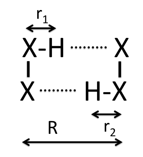
Figure 1: Definition of the key distances for a symmetrical system with two hydrogen bonds. $R$ is the distance between the donor and acceptor atoms involved in proton transfer. $r_{1}$ is the length of the upper X-H bond on the left molecule. The length of the lower X-H bond on the right molecule is $r_{2}$.

II A simple model for ground state potential energy surfaces

The four-state model proposed here builds on recent work concerning single hydrogen bonds and single proton transfer McKenzieCPL . A two diabatic state model with a simple parameterisation gives a ground state potential energy surface that can describe a wide range of experimental data (bond lengths, stretching and bending vibrational frequencies, and isotope effects) for a diverse set of molecular complexes, particularly when quantum nuclear motion is taken into account McKenzieJCP .

II.1 Reduced Hilbert space for the effective Hamiltonian

Diabatic states Domcke:1994 ; Hong:2006 ; Sidis:2007 ; VanVoorhis:2010 (including valence bond states) are a powerful tool for developing chemical concepts Shaik , including understanding and describing conical intersections Yarkony:1998 , and going beyond the Born-Oppenheimer approximation McKemmish . Previously it has been proposed that hydrogen bonding and hydrogen transfer reactions can be described by Empirical Valence Bond models Warshel:1991 where the diabatic states are valence bond states. In the model considered here, the reduced Hilbert space has a basis consisting of the four diabatic states shown in Figure 2. Each represents a product state of the electronic states of the left unit and the right unit, i.e, the state that would be an eigenstate as the distance $R\to\infty$. The difference between the two states $|A>$, $|B>$ and the two states $|L>$, $|R>$ is transfer of a single proton. Each of the diabatic states involves X-H bonds; they have both covalent and ionic contributions, the relative weight of which depends on the length of the X-H bond. A Morse potential is used to describe the energy of each of these bonds and thus the energy of the diabatic states (see below).

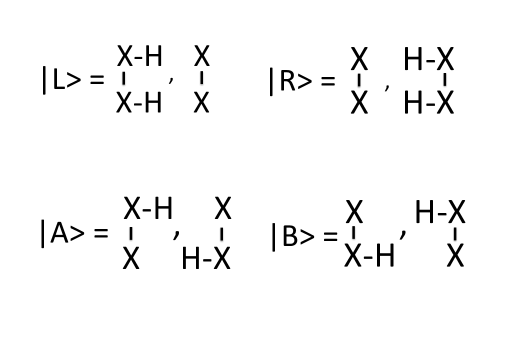
Figure 2: Four diabatic states. The top two states differ from the bottom two by transfer of a single proton, i.e., for the top two states both protons are on either the left molecule or the right molecule. A key parameter in the model is $D_{2}/D_{1}$, the ratio of the proton affinity in the top two states to that in the bottom two states.

In this paper I focus solely on the symmetric case where the donor and acceptor are symmetrical, i.e., the states $|A>$ and $|B>$ are degenerate with each other at their respective equilibrium bond lengths, as are the two states $|L>$ and $|R>$.

II.2 Effective Hamiltonian

The Hamiltonian for the four diabatic states has matrix elements that depend on the X-H bond lengths, $r_{1}$ and $r_{2}$, and the donor-acceptor separation $R$ (compare Figure 1). For simplicity, I assume the hydrogen bonds are linear. It is straightforward to also take into account non-linear bonds McKenzieCPL . The Morse potential describes the energy of a single X-H bond. The two cases $j=1,2$ denote the presence of one or two X-H bonds, respectively, within the left and right molecules shown in Figure 2. The Morse potential is

$$V_{j}(r)=D_{j}[\exp(-2a_{j}(r-r_{0j}))-2\exp(-a_{j}(r-r_{0j}))]$$ (1)

where $D_{j}$ is the binding energy, $r_{0j}$ is the equilibrium bond length, and $a_{j}$ is the decay constant. $D_{1}$ and $D_{2}$ denote the proton affinity, with one and two protons attached, respectively. Generally, I expect $D_{2}<D_{1}$, and actual values for their relative size for specific molecules are discussed later. The harmonic vibrational frequency $\omega$ of an isolated X-H bond is given by $\mu\omega^{2}=2D_{j}a_{j}^{2}$ where $\mu$ is the reduced mass of the proton. For O-H bonds approximate parameters are $\omega\simeq 3750$ cm^-1, $D\simeq 120$ kcal/mol, $a\simeq 2.2/\AA$, $r_{0}\simeq 0.96\ \AA$. I take $a_{1}=a_{2}$ and $r_{01}=r_{02}$.

The effective Hamiltonian describing the four interacting diabatic states is taken to have the form

$$H=\left(\begin{array}[]{cccc}V_{2}(r_{1})+V_{2}(R-r_{2})&0&\Delta(R)&\Delta(R)\\ 0&V_{2}(R-r_{1})+V_{2}(r_{2})&\Delta(R)&\Delta(R)\\ \Delta(R)&\Delta(R)&V_{1}(r_{1})+V_{1}(r_{2})&0\\ \Delta(R)&\Delta(R)&0&V_{1}(R-r_{1})+V_{1}(R-r_{2})\end{array}\right)$$ (2)

where the basis for the four-dimensional Hilbert space is taken in the order $|L>$, $|R>$, $|A>$, and $|B>$. The diabatic states that differ by one proton in number are coupled via the matrix element $\Delta(R)$. The coupling between states that differ by two protons is assumed to be negligibly small.

II.3 Parameterisation of the diabatic coupling $\Delta(R)$

The matrix element associated with proton transfer is assumed to have the simple form McKenzieCPL

$$\Delta(R)=\Delta_{1}\exp(-b(R-R_{1}))$$ (3)

and $b$ defines the decay rate of the matrix element with increasing $R$. $R_{1}$ is a reference distance defined as $R_{1}\equiv 2r_{0}+1/a\simeq 2.37\ \AA$. This distance is introduced so that the scale $\Delta_{1}$ is an energy scale that is physically relevant. There will be some variation in the parameters $\Delta_{1}$ and $b$ with the chemical identity of the atoms (e.g. O, N, S, Se, …) in the donor and acceptor that are directly involved in the H-bonds. Since the Morse potential parameters are those of isolated X-H bonds the model for a single hydrogen bond has essentially two free parameters, $b$, and $\Delta_{1}$. These respectively set the length and energy scales associated with the interaction between any two diabatic states that are related by transfer of a single proton. The parameter values that are used here, $\Delta_{1}=0.4D_{1}\simeq$ 48 kcal/mol and $b=2.2/\AA$ for O-H$\cdots$O systems, were estimated from comparisons of the predictions of the model with experiment McKenzieCPL , and give particularly good agreement when quantum nuclear effects are taken into account McKenzieJCP . Appropriate parameter values for N-H$\cdots$N bonds are discussed later.

II.4 Four different classes of ground state potential energy surfaces

In the adiabatic limit [i.e., the classical limit where the protons are taken to have infinite mass] the four electronic energy eigenvalues of the Hamiltonian (2) define potential energy surfaces (PES) for each of the four electronic states. I focus on the smallest eigenvalue, which describes the ground state potential surface $\epsilon_{0}(r_{1},r_{2},R)$. Figure 3 shows four qualitatively different ground state surfaces, depending on the value of the two parameters $R$ and $D_{2}/D_{1}$. The four different classes are now defined and discussed. The classes differ by the number of saddle points on the potential surface. The last three classes were delineated previously in Reference Smedarchina:2008, .

Class I. There is a single minimum and no local maxima on the surface. The two protons will be completely delocalised between the four different binding sites.

Class II. There are two local minima and a single saddle point equidistant between them. Double proton transfer will occur by the concerted mechanism. Both the minimum energy path (for activated transfer at high temperatures) and the instanton path associated with quantum tunneling (at low temperatures) is along the diagonal direction $r_{1}=r_{2}$.

Class III. There are two local minima and a single maxima equidistant between them, and two saddle points (transition states) on opposite sides of the maxima. Activated transfer will occur via either of the saddle points and thus can be described as a compromise between concerted and sequential transfer. Depending on the details there may be a single linear instanton path (concerted tunneling) or two non-linear paths on either side of the potential maximum (partially concerted tunneling) Benderskii:2003 .

Class VI. There are four local minima and a single maxima equidistant between them, and four saddle points (transition states). Activated transfer will occur via sequential transfer. The minimum energy path may involve a significant energy plateau [a “structureless transition state”] as found in some previous computational chemistry calculations for pyrazole-guanidine Schweiger-2003 .

Classes I, II, and III can be distinguished by examining the local curvature of the PES at the symmetric point $r_{1}=r_{2}=R/2$. In particular

$$K_{1}\equiv\left.\frac{\partial^{2}\epsilon_{0}(r,r,R)}{\partial r^{2}}\right|_{r=R/2}.$$ (4)

is positive for class I and negative for all the others. The curvature in the perpendicular direction

$$K_{2}\equiv\left.\frac{\partial^{2}\epsilon_{0}(r,R-r,R)}{\partial r^{2}}\right|_{r=R/2}$$ (5)

is positive for classes I and II and negative for classes III and IV. $K_{1}$ and $K_{2}$ are proportional to the vibrational frequencies $\omega_{s}$ and $\omega_{a}$, respectively, introduced in Ref. Smedarchina:2007, , and used there to distinguish classes II and III.

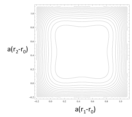
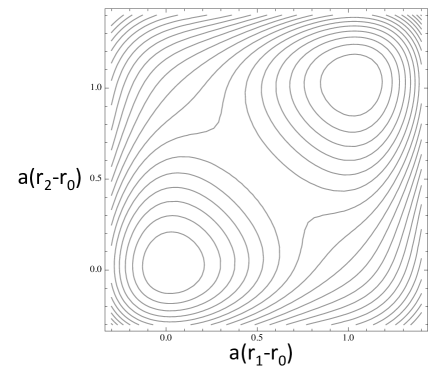
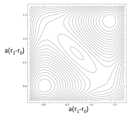
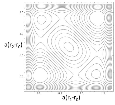
Figure 3: Representatives of the four different classes of two-dimensional ground state potential energy surfaces. Top left: Class I, no saddle point, $R=2.3\AA,D_{1}=D_{2}$. The contour level spacing is $0.007D_{1}=0.84$ kcal/mol. Top right: Class II, one saddle point, $R=2.4\AA,D_{2}/D_{1}=0.5$. The contour level spacing is $0.02D_{1}=2.4$ kcal/mol. Bottom left: Class III, two saddle points, $R=2.56\AA,D_{2}/D_{1}=0.7$. The contour level spacing is $0.018D_{1}=2.2$ kcal/mol. Bottom right: Class IV, four saddle points, $R=2.56\AA,D_{2}/D_{1}=0.9$. The contour level spacing is $0.015D_{1}=1.8$ kcal/mol. Parameters relevant to O-H $\cdots$O bonds, $r_{0}=0.96\AA$, $a=2.2/\AA$, and $D_{1}=120$ kcal/mol McKenzieCPL , were used.

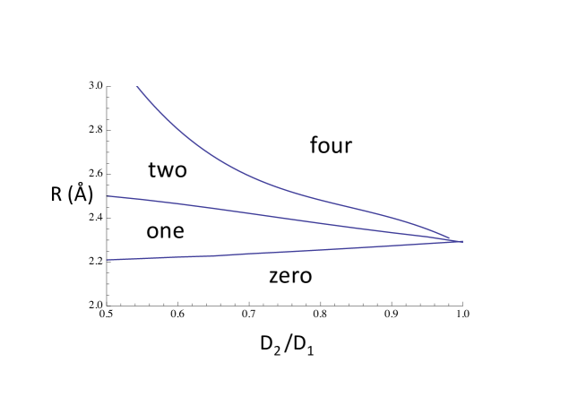
Figure 4: Phase diagram of the model as a function of the donor-acceptor distance $R$ and the ratio of the double to single proton affinities $D_{2}/D_{1}$. Parameter regions where the ground state potential energy surface has zero, one, two, or four saddle points are indicated. The vertical scale is for parameters appropriate for O-H$\cdots$O bonds. The $R$ values would be larger by approximately $0.14\AA$ for N-H$\cdots$N bonds.

Figure 4 shows the ”phase diagram” of the system as a function of the donor-acceptor distance $R$ and ratio of proton affinities, $D_{1}/D_{2}$, i.e., for which parameter regions the classes I-IV listed above occur. In particular, for fixed $D_{2}/D_{1}$ as $R$ decreases from a large value there will be a transition from class IV to III to II to I.

Catastrophe theory has been used to describe the qualitative changes in energy landscapes that occur with variation of a system parameter Wales:2003 . Examining the plots shown in Figure 3, suggests that the cusp catastrophe describes transitions between classes I and II and between II and III. The transition between III and IV is described by two simultaneous fold catastrophes.

If the extrema are isolated the relative number of minima ($N_{min}$), maxima ($N_{max}$), and saddle points ($N_{s}$) on the potential energy surface is constrained by the relation

$$N_{min}+N_{max}-N_{s}=1.$$ (6)

For example, in class IV, $4+1-4=1$. Hence, if varying the system parameters introduces an extra maxima or minima then one additional saddle point must also appear. This relation is a consequence of differential topology [Morse theory and the Poincare-Hopf index theorem]. The minima and maxima are associated with an index $+1$ and saddle points with $-1$, where the index is $(-1)^{J}$ with $J$ the number of negative eigenvalues of the Hessian matrix at the extremal point. A general theorem McKenzie83 states that if a smooth function $f(\vec{r})\to\infty$ as $|\vec{r}|\to\infty$ or if the gradient of $f$ points outward over a closed surface (curve in two dimensions), then the isolated extrema of $f$ inside that closed surface, must satisfy the relation (6). This condition is satisfied on general grounds because extreme compression or stretching of a bond makes the energy very large compared to the equilibrium energy. There have only been a few previous discussions about how global constraints such as equation (6) follow from differential topology. Mezey considered lower and upper bounds for $N_{min}$, $N_{max}$, and $N_{s}$, based on the Morse inequalities Mezey:1981 ; Mezey:1987 . Pick considered the corresponding equation [which has zero on the right hand side] for absorbates on periodic substrates Pick:2009 .

A study of a simple model two-dimensional potential for double proton transfer Benderskii:2003 also produced a phase diagram as a function of the model parameters and considered bifurcation of the instanton tunneling paths. However, it has been argued that the model potential used there does not respect some of the symmetries of the problem Smedarchina:2007 .

II.5 Co-operativity of hydrogen bonds

The ground state energy of the double H-bond system can be compared to that of two decoupled H-bonds where $D_{1}$ is the binding energy of an isolated X-H bond. The energy of a single H-bond for the corresponding two-diabatic state model McKenzieCPL is

$$\epsilon_{0}^{1}(R,r)={1\over 2}\left(V_{1}(r)+V_{1}(R-r)-\sqrt{(V_{1}(r)-V_{1}(R-r))^{2}+4\Delta(R)^{2}}\right)$$ (7)

and the ground state energy of the two decoupled H-bonds is

$$\epsilon_{0}(R,r_{1},r_{2})=\epsilon_{0}^{1}(R,r_{1})+\epsilon_{0}^{1}(R,r_{2}).$$ (8)

It turns out that for $D_{2}=D_{1}$ the ground state energy of the Hamiltonian (2) is given by an identical expression. Thus, we see that it is differences between the single and double proton affinities that couple the two H-bonds together. The question of whether the two bonds are co-operative or not is subtle. Is the binding energy enhanced or decreased? Is the barrier for double proton transfer increased or decreased? Figure 4 shows that as $D_{2}/D_{1}$ decreases (and thus the coupling between the two H-bonds increases) that the $R$ value needed to remove the barrier decreases. This is a signature of anti-co-operative behaviour. Similarly the barrier for concerted proton transfer increases as $D_{2}/D_{1}$ decreases.

III Model parameter values for specific molecules

The above analysis shows that a key parameter in the model is $D_{2}/D_{1}$, the ratio of the second proton affinity, $D_{2}$ to the first proton affinity, $D_{1}$. Unfortunately, there are few calculations or measurements of $D_{2}$ for specific molecules, that I am aware of. DFT-B3LYP and MP2 calculations for diazanaphthalenes give $D_{2}/D_{1}\simeq 0.5$ Spedaletti:2005 . DFT calculations for a series of diamines containing hydrocarbon bridges give $D_{2}/D_{1}\sim 0.8-0.9$ Bayat:2010 . For uracil, DFT-B3LYP calculations give a proton affinity of 800-900 kJ/mol depending on the protonation site and the tautomer, and a deprotonation enthalpy of 1350-1450 kJ/mol Kryachko . This is equivalent to $D_{2}/D_{1}\simeq 0.6-0.7$. For the chromophore of the Green fluorescent protein, the ground state energies of four different protonation states have been calculated at the level of MS-CASPT2 with a SA2-CAS(4,3) reference at the MP2 ground state geometry with a cc-pvdz basis set Olsen:2010 . With respect to the anion state the energies of the phenol, imidazolol, and oxonol cation states are -15.09, -13.74, and -24.72 eV, respectively. This leads to $D_{2}/D_{1}\simeq 0.7-0.8$. Given the values discussed above, the parameter range $0.5<D_{2}/D_{1}<1$ shown in Figure 4 is chemically realistic.

For porphycenes chemical substitutions external to the cavity produce a range of $R$ values for the N-H$\cdots$N bonds inside the cavity between 2.5 and 2.9 $\AA$ Waluk:2010 . This variation leads to the tautomerisation [double proton transfer] rate increasing smoothly by more than three orders of magnitude as $R$ decreases Fita:2009 . This is consistent with the fact that in the model presented here the scale of the energy barriers is largely determined by $V(R/2)-\Delta(R)$ which decreases with decreasing $R$.

The plots shown in this paper use a parameterisation for O-H$\cdots$O bonds McKenzieCPL . The parameterisation will be slightly different for N-H$\cdots$N bonds. For N-H bonds Warshel Warshel:1991 has Morse potential parameter values: $r_{0}=1.00\AA$, $a=2.07/\AA$, and $D=103$ kcal/mol, compared to values for O-H of $r_{0}=0.96\AA$, $a=2.26/\AA$, and $D=102$ kcal/mol. These differences will increase the $R$ values on the vertical scale of Figure 4 by approximately $0.14\AA$, assuming the same parameterisation of $\Delta(R)$, i.e., $b=a$ and $\Delta_{1}=0.4D$.

For single hydrogen bonds, with symmetric donor and acceptor, empirical correlations between $R$ and a range of observables such as bond lengths, vibrational frequencies, NMR chemical shifts, and geometric isotope effects are observed Gilli ; McKenzieCPL ; McKenzieJCP . Our model suggests that for systems with double hydrogen bonds such correlations will only occur for systems with identical values of the parameter $D_{2}/D_{1}$. For carboxylic acid dimers it was found that $R$ coud be varied systematically by enclosing them in a molecular capsule Ajami:2011 . Families of porphycenes Waluk:2010 may also be appropriate systems to investigate such correlations.

An important task is to determine in which of the four classes specific molecular systems belong. The formic acid dimer is the simplest dimer of carboxylic acids. A tunnel splitting of $2.86\times 10^{-3}$ cm^-1 for the C=O stretch mode has been observed at low temperatures Madeja:2002 and identified with a tunneling path associated with concerted transfer. A transition from class II to III with increasing $R$ was observed in quantum chemistry calculations for the formic acid dimer. Shida et al. Shida:1991 found a transition from one to two saddle points when $R\simeq 2.7\AA$. Smedarchina et al.Smedarchina:2008 found a transition for $R=2.56\AA$. In the simple model considered hear the transition occurs for $R\simeq 2.4\AA$. The experimental value for the equilibrium bond length is $R=2.696\AA$ from electron diffraction, compared to the value of $R=2.72\AA$ based on DFT calculations Smedarchina:2008 suggesting that formic acid is in class III.

An interesting question is whether there are any compounds that fall in class I, i.e., with completely delocalised protons. For N-H$\cdots$H bonds this will require $R<2.35\AA$, which is fairly unlikely. However, the quantum zero-point motion of the protons may lead to delocalisation at larger distances, $R\simeq 2.5\AA$, provided that the energy barrier is less than the zero-point vibrational energy McKenzieJCP .

IV Conclusions

A simple model has been introduced that can describe four different classes of potential energy surfaces for double proton transfer in symmetric hydrogen-bonded complexes, such as porphycenes and carboxylic acid dimers. The model is based on a chemically and physically transparent effective Hamiltonian involving four diabatic states. The number of saddle points on the ground state potential energy surface is determined by the value of two different parameters: $R$, the distance between the donor and acceptor atoms for proton transfer, and $D_{2}/D_{1}$, the ratio of the proton affinity of a donor with two and one protons attached. Double proton transfer will occur via a concerted, partially concerted, or sequential mechanism depending on the class of potential energy surface involved.

- (1) Agostino Migliore, Nicholas F. Polizzi, Michael J. Therien, and David N. Beratan. Chemical Reviews, 114: 3381–3465, 2014.
- (2) Jacek Waluk. Accounts of Chemical Research, 39:945–952, 2006.
- (3) Jacek Waluk. Handbook of Porphyrin Science, chapter 4, pages 359–435. World Scientific. Singapore. 2010.
- (4) Sylwester Gawinkowski, Lukasz Walewski, Alexander Vdovin, Alkwin Slenczka, Stephane Rols, Mark R Johnson, Bogdan Lesyng, and Jacek Waluk. Phys. Chem. Chem. Phys., 14:5489–5503, 2012.
- (5) Oh-Hoon Kwon and Ahmed Zewail. Proceedings of the National Academy of Sciences, 104:8703–8708, 2007.
- (6) Zorka Smedarchina, Willem Siebrand, and Antonio Fernández-Ramos. The Journal of Chemical Physics, 127:174513, 2007.
- (7) Zorka Smedarchina, Willem Siebrand, Antonio Fernández-Ramos, and Ruben Meana-Paneda. Zeitschrift für Physikalische Chemie, 222:1291, 2008.
- (8) Ross H. McKenzie. Chemical Physics Letters, 535:196 – 200, 2012.
- (9) Ross H. McKenzie, Christiaan Bekker, Bijyalaxmi Athokpam, and Sai G. Ramesh. The Journal of Chemical Physics, 140:174508, 2014.
- (10) W Domcke, C Woywod, and M Stengle. Chemical Physics Letters, 226:257–262, 1994.
- (11) Gongyi Hong, Edina Rosta, and Arieh Warshel. The Journal of Physical Chemistry B, 110:19570–19574, 2006.
- (12) V Sidis. Advances in Chemical Physics, 87:73–134, 1992.
- (13) Troy Van Voorhis, Tim Kowalczyk, Benjamin Kaduk, Lee-Ping Wang, Chiao-Lun Cheng, and Qin Wu. Annual Review of Physical Chemistry, 61:149–170, 2010.
- (14) S.S. Shaik and P.C. Hiberty. A Chemists Guide to Valence Bond Theory. Wiley, New York, 2007.
- (15) David R Yarkony. Accounts of chemical research, 31:511–518, 1998.
- (16) Laura K. McKemmish, Ross H. McKenzie, Noel S. Hush, and Jeffrey R. Reimers. The Journal of Chemical Physics, 135:244110, 2011.
- (17) Arieh Warshel. Computer modeling of chemical reactions in enzymes and solutions. Wiley, New York, 1991.
- (18) V. A. Benderskii, E. V. Vetoshkin, E. I. Kats, and H. P. Trommsdorff. Phys. Rev. E, 67:026102, 2003.
- (19) Stefan Schweiger and Guntram Rauhut. The Journal of Physical Chemistry A, 107:9668–9678, 2003.
- (20) David Wales. Energy landscapes: Applications to clusters, biomolecules and glasses. Cambridge University Press, Cambridge, 2003.
- (21) Ross H. McKenzie. Journal of the Australian Mathematical Society (Series A), 37:413–415, 1984.
- (22) Paul G Mezey. Chemical Physics Letters, 82:100–104, 1981.
- (23) Paul G Mezey. Potential energy hypersurfaces. Elsevier, New York, 1987.
- (24) S. Pick. Phys. Rev. B, 79:045403, 2009.
- (25) César A. Spedaletti, Mario R. Estrada, Graciela N. Zamarbide, Juan C. Garro, Carlos A. Ponce, and Francisco Tomas Vert. Journal of Molecular Structure: THEOCHEM, 719:115 – 118, 2005.
- (26) Mehdi Bayat and Sadegh Salehzadeh. Journal of Molecular Structure: THEOCHEM, 957:120 – 125, 2010.
- (27) Eugene S. Kryachko, Minh Tho Nguyen, and Therese Zeegers-Huyskens. The Journal of Physical Chemistry A, 105:1288–1295, 2001.
- (28) Seth Olsen. Journal of Chemical Theory and Computation, 6:1089–1103, 2010.
- (29) P. Fita, N. Urbańska, C. Radzewicz, and J. Waluk. Chemistry – A European Journal, 15:4851–4856, 2009.
- (30) G. Gilli and P. Gilli. The Nature of the Hydrogen Bond. Oxford U.P., Oxford, 2009.
- (31) D. Ajami, P.M. Tolstoy, H. Dube, S. Odermatt, B. Koeppe, J. Guo, H.-H. Limbach, and J. Rebek, Angewandte Chemie International Edition, 50:1521-3773, 2011.
- (32) F. Madeja and M. Havenith. The Journal of Chemical Physics, 117:7162–7168, 2002.
- (33) Norihiro Shida, Paul F Barbara, and Jan Almlöf. The Journal of Chemical Physics, 94:3633–3643, 1991.