Remarkable optics of short-pitch deformed helix ferroelectric liquid crystals: symmetries, exceptional points and polarization-resolved angular patterns

Abstract

In order to explore electric-field-induced transformations of polarization singularities in the polarization-resolved angular (conoscopic) patterns emerging after deformed helix ferroelectric liquid crystal (DHFLC) cells with subwavelength helix pitch, we combine the transfer matrix formalism with the results for the effective dielectric tensor of biaxial FLCs evaluated using an improved technique of averaging over distorted helical structures. Within the framework of the transfer matrix method, we deduce a number of symmetry relations and show that the symmetry axis of $L$ lines (curves of linear polarization) is directed along the major in-plane optical axis which rotates under the action of the electric field. When the angle between this axis and the polarization plane of incident linearly polarized light is above its critical value, the $C$ points (points of circular polarization) appear in the form of symmetrically arranged chains of densely packed star-monstar pairs. We also emphasize the role of phase singularities of a different kind and discuss the enhanced electro-optic response of DHFLCs near the exceptional point where the condition of zero-field isotropy is fulfilled.

I Introduction

Over the last more than three decades ferroelectric liquid crystals (FLCs) have attracted considerable attention as promising chiral liquid crystal materials for applications in fast switching display devices (a detailed description of FLCs can be found, e.g., in monographs Lagerwall (1999); Oswald and Pieranski (2006)). Equilibrium orientational structures in FLCs are represented by helical twisting patterns where FLC molecules align on average along a local unit director

$$\hat{\mathbf{d}}=\cos\theta\,\hat{\mathbf{h}}+\sin\theta\,\hat{\mathbf{c}},$$ (1)

where $\theta$ is the smectic tilt angle; $\hat{\mathbf{h}}$ is the twisting axis normal to the smectic layers and $\hat{\mathbf{c}}\perp\hat{\mathbf{h}}$ is the $c$-director. The FLC director (1) lies on the smectic cone depicted in Fig. 1a with the smectic tilt angle $\theta$ and rotates in a helical fashion about a uniform twisting axis $\hat{\mathbf{h}}$ forming the FLC helix with the helix pitch, $P$. This rotation is described by the azimuthal angle around the cone $\Phi$ that specifies orientation of the $c$-director in the plane perpendicular to $\hat{\mathbf{h}}$ and depends on the dimensionless coordinate along the twisting axis

$$\phi=2\pi\bigl{(}{\hat{\mathbf{h}}}\cdot{\mathbf{r}}\bigr{)}/P=qx,$$ (2)

where $q=2\pi/P$ is the helix twist wave number.

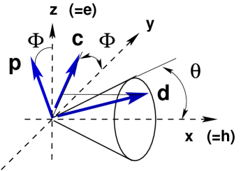
(a) Smectic cone

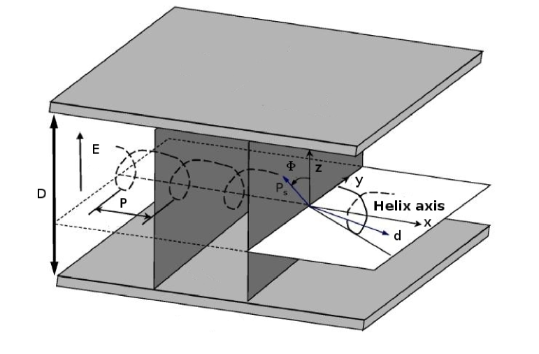
(b) Planar aligned FLC cell

Figure 1: (Color online) Geometry of (a) smectic cone and (b) planar aligned FLC cell with uniform lying helix.

The important case of a uniform lying FLC helix in the slab geometry with the smectic layers normal to the substrates and

$$\hat{\mathbf{h}}=\hat{\mathbf{x}},\quad\hat{\mathbf{c}}=\cos\Phi\,\hat{\mathbf{y}}+\sin\Phi\,\hat{\mathbf{z}},\quad\mathbf{E}=E\,\hat{\mathbf{z}},$$ (3)

where $\mathbf{E}$ is the electric field applied across the cell, is illustrated in Fig. 1. This is the geometry of surface stabilized FLCs (SSFLCs) pioneered by Clark and Lagerwall in Clark and Lagerwall (1980). They studied electro-optic response of FLC cells confined between two parallel plates subject to homogeneous boundary conditions and made thin enough to suppress the bulk FLC helix.

It was found that such cells exhibit high-speed, bistable electro-optical switching between orientational states stabilized by surface interactions. The response of FLCs to an applied electric field $\mathbf{E}$ is characterized by fast switching times due to linear coupling between the field and the spontaneous ferroelectric polarization

$$\mathbf{P}_{s}=P_{s}\hat{\mathbf{p}},\quad\hat{\mathbf{p}}=\hat{\mathbf{h}}\times\hat{\mathbf{c}}=\cos\Phi\,\hat{\mathbf{z}}-\sin\Phi\,\hat{\mathbf{y}},$$ (4)

where $\hat{\mathbf{p}}$ is the polarization unit vector. There is also a threshold voltage necessary for switching to occur and the process of bistable switching is typically accompanied by a hysteresis.

Figure 1b also describes the geometry of deformed helix FLCs (DHFLCs) as it was introduced in Beresnev et al. (1989). This case will be of our primary concern.

In DHFLC cells, the FLC helix is characterized by a short submicron helix pitch, $P<1$ $\mu$m, and a relatively large tilt angle, $\theta>30$ deg. By contrast to SSFLC cells, where the surface induced unwinding of the bulk helix requires the helix pitch of a FLC mixture to be greater than the cell thickness, a DHFLC helix pitch is 5-10 times smaller than the thickness. This allows the helix to be retained within the cell boundaries.

Electro-optical response of DHFLC cells exhibits a number of peculiarities that make them useful for LC devices such as high speed spatial light modulators Abdulhalim and Moddel (1991); Cohen et al. (1997); Pozhidaev et al. (2000, 2013, 2014), colour-sequential liquid crystal display cells Hedge et al. (2008) and optic fiber sensors Brodzeli et al. (2012). The effects caused by electric-field-induced distortions of the helical structure underline the mode of operation of such cells. In a typical experimental setup, these effects are probed by performing measurements of the transmittance of normally incident linearly polarized light through a cell placed between crossed polarizers.

A more general case of oblique incidence has not received a fair amount of attention. Theoretically, a powerful tool to deal with this case is the transfer matrix method which has been widely used in studies of both quantum mechanical and optical wave fields Markoš and Soukoulis (2008); Yariv and Yeh (2007). In this work we apply the method for systematic treatment of the technologically important case of DHFLCs with subwavelength pitch also known as the short-pitch DHFLCs.

Recently, the transfer matrix approach to polarization gratings was employed to define the effective dielectric tensor of short-pitch DHFLCs Kiselev et al. (2011) that gives the principal values and orientation of the optical axes as a function of the applied electric field. Biaxial anisotropy and rotation of the in-plane optical axes produced by the electric field can be interpreted as the orientational Kerr effect Pozhidaev et al. (2013, 2014).

It can be expected that the electric field dependence of the effective dielectric tensor will also manifest itself as electric-field-induced transformations of the polarization-resolved angular (conoscopic) patterns in the observation plane after the DHFLC cells illuminated by convergent light beam. These patterns are represented by the two-dimensional (2D) fields of polarization ellipses describing the polarization structure behind the conoscopic images Kiselev (2007a); Kiselev et al. (2008).

As it was originally recognized by Nye Nye (1983); Nye and Hajnal (1987); Nye (1999), the key elements characterizing geometry of such Stokes parameter fields are the polarization singularities that play the fundamentally important role of structurally stable topological defects (a recent review can be found in Ref. Dennis et al. (2009)). In particular, the polarization singularities such as the C points (the points where the light wave is circular polarized) and the L lines (the curves along which the polarization is linear) frequently emerge as the characteristic feature of certain polarization state distributions. For nematic and cholescteric (chiral nematic) liquid crystals, the singularity structure of the polarization-resolved angular patterns is generally found to be sensitive to both the director configuration and the polarization characteristics of incident light Kiselev (2007a); Kiselev et al. (2008); Egorov and Kiselev (2010).

In this study, we consider the polarization-resolved angular patterns of DHFLC cells as the Stokes parameter fields giving detailed information on the incidence angles dependence of the polarization state of light transmitted through the cells. In particular, we explore how the polarization singularities transform under the action of the electric field. Our analysis will utilize the transfer matrix approach in combination with the results for the effective dielectric tensor of biaxial FLCs evaluated using an improved technique of averaging over distorted helical structures. We also emphasize the role of phase singularities of a different kind and discuss the electro-optic behavior of DHFLCs near the exceptional point where the condition of zero-field isotropy is fulfilled.

The layout of the paper is as follows. In Sec. II we introduce our notations and describe the transfer matrix formalism rendered into the $4\times 4$ matrix form suitable for our purposes. This formalism is employed to deduce a number of the unitarity and symmetry relations with emphasis on the planar anisotropic structures that represent DHFLC cells and posses two optical axes lying in the plane of substrates. In Sec. III we evaluate the effective dielectric tensor of DHFLC cells, discuss the orientational Kerr effect and show that electro-optic response of DHFLC cells is enhanced near the exceptional point determined by the condition of zero-field isotropy. Geometry of the polarization-resolved angular patterns emerging after DHFLC cells is considered in Sec. IV. After providing necessary details on our computational approach and the polarization singularities, we present the numerical results describing how the singularity structure of polarization ellipse fields transforms under the action of the electric field. Finally, in Sec. V we draw the results together and make some concluding remarks. Details on some technical results are relegated to Appendixes A–C.

Figure 2: Four-wave geometry with two incoming (incident) waves, $\mathbf{E}_{\mathrm{in}}^{(+)}$ and $\mathbf{E}_{\mathrm{in}}^{(-)}$, impinging onto the entrance ($z=0$) and exit ($z=D$) faces, respectively.

II Transfer matrix method and symmetries

In order to describe both the electro-optical properties and the polarization-resolved angular patterns of deformed helix ferroelectric liquid crystal layers with subwavelength pitch we adapt a general theoretical approach which can be regarded as a modified version of the well-known transfer matrix method Markoš and Soukoulis (2008); Yariv and Yeh (2007) and was previously applied to study the polarization-resolved conoscopic patterns of nematic liquid crystal cells Kiselev (2007a); Kiselev et al. (2008); Kiselev and Vovk (2010). This approach has also been extended to the case of polarization gratings and used to deduce the general expression for the effective dielectric tensor of DHFLC cells Kiselev et al. (2011).

In this section, we present the transfer matrix approach as the starting point of our theoretical considerations, with emphasis on its general structure and the symmetry relations. The analytical results for uniformly anisotropic planar structures representing homogenized DHFLC cells are given in Appendix B.

We deal with a harmonic electromagnetic field characterized by the free-space wave number $k_{\mathrm{vac}}=\omega/c$, where $\omega$ is the frequency (time-dependent factor is $\exp\{-\omega t\}$), and consider the slab geometry shown in Fig. 2. In this geometry, an optically anisotropic layer of thickness $D$ is sandwiched between the bounding surfaces (substrates): $z=0$ and $z=D$ (the $z$ axis is normal to the substrates) and is characterized by the dielectric tensor $\epsilon_{ij}$ and the magnetic permittivity $\mu$

Further, we restrict ourselves to the case of stratified media and assume that the electromagnetic fields can be taken in the following factorized form

$$\{\mathbf{E}(\mathbf{r}),\mathbf{H}(\mathbf{r})\}=\{\mathbf{E}(z),\mathbf{H}(z)\}\exp\bigl{(}{\mathbf{k}_{p}}\cdot{\mathbf{r}}\bigr{)},$$ (5)

where the vector

$$\mathbf{k}_{p}/k_{\mathrm{vac}}=\mathbf{q}_{p}=(q_{x}^{(p)},q_{y}^{(p)},0)=q_{p}(\cos\phi_{p},\sin\phi_{p},0)$$ (6)

represents the lateral component of the wave vector. Then we write down the representation for the electric and magnetic fields, $\mathbf{E}$ and $\mathbf{H}$,

$$\mathbf{E}=E_{z}\hat{\mathbf{z}}+\mathbf{E}_{P},\quad\mathbf{H}=H_{z}\hat{\mathbf{z}}+\hat{\mathbf{z}}\times\mathbf{H}_{P},$$ (7)

where the components directed along the normal to the bounding surface (the $z$ axis) are separated from the tangential (lateral) ones. In this representation, the vectors $\mathbf{E}_{P}=E_{x}\hat{\mathbf{x}}+E_{y}\hat{\mathbf{y}}\equiv\begin{pmatrix}E_{x}\\ E_{y}\end{pmatrix}$ and $\mathbf{H}_{P}=\mathbf{H}\times\hat{\mathbf{z}}\equiv\begin{pmatrix}H_{y}\\ -H_{x}\end{pmatrix}$ are parallel to the substrates and give the lateral components of the electromagnetic field.

Substituting the relations (7) into the Maxwell equations and eliminating the $z$ components of the electric and magnetic fields gives equations for the tangential components of the electromagnetic field that can be written in the following $4\times 4$ matrix form Kiselev et al. (2008, 2011):

$$-i\partial_{\tau}\mathbf{F}=\mathbf{M}\cdot\mathbf{F}\equiv\begin{pmatrix}\mathbf{M}_{11}&\mathbf{M}_{12}\\ \mathbf{M}_{21}&\mathbf{M}_{22}\end{pmatrix}\begin{pmatrix}\mathbf{E}_{P}\\ \mathbf{H}_{P}\end{pmatrix},\quad\tau\equiv k_{\mathrm{vac}}z,$$ (8)

where $\mathbf{M}$ is the differential propagation matrix and its $2\times 2$ block matrices $\mathbf{M}_{ij}$ are given by

$$\mathbf{M}^{(11)}_{\alpha\beta}=-\epsilon_{zz}^{-1}q_{\alpha}^{(p)}\epsilon_{z\beta},\quad\mathbf{M}^{(22)}_{\alpha\beta}=-\epsilon_{zz}^{-1}\epsilon_{\alpha z}q_{\beta}^{(p)},$$ (9a)

$$\mathbf{M}^{(12)}_{\alpha\beta}=\mu\delta_{\alpha\beta}-q_{\alpha}^{(p)}\,\epsilon_{zz}^{-1}\,q_{\beta}^{(p)},$$ (9b)

$$\mathbf{M}^{(21)}_{\alpha\beta}=\epsilon_{\alpha\beta}-\epsilon_{\alpha z}\epsilon_{zz}^{-1}\epsilon_{z\beta}-\mu^{-1}p_{\alpha}^{(p)}p_{\beta}^{(p)},\quad\mathbf{p}_{p}=\hat{\mathbf{z}}\times\mathbf{q}_{p}.$$ (9c)

General solution of the system (8)

$$\mathbf{F}(\tau)=\mathbf{U}(\tau,\tau_{0})\cdot\mathbf{F}(\tau_{0})$$ (10)

can be conveniently expressed in terms of the evolution operator which is also known as the propagator and is defined as the matrix solution of the initial value problem

$$-i\partial_{\tau}\mathbf{U}(\tau,\tau_{0}) =\mathbf{M}(\tau)\cdot\mathbf{U}(\tau,\tau_{0}),$$ (11a)

$$\mathbf{U}(\tau_{0},\tau_{0}) =\mathbf{I}_{4},$$ (11b)

where $\mathbf{I}_{n}$ is the $n\times n$ identity matrix. Basic properties of the evolution operator are reviewed in Appendix A.

II.1 Input-output relations

In the ambient medium with $\epsilon_{ij}=\epsilon_{\mathrm{m}}\delta_{ij}$ and $\mu=\mu_{\mathrm{m}}$, the general solution (10) can be expressed in terms of plane waves propagating along the wave vectors with the tangential component (6). For such waves, the result is given by

$$\mathbf{F}_{\mathrm{m}}(\tau)=\mathbf{V}_{\mathrm{m}}(\mathbf{q}_{p})\begin{pmatrix}\exp\{i\mathbf{Q}_{\mathrm{m}}\,\tau\}&\mathbf{0}\\ \mathbf{0}&\exp\{-i\mathbf{Q}_{\mathrm{m}}\,\tau\}\end{pmatrix}\begin{pmatrix}\mathbf{E}_{+}\\ \mathbf{E}_{-}\end{pmatrix},$$ (12)

$$\mathbf{Q}_{\mathrm{m}}=q_{\mathrm{m}}\,\mathbf{I}_{2},\quad q_{\mathrm{m}}=\sqrt{n_{\mathrm{m}}^{2}-q_{p}^{2}},$$ (13)

where $\mathbf{V}_{\mathrm{m}}(\mathbf{q}_{n})$ is the eigenvector matrix for the ambient medium given by

$$\mathbf{V}_{\mathrm{m}}(\mathbf{q}_{p})=\mathbf{T}_{\mathrm{rot}}(\phi_{p})\mathbf{V}_{\mathrm{m}}=\begin{pmatrix}\mathbf{Rt}(\phi_{p})&\mathbf{0}\\ \mathbf{0}&\mathbf{Rt}(\phi_{p})\end{pmatrix}\begin{pmatrix}\mathbf{E}_{\mathrm{m}}&-\boldsymbol{\sigma}_{3}\mathbf{E}_{\mathrm{m}}\\ \mathbf{H}_{\mathrm{m}}&\boldsymbol{\sigma}_{3}\mathbf{H}_{\mathrm{m}}\\ \end{pmatrix},$$ (14)

$$\mathbf{E}_{\mathrm{m}}=\begin{pmatrix}q_{\mathrm{m}}/n_{\mathrm{m}}&0\\ 0&1\end{pmatrix},\quad\mu_{\mathrm{m}}\,\mathbf{H}_{\mathrm{m}}=\begin{pmatrix}n_{\mathrm{m}}&0\\ 0&q_{\mathrm{m}}\end{pmatrix},$$ (15)

$$\mathbf{Rt}(\phi)=\begin{pmatrix}\cos\phi&-\sin\phi\\ \sin\phi&\cos\phi\end{pmatrix},$$ (16)

$\{\boldsymbol{\sigma}_{1},\boldsymbol{\sigma}_{2},\boldsymbol{\sigma}_{3}\}$ are the Pauli matrices

$$\boldsymbol{\sigma}_{1}=\begin{pmatrix}0&1\\ 1&0\end{pmatrix},\>\boldsymbol{\sigma}_{2}=\begin{pmatrix}0&-i\\ i&0\end{pmatrix},\>\boldsymbol{\sigma}_{3}=\begin{pmatrix}1&0\\ 0&-1\end{pmatrix}.$$ (17)

From Eq. (12), the vector amplitudes $\mathbf{E}_{+}$ and $\mathbf{E}_{-}$ correspond to the forward and backward eigenwaves with $\mathbf{k}_{+}=k_{\mathrm{vac}}(q_{\mathrm{m}}\,\hat{\mathbf{z}}+\mathbf{q}_{p})$ and $\mathbf{k}_{-}=k_{\mathrm{vac}}(-q_{\mathrm{m}}\,\hat{\mathbf{z}}+\mathbf{q}_{p})$, respectively. Figure 2 shows that, in the half space $z\leq 0$ before the entrance face of the layer $z=0$, these eigenwaves describe the incoming and outgoing waves

$$\mathbf{E}_{+}|_{z\leq 0}=\mathbf{E}_{\mathrm{in}}^{(+)},\quad\mathbf{E}_{-}|_{z\leq 0}=\mathbf{E}_{\mathrm{out}}^{(+)},$$ (18)

whereas, in the half space $z\geq D$ after the exit face of the layer, these waves are given by

$$\mathbf{E}_{+}|_{z\geq D}=\mathbf{E}_{\mathrm{out}}^{(-)},\quad\mathbf{E}_{-}|_{z\geq D}=\mathbf{E}_{\mathrm{in}}^{(-)}.$$ (19)

In this geometry, there are two plane waves, $\mathbf{E}_{\mathrm{in}}^{(+)}$ and $\mathbf{E}_{\mathrm{in}}^{(-)}$, incident on the bounding surfaces of the anisotropic layer, $z=0$ and $z=D$, respectively. Then the standard linear input-output relations

$$\mathbf{E}_{\mathrm{trm}}=\mathbf{T}\mathbf{E}_{\mathrm{inc}},\quad\mathbf{E}_{\mathrm{refl}}=\mathbf{R}\mathbf{E}_{\mathrm{inc}}$$ (20)

linking the vector amplitudes of transmitted and reflected waves, $\mathbf{E}_{\mathrm{trm}}$ and $\mathbf{E}_{\mathrm{refl}}$ with the amplitude of the incident wave, $\mathbf{E}_{\mathrm{inc}}$ through the transmission and reflection matrices, $\mathbf{T}$ and $\mathbf{R}$, assume the following generalized form:

$$\begin{pmatrix}\mathbf{E}_{\mathrm{out}}^{(-)}\\ \mathbf{E}_{\mathrm{out}}^{(+)}\end{pmatrix}=\mathbf{S}\begin{pmatrix}\mathbf{E}_{\mathrm{in}}^{(+)}\\ \mathbf{E}_{\mathrm{in}}^{(-)}\end{pmatrix}=\begin{pmatrix}\mathbf{T}_{+}&\mathbf{R}_{-}\\ \mathbf{R}_{+}&\mathbf{T}_{-}\end{pmatrix}\begin{pmatrix}\mathbf{E}_{\mathrm{in}}^{(+)}\\ \mathbf{E}_{\mathrm{in}}^{(-)}\end{pmatrix},$$ (21)

where $\mathbf{S}$ is the matrix —  the so-called scattering matrix — that relates the outgoing and incoming waves; $\mathbf{T}_{+}$ ($\mathbf{R}_{+}$) is the transmission (reflection) matrix for the case when the incident wave is incoming from the half space $z\leq 0$ bounded by the entrance face, whereas the mirror symmetric case where the incident wave is impinging onto the exit face of the sample is described by the transmission (reflection) matrix $\mathbf{T}_{-}$ ($\mathbf{R}_{-}$). So, we have

$$\mathbf{T}=\mathbf{T}_{\pm},\quad\mathbf{R}=\mathbf{R}_{\pm},$$ (22a)

$$\mathbf{E}_{\mathrm{in}}^{(\pm)}=\mathbf{E}_{\mathrm{inc}}=\begin{pmatrix}E_{p}^{(\mathrm{inc})}\\ E_{s}^{(\mathrm{inc})}\end{pmatrix},\quad\mathbf{E}_{\mathrm{in}}^{(\mp)}=0,$$ (22b)

$$\mathbf{E}_{\mathrm{out}}^{(\pm)}=\mathbf{E}_{\mathrm{refl}}\equiv\begin{pmatrix}E_{p}^{(\mathrm{refl})}\\ E_{s}^{(\mathrm{refl})}\end{pmatrix},\quad\mathbf{E}_{\mathrm{out}}^{(\mp)}=\mathbf{E}_{\mathrm{trm}}\equiv\begin{pmatrix}E_{p}^{(\mathrm{trm})}\\ E_{s}^{(\mathrm{trm})}\end{pmatrix}.$$ (22c)

It is our task now to relate these matrices and the evolution operator given by Eq. (11). To this end, we use the boundary conditions requiring the tangential components of the electric and magnetic fields to be continuous at the boundary surfaces: $\mathbf{F}(0)=\mathbf{F}_{\mathrm{m}}(0-0)$ and $\mathbf{F}(h)=\mathbf{F}_{\mathrm{m}}(h+0)$, and apply the relation (11) to the anisotropic layer of the thickness $D$ to yield the following result

$$\mathbf{F}_{\mathrm{m}}(h+0)=\mathbf{U}(h,0)\cdot\mathbf{F}_{\mathrm{m}}(0-0),\quad h=k_{\mathrm{vac}}D.$$ (23)

II.2 Transfer matrix

On substituting Eqs. (12) into Eq. (23) we have

$$\begin{pmatrix}\mathbf{E}_{\mathrm{in}}^{(+)}\\ \mathbf{E}_{\mathrm{out}}^{(+)}\end{pmatrix}=\mathbf{W}\cdot\begin{pmatrix}\mathbf{E}_{\mathrm{out}}^{(-)}\\ \mathbf{E}_{\mathrm{in}}^{(-)}\end{pmatrix}$$ (24)

where the matrix $\mathbf{W}$ linking the electric field vector amplitudes of the waves in the half spaces $z<0$ and $z>D$ bounded by the faces of the layer will be referred to as the transfer (linking) matrix. The expression for the transfer matrix is as follows

$$\mathbf{W}=\mathbf{V}_{\mathrm{m}}^{-1}\cdot\mathbf{U}_{R}^{-1}(h)\cdot\mathbf{V}_{\mathrm{m}}=\begin{pmatrix}\mathbf{W}_{11}&\mathbf{W}_{12}\\ \mathbf{W}_{21}&\mathbf{W}_{22}\end{pmatrix}$$ (25)

where $\mathbf{U}_{R}(\tau)=\mathbf{T}_{\mathrm{rot}}(-\phi_{p})\mathbf{U}(\tau,0)\mathbf{T}_{\mathrm{rot}}(\phi_{p})$ is the rotated operator of evolution. This operator is the solution of the initial value problem (11) with $\mathbf{M}(\tau)$ replaced with $\mathbf{M}_{R}(\tau)=\mathbf{T}_{\mathrm{rot}}(-\phi_{p})\mathbf{M}(\tau)\mathbf{T}_{\mathrm{rot}}(\phi_{p})$.

From Eqs. (21) and (24), the block structure of the transfer matrix can be expressed in terms of the transmission and reflection matrices as follows

$$\mathbf{W}_{11}=\mathbf{T}_{+}^{-1},\quad\mathbf{W}_{12}=-\mathbf{T}_{+}^{-1}\cdot\mathbf{R}_{-},$$

$$\mathbf{W}_{21}=\mathbf{R}_{+}\cdot\mathbf{T}_{+}^{-1},\quad\mathbf{W}_{22}=\mathbf{T}_{-}-\mathbf{R}_{+}\cdot\mathbf{T}_{+}^{-1}\cdot\mathbf{R}_{-}.$$ (26)

Similarly, for inverse of the transfer matrix,

$$\mathbf{W}^{-1}=\begin{pmatrix}\mathbf{W}_{11}^{(-1)}&\mathbf{W}_{12}^{(-1)}\\ \mathbf{W}_{21}^{(-1)}&\mathbf{W}_{22}^{(-1)}\end{pmatrix},$$ (27)

we have

$$\mathbf{W}_{11}^{(-1)}=\mathbf{T}_{+}-\mathbf{R}_{-}\cdot\mathbf{T}_{-}^{-1}\cdot\mathbf{R}_{+},\quad\mathbf{W}_{12}^{(-1)}=\mathbf{R}_{-}\cdot\mathbf{T}_{-}^{-1},$$

$$\mathbf{W}_{21}^{(-1)}=-\mathbf{T}_{-}^{-1}\cdot\mathbf{R}_{+},\quad\mathbf{W}_{22}^{(-1)}=\mathbf{T}_{-}^{-1}.$$ (28)

II.3 Symmetries

In Appendix A, it is shown that, for non-absorbing media with symmetric dielectric tensor, $\epsilon_{ij}=\epsilon_{ji}$, the operator of evolution satisfies the unitarity relation (95). By using Eq. (95) in combination with the algebraic identity

$${\mathbf{V}}^{T}_{\mathrm{m}}\cdot\mathbf{G}\cdot\mathbf{V}_{\mathrm{m}}=N_{\mathrm{m}}\mathbf{G}_{3},$$ (29a)

$$\mathbf{G}=\begin{pmatrix}\mathbf{0}&\mathbf{I}_{2}\\ \mathbf{I}_{2}&\mathbf{0}\end{pmatrix},\quad\mathbf{G}_{3}=\mathop{\rm diag}\nolimits(\mathbf{I}_{2},-\mathbf{I}_{2}),$$ (29b)

where $N_{\mathrm{m}}=2q_{\mathrm{m}}/\mu_{\mathrm{m}}$, for the eigenvector matrix given in Eq. (14), we can deduce the unitarity relation for the transfer matrix (25)

$$\mathbf{W}^{-1}=\mathbf{G}_{3}\cdot{\mathbf{W}}^{\dagger}\cdot\mathbf{G}_{3}=\begin{pmatrix}{\mathbf{W}}^{\dagger}_{11}&-{\mathbf{W}}^{\dagger}_{21}\\ -{\mathbf{W}}^{\dagger}_{12}&{\mathbf{W}}^{\dagger}_{22}\end{pmatrix}.$$ (30)

The unitarity relation (30) for non-absorbing layers can now be used to derive the energy conservation laws

$${\mathbf{T}}^{\dagger}_{\pm}\mathbf{T}_{\pm}+{\mathbf{R}}^{\dagger}_{\pm}\mathbf{R}_{\pm}=\mathbf{I}_{2},$$ (31a)

$$\mathbf{T}_{\pm}{\mathbf{T}}^{\dagger}_{\pm}+\mathbf{R}_{\mp}{\mathbf{R}}^{\dagger}_{\mp}={[{\mathbf{T}}^{T}_{\pm}]}^{\dagger}{\mathbf{T}}^{T}_{\pm}+{[{\mathbf{R}}^{T}_{\mp}]}^{\dagger}{\mathbf{R}}^{T}_{\mp}=\mathbf{I}_{2},$$ (31b)

where a dagger and the superscript $T$ will denote Hermitian conjugation and matrix transposition, respectively, along with the relations for the block matrices

$$\mathbf{W}_{11}=\mathbf{T}_{+}^{-1},\quad\mathbf{W}_{22}={[\mathbf{T}_{-}^{-1}]}^{\dagger},$$ (32a)

$$\mathbf{W}_{12}=-\mathbf{T}_{+}^{-1}\mathbf{R}_{-}={[\mathbf{T}_{-}^{-1}\mathbf{R}_{+}]}^{\dagger},$$ (32b)

$$\mathbf{W}_{21}=\mathbf{R}_{+}\mathbf{T}_{+}^{-1}=-{[\mathbf{R}_{-}\mathbf{T}_{-}^{-1}]}^{\dagger}.$$ (32c)

Note that Eqs. (32b) and (32c) can be conveniently rewritten in the following form

$$\mathbf{T}_{-}{\mathbf{R}}^{\dagger}_{-}=-\mathbf{R}_{+}{\mathbf{T}}^{\dagger}_{+},$$ (33a)

$$\mathbf{R}_{-}\mathbf{T}_{-}^{-1}=-{[\mathbf{T}_{+}^{-1}]}^{\dagger}{\mathbf{R}}^{\dagger}_{+},$$ (33b)

so that multiplying these identities and using the energy conservation law (31a) gives the relations (31b).

In the translation invariant case of uniform anisotropy, the matrix $\mathbf{M}$ is independent of $\tau$ and the operator of evolution is given by

$$\mathbf{U}(\tau,\tau_{0})=\mathbf{U}(\tau-\tau_{0})=\exp\{i\mathbf{M}\,(\tau-\tau_{0})\}.$$ (34)

Then, the unitarity condition Kiselev et al. (2008)

$$\mathbf{U}^{-1}={\mathbf{U}}^{\ast},\quad\mathbf{W}^{-1}={\mathbf{W}}^{\ast}$$ (35)

can be combined with Eq. (30) to yield the additional symmetry relations for $\mathbf{W}_{ij}$

$${\mathbf{W}}^{T}_{ii}=\mathbf{W}_{ii},\quad{\mathbf{W}}^{T}_{12}=-\mathbf{W}_{21},$$ (36)

where an asterisk will indicate complex conjugation, that give the following algebraic identities for the transmission and reflection matrices:

$${\mathbf{T}}^{T}_{\pm}=\mathbf{T}_{\pm},\quad{\mathbf{R}}^{T}_{+}=\mathbf{R}_{-},$$ (37)

$${\mathbf{T}}^{\ast}_{\pm}=-{\mathbf{R}}^{\ast}_{\mp}\mathbf{T}_{\mp}\mathbf{R}_{\mp}^{-1}.$$ (38)

It can be readily seen that the relation for the transposed matrices (31b) can be derived by substituting Eq. (37) into the conservation law (31a).

For the important special case of uniformly anisotropic planar structures with $\mathbf{M}_{11}=\mathbf{M}_{22}=0$, the algebraic structure of the transfer matrix is described in Appendix B. Equation (107) shows that the symmetry relations (36) remain valid even if the dielectric constants are complex-valued and the medium is absorbing. Since identities (37) are derived from Eqs. (36) and (II.2) without recourse to the unitarity relations, they also hold for lossy materials.

Similar remark applies to the expression for inverse of the transfer matrix (109). From Eq. (109), it follows that the relation between the transmission (reflection) matrix, $\mathbf{T}_{+}$ ($\mathbf{R}_{+}$), and its mirror symmetric counterpart $\mathbf{T}_{-}$ ($\mathbf{R}_{-}$) can be further simplified and is given by

$$\mathbf{T}_{+}=\boldsymbol{\sigma}_{3}\mathbf{T}_{-}\boldsymbol{\sigma}_{3},\quad\mathbf{R}_{+}=\boldsymbol{\sigma}_{3}\mathbf{R}_{-}\boldsymbol{\sigma}_{3}.$$ (39)

From Eqs. (39) and (37), we have the relation for the transposed reflection matrices

$${\mathbf{R}}^{T}_{\pm}=\boldsymbol{\sigma}_{3}\mathbf{R}_{\pm}\boldsymbol{\sigma}_{3},$$ (40)

whereas the transmission matrices are symmetric.

III Electro-optics of homogenized DHFLC cells

We now pass on to the electro-optical properties of DHFLC cells and extend the results of Ref. Kiselev et al. (2011) to the case of biaxial ferroelectric liquid crystals with subwavelength pitch. In addition, the theoretical treatment will be significantly improved by using an alternative fully consistent procedure to perform averaging over distorted FLC helix that goes around the limitations of the first-order approximation.

III.1 Effective dielectric tensor

We consider a FLC film of thickness $D$ with the $z$ axis which, as is indicated in Fig. 1, is normal to the bounding surfaces: $z=0$ and $z=D$, and introduce the effective dielectric tensor, $\boldsymbol{\varepsilon}_{\mathrm{eff}}$, describing a homogenized DHFLC helical structure. For a biaxial FLC, the components of the dielectric tensor, $\boldsymbol{\varepsilon}$, are given by

$$\epsilon_{ij}=\epsilon_{\perp}\delta_{ij}+(\epsilon_{1}-\epsilon_{\perp})\,d_{i}d_{j}+(\epsilon_{2}-\epsilon_{\perp})\,p_{i}p_{j}$$

$$=\epsilon_{\perp}(\delta_{ij}+u_{1}d_{i}d_{j}+u_{2}p_{i}p_{j}),$$ (41)

where $i,j\in\{x,y,z\}$, $\delta_{ij}$ is the Kronecker symbol; $d_{i}$ ($p_{i}$) is the $i$th component of the FLC director (unit polarization vector) given by Eq. (1) (Eq. (4)); $u_{i}=(\epsilon_{i}-\epsilon_{\perp})/\epsilon_{\perp}=\Delta\epsilon_{i}/\epsilon_{\perp}=r_{i}-1$ are the anisotropy parameters and $r_{1}=\epsilon_{1}/\epsilon_{\perp}$ ($r_{2}=\epsilon_{2}/\epsilon_{\perp}$) is the anisotropy (biaxiality) ratio. Note that, in the case of uniaxial anisotropy with $u_{2}=0$, the principal values of the dielectric tensor are: $\epsilon_{2}=\epsilon_{\perp}$ and $\epsilon_{1}=\epsilon_{\parallel}$, where $n_{\perp}=\sqrt{\mu\epsilon_{\perp}}$ ($n_{\parallel}=\sqrt{\mu\epsilon_{\parallel}}$) is the ordinary (extraordinary) refractive index and the magnetic tensor of FLC is assumed to be isotropic with the magnetic permittivity $\mu$. As in Sec. II (see Fig. 2), the medium surrounding the layer is optically isotropic and is characterized by the dielectric constant $\epsilon_{\mathrm{m}}$, the magnetic permittivity $\mu_{\mathrm{m}}$ and the refractive index $n_{\mathrm{m}}=\sqrt{\mu_{\mathrm{m}}\epsilon_{\mathrm{m}}}$.

At $E=0$, the ideal FLC helix

$$\Phi=q_{0}x\equiv\phi_{0},$$ (42)

where $q_{0}=2\pi/P_{0}$ is the free twist wave number and $P_{0}$ is the equilibrium helical pitch, is defined through the azimuthal angle around the smectic cone $\Phi$ (see Fig. 1 and Eq. (3)) and represents the undistorted structure. For sufficiently small electric fields, the standard perturbative technique applied to the Euler-Lagrange equation gives the first-order expression Chigrinov (1999); Hedge et al. (2008) for the azimuthal angle of a weakly distorted helical structure

$$\Phi=\phi_{0}-\beta_{E}\sin\phi_{0},$$ (43)

where $\beta_{E}=\gamma_{E}E$ is the electric field parameter linearly proportional to the ratio of the applied and critical electric fields: $E/E_{c}$, and $P=P_{0}$.

According to Ref. Kiselev et al. (2011), normally incident light feels effective in-plane anisotropy described by the averaged tensor, $\langle{\boldsymbol{\varepsilon}_{P}}\rangle$:

$$\langle{\epsilon_{\alpha\beta}^{(P)}}\rangle=\left\langle\epsilon_{\alpha\,\beta}-\frac{\epsilon_{\alpha\,z}\epsilon_{z\,\beta}}{\epsilon_{zz}}\right\rangle$$

$$=\epsilon_{0}\left\langle\delta_{\alpha\beta}+\frac{u_{1}d_{\alpha}d_{\beta}+u_{2}p_{\alpha}p_{\beta}+u_{1}u_{2}q_{\alpha}q_{\beta}}{1+u_{1}d_{z}^{2}+u_{2}p_{z}^{2}}\,\right\rangle,$$ (44)

$$q_{\alpha}=p_{z}d_{\alpha}-d_{z}p_{\alpha},\quad\alpha,\beta\in\{x,y\},$$ (45)

where $\langle{\ldots}\rangle\equiv\langle{\ldots}\rangle_{\phi}=(2\pi)^{-1}\int_{0}^{2\pi}\ldots\mathrm{d}\phi$, and the effective dielectric tensor

$$\boldsymbol{\varepsilon}_{\mathrm{eff}}=\begin{pmatrix}\epsilon_{xx}^{(\mathrm{eff})}&\epsilon_{xy}^{(\mathrm{eff})}&\epsilon_{xz}^{(\mathrm{eff})}\\ \epsilon_{yx}^{(\mathrm{eff})}&\epsilon_{yy}^{(\mathrm{eff})}&\epsilon_{yz}^{(\mathrm{eff})}\\ \epsilon_{zx}^{(\mathrm{eff})}&\epsilon_{zy}^{(\mathrm{eff})}&\epsilon_{zz}^{(\mathrm{eff})}\end{pmatrix}$$ (46)

can be expressed in terms of the averages

$$\eta_{zz}=\langle{\epsilon_{zz}^{-1}}\rangle=\epsilon_{0}^{-1}\langle{[1+u_{1}d_{z}^{2}+u_{2}p_{z}^{2}]^{-1}}\rangle,$$ (47)

$$\beta_{z\alpha}=\langle{\epsilon_{z\alpha}/\epsilon_{zz}}\rangle=\left\langle\frac{u_{1}d_{z}d_{\alpha}+u_{2}p_{z}p_{\alpha}}{1+u_{1}d_{z}^{2}+u_{2}p_{z}^{2}}\right\rangle,$$ (48)

as follows

$$\epsilon_{zz}^{(\mathrm{eff})}=1/\eta_{zz},\quad\epsilon_{z\alpha}^{(\mathrm{eff})}=\beta_{z\alpha}/\eta_{zz},$$

$$\epsilon_{\alpha\beta}^{(\mathrm{eff})}=\langle{\epsilon_{\alpha\beta}^{(P)}}\rangle+\beta_{z\alpha}\beta_{z\beta}/\eta_{zz}.$$ (49)

General formulas (44)-(49) give the zero-order approximation for homogeneous models describing the optical properties of short pitch DHFLCs Kiselev et al. (2011); Pozhidaev et al. (2013). Assuming that the pitch-to-wavelength ratio $P/\lambda$ is sufficiently small, these formulas can now be used to derive the effective dielectric tensor of homogenized short-pitch DHFLC cell for both vertically and planar aligned FLC helix. The results for vertically aligned DHFLC cells were recently published in Ref. Pozhidaev et al. (2013) and we concentrate on the geometry of planar aligned DHFLC helix shown in Fig. 1. For this geometry, the parameters needed to compute the averages $\langle{\boldsymbol{\varepsilon}_{P}}\rangle$ (see Eq. (44)), $\langle{\eta_{zz}}\rangle$ (see Eq. (47)) and $\langle{\beta_{z\alpha}}\rangle$ (see Eq. (48)) are given by

$$d_{z}=\sin\theta\sin\Phi,\quad\begin{pmatrix}d_{x}\\ d_{y}\end{pmatrix}=\begin{pmatrix}\cos\theta\\ \sin\theta\cos\Phi\end{pmatrix}$$ (50)

$$p_{z}=\cos\Phi,\quad\begin{pmatrix}p_{x}\\ p_{y}\end{pmatrix}=\begin{pmatrix}0\\ -\sin\Phi\end{pmatrix},\quad\begin{pmatrix}q_{x}\\ q_{y}\end{pmatrix}=\begin{pmatrix}\cos\theta\cos\Phi\\ \sin\theta\end{pmatrix}$$ (51)

$$\frac{\epsilon_{zz}}{\epsilon_{2}}\equiv v_{zz}=1+v\sin^{2}\Phi,\quad v=v_{1}\sin^{2}\theta-v_{2},\quad v_{i}=u_{i}/r_{2}=\Delta\epsilon_{i}/\epsilon_{2}.$$ (52)

Formulas (53) can now be inserted into Eqs. (49) to yield the explicit expressions for the elements of the dielectric tensor (46):

$$\epsilon_{zz}^{(\mathrm{eff})}=\epsilon_{2}/\langle{v_{zz}^{-1}}\rangle,\quad\begin{pmatrix}\epsilon_{zx}^{(\mathrm{eff})}/\epsilon_{zz}^{(\mathrm{eff})}\\ \epsilon_{zy}^{(\mathrm{eff})}/\epsilon_{zz}^{(\mathrm{eff})}\end{pmatrix}=\begin{pmatrix}v_{1}\cos\theta\sin\theta\langle{v_{zz}^{-1}\sin\Phi}\rangle\\ v\langle{v_{zz}^{-1}\sin\Phi\cos\Phi}\rangle\end{pmatrix},$$ (53a)

$$\epsilon_{xx}^{(\mathrm{eff})}/\epsilon_{\perp}=1+(r_{1}/r_{2}-1-v)\langle{v_{zz}^{-1}(1+u_{2}\cos^{2}\Phi)}\rangle,$$ (53b)

$$\epsilon_{yy}^{(\mathrm{eff})}/\epsilon_{\perp}=1+v\langle{v_{zz}^{-1}\cos^{2}\Phi}\rangle+u_{2}(1+v)\langle{v_{zz}^{-1}}\rangle,$$ (53c)

$$\epsilon_{xy}^{(\mathrm{eff})}/\epsilon_{\perp}=u_{1}\cos\theta\sin\theta\langle{v_{zz}^{-1}\cos\Phi}\rangle.$$ (53d)

III.2 Orientational Kerr effect

The simplest averaging procedure previously used in Refs. Abdulhalim and Moddel (1991); Kiselev et al. (2011); Pozhidaev et al. (2013) involves substituting the formula for a weakly distorted FLC helix (43) into Eqs. (53) and performing integrals over $\phi_{0}$. This procedure thus heavily relies on the first-order approximation where the director distortions are described by the term linearly proportional to the electric field (the second term on the right hand side of Eq. (43)). Quantitatively, the difficulty with this approach is that the linear approximation may not be suffice for accurate computing of the second-order contributions to the diagonal elements of the dielectric tensor (53). In this approximation, the second-order corrections describing the helix distortions that involve the change of the helix pitch have been neglected.

In order to circumvent the problem, in this paper, we apply an alternative approach that allows to go beyond the first-order approximation without recourse to explicit formulas for the azimuthal angle. This method is detailed in Appendix C. The analytical results (137) substituted into Eqs. (53) give the effective dielectric tensor in the following form:

$$\boldsymbol{\varepsilon}_{\mathrm{eff}}=\begin{pmatrix}\epsilon_{h}+\gamma_{xx}\alpha_{E}^{2}&\gamma_{xy}\alpha_{E}&0\\ \gamma_{xy}\alpha_{E},&\epsilon_{p}+\gamma_{yy}\alpha_{E}^{2}&0\\ 0&0&\epsilon_{p}-\gamma_{yy}\alpha_{E}^{2}\end{pmatrix}.$$ (54)

The zero-field dielectric constants, $\epsilon_{h}$ and $\epsilon_{p}$, that enter the tensor (54) are defined in Eqs. (138) and (139), respectively, and can be conveniently rewritten as follows

$$\epsilon_{h}/\epsilon_{\perp}=r_{2}^{-1/2}\biggl{\{}\sqrt{r_{2}}+u_{1}\cos^{2}\theta\left(\frac{r_{2}-1}{\sqrt{u}+\sqrt{r_{2}}}+u^{-1/2}\right)\biggr{\}},$$ (55a)

$$\epsilon_{p}/\epsilon_{\perp}=\sqrt{r_{2}u},\quad u=r_{2}(v+1)=u_{1}\sin^{2}\theta+1.$$ (55b)

A similar result for the coupling coefficients $\gamma_{xx}$, $\gamma_{yy}$ and $\gamma_{xy}$ (see Eq. (140)) reads

$$\gamma_{xx}/\epsilon_{\perp}=\frac{3\sqrt{r_{2}/u}}{(\sqrt{u}+\sqrt{r_{2}})^{2}}(u_{1}\cos\theta\sin\theta)^{2},$$ (56a)

$$\gamma_{yy}/\epsilon_{\perp}=\frac{3\sqrt{r_{2}u}}{(\sqrt{u}+\sqrt{r_{2}})^{2}}(u-r_{2}),$$ (56b)

$$\gamma_{xy}/\epsilon_{\perp}=\frac{2\sqrt{r_{2}}}{\sqrt{u}+\sqrt{r_{2}}}u_{1}\cos\theta\sin\theta.$$ (56c)

Note that, following Ref. Pozhidaev et al. (2013), we have used the relation (136) to introduce the electric field parameter

$$\alpha_{E}=\chi_{E}E/P_{s},$$ (57)

where $\chi_{E}=\partial\langle{P_{z}}\rangle/\partial E$ is the dielectric susceptibility of the Goldstone mode Carlsson et al. (1990); Urbanc et al. (1991).

The above dielectric tensor is characterized by the three generally different principal values (eigenvalues) and the corresponding optical axes (eigenvectors) as follows

$$\boldsymbol{\varepsilon}_{\mathrm{eff}}=\epsilon_{z}\hat{\mathbf{z}}\otimes\hat{\mathbf{z}}+\epsilon_{+}\hat{\mathbf{d}}_{+}\otimes\hat{\mathbf{d}}_{+}+\epsilon_{-}\hat{\mathbf{d}}_{-}\otimes\hat{\mathbf{d}}_{-},$$ (58)

$$\epsilon_{z}=n_{z}^{\,2}=\epsilon_{zz}^{(\mathrm{eff})}=\epsilon_{p}-\gamma_{yy}\alpha_{E}^{2},$$ (59)

$$\epsilon_{\pm}=n_{\pm}^{\,2}=\bar{\epsilon}\pm\sqrt{[\Delta\epsilon]^{2}+[\gamma_{xy}\alpha_{E}]^{2}}$$ (60)

where

$$\bar{\epsilon}=(\epsilon_{xx}^{(\mathrm{eff})}+\epsilon_{yy}^{(\mathrm{eff})})/2=\bar{\epsilon}_{0}+(\gamma_{xx}+\gamma_{yy})\alpha_{E}^{2}/2,\quad\bar{\epsilon}_{0}=(\epsilon_{h}+\epsilon_{p})/2,$$ (61)

$$\Delta\epsilon=(\epsilon_{xx}^{(\mathrm{eff})}-\epsilon_{yy}^{(\mathrm{eff})})/2=\Delta\epsilon_{0}+(\gamma_{xx}-\gamma_{yy})\alpha_{E}^{2}/2,\quad\Delta\epsilon_{0}=(\epsilon_{h}-\epsilon_{p})/2.$$ (62)

The in-plane optical axes are given by

$$\hat{\mathbf{d}}_{+}=\cos\psi_{d}\,\hat{\mathbf{x}}+\sin\psi_{d}\,\hat{\mathbf{y}},\quad\hat{\mathbf{d}}_{-}=\hat{\mathbf{z}}\times\hat{\mathbf{d}}_{+},\quad 2\psi_{d}=\arg[\Delta\epsilon+i\gamma_{xy}\alpha_{E}].$$ (63)

From Eq. (54), it is clear that, similar to the case of uniaxial FLCs studied in Ref. Kiselev et al. (2011), the zero-field dielectric tensor is uniaxially anisotropic with the optical axis directed along the twisting axis $\hat{\mathbf{h}}=\hat{\mathbf{x}}$. The applied electric field changes the principal values (see Eqs. (59) and (60)) so that the electric-field-induced anisotropy is generally biaxial. In addition, the in-plane principal optical axes are rotated about the vector of electric field, $\mathbf{E}\parallel\hat{\mathbf{z}}$, by the angle $\psi_{d}$ given in Eq. (63).

In the low electric field region, the electrically induced part of the principal values is typically dominated by the Kerr-like nonlinear terms proportional to $E^{2}$, whereas the electric field dependence of the angle $\psi_{d}$ is approximately linear: $\psi_{d}\propto E$. This effect is caused by the electrically induced distortions of the helical structure and bears some resemblance to the electro-optic Kerr effect. Following Refs. Pozhidaev et al. (2013, 2014), it will be referred to as the orientational Kerr effect.

It should be emphasized that this effect differs from the well-known Kerr effect which is a quadratic electro-optic effect related to the electrically induced birefringence in optically isotropic (and transparent) materials and which is mainly caused by the electric-field-induced orientation of polar molecules Weinberger (2008). By contrast, in our case, similar to polymer stabilized blue phase liquid crystals Yan et al. (2010, 2013), we deal with the effective dielectric tensor of a nanostructured chiral smectic liquid crystal. This tensor (53) is defined through averaging over the FLC orientational structure.

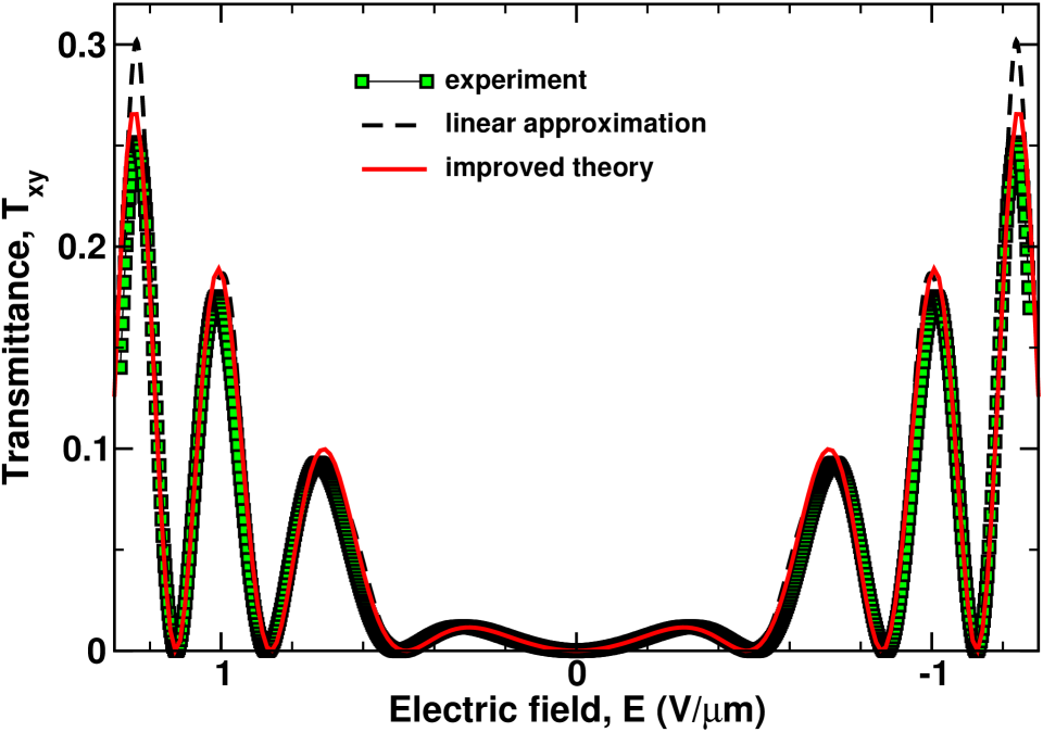
Figure 3: (Color online) Transmittance of light passing through crossed polarizers, $T_{xy}$, as a function of the applied electric field at the wavelength $\lambda=650$ nm for the DHFLC cell of thickness $D=130$ $\mu$m filled with the FLC mixture FLC-576A Kiselev et al. (2011). Parameters of the mixture are: $n_{\perp}=\sqrt{\epsilon_{\perp}}=1.5$ ($n_{\parallel}=\sqrt{\epsilon_{1}}=1.72$) is the ordinary (extraordinary) refractive index and $\theta=32$ deg is the tilt angle. The experimental points are marked by squares. The results obtained using the linear approximation are shown as dashed line Dashed and solid lines represent the theoretical curves computed using the linear approximation Kiselev et al. (2011) and the improved method of averaging with $P_{s}/\chi_{E}\approx 3.4$ V/$\mu$m, respectively.

Typically, in experiments dealing with the electro-optic response of DHFLC cells, the transmittance of normally incident light passing through crossed polarizers is measured as a function of the applied electric field. For normal incidence, the transmission and reflection matrices can be easily obtained from the results given in Appendix B by substituting Eq. (121) into Eqs. (107)- (108). When the incident wave is linearly polarized along the $x$ axis (the helix axis), the transmittance coefficient

$$T_{xy}=|t_{xy}|^{2}=\frac{|t_{+}-t_{-}|^{2}}{4}\,\sin^{2}(2\psi_{\mathrm{d}}),\quad\sin^{2}(2\psi_{\mathrm{d}})=\frac{\alpha_{E}^{2}}{\alpha_{E}^{2}+(\Delta\epsilon/\gamma_{xy})^{2}}\,,$$ (64)

$$t_{\pm}=\frac{1-\rho_{\pm}^{2}}{1-\rho_{\pm}^{2}\exp(2in_{\pm}h)}\exp(in_{\pm}h),\quad\rho_{\pm}=\frac{n_{\pm}/\mu-n_{\mathrm{m}}/\mu_{\mathrm{m}}}{n_{\pm}/\mu+n_{\mathrm{m}}/\mu_{\mathrm{m}}}.$$ (65)

where $h=k_{\mathrm{vac}}D$ is the thickness parameter, describes the intensity of the light passing through crossed polarizers. Note that, under certain conditions such as $|\rho_{\pm}|\ll 1$, $t_{\pm}\approx\exp(in_{\pm}h)$ and the transmittance (64) can be approximated by simpler formula

$$T_{xy}\approx\sin^{2}(\delta/2)\,\sin^{2}(2\psi_{\mathrm{d}}),$$ (66)

where $\delta=\Delta n_{\mathrm{eff}}\,h=(n_{+}-n_{-})h$ is the difference in optical path of the ordinary and extraordinary waves known as the phase retardation.

In Ref. Kiselev et al. (2011), the relation (64) was used to fit the experimental data using the theory based on the linear approximation for the helix distortions (see Eq. (43)). These results are reproduced in Figure 3 along with the theoretical curve computed using the modified averaging technique. From Fig. 3, it is seen that, in the range of relatively high voltages, the averaging method described in Appendix C improves agreement between the theory and the experiment, whereas, at small voltages, the difference between the fitting curves is negligibly small.

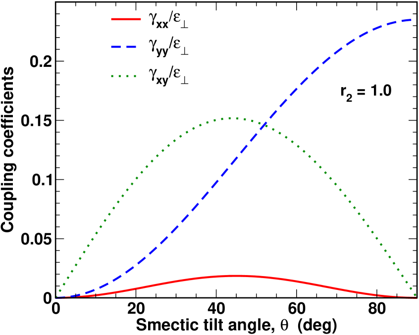
(a) $r_{2}=1.0$

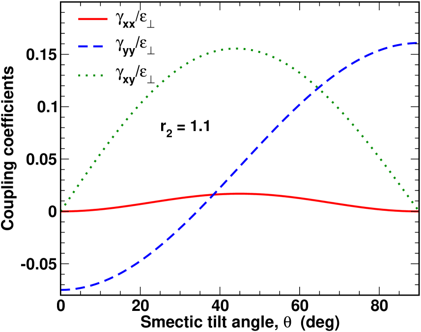
(b) $r_{2}=1.1$

Figure 4: (Color online) Coupling coefficients as a function of the smectic tilt angle $\theta$ at $r_{1}=(1.72/1.5)^{2}\approx 1.32$ for (a) a uniaxially anisotropic FLC with $r_{2}=1$ and (b) a biaxially anisotropic FLC with $r_{2}=1.1$.

III.3 Effects of smectic tilt angle

Given the anisotropy and biaxiality ratios, $r_{1}$ and $r_{2}$, the zero-field dielectric constants  (55) and the coupling coefficients (56) are determined by the smectic tilt angle, $\theta$. Figure 4 shows how the coupling coefficients depend on $\theta$ for both uniaxially and biaxially anisotropic FLCs.

As it can be seen in Fig. 4a, in the case of conventional FLCs with $r_{2}=1$, all the coefficients are positive and the difference of the coupling constants $\gamma_{xx}-\gamma_{yy}$ that define the electrically induced part of $\Delta\epsilon$ (see Eq. (62)) is negative at $0<\theta<\pi/2$.

From Eqs. (59) and (60), it follows that, at $r_{2}=1$, the principal values of dielectric constants $\epsilon_{z}$ and $\epsilon_{-}$ are decreasing functions of the electric field parameter $\alpha_{E}$ so that anisotropy of the effective dielectric tensor (54) is weakly biaxial. In addition, for non-negative $\alpha_{E}$ and $\gamma_{xx}-\gamma_{yy}<0$, the azimuthal angle of in-plane optical axis, $\psi_{\mathrm{d}}$, given in Eq. (63) increases with $\alpha_{E}$ from zero to $\pi/2$.

Figure 4b demonstrates that this is no longer the case for biaxial FLCs. It is seen that, at $r_{2}=1.1$, the coupling coefficient $\gamma_{yy}$ and the difference $\gamma_{xx}-\gamma_{yy}$ both change in sign when the tilt angle $\theta$ is sufficiently small. At such angles, the dielectric constant $\epsilon_{z}$ increases with $\alpha_{E}$ and the electric field induced anisotropy of DHFLC cell becomes strongly biaxial. When $\gamma_{xx}-\gamma_{yy}$ and $\alpha_{E}$ are positive, electric field dependence of the azimuthal angle $\psi_{\mathrm{d}}$ is non-monotonic and the angle decays to zero in the range of high voltages where $\psi_{\mathrm{d}}\propto\alpha_{E}^{-1}$.

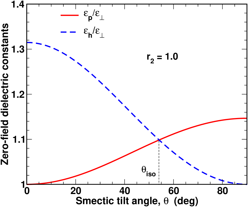
(a) $r_{2}=1.0$

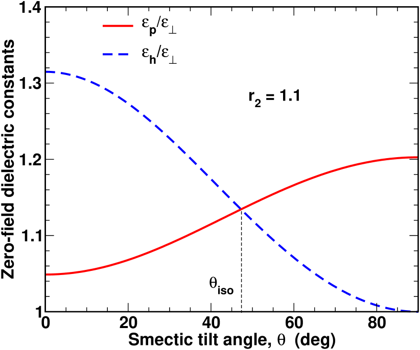
(b) $r_{2}=1.1$

Figure 5: (Color online) Zero-field dielectric constants as a function of the smectic tilt angle $\theta$ at $r_{1}=(1.72/1.5)^{2}\approx 1.32$ for (a) a uniaxially anisotropic FLC with $r_{2}=1$ and (b) a biaxially anisotropic FLC with $r_{2}=1.1$.

III.4 Zero-field isotropy and electro-optic response near exceptional point

At $E=0$, the zero-field anisotropy is uniaxial and is described by the dielectric constants, $\epsilon_{h}$ and $\epsilon_{p}$, given in Eq. (55). In Fig. 5, these constants are plotted against the tilt angle. It is shown that, at small tilt angles, the anisotropy $\epsilon_{h}-\epsilon_{p}$ is positive. It decreases with $\theta$ and the zero-field state becomes isotropic when, at certain critical angle $\theta=\theta_{\mathrm{iso}}$, the condition of zero-field isotropy

$$\epsilon_{p}=\epsilon_{z}$$ (67)

is fulfilled and $\Delta\epsilon_{0}=0$. So, the angle $\theta_{\mathrm{iso}}$ can be referred to as the isotropization angle. In what follows we discuss peculiarities of the electro-optic response in the vicinity of the isotropization point where $\Delta\epsilon$ is proportional to $E^{2}$ (see Eq. (62)) and the Kerr-like regime breaks down.

Mathematically, the isotropization point represents a square root branch-point singularity of the eigenvalues (60) of the dielectric tensor which is known as the exceptional point Kato (1995); Heiss and Sanino (1990); Heiss (2000). In the electric field dependence of the in-plane dielectric constants, $\epsilon_{+}$ and $\epsilon_{-}$, this singularity reveals itself as a cusp where the derivatives of $\epsilon_{\pm}$ with respect to $\alpha_{E}$ are discontinuous. More precisely, we have

$$\frac{\partial\epsilon_{+}}{\partial\alpha_{E}}\biggl{\lvert}_{\alpha_{E}=0\pm 0}=-\frac{\partial\epsilon_{-}}{\partial\alpha_{E}}\biggl{\lvert}_{\alpha_{E}=0\pm 0}=\pm|\gamma_{xy}|.$$ (68)

As is illustrated in Fig. 6a, the cusp is related to the effect of reconnection of different branches representing solutions of an algebraic equation.

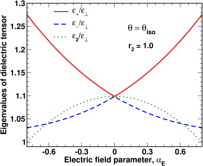
(a) $\theta=\theta_{\mathrm{iso}}\approx 54.11$ deg

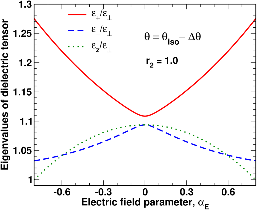
(b) $\Delta\theta=2$ deg

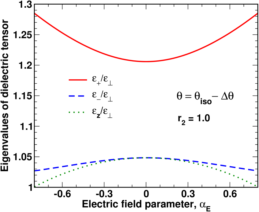
(c) $\Delta\theta=20$ deg

Figure 6: (Color online) Principal values of the effective dielectric tensor as a function of the electric field parameter at $r_{1}\approx 1.32$ and $r_{2}=1$ for different values of the smectic tilt angles.

Since the azimuthal angle $\psi_{\mathrm{d}}$ is undetermined at $\theta=\theta_{\mathrm{iso}}$

$$(\Delta\epsilon+i\gamma_{xy}\alpha_{E})\Bigl{\lvert}_{\alpha_{E}=0}=0\Longrightarrow\psi_{d}-?$$ (69)

the isotropization point also represents a phase singularity. The electric field dependence of $\psi_{\mathrm{d}}$ is thus discontinuous and the relation

$$\psi_{d}\Bigl{\lvert}_{\alpha_{E}=0+0}-\psi_{d}\Bigl{\lvert}_{\alpha_{E}=0-0}=\mathop{\rm sign}\nolimits(\gamma_{xy})\,\frac{\pi}{2}$$ (70)

describes its jumplike behaviour at $E=0$. This behaviour is demonstrated in Fig. 7.

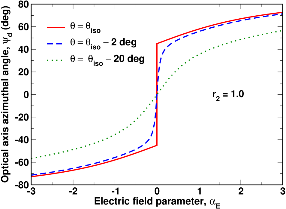
(a) $r_{2}=1.0$

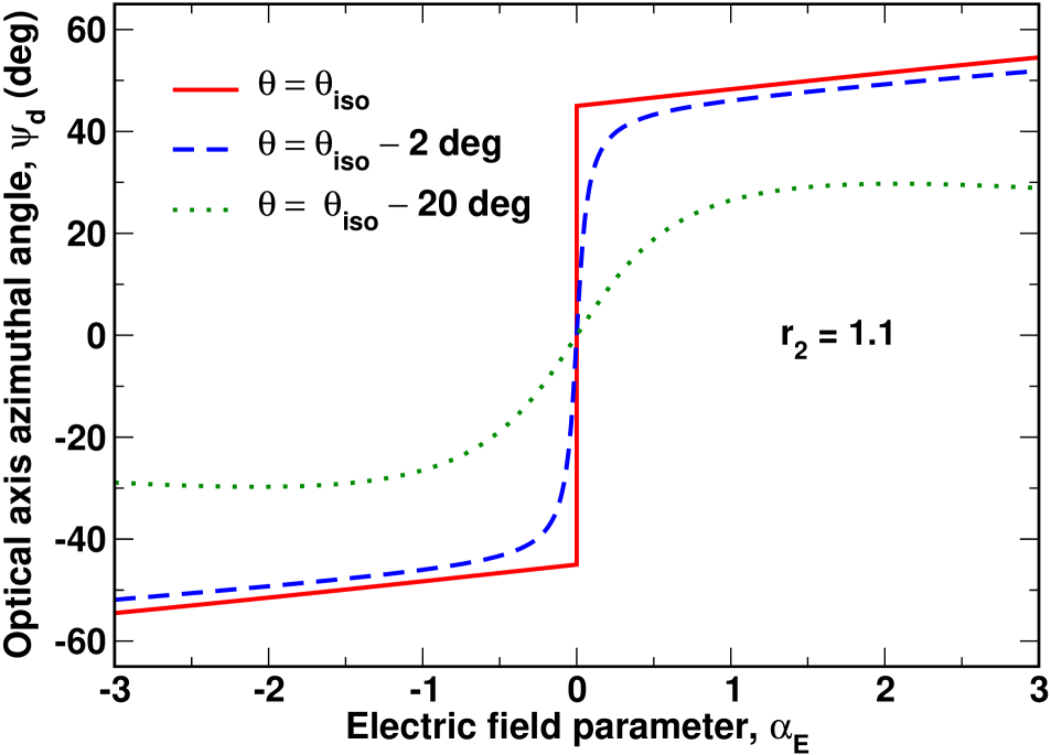
(b) $r_{2}=1.1$

Figure 7: (Color online) Principal axis azimuthal angle versus the electric field parameter at $r_{1}\approx 1.32$ for (a) a uniaxially anisotropic FLC with $r_{2}=1$ and (b) a biaxially anisotropic FLC with $r_{2}=1.1$.

We can now use Eq. (55) and write down the condition of zero-field isotropy (67) in the following explicit form:

$$r_{2}\sqrt{u}-\sqrt{r_{2}}=(u_{1}-u+1)\left(\frac{r_{2}-1}{\sqrt{u}+\sqrt{r_{2}}}+u^{-1/2}\right).$$ (71)

The case of a uniaxially anisotropic FLC with $r_{2}=1$ can be treated analytically. In this case, it is not difficult to check that $r_{1}=1$ gives the special solution of Eq. (71) that does not depend on the tilt angle and corresponds to an isotropic material with $r_{1}=r_{2}=1$. Another solution is given by the relation

$$\sin^{2}\theta_{\mathrm{iso}}=\frac{1}{2}+\frac{\sqrt{9+8u_{1}}-3}{8u_{1}}$$ (72)

linking the isotropization angle $\theta_{\mathrm{iso}}$ and the anisotropy parameter, $u_{1}=r_{1}-1$. In Fig. 8, this solution is represented by the solid line curve. The isotropization angle is shown to be a slowly decreasing function of the anisotropy ratio $r_{1}$. From Eq. (72), it starts from the maximal value of $\theta_{\mathrm{iso}}$ is $\pi/3$ and decays approaching $\pi/4$.

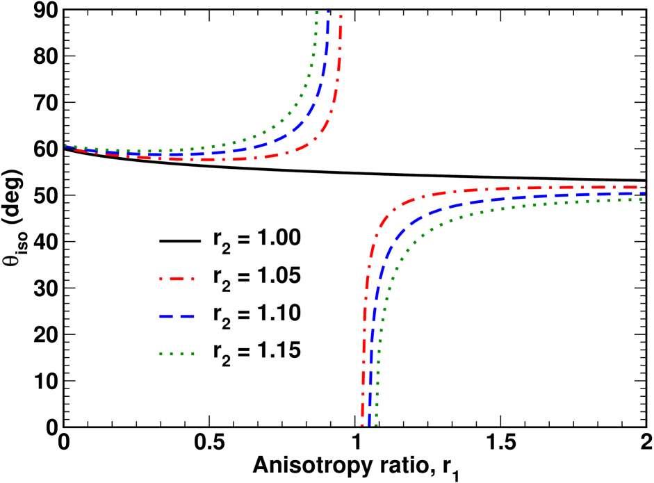
(a) $r_{2}\geq 1$

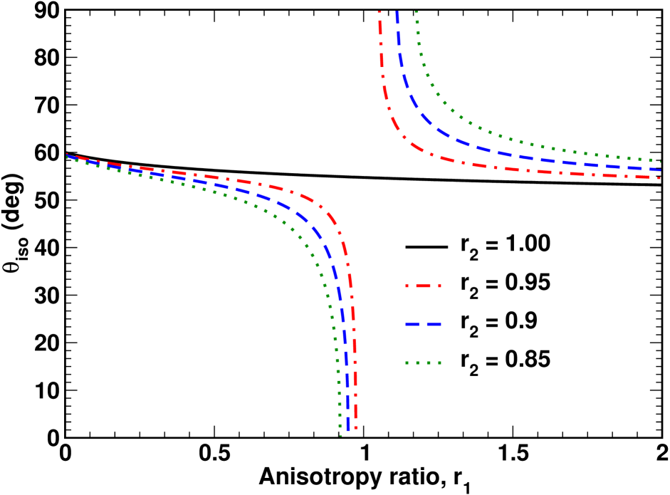
(b) $r_{2}\leq 1$

Figure 8: (Color online) Isotropization tilt angle versus the anisotropy ratio $r_{1}=\epsilon_{1}/\epsilon_{\perp}$ at different values of the biaxiality ratio $r_{2}=\epsilon_{2}/\epsilon_{\perp}$.

When the biaxiality ratio $r_{2}$ differs from unity, the solution of the isotropy condition (71) can only be written in the parametrized form as follows

$$\begin{cases}\sin^{2}\theta_{\mathrm{iso}}=(u-1)(R_{1}(u)-1)^{-1},\\ r_{1}=R_{1}(u),\end{cases}$$ (73)

where

$$R_{1}(u)/\sqrt{u}=\sqrt{u}+(\sqrt{u}+\sqrt{r_{2}})\frac{\sqrt{r_{2}u}-1}{\sqrt{r_{2}u}+1}.$$ (74)

The $\theta_{\mathrm{iso}}$ versus $r_{1}$ curves computed from the representation (73) are shown in Fig. 8. It can be seen that, by contrast to the case of uniaxial anisotropy [$r_{2}=1$], for biaxial FLCs with $r_{2}\neq 1$, each curve has two branches separated by a gap. The isotropization angle vanishes, $\theta_{\mathrm{iso}}=0$, at one of the endpoints of the gap, $r_{1}=\sqrt{r_{2}}$, whereas the angle $\theta_{\mathrm{iso}}$ equals $\pi/2$ at the other endpoint. Thus, dependence of the isotropization angle on the anisotropy ratio $r_{1}$ being smooth and continuous for uniaxially anisotropic FLCs is found to be splitted into two branches when the FLC anisotropy is biaxial. From Fig. 8, one of the branches with $u_{1}u_{2}>0$ is associated with the endpoint at $r_{1}=\sqrt{r_{2}}$ and lies below of the solid line curve representing conventional FLCs. For this branch, the angle $\theta_{\mathrm{iso}}$ decreases with the biaxiality ratio reaching zero at $r_{2}=r_{1}^{2}$.

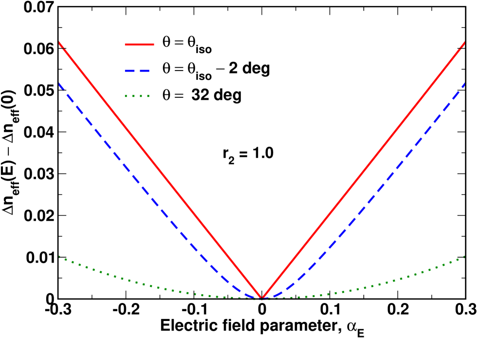
Figure 9: (Color online) Electrically controlled birefringence, $\Delta n_{\mathrm{eff}}(E)-\Delta n_{\mathrm{eff}}(0)$ [$\Delta n_{\mathrm{eff}}=n_{+}-n_{-}$], versus the electric field parameter at $r_{1}=1.32$ and $r_{2}=1$.

We conclude this section with the remark on the electro-optic response of DHFLC cells in the vicinity of the isotropization point. One of the important factors governing the electric field dependence of the transmittance (64) is the phase retardation $\delta$ (see Eq. (66)) proportional the effective birefringence $\Delta n_{\mathrm{eff}}=n_{+}-n_{-}$. The electrically dependent part of this birefringence is plotted as a function of the electric field parameter in Fig. 9. It shown that, at $\theta=\theta_{\mathrm{iso}}$, the Kerr-like regime breaks down and the birefringence is dominated by the terms linearly dependent on the electric field. Such a Pockels-like behaviour manifests itself in the perfectly harmonic dependence of the transmittance, $T_{xy}$, on the electric field parameter depicted in Fig. 10a.

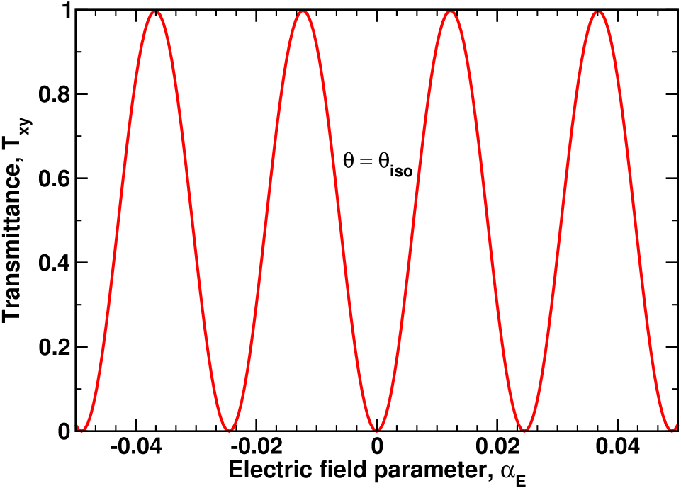
(a) $\theta=\theta_{\mathrm{iso}}\approx 54.11$ deg

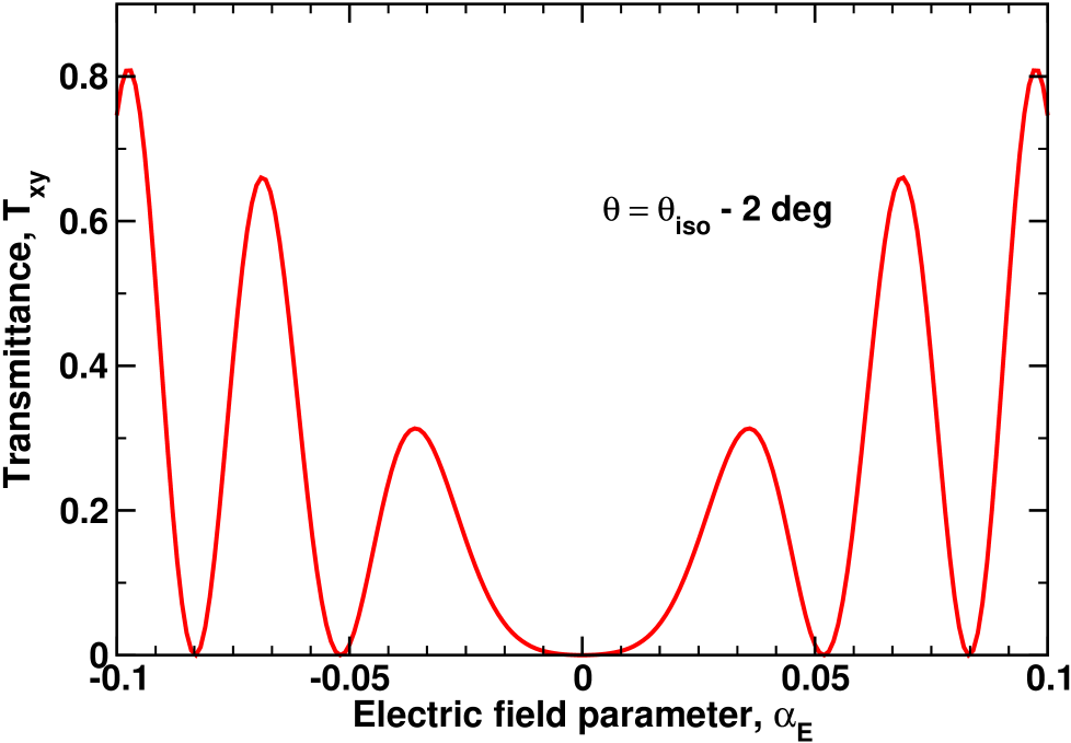
(b) $\Delta\theta=2$ deg

Figure 10: (Color online) Transmittance of light passing through crossed polarizers, $T_{xy}$, as a function of the electric field parameter at (a) $\theta=\theta_{\mathrm{iso}}\approx 54.11$ deg and (b) $\theta=52.11$ deg. Parameters are listed in the caption of Fig. 3.

Figure 10b illustrates the effect of small deviations from the isotropization angle. Though the curve presented in Fig. 10b and the ones for FLC-576A (see Fig. 3) are quite similar in shape, it is clear that sensitivity to the electric field and the magnitude of transmission peaks are both considerably enhanced near the isotropization point. Such behaviour comes as no surprise and derives from the above discussed fact that this point plays the role of a singularity (an exceptional point) (see Eqs. (68)–(70)).

IV Polarization-resolved angular patterns

We can now combine the general relations deduced in Sec. II (and in Appendix B) using the transfer matrix method with the results of Sec. III to study the polarization-resolved angular (conoscopic) patterns describing the polarization structure behind the conoscopic images of short-pitch DHFLC cells that are characterized by the effective dielectric tensor (49). This polarization structure is represented by a two-dimensional (2D) distribution of polarization ellipses and results from the interference of eigenmodes excited in the DHFLC cells by the plane waves with varying direction of incidence. Geometrically, the important elements of the 2D Stokes parameter fields are the polarization singularities such as $C$ points (the points where the light wave is circular polarized) and $L$ lines (the curves along which the polarization is linear). In this section the focus of our attention will be on the singularity structure of the polarization-resolved angular patterns emerging after the DHFLC cells. Our starting point is the computational method used to evaluate the patterns as the polarization ellipse fields.

IV.1 Computational procedure

We shall use the electric field vector amplitudes of incident, reflected and transmitted waves conveniently rewritten in the circular basis

$$\mathbf{E}_{\alpha}^{(c)}=\begin{pmatrix}E_{+}^{(\alpha)}\\ E_{-}^{(\alpha)}\end{pmatrix}=\mathbf{C}\begin{pmatrix}E_{p}^{(\alpha)}\\ E_{s}^{(\alpha)}\end{pmatrix},\quad\mathbf{C}=\frac{1}{\sqrt{2}}\begin{pmatrix}1&-i\\ 1&i\end{pmatrix},\quad\alpha\in\{\mathrm{inc},\mathrm{trm},\mathrm{refl}\}.$$ (75)

and the incidence angles, $\theta_{\mathrm{inc}}$ and $\phi_{\mathrm{inc}}$, related to the lateral component of the wave vector (6) as follows

$$q_{p}=n_{\mathrm{m}}\sin\theta_{\mathrm{inc}},\quad\phi_{p}=\phi_{\mathrm{inc}},$$ (76)

where $\theta_{\mathrm{inc}}$ ($\phi_{\mathrm{inc}}$) is the polar (azimuthal) angle of incidence. Dependence of the polarization properties of the waves transmitted through the DHFLC cell on the incidence angles, $\theta_{\mathrm{inc}}$ and $\phi_{\mathrm{inc}}$, will be of our primary concern.

The transmission matrix describing conoscopic patterns on the transverse plane of projection is given by Kiselev (2007a); Kiselev et al. (2008)

$$\mathbf{T}_{\mathrm{con}}(\rho,\phi)=\exp(-i\phi\boldsymbol{\sigma}_{3})\,\mathbf{T}_{c}(\rho,\psi_{d}-\phi)\,\exp(i\phi\boldsymbol{\sigma}_{3})$$ (77)

$$\mathbf{T}_{c}(\rho,\psi_{d}-\phi)=\begin{pmatrix}t_{++}&t_{+-}\\ t_{-+}&t_{--}\end{pmatrix}=\mathbf{C}\,\mathbf{T}(q_{p},\psi_{d}-\phi)\,\mathbf{C}^{\dagger},$$ (78)

$$\rho=r\tan\theta_{\mathrm{inc}},\quad\phi=\phi_{\mathrm{inc}},\quad q_{p}/n_{\mathrm{m}}=\frac{\rho}{\sqrt{r^{2}+\rho^{2}}},$$ (79)

where $\rho$ and $\phi$ are the polar coordinates in the observation plane ($x=\rho\cos\phi$ and $y=\rho\sin\phi$ are the Cartesian coordinates) and $r$ is the aperture dependent scale factor.

The transmission matrix of DHFLC cells, $\mathbf{T}(q_{p},\psi_{d}-\phi)$, can be computed from general formulas given in Appendix B (see Eq. (108)). For this matrix, the parameters $\{\epsilon_{z},\epsilon_{\parallel},\epsilon_{\perp},\psi\}$ that enter the expression for the dielectric tensor of planar structures (96) should be replaced with the characteristics $\{\epsilon_{z},\epsilon_{+},\epsilon_{-},\psi_{d}-\phi\}$ of the effective dielectric tensor (54) given in Eqs. (58)– (63). In what follows the incident light is assumed to be linearly polarized

$$\mathbf{E}_{\mathrm{inc}}^{(c)}=E_{\mathrm{inc}}\exp(-i\phi_{p}^{(\mathrm{inc})}\boldsymbol{\sigma}_{3})\begin{pmatrix}1\\ 1\end{pmatrix},$$ (80)

where $\phi_{p}^{(\mathrm{inc})}$ is the polarization azimuth of the incident wave, and the state of polarization of the transmitted wave

$$\mathbf{E}_{\mathrm{trm}}^{(c)}=\begin{pmatrix}E_{+}^{(\mathrm{trm})}\\ E_{-}^{(\mathrm{trm})}\end{pmatrix}=\mathbf{T}_{\mathrm{con}}(\rho,\phi)\mathbf{E}_{\mathrm{inc}}^{(c)},$$ (81)

is defined by the polarization ellipse characteristics. The orientation of the polarization ellipse is specified by the azimuthal angle of polarization (polarization azimuth)

$$2\phi_{p}^{(\mathrm{trm})}=\arg S\equiv\chi_{s},\quad S=S_{1}+iS_{2}=2{[E_{+}^{(\mathrm{trm})}]}^{\ast}E_{-}^{(\mathrm{trm})},$$ (82)

where $S_{i}$ is the $i$th component of the Stokes vector, and its eccentricity is described by the signed ellipticity parameter

$$\epsilon_{\mathrm{ell}}^{(\mathrm{trm})}=\frac{|E_{+}^{(\mathrm{trm})}|-|E_{-}^{(\mathrm{trm})}|}{|E_{+}^{(\mathrm{trm})}|+|E_{-}^{(\mathrm{trm})}|}=\tan\{2^{-1}\arcsin(S_{3}/S_{0})\},\quad S_{3,\,0}=|E_{+}^{(\mathrm{trm})}|^{2}\mp|E_{-}^{(\mathrm{trm})}|^{2}$$ (83)

that will be referred to as the ellipticity. The ellipse is considered to be right handed (left handed) if its helicity is positive (negative), so that $\epsilon_{\mathrm{ell}}^{(\mathrm{trm})}>0$ ($\epsilon_{\mathrm{ell}}^{(\mathrm{trm})}<0$).

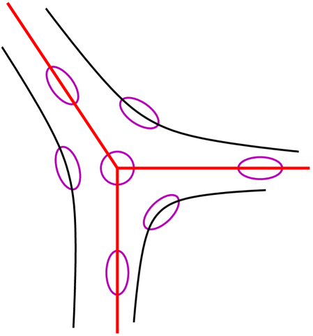
(a) Star: $I_{C}=-1/2$ and $N_{C}=3$

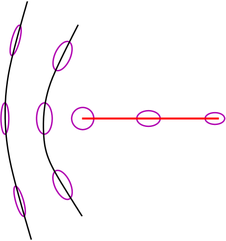
(b) Lemon: $I_{C}=+1/2$ and $N_{C}=1$

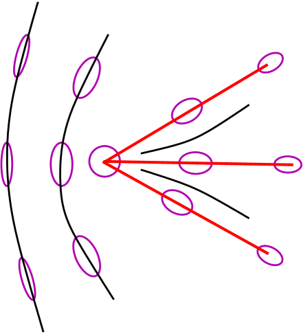
(c) Monstar: $I_{C}=+1/2$ and $N_{C}=3$

Figure 11: (Color online) Arrangement of the polarization ellipses around the $C$ points of three different types.

From Eq. (79), the incidence angles and the points in the observation plane are in one-to-one correspondence. So, computing the polarization azimuth, $\phi_{p}^{(\mathrm{trm})}$, the ellipticity, $\epsilon_{\mathrm{ell}}^{(\mathrm{trm})}$, at each point of the projection plane yields the 2D field of polarization ellipses which is called the polarization-resolved angular (conoscopic) pattern.

The point where $E_{\nu}^{(\mathrm{trm})}=0$ and thus the transmitted wave is circularly polarized with $\epsilon_{\mathrm{ell}}^{(\mathrm{trm})}=-\nu$ will be referred to as the C_ν point.

This is an example of the polarization singularity that can be viewed as the phase singularities of the complex scalar field $S=S_{1}+iS_{2}$ where the phase $\chi_{s}$ (see Eq. (82)) become indeterminate. Such singularities are characterized by the winding number which is the signed number of rotations of the two-component field $(S_{1},S_{2})$ around the circuit surrounding the singularity Mermin (1979). The winding number also known as the signed strength of the dislocation is generically $\pm 1$.

Since the polarization azimuth (82) is defined modulo $\pi$ and $2\phi_{p}=\arg S$, the dislocation strength is twice the index of the corresponding $C_{\nu}$ point, $I_{C}$. For generic $C$ points, $I_{C}=\pm 1/2$ and the topological index can be computed as the closed-loop contour integral of the phase $\chi_{s}$ modulo $4\pi$

$$I_{C}=\frac{1}{4\pi}\oint_{L}\mathrm{d}\chi_{s},$$ (84)

where $L$ is the closed path around the singularity.

In addition to the handedness and the index, the $C$ points are classified according to the number of streamlines, which are polarization lines whose tangent gives the polarization azimuth, terminating on the singularity. This is the so-called line classification that was initially studied in the context of umbilic points Berry and Hannay (1977). Mathematically, the straight streamlines that terminate on the singularity are of particular importance as they play the role of separatrices, separating regions of streamlines with differently signed curvature. As is illustrated in Fig. 11, for generic $C$ points, the number of the straight lines, $N_{C}$, may either be 1 or 3. This number is $3$ provided the index equals $-1/2$, $I_{C}=-1/2$, and such $C$ points are called stars. At $I_{C}=1/2$, there are two characteristic patterns of polarization ellipses around a $C$ point: (a) lemon with $N_{C}=1$ and (b) monstar with $N_{C}=3$ Nye (1983). Different quantitative criteria to distinguish between the $C$ points of the lemon and the monstar types were deduced in Refs. Dennis (2002); Kiselev (2007b). From these criteria it can be inferred that a lemon becomes a monstar as it approaches a star and $C$ point annihilation occurs only between stars and monstars Dennis (2002, 2008).

The case of linearly polarized wave with $\epsilon_{\mathrm{ell}}^{(\mathrm{trm})}=0$ provides another example of the polarization singularity where the handedness is undefined. The curves along which the polarization is linear are called the L lines.

From Eq. (82) the $C$ points are nodal points of the scalar complex function $S$ which can be found as intersection points of the Stokes parameter nodal lines $S_{1}=0$ and $S_{2}=0$. Similarly, equation (83) implies that nodes of the Stokes parameter field $S_{3}$ provide the $L$ lines where $S_{3}=0$ and $\epsilon_{\mathrm{ell}}^{(\mathrm{trm})}=0$.

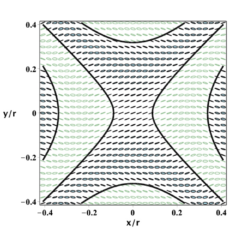
(a) $\alpha_{E}=0$ and $\psi_{d}-\phi_{p}^{(\mathrm{inc})}=20$ deg

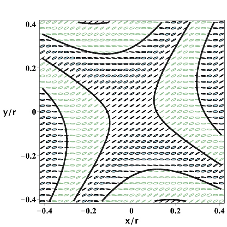
(b) $\alpha_{E}=0.3$ and $\psi_{d}-\phi_{p}^{(\mathrm{inc})}=20$ deg

Figure 12: (Color online) Polarization-resolved conoscopic patterns computed as polarization ellipse fields in the observation plane for the DHFLC cell filled with the FLC mixture FLC-576A (see Ref. Kiselev et al. (2011) and the caption of Fig. 3). Two cases are shown: (a) $\alpha_{E}=0$ ($n_{+}\approx 1.65$, $n_{-}=n_{z}\approx 1.532$ and $\psi_{d}=0$) and (b) $\alpha_{E}=0.3$ ($n_{+}\approx 1.66$, $n_{-}\approx 1.529$ $n_{z}\approx 1.527$ and $\psi_{d}=13$ deg). In both cases, the angle between the in-plane optical axis and the polarization plane of the incident light is fixed at $\psi_{d}-\phi_{p}^{(\mathrm{inc})}=20$ deg. $L$ lines are represented by thick black solid lines. Left-handed and right-handed polarization is, respectively, indicated by solid and open ellipses.

IV.2 Results

Now we present the theoretical results for the polarization-resolved patterns of the DHFLC cells. These patterns are computed for the cell of thickness $D=130$ $\mu$m filled with the FLC mixture FLC-576A which was studied in Ref. Kiselev et al. (2011) and described at the end of Sec. III.2.

Our first remark is that the angular dependence of the elements of the transmission matrix (78) is determined by the angle difference $\tilde{\phi}=\phi-\psi_{d}$ which is the angle between the in-plane optical axis $\hat{\mathbf{d}}_{+}$ (see Eq. (63)) and the lateral wave vector $\mathbf{q}_{p}$ (see Eq. (6)). Then the vector amplitudes

$$\tilde{\mathbf{E}}_{\mathrm{inc}}^{(c)}=\exp(i\psi_{d}\boldsymbol{\sigma}_{3})\mathbf{E}_{\mathrm{inc}}^{(c)}=E_{\mathrm{inc}}\exp(-i\tilde{\phi}_{p}^{(\mathrm{inc})}\boldsymbol{\sigma}_{3})\begin{pmatrix}1\\ 1\end{pmatrix},$$ (85a)

$$\tilde{\mathbf{E}}_{\mathrm{trm}}^{(c)}=\exp(i\psi_{d}\boldsymbol{\sigma}_{3})\mathbf{E}_{\mathrm{trm}}^{(c)}=E_{\mathrm{trm}}\exp(-i\tilde{\phi}_{p}^{(\mathrm{trm})}\boldsymbol{\sigma}_{3})\begin{pmatrix}1+\epsilon_{\mathrm{ell}}^{(\mathrm{trm})}\\ 1-\epsilon_{\mathrm{ell}}^{(\mathrm{trm})}\end{pmatrix},$$ (85b)

$$\tilde{\phi}_{p}^{(\mathrm{inc},\,\mathrm{trm})}=\phi_{p}^{(\mathrm{inc},\,\mathrm{trm})}-\psi_{d},$$ (85c)

where $\tilde{\phi}_{p}^{(\mathrm{inc})}$ is the angle between the optical axis $\hat{\mathbf{d}}_{+}$ and the polarization plane of the linearly polarized incident wave (see Eq. (80)), describing the incident and transmitted waves with polarization ellipses rotated by the angle $\psi_{p}$ are related by the transformed transmission matrix

$$\tilde{\mathbf{T}}_{\mathrm{con}}(\tilde{\phi})=\exp(i\psi_{d}\boldsymbol{\sigma}_{3})\,\mathbf{T}_{\mathrm{con}}\,\exp(-i\psi_{d}\boldsymbol{\sigma}_{3})=$$

$$\exp[-i\tilde{\phi}\boldsymbol{\sigma}_{3}]\,\mathbf{T}_{c}(\rho,-\tilde{\phi})\,\exp[i\tilde{\phi}\boldsymbol{\sigma}_{3}].$$ (86)

From relation (IV.2) it follows that, given the angle $\tilde{\phi}_{p}^{(\mathrm{inc})}$, the sole effect of changing the azimuthal angle of the optical axis: $\psi_{d}\to\psi_{d}+\Delta\psi$ is the rotation of the polarization ellipse field by the angle $\Delta\psi$. In DHFLC cells, this effect manifests itself as the electric field induced rotation and can be clearly seen in Fig. 12 that shows the patterns emerging after the DHFLC cell calculated at $\tilde{\phi}_{p}^{(\mathrm{inc})}=-20$ deg for two values of the electric filed parameter: $\alpha_{E}=0$ (see Fig. 12a) and $\alpha_{E}=0.3$ (see Fig. 12b).

Figure 12 also illustrates the case of angular patterns that do not contain $C$ points. The geometry of such patterns is completely characterized by the $L$ lines. Interestingly, at $|\tilde{\phi}_{p}^{(\mathrm{inc})}|>5$ deg, it turned out that the $S_{3}$ nodal lines can be evaluated using the simplified equation

$$\sin\delta=0,\quad\delta=(q_{e}-q_{o})h,$$ (87)

where $\delta$ is the phase retardation expressed in terms of the eigenvalues of the matrix (9) for uniformly anisotropic planar layers (see Eqs. (114) and (117)), that thus gives a sufficiently accurate approximation for $L$ lines.

The angle $\tilde{\phi}_{p}^{(\mathrm{inc})}$ can be regarded as the governing parameter whose magnitude determines the formation of $C$ points. Given the aperture, the latter occurs only if the magnitude of $\tilde{\phi}_{p}^{(\mathrm{inc})}$ exceeds its critical value.

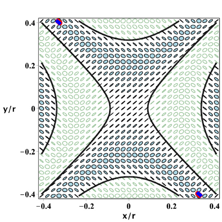
(a) $\alpha_{E}=0$ and $\psi_{d}-\phi_{p}^{(\mathrm{inc})}=39.5$ deg

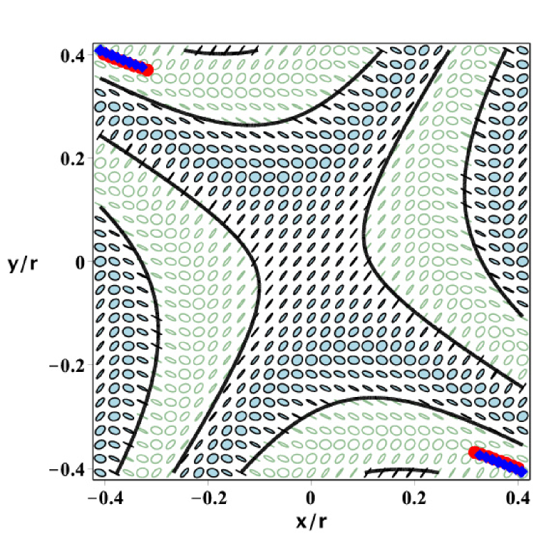
(b) $\alpha_{E}=0.3$ and $\psi_{d}-\phi_{p}^{(\mathrm{inc})}=39.5$ deg

Figure 13: (Color online) Polarization-resolved conoscopic patterns computed as polarization ellipse fields in the observation plane for the DHFLC cell at $\psi_{d}-\phi_{p}^{(\mathrm{inc})}=39.5$ deg (see the caption of Fig. 12). Two cases are shown: (a) $\alpha_{E}=0$ and (b) $\alpha_{E}=0.3$. $C$ points are indicated by red circles (stars with $I_{C}=-1/2$) and blue diamonds (monstars with $I_{C}=1/2$).

The case where the angle $\tilde{\phi}_{p}^{(\mathrm{inc})}$ is close to the critical value is illustrated in Fig. 13a. It can be seen that, at $\tilde{\phi}_{p}^{(\mathrm{inc})}=-39.5$ deg, the singularity structure of the polarization ellipse fields becomes complicated and is characterized by the presence of symmetrically arranged star-monstar pairs of $C$ points. In addition to the above discussed electric-field-induced rotation, the electric field is shown to facilitate the formation of $C$ points. Clearly, the field induced biaxial anisotropy is responsible for this effect.

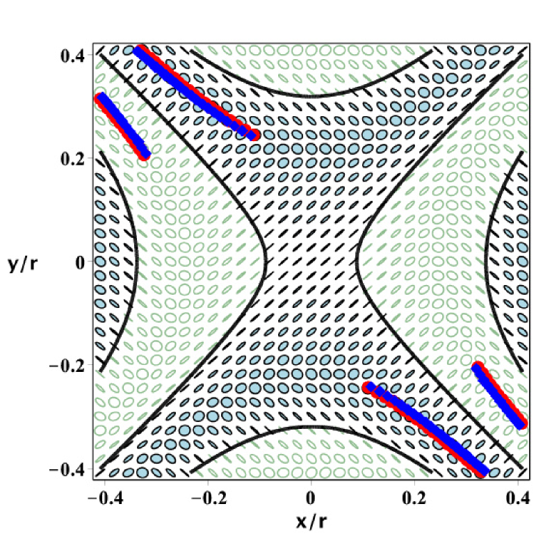
(a) $\alpha_{E}=0$ and $\psi_{d}-\phi_{p}^{(\mathrm{inc})}=41$ deg

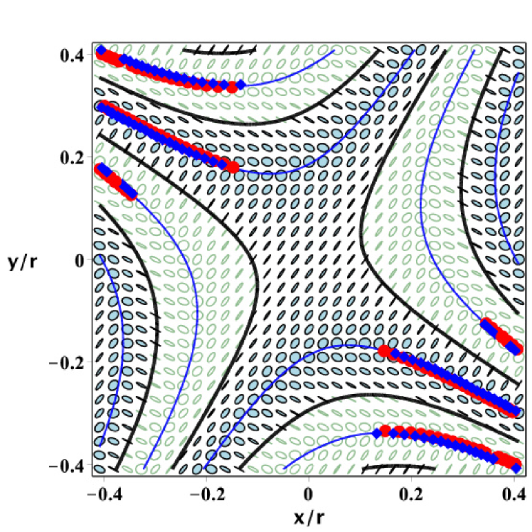
(b) $\alpha_{E}=0.3$ and $\psi_{d}-\phi_{p}^{(\mathrm{inc})}=41$ deg

Figure 14: (Color online) Polarization-resolved conoscopic patterns computed as polarization ellipse fields in the observation plane for the DHFLC cell at $\psi_{d}-\phi_{p}^{(\mathrm{inc})}=41$ deg (see the caption of Fig. 12). Two cases are shown: (a) $\alpha_{E}=0$ and (b) $\alpha_{E}=0.3$. $C$ points with $I_{C}=-1/2$ and $I_{C}=+1/2$ are indicated by red circles (stars) and blue diamonds (monstars), respectively. Blue thin solid lines represent the approximate $S_{2}$ nodal lines computed by solving equation (88).

In Fig. 14, we show how the singularity structure of the polarization resolved patterns develops when the angle $\tilde{\phi}_{p}^{(\mathrm{inc})}$ further increases. This structure can be described as symmetrically arranged chains of star-monstar pairs of $C$ points. As is indicated in Fig. 14b, these tightly packed chains of $C$ points are generally located in the vicinity of the lines

$$\cos\delta=0$$ (88)

that give a high accuracy approximation for the $S_{2}$ nodal lines where $S_{2}=0$ and, similar to Eq. (87), are determined by the phase retardation $\delta=(q_{e}-q_{o})h$. Note that, since $S_{2}-iS_{3}=2{[E_{s}^{(\mathrm{trm})}]}^{\ast}E_{p}^{(\mathrm{trm})}$, applicability of approximate formulas (87) and (88) implies that the phase difference between the components of the transmitted waves, $E_{p}^{(\mathrm{trm})}$ and $E_{s}^{(\mathrm{trm})}$, is close to the phase retardation: $\arg\{{[E_{s}^{(\mathrm{trm})}]}^{\ast}E_{p}^{(\mathrm{trm})}\}\approx\delta$. In Sec. III.2, a similar approximation has been used to derive the expression for the transmittance given by Eq. (66).

As it was mentioned in the previous section, the loci of $C$ points on the projection plane are determined by intersections of the $S_{2}$ and $S_{1}$ nodal lines. In our case, the star-monstar pairs are produced as a result of small-scale oscillations of the nodal line around the smooth curve described by Eq. (88). Experimentally, it is a challenging task to resolve accurately the chains of $C$ points resulting from such ripplelike oscillations in polarimetry measurements.

The 2D polarization-resolved patterns are centrally symmetric being invariant under inversion through the origin: $(x,y)\to(-x,-y)$. The reason is that optical properties of planar anisotropic structures are unchanged under a 180-degree rotation about the normal to the cell (the $z$ axis). More specifically, we have the central symmetry relation

$$\tilde{\mathbf{T}}_{\mathrm{con}}(\tilde{\phi})=\tilde{\mathbf{T}}_{\mathrm{con}}(\tilde{\phi}+\pi)$$ (89)

which is an immediate consequence of the fact that the matrix $\mathbf{M}$ given in Eqs. (99) and (100) remains intact when the azimuthal angle of the in-plane optic axis is changed by $\pi$.

Another symmetry relation

$$\tilde{\mathbf{T}}_{\mathrm{con}}(-\tilde{\phi})=\boldsymbol{\sigma}_{1}\tilde{\mathbf{T}}_{\mathrm{con}}(\tilde{\phi})\boldsymbol{\sigma}_{1}$$ (90)

describes the transformation of the transmission matrix (IV.2) under reflection in the mirror symmetry axis directed along $\hat{\mathbf{d}}_{+}$: $\tilde{\phi}\to-\tilde{\phi}$. This relation immediately follows from Eq. (113) deduced in Appendix B. By using formula (90), it is not difficult to show that the polarization ellipse field $\{\tilde{\phi}_{p}^{(\mathrm{trm})}(\rho,\tilde{\phi}),\epsilon_{\mathrm{ell}}^{(\mathrm{trm})}(\rho,\tilde{\phi})\}$ transforms into its mirror symmetric counterpart $\{-\tilde{\phi}_{p}^{(\mathrm{trm})}(\rho,-\tilde{\phi}),-\epsilon_{\mathrm{ell}}^{(\mathrm{trm})}(\rho,-\tilde{\phi})\}$ when the polarization azimuth $\tilde{\phi}_{p}^{(\mathrm{inc})}$ changes its sign: $\tilde{\phi}_{p}^{(\mathrm{inc})}\to-\tilde{\phi}_{p}^{(\mathrm{inc})}$.

V Discussion and conclusions

In this paper, we have performed transfer matrix analysis of polarization-resolved angular patterns emerging after electrically controlled short-pitch DHFLC cells. Our formulation of the transfer matrix method, which is a suitably modified version of the approach developed in Refs. Kiselev (2007a); Kiselev et al. (2008, 2011), involves the following steps: (a) derivation of the system of equations for the tangential components of the wave field in the $4\times 4$ matrix form (see Eq. (8)); (b) introducing the evolution operator (propagator) (10) and the scattering matrix (21); (c) defining the transfer matrix (25) through the propagator and, finally, (d) deducing formulas (II.2) that link the transfer and scattering matrices. Description of this method is augmented by discussion of a variety of unitarity and symmetry relations (see Sec. II.3 and Appendix B), with an emphasis on the special case of anisotropic planar structures representing homogenized DHFLC cells. Interestingly, the relations given in Eqs. (37), (110) and (113) are shown to be essentially independent of the assumption of lossless materials and thus can be used when the medium is absorbing.

In general, we found that, owing to its mathematical structure, the transfer matrix approach provides the framework particularly useful for in-depth analysis of symmetry related properties (recent examples of such analysis can be found, e.g., in Refs. Altman and Suchy (2011); Dmitriev (2013); Luque-Raigon et al. (2014)). Similarly, one of the important results of a rigorous analysis performed within such a framework in Ref. Kiselev et al. (2011) is the expression for the effective dielectric tensor (46) describing the electro-optical properties of uniform lying FLC helical structures with subwavelengh pitch.

In Sec. III we have extended theoretical considerations of Ref. Kiselev et al. (2011) to the case of biaxial FLCs and have applied an alternative technique of averaging over distorted helix to evaluate the dielectric tensor. This technique is presented in Appendix C and gets around the difficulties of the method that relies on the well-known first-order expression for a weakly distorted helix (43). The modified averaging procedure allows high-order corrections to the dielectric tensor to be accurately estimated and improves agreement between the theory and the experimental data in the high-field region (see Fig. 3).

The resulting electric field dependence of the effective dielectric tensor (54) is linear (quadratic) for non-diagonal (diagonal) elements with the coupling coefficients given by Eq. (56). These coupling coefficients along with the zero-field dielectric constants (55) determine how the applied electric field $E$ changes the principal values of the effective dielectric tensor (see Eqs. (59) and (60)) and the azimuthal angle of optical axis (63).

Generally, at $E=0$, the DHFLC cell is uniaxially anisotropic with the dielectric constants (55), $\epsilon_{p}$ and $\epsilon_{h}$, and the optical axis directed along the helix axis. Then there are two most important effects induced by the electric field: (a) producing biaxial anisotropy by changing the eigenvalues of the dielectric tensor; and (b) rotation of in-plane optical axes by the field dependent angle $\psi_{d}$ defined in Eq (63). At sufficiently low electric field $E$ and non-vanishing zero-field anisotropy, the Kerr-like regime takes place so that the principal values depend on the electric field quadratically whereas the optical axis angle $\psi_{d}$ is approximately proportional to $E$. This is the orientational Kerr effect previously studied in Refs. Kiselev et al. (2011); Pozhidaev et al. (2013, 2014) for different geometries.

Our results on dependence of the coupling coefficients and the zero-field dielectric constants on the smectic tilt angle $\theta$ described in Sec. III.3 indicate a number of differences between uniaxial and biaxial FLCs. What is more important, they show that the zero-field anisotropy may vanish at certain value of $\theta$ which might be called the isotropization angle: $\theta=\theta_{\mathrm{iso}}$ (see Fig. 5).

In Sec. III.4, the isotropization point determined by the condition of zero-field isotropy (67) is found to represent a singularity known as the exceptional point Kato (1995). For analytic continuation of the dielectric tensor (54) in the complex $\alpha_{E}$ plane, the exceptional points occur at the zeros of the square root in Eq. (60) where $[\Delta\epsilon]^{2}+[\gamma_{xy}\alpha_{E}]^{2}=0$. In general, there are two pairs of complex conjugate values of electric field parameter representing four exceptional (branch) points. When the difference $\epsilon_{h}-\epsilon_{p}$ vanishes, the two branch points coalesce on the real axis at the origin.

In the case of conventional uniaxial FLCs, the analytic solution of the condition of zero-field isotropy can be obtained in the closed form and is given by simple formula (72) where the isotropization angle, $\theta_{\mathrm{iso}}$, is found to be a decreasing function of the anisotropy parameter $u_{1}=(\epsilon_{1}-\epsilon_{\perp})/\epsilon_{\perp}=r_{1}-1$. For biaxial FLCs with $r_{2}=\epsilon_{2}/\epsilon_{\perp}\neq 1$, the solution can only be written in the parametrized form (73). As it can be seen in Fig. 8, the corresponding $\theta_{\mathrm{iso}}$-$r_{1}$ curves are splitted into two branches separated by the gap. These results significantly differ from the relation $\cos^{2}\theta_{\mathrm{iso}}=(1+u_{2}/u_{1})/3$ that can be easily obtained Abdulhalim (2012) for the dielectric tensor (41) averaged over the FLC helix: $\langle{\boldsymbol{\epsilon}}\rangle/\epsilon_{\perp}=[1+(u_{1}\sin^{2}\theta+u_{2})/2]\mathbf{I}_{3}+[u_{1}\cos^{2}\theta-(u_{1}\sin^{2}\theta+u_{2})/2]\hat{\mathbf{x}}\otimes\hat{\mathbf{x}}$. The difference stems from the fact that, in our approach, the effective dielectric tensor $\boldsymbol{\epsilon}_{\mathrm{eff}}$ is defined through the averaged differential propagation matrix $\langle{\mathbf{M}}\rangle$ and thus is not equal to the averaged dielectric tensor (41): $\boldsymbol{\epsilon}_{\mathrm{eff}}\neq\langle{\boldsymbol{\epsilon}}\rangle$

At the exceptional point, the Kerr-like regime breaks down and the electric field dependence of the birefringence becomes linear (see Fig. 9). This might be called the Pockels-like regime which is characterized by the harmonic electric field dependence of the transmittance of light passing through crossed polarizers (see Fig. 10a). The curve shown in Fig. 10b illustrates the electro-optical response of a DHFLC cell near the exceptional point. It is seen that sensitivity to the electric field and the magnitude of the transmittance at peaks are both considerably enhanced as compared to the case studied in Ref. Kiselev et al. (2011) (see also Fig. 3).

We now try to put these results in a more general physical context. In quantum physics, the exceptional points are known to produce a variety of interesting phenomena including level repulsion and crossing, bifurcation, chaos and quantum phase transitions Heiss and Sanino (1990); Heiss (2000); Song and Cao (2010); Lee et al. (2012). For optical wave fields, a recent example is unidirectional propagation (reflection) of light at the exceptional points in parity-time ($\mathcal{PT}$) symmetric periodic structures and metamaterials that has been the subject of intense studies Lin et al. (2011); Yin and Zhang (2013); Kang et al. (2014).

To the best of our knowledge, the role of exceptional points in optics of liquid crystal systems has yet to be recognized. The main problem with conventional uniaxial FLCs is that the isotropy condition (67) requires large values of the smectic tilt angle that are typically well above $50$ deg. Though there are no fundamental limitations preventing preparation of FLC mixtures with large tilt angles, this task still remains a challenge to deal with in the future. Biaxial FLCs, where the isotropization tilt angle can be sufficiently small when $\epsilon_{1}$ is close to $\sqrt{\epsilon_{2}}$, also present a promising alternative approach for future work.

In Sec. IV, in order to gain further insight into the electro-optical properties of the DHFLC cells, we have combined the transfer matrix approach and the results for the effective dielectric tensor to explore the polarization-resolved angular patterns which are the polarization ellipse fields representing the polarization structure of conoscopic images of DHFLC cells. In the observation plane, such 2D patterns encode information on how the polarization state of transmitted light is changed with the incidence angles and exhibit singularities of a different kind, the polarization singularities such as $L$ lines (lines of linear polarization) and $C$ points (points of circular polarization). Note that, similar to the above discussed exceptional point at which the angle $\psi_{d}$ becomes undetermined, $C$ points can be regarded as phase singularities (optical phase singularities are reviewed in Ref. Dennis et al. (2009)).

Since the differential propagation matrix of planar structures is invariant under rotation of in-plane optical axes by $\pi$, the patterns are centrally symmetric [see Figs. 12- 14]. It was shown that, at fixed the angle $\tilde{\phi}_{p}^{(\mathrm{inc})}=\psi_{d}-\phi_{p}^{(\mathrm{inc})}$ between the optical axis $\hat{\mathbf{d}}_{+}$ and the polarization plane of incident wave, the sole effect of the electric-field-induced rotation by the angle $\psi_{d}$ is rotation of the polarization ellipse field as a whole by the same angle.

The symmetry axis of the $S_{3}$ nodal lines ($L$ lines) is found to be directed along $\hat{\mathbf{d}}_{+}$. When the $\tilde{\phi}_{p}^{(\mathrm{inc})}$ is not too small, they can be approximated by solving Eq. (87) and thus are mainly determined by the phase retardation $\delta$. Similar remark applies to the $S_{2}$ lines and approximate formula (88).

It turned out that this is the angle $\tilde{\phi}_{p}^{(\mathrm{inc})}$ that plays the role of the parameter governing formation of $C$ points. When the magnitude of $\tilde{\phi}_{p}^{(\mathrm{inc})}$ exceeds its critical value which, in our case, is close to $39$ deg, $C$ points emerge as symmetrically arranged and densely packed chains of star-monstar pairs (see Figs. 13-14).

So, in DHFLC cells, rotation of polarization ellipse fields and formation of $C$ points are two most important effects describing electrically induced transformations of the polarization-resolved angular patterns. These predictions can be verified experimentally. This work is now in progress.

Appendix A Operator of evolution

We begin with the relation

$$\mathbf{U}(\tau,\tau_{0})=\mathbf{U}(\tau,\tau_{1})\cdot\mathbf{U}(\tau_{1},\tau_{0})$$ (91)

known as the composition law. This result derives from the fact that the operator $\mathbf{U}(\tau,\tau_{0})\cdot\mathbf{U}^{-1}(\tau_{1},\tau_{0})$ is the solution of the system (11a) that satisfies the initial condition (11b) with $\tau_{0}$ replaced by $\tau_{1}$.

From the composition law (91) it immediately follow that the inverse of the evolution operator is given by

$$\mathbf{U}^{-1}(\tau,\tau_{0})=\mathbf{U}(\tau_{0},\tau)$$ (92)

and can be found by solving the initial value problem

$$i\partial_{\tau}\mathbf{U}^{-1}(\tau,\tau_{0})=\mathbf{U}^{-1}(\tau,\tau_{0})\cdot\mathbf{M}(\tau),\quad\mathbf{U}^{-1}(\tau_{0},\tau_{0})=\mathbf{I}_{4}.$$ (93)

For non-absorbing media with symmetric dielectric tensor, the matrix $\mathbf{M}$ is real-valued, ${\mathbf{M}}^{\ast}=\mathbf{M}$, and meets the following symmetry identities Kiselev et al. (2008):

$${\mathbf{M}}^{\ast}=\mathbf{M},\quad{(\mathbf{G}\cdot\mathbf{M})}^{T}=\mathbf{G}\cdot\mathbf{M},\quad\mathbf{G}=\begin{pmatrix}\mathbf{0}&\mathbf{I}_{2}\\ \mathbf{I}_{2}&\mathbf{0}\end{pmatrix},$$ (94)

where an asterisk and the superscript $T$ indicate complex conjugation and matrix transposition, respectively. In this case, the evolution operator and its inverse are related as follows:

$$\mathbf{U}^{-1}(\tau,\tau_{0})=\mathbf{G}\cdot{\mathbf{U}}^{\dagger}(\tau,\tau_{0})\cdot\mathbf{G},$$ (95)

where a dagger will denote Hermitian conjugation. By using the relations (94), it is not difficult to verify that the operator on the right hand side of Eq. (95) is the solution of the Cauchy problem (93).

Appendix B Uniformly anisotropic planar structures

In this section we present the results for anisotropic planar structures characterized by the dielectric tensor of the following form:

$$\epsilon_{ij}=\epsilon_{z}\delta_{ij}+(\epsilon_{\parallel}-\epsilon_{z})m_{i}m_{j}+(\epsilon_{\perp}-\epsilon_{z})l_{i}l_{j},$$ (96)

where the optical axes

$$\hat{\mathbf{m}}=(m_{x},m_{y},m_{z})=(\cos\psi,\sin\psi,0),\quad\hat{\mathbf{l}}=\hat{\mathbf{z}}\times\hat{\mathbf{m}}=(-\sin\psi,\cos\psi,0)$$ (97)

lie in the plane of substrates (the $x$-$y$ plane). The operator of evolution can be expressed in terms of the eigenvalue and eigenvector matrices, $\mathbf{\Lambda}\equiv\mathop{\rm diag}\nolimits(\lambda_{1},\lambda_{3},\lambda_{3},\lambda_{4})$ and $\mathbf{V}$, as follows

$$\mathbf{U}(h)=\exp\{i\mathbf{M}\,h\}=\mathbf{V}\exp\{i\mathbf{\Lambda}\,h\}\mathbf{V}^{-1},\quad\mathbf{M}\mathbf{V}=\mathbf{V}\mathbf{\Lambda}.$$ (98)

For the dielectric tensor (96), $\epsilon_{z\alpha}=\epsilon_{\alpha z}=0$ and $\mathbf{M}_{ii}=0$ (see Eq. (9)). Assuming that $\mathbf{q}_{p}=q_{p}\hat{\mathbf{x}}$, we have

$$\mathbf{M}_{12}=\mu\begin{pmatrix}1-q_{p}^{2}/n_{z}^{2}&0\\ 0&1\end{pmatrix},$$ (99)

$$\mu\mathbf{M}_{21}=n_{o}^{2}\begin{pmatrix}1-u_{a}m_{x}^{2}&-u_{a}m_{x}m_{y}\\ -u_{a}m_{x}m_{y}&1-u_{a}m_{y}^{2}-q_{p}^{2}/n_{o}^{2}\end{pmatrix},$$ (100)

where $n_{z}=\sqrt{\mu\epsilon_{z}}$ and $n_{o}=\sqrt{\mu\epsilon_{\perp}}$ are the principal refractive indices; $u_{a}=(\epsilon_{\parallel}-\epsilon_{\perp})/\epsilon_{\perp}$ is the parameter of in-plane anisotropy. For the case where the diagonal block-matrices, $\mathbf{M}_{11}$ and $\mathbf{M}_{22}$, vanish, it is not difficult to show that the eigenvector and eigenvalue matrices can be taken in the following form:

$$\mathbf{V}=\begin{pmatrix}\mathbf{E}&\mathbf{E}\\ \mathbf{H}&-\mathbf{H}\end{pmatrix},\quad\mathbf{\Lambda}=\mathop{\rm diag}\nolimits(\mathbf{Q},-\mathbf{Q}),\quad\mathbf{Q}=\mathop{\rm diag}\nolimits(q_{e},q_{o}).$$ (101)

In addition, the eigenvectors satisfy the orthogonality conditions (a proof can be found, e.g., in Appendix A of Ref. Kiselev et al. (2008)) that, for the eigenvector matrix of the form (101), can be written as follows

$${\mathbf{V}}^{T}\mathbf{G}\mathbf{V}=\mathop{\rm diag}\nolimits(\mathbf{N},-\mathbf{N}),\quad\mathbf{N}=\mathop{\rm diag}\nolimits(N_{e},N_{o})=2{\mathbf{E}}^{T}\mathbf{H}.$$ (102)

Upon substituting Eqs. (101)- (102) into Eq. (25), some rather straightforward algebraic manipulations give the transfer matrix

$$\mathbf{W}=N_{\mathrm{m}}^{-1}\mathop{\rm diag}\nolimits(\mathbf{I}_{2},\boldsymbol{\sigma}_{3})\tilde{\mathbf{W}}\mathop{\rm diag}\nolimits(\mathbf{I}_{2},\boldsymbol{\sigma}_{3}),$$ (103)

$$\tilde{\mathbf{W}}=\begin{pmatrix}\mathbf{A}_{+}&\mathbf{A}_{-}\\ \mathbf{A}_{-}&\mathbf{A}_{+}\end{pmatrix}\mathbf{W}_{\mathrm{d}}\begin{pmatrix}\mathbf{A}_{+}^{T}&-\mathbf{A}_{-}^{T}\\ -\mathbf{A}_{-}^{T}&\mathbf{A}_{+}^{T}\end{pmatrix}$$ (104)

$$\mathbf{W}_{\mathrm{d}}=\begin{pmatrix}\mathbf{W}_{-}&\mathbf{0}\\ \mathbf{0}&\mathbf{W}_{+}\end{pmatrix},\quad\mathbf{W}_{\pm}=\exp[\pm i\mathbf{Q}h]\mathbf{N}^{-1},$$ (105)

$$\mathbf{A}_{\pm}=\mathbf{E}_{\mathrm{m}}\mathbf{H}\pm\mathbf{H}_{\mathrm{m}}\mathbf{E},$$ (106)

where $N_{\mathrm{m}}=2q_{\mathrm{m}}/\mu_{\mathrm{m}}$. From Eq. (104), the block $2\times 2$ matrices of $\tilde{\mathbf{W}}$ are given by

$$\tilde{\mathbf{W}}_{11}=N_{\mathrm{m}}\mathbf{W}_{11}=\mathbf{A}_{+}\mathbf{W}_{-}\mathbf{A}_{+}^{T}-\mathbf{A}_{-}\mathbf{W}_{+}\mathbf{A}_{-}^{T},$$ (107a)

$$\tilde{\mathbf{W}}_{22}=N_{\mathrm{m}}\boldsymbol{\sigma}_{3}\mathbf{W}_{22}\boldsymbol{\sigma}_{3}=\mathbf{A}_{+}\mathbf{W}_{+}\mathbf{A}_{+}^{T}-\mathbf{A}_{-}\mathbf{W}_{-}\mathbf{A}_{-}^{T},$$ (107b)

$$\tilde{\mathbf{W}}_{21}=N_{\mathrm{m}}\boldsymbol{\sigma}_{3}\mathbf{W}_{21}=-{\tilde{\mathbf{W}}}^{T}_{12}=-N_{\mathrm{m}}{[\mathbf{W}_{12}\boldsymbol{\sigma}_{3}]}^{T}=$$

$$=\mathbf{A}_{-}\mathbf{W}_{-}\mathbf{A}_{+}^{T}-\mathbf{A}_{+}\mathbf{W}_{+}{\mathbf{A}}^{T}_{-}.$$ (107c)

Finally, we can combine Eq. (32a) and Eq. (32c) with Eq. (103) to derive the expressions for the transmission and reflection matrices

$$\mathbf{T}_{+}\equiv\mathbf{T}(q_{p},\psi)=N_{\mathrm{m}}\tilde{\mathbf{W}}_{11}^{-1},\quad\mathbf{R}_{+}\equiv\mathbf{R}=\boldsymbol{\sigma}_{3}\tilde{\mathbf{W}}_{21}\tilde{\mathbf{W}}_{11}^{-1}$$ (108)

describing the case where the incident wave is impinging onto the entrance face of the layer, $z=0$.

As it can be seen from formulas (107), the symmetry relations (36) are satisfied even if the dielectric constants $\epsilon_{\perp}$, $\epsilon_{\parallel}$ and $\epsilon_{z}$ are complex-valued. So, the applicability range of identities (37) includes lossy (absorbing) anisotropic materials described by the dielectric tensor of the form given in Eq. (96).

Interestingly, inverse of the transfer matrix, $\mathbf{W}^{-1}$, can be obtained from formula (103) by changing sign of the thickness parameter $h$: $h\to-h$. In formulas (107), this transformation interchanges the matrices $\mathbf{W}_{+}$ and $\mathbf{W}_{-}$, so that $\tilde{\mathbf{W}}_{11}\leftrightarrow\tilde{\mathbf{W}}_{22}$ and $\tilde{\mathbf{W}}_{12}\leftrightarrow\tilde{\mathbf{W}}_{21}$. So, from Eq. (103), the block matrices of $\mathbf{W}^{-1}$ are given by

$$\mathbf{W}_{11}^{(-1)}=\boldsymbol{\sigma}_{3}\mathbf{W}_{22}\boldsymbol{\sigma}_{3},\quad\mathbf{W}_{22}^{(-1)}=\boldsymbol{\sigma}_{3}\mathbf{W}_{11}\boldsymbol{\sigma}_{3},$$ (109a)

$$\mathbf{W}_{12}^{(-1)}=\boldsymbol{\sigma}_{3}\mathbf{W}_{21}\boldsymbol{\sigma}_{3},\quad\mathbf{W}_{21}^{(-1)}=\boldsymbol{\sigma}_{3}\mathbf{W}_{12}\boldsymbol{\sigma}_{3}.$$ (109b)

From the other hand, Eqs. (II.2) and (II.2) give the transfer matrix and its inverse, respectively, expressed in terms of the transmission and reflection matrices, $\mathbf{T}_{\pm}$ and $\mathbf{R}_{\pm}$. These expressions can now be substituted into Eq. (109) to yield the relations

$$\mathbf{T}_{+}=\boldsymbol{\sigma}_{3}\mathbf{T}_{-}\boldsymbol{\sigma}_{3},\quad\mathbf{R}_{+}=\boldsymbol{\sigma}_{3}\mathbf{R}_{-}\boldsymbol{\sigma}_{3}$$ (110)

linking the transmission (reflection) matrix, $\mathbf{T}_{+}\equiv\mathbf{T}$ ($\mathbf{R}_{+}\equiv\mathbf{R}$), and its mirror symmetric counterpart $\mathbf{T}_{-}$ ($\mathbf{R}_{-}$).

In conclusion of this section, we consider how the transmission and reflection matrices transform under the reflection in the $x-z$ plane when the azimuthal angle $\psi$ changes its sign: $\psi\to-\psi$. From Eqs. (99) and (100), we have

$$\mathbf{M}_{ij}(-\psi)=\boldsymbol{\sigma}_{3}\mathbf{M}_{ij}(\psi)\boldsymbol{\sigma}_{3}.$$ (111)

By using Eq. (111) it is not difficult to deduce a similar relation for the transfer matrix

$$\mathbf{W}_{ij}(-\psi)=\boldsymbol{\sigma}_{3}\mathbf{W}_{ij}(\psi)\boldsymbol{\sigma}_{3}$$ (112)

that can be combined with Eq. (110) to yield the result for the transmission and reflection matrices in the final form:

$$\mathbf{T}_{\pm}(-\psi)=\boldsymbol{\sigma}_{3}\mathbf{T}_{\pm}(\psi)\boldsymbol{\sigma}_{3}=\mathbf{T}_{\mp}(\psi),\quad\mathbf{R}_{\pm}(-\psi)=\boldsymbol{\sigma}_{3}\mathbf{R}_{\pm}(\psi)\boldsymbol{\sigma}_{3}=\mathbf{R}_{\mp}(\psi).$$ (113)

An important point is that, similar to identities (37), the assumption of lossless (non-absorbing) medium is not required to derive the symmetry relations (110) and Eq. (113).

B.1 Uniaxial anisotropy

For the case of uniaxially anisotropic structure with $\epsilon_{z}=\epsilon_{\perp}$, it is not difficult to find the expressions for the eigenvalues that enter the eigenvalue matrix (101)

$$q_{e}=\sqrt{n_{e}^{2}-q_{p}^{2}(1+u_{a}m_{x}^{2})},\quad q_{o}=\sqrt{n_{o}^{2}-q_{p}^{2}},$$ (114)

where $n_{o}=\sqrt{\mu\epsilon_{\perp}}$ ($n_{e}=\sqrt{\mu\epsilon_{\parallel}}$) is the refractive index for ordinary (extraordinary) waves and $u_{a}=(\epsilon_{\parallel}-\epsilon_{\perp})/\epsilon_{\perp}$ is the anisotropy parameter. Similarly, after computing the eigenvectors, we obtain the eigenvector matrix in the following form:

$$\mathbf{E}=\mu\,\begin{pmatrix}m_{x}[1-q_{p}^{2}/n_{o}^{2}]&m_{y}q_{o}\\ m_{y}&-m_{x}q_{o}\end{pmatrix},\quad\mathbf{H}=\begin{pmatrix}m_{x}q_{e}&m_{y}n_{o}^{2}\\ m_{y}q_{e}&-m_{x}[n_{o}^{2}-q_{p}^{2}]\end{pmatrix},$$ (115)

$$N_{e}=\dfrac{2q_{e}\mu}{n_{o}^{2}}(n_{o}^{2}-q_{p}^{2}m_{x}^{2}),\quad N_{o}=2q_{o}\mu(n_{o}^{2}-q_{p}^{2}m_{x}^{2}).$$ (116)

Equations (114)- (116) can now be substituted into the general expression for the transfer matrix defined by formulas (103)- (107) so as to obtain the transmission and reflection matrices (110).

B.2 Biaxial anisotropy

For the general case of biaxial anisotropy, the expressions for the eigenvalues are more complicated than those for uniaxially anisotropic layer (see Eq. (114)). These can be written in the following form:

$$2(q_{e,\,o}^{2}+q_{p}^{2})=\mathop{\rm Tr}\nolimits{\tilde{\mathbf{M}}}\pm\sqrt{[\mathop{\rm Tr}\nolimits{\tilde{\mathbf{M}}}]^{2}-4\det{\tilde{\mathbf{M}}}},$$ (117)

where the matrix $\tilde{\mathbf{M}}$ is given by

$$\tilde{\mathbf{M}}=\mathbf{Rt}(-\psi)\cdot[\mathbf{M}_{21}\cdot\mathbf{M}_{12}-q_{p}^{2}\,\mathbf{I}_{2}]\cdot\mathbf{Rt}(\psi)=\begin{pmatrix}\tilde{m}_{11}&\tilde{m}_{12}\\ \tilde{m}_{21}&\tilde{m}_{22}\end{pmatrix},$$ (118a)

$$\tilde{m}_{11}=n_{e}^{2}-(u_{a}+u_{z}[1+u_{a}])\,q_{p}^{2}m_{x}^{2},\quad\tilde{m}_{12}=(u_{a}+u_{z}[1+u_{a}])\,q_{p}^{2}m_{x}m_{y},$$ (118b)

$$\tilde{m}_{22}=n_{o}^{2}-u_{z}q_{p}^{2}m_{y}^{2},\quad\tilde{m}_{21}=u_{z}q_{p}^{2}m_{x}m_{y},\quad u_{z}=(\epsilon_{\perp}-\epsilon_{z})/\epsilon_{z}.$$ (118c)

It can be readily checked that the result for uniaxial anisotropy (114) is recovered from Eq. (117) as the limiting case where the parameter of out-of-plane anisotropy $u_{z}$ is negligible and $\epsilon_{z}=\epsilon_{\perp}$.

For the eigenvector and normalization matrices, $\mathbf{V}$ and $\mathbf{N}$, given in Eq. (101) and Eq. (102), respectively, the results are

$$\mathbf{E}=\mathbf{M}_{12}\cdot\mathbf{H}\cdot\mathbf{Q}^{-1},\quad\mathbf{H}=\mathbf{Rt}(\phi_{d})\cdot\begin{pmatrix}\tilde{m}_{22}-q_{e}^{2}-q_{p}^{2}&-\tilde{m}_{12}\\ -\tilde{m}_{21}&\tilde{m}_{11}-q_{o}^{2}-q_{p}^{2}\end{pmatrix},$$ (119)

$$\mathbf{N}=\mathop{\rm diag}\nolimits(N_{e},N_{o})=2{\mathbf{H}}^{T}\cdot\mathbf{M}_{12}\cdot\mathbf{H}\cdot\mathbf{Q}^{-1}.$$ (120)

These relations along with formulas (103)–(107) give the transfer matrix for biaxially anisotropic films with two in-plane optical axes.

Before closing this section we briefly comment on the important special case of normal incidence that occurs at $q_{p}=0$. In this case, the matrices $\mathbf{A}_{\pm}$ defined in Eq. (106) can be written in the factorized form

$$\mathbf{A}_{\pm}(\psi)=\mathbf{Rt}(\psi)\cdot\mathbf{A}_{\pm}(0)=\begin{pmatrix}m_{x}&-m_{y}\\ m_{y}&m_{x}\end{pmatrix}\cdot\begin{pmatrix}\dfrac{\mu_{\mathrm{m}}\,n_{e}\pm\mu\,n_{\mathrm{m}}}{\mu_{\mathrm{m}}}&0\\ 0&-n_{o}\dfrac{\mu_{\mathrm{m}}\,n_{o}\pm\mu\,n_{\mathrm{m}}}{\mu_{\mathrm{m}}}\end{pmatrix},$$ (121)

where $\mathbf{Rt}(\phi)=\begin{pmatrix}\cos\phi&-\sin\phi\\ \sin\phi&\cos\phi\end{pmatrix}$ is the matrix describing rotation about the $z$ axis by the angle $\phi$. Substituting Eq. (121) into Eq. (107) gives the block matrices

$$\tilde{\mathbf{W}}_{ij}(\psi)=\mathbf{Rt}(\psi)\cdot\tilde{\mathbf{W}}_{ij}(0)\cdot\mathbf{Rt}(-\psi)$$ (122)

expressed as a function of the director azimuthal angle $\psi$.

The result for the transmission and reflection matrices

$$\mathbf{T}_{\pm}(\psi)=\mathbf{Rt}(\pm\psi)\cdot\mathbf{T}(0)\cdot\mathbf{Rt}(\mp\psi),\quad\mathbf{R}_{\pm}(\psi)=\mathbf{Rt}(\mp\psi)\cdot\mathbf{R}(0)\cdot\mathbf{Rt}(\mp\psi),$$ (123)

where the diagonal matrices $\mathbf{T}(0)$ and $\mathbf{R}(0)$ describe the case in which the director (97) lies in the incidence plane, immediately follows from the relations (108) and (110).

Appendix C Averaging over FLC helical structures

In Sec. III.1, the effective dielectric tensor (46) of a deformed helix FLC cell is expressed in terms of the averages given in Eqs. (47) and (48). In this apppendix, we describe how to perform averaging over the helix pitch without recourse to explicit formulas for the azimuthal angle $\Phi$ the FLC director (1). We assume that the azimuthal angle is a function of $x$, so that the free energy density can be written in the following form:

$$f=\frac{K}{2}(\partial_{x}\Phi-q_{0})^{2}+V_{E}(\Phi)=U_{K}(\partial_{\phi_{0}}\Phi-1)^{2}-U_{E}\cos\Phi$$ (124)

$$V_{E}(\Phi)=-\bigl{(}{\mathbf{E}}\cdot{\mathbf{P}}\bigr{)}=-EP_{s}\cos\Phi,$$ (125)

$$U_{E}=EP_{s},\quad U_{K}=\frac{Kq_{0}^{2}}{2},\quad\phi_{0}=q_{0}x,$$ (126)

where $q_{0}=2\pi/P_{0}$ is the free twist wave number. Then the free energy functional per unit volume can be written as the free energy density averaged over the helix pitch

$$F[\Phi]/V=\langle{f}\rangle_{x}\equiv\frac{1}{P}\int_{0}^{P}f\mathrm{d}x.$$ (127)

The first integral of the stationary point (Euler-Lagrange) equation

$$K\partial_{x}^{2}\Phi-\partial_{\Phi}V_{E}(\Phi)=0$$ (128)

is given by

$$U_{K}[\partial_{\phi_{0}}\Phi]^{2}+U_{E}\cos\Phi=E.$$ (129)

Assuming that $E\geq U_{E}$ and $\partial_{x}\Phi$ is non-negative, equation (129) can be recast into the differential form

$$\frac{\sqrt{m}\,\mathrm{d}\Phi}{\sqrt{1-m_{E}\cos\Phi}}=q_{0}\mathrm{d}x,\quad m\equiv U_{K}/E,\quad m_{E}\equiv U_{E}/E.$$ (130)

Integrating Eq. (130) over the period yields the relation for the helix wave number

$$\sqrt{m}\langle{R}\rangle_{\Phi}\equiv\frac{\sqrt{m}}{2\pi}\int_{0}^{2\pi}\frac{\mathrm{d}\Phi}{\sqrt{1-m_{E}\cos\Phi}}=q_{0}/q,\quad q=2\pi/P,$$ (131)

where $\langle{\dots}\rangle_{\Phi}=(2\pi)^{-1}\int_{0}^{2\pi}\ldots\mathrm{d}\Phi$. This relation gives the helix pitch, $P$, expressed in terms of the dimensionless parameter $\tau=U_{K}/E$. We can now use equation (131) to rewrite Eq. (130) in the following form

$$\frac{R\,\mathrm{d}\Phi}{\langle{R}\rangle_{\Phi}}=\mathrm{d}\phi,\quad\phi=qx,\quad R=[1-m_{E}\cos\Phi]^{-1/2}.$$ (132)

An important consequence of this equation is the relation

$$\langle{\dots}\rangle_{\phi}=\langle{R\dots}\rangle_{\Phi}/\langle{R}\rangle_{\Phi}$$ (133)

that allows to perform averaging over the helix pitch by computing integrals over the azimuthal angle $\Phi$. In particular, with the help of Eqs. (133) and (131), it is not difficult to deduce the following expression for the free energy (127):

$$\langle{f}\rangle_{\phi}=U_{K}(1-2q/q_{0}+m^{-1}[1-2m_{E}\langle{\cos\Phi}\rangle_{\phi}])=$$

$$U_{K}\left[1-m^{-1}\bigl{\{}1+2(\sqrt{m}-\langle{R^{-1}}\rangle_{\Phi})/\langle{R}\rangle_{\Phi}\bigr{\}}\right].$$ (134)

In the low voltage regime, the parameter $m_{E}$ is small and the left hand side of Eq. (132) can be expanded into the power series in $m_{E}$. The expansion up to the second order terms is given by

$$R/\langle{R}\rangle_{\Phi}\approx 1+\frac{m_{E}}{2}\cos\Phi+\frac{3m_{E}^{2}}{16}\cos(2\Phi)$$ (135)

and can be used to average the $z$ component of the polarization vector $\mathbf{P}_{s}$ defined in Eq. (4). The result reads

$$\langle{\cos\Phi}\rangle_{\phi}=\langle{R\cos\Phi}\rangle_{\Phi}/\langle{R}\rangle_{\Phi}\approx m_{E}/4=\chi_{E}E/P_{s}\equiv\alpha_{E},$$ (136)

where $\chi_{E}=\partial\langle{P_{z}}\rangle/\partial E$ is the dielectric susceptibility of the Goldstone mode Carlsson et al. (1990); Urbanc et al. (1991) and $P_{z}=P_{s}\cos\Phi$. Similarly, the averages that enter the formulas for the elements of the effective dielectric tensor (53) can be expressed in terms of the electric field parameter $\alpha_{E}$ as follows:

$$\langle{v_{zz}^{-1}}\rangle_{\phi}=\langle{(1+v\sin^{2}\Phi)^{-1}}\rangle_{\phi}\approx[1+v]^{-1/2}(1+3v\gamma_{v}^{2}\alpha_{E}^{2}),$$ (137a)

$$\langle{v_{zz}^{-1}\cos^{2}\Phi}\rangle_{\phi}\approx\gamma_{v}(1+3[1+v]^{1/2}\gamma_{v}\alpha_{E}^{2}),$$ (137b)

$$\langle{v_{zz}^{-1}\cos\Phi}\rangle_{\phi}\approx 2\gamma_{v}\alpha_{E},\quad\gamma_{v}=[\sqrt{1+v}+1]^{-1},$$ (137c)

$$\langle{v_{zz}^{-1}\sin\Phi}\rangle_{\phi}=\langle{v_{zz}^{-1}\sin\Phi\cos\Phi}\rangle_{\phi}=0.$$ (137d)

Substituting the relations (137) into Eqs. (53) give the effective dielectric tensor (54) which is expressed in terms of the zero-field dielectric constants

$$\epsilon_{h}/\epsilon_{\perp}=1+(r_{1}/r_{2}-1-v)[(1+v)^{-1/2}+u_{2}\gamma_{v}],$$ (138)

$$\epsilon_{p}=\epsilon_{2}\sqrt{1+v},\quad\gamma_{v}=[\sqrt{1+v}+1]^{-1},$$ (139)

and the coupling coefficients

$$\gamma_{xx}/\epsilon_{\perp}=3(r_{1}/r_{2}-1-v)\gamma_{v}^{2}[v(1+v)^{-1/2}+u_{2}(1+v)^{1/2}],$$ (140)

$$\gamma_{yy}=3\epsilon_{2}v\gamma_{v}^{2}\sqrt{1+v},\quad\gamma_{xy}=2(\epsilon_{1}-\epsilon_{\perp})\gamma_{v}\cos\theta\sin\theta.$$ (141)

References

- Lagerwall (1999) S. T. Lagerwall, Ferroelectric and Antiferroelectric Liquid Crystals (Wiley-VCH, NY, 1999) p. 427.
- Oswald and Pieranski (2006) P. Oswald and P. Pieranski, Smectic and Columnar Liquid Crystals: Concepts and Physical Properies Illustrated by Experiments, The Liquid Crystals Book Series (Taylor & Francis Group, London, 2006) p. 690.
- Clark and Lagerwall (1980) N. A. Clark and S. T. Lagerwall, Appl. Phys. Lett. 36, 899 (1980).
- Beresnev et al. (1989) L. A. Beresnev, V. G. Chigrinov, D. I. Dergachev, E. P. Poshidaev, J. Fünfschilling, and M. Schadt, Liq. Cryst. 5, 1171 (1989).
- Abdulhalim and Moddel (1991) I. Abdulhalim and G. Moddel, Mol. Cryst. Liq. Cryst. 200, 79 (1991).
- Cohen et al. (1997) G. B. Cohen, R. Pogreb, K. Vinokur, and D. Davidov, Applied Optics 3, 455 (1997).
- Pozhidaev et al. (2000) E. Pozhidaev, S. Pikin, D. Ganzke, S. Shevtchenko, and W. Haase, Ferroelectrics 246, 1141 (2000).
- Pozhidaev et al. (2013) E. P. Pozhidaev, A. D. Kiselev, A. K. Srivastava, V. G. Chigrinov, H.-S. Kwok, and M. V. Minchenko, Phys. Rev. E 87, 052502 (2013).
- Pozhidaev et al. (2014) E. P. Pozhidaev, A. K. Srivastava, A. D. Kiselev, V. G. Chigrinov, V. V. Vashchenko, A. V. Krivoshey, M. V. Minchenko, and H.-S. Kwok, Optics Letters 39, 2900 (2014).
- Hedge et al. (2008) G. Hedge, P. Xu, E. Pozhidaev, V. Chigrinov, and H. S. Kwok, Liq. Cryst. 35, 1137 (2008).
- Brodzeli et al. (2012) Z. Brodzeli, L. Silvestri, A. Michie, V. Chigrinov, Q. Guo, E. P. Pozhidaev, A. D. Kiselev, and F. Ladoucer, Photonic Sensors 2, 237 (2012).
- Markoš and Soukoulis (2008) P. Markoš and C. M. Soukoulis, Wave Propagation: From Electrons to Photonic Crystals and Left-Handed Materials (Princeton Univ. Press, Princeton and Oxford, 2008) p. 352.
- Yariv and Yeh (2007) A. Yariv and P. Yeh, Photonics: Optical Electronics in Modern Communications, 6th ed. (Oxford University Press, New York, 2007) p. 836.
- Kiselev et al. (2011) A. D. Kiselev, E. P. Pozhidaev, V. G. Chigrinov, and H.-S. Kwok, Phys. Rev. E 83, 031703 (2011).
- Kiselev (2007a) A. D. Kiselev, J. Phys.: Condens. Matter 19, 246102 (2007a).
- Kiselev et al. (2008) A. D. Kiselev, R. G. Vovk, R. I. Egorov, and V. G. Chigrinov, Phys. Rev. A 78, 033815 (2008).
- Nye (1983) J. F. Nye, Proc. R. Soc. Lond. A 389, 279 (1983).
- Nye and Hajnal (1987) J. F. Nye and J. V. Hajnal, Proc. R. Soc. Lond. A 409, 21 (1987).
- Nye (1999) J. F. Nye, Natural Focusing and Fine Structure of Light: Caustics and Wave Dislocations (Institute of Physics Publishing, Bristol, 1999).
- Dennis et al. (2009) M. R. Dennis, K. O’Holleran, and M. J. Padgett, Progress in Optics 53, 293 (2009).
- Egorov and Kiselev (2010) R. I. Egorov and A. D. Kiselev, Applied Physics B 101, 231 (2010).
- Kiselev and Vovk (2010) A. D. Kiselev and R. G. Vovk, JETP 110, 901 (2010).
- Chigrinov (1999) V. G. Chigrinov, Liquid crystal devices: Physics and Applications (Artech House, Boston, 1999) p. 357.
- Carlsson et al. (1990) T. Carlsson, B. Žekš, C. Filipič, and A. Levstik, Phys. Rev. A 42, 877 (1990).
- Urbanc et al. (1991) B. Urbanc, B. Žekš, and T. Carlsson, Ferroelectrics 113, 219 (1991).
- Weinberger (2008) P. Weinberger, Philosophical Magazine Letters 88, 897 (2008).
- Yan et al. (2010) J. Yan, H.-C. Cheng, S. Gauza, Y. Li, M. Jiao, L. Rao, and S.-T. Wu, Appl. Phys. Lett. 96, 071105 (2010).
- Yan et al. (2013) J. Yan, Z. Luo, S.-T. Wu, J.-W. Shiu, Y.-C. Lai, K.-L. Cheng, S.-H. Liu, P.-J. Hsieh, and Y.-C. Tsai, Appl. Phys. Lett. 102, 011113 (2013).
- Kato (1995) T. Kato, Perturbation Theory for Linear Operators, 2nd ed., Classics in Mathematics, Vol. 163 (Springer, Berlin, 1995) p. 620.
- Heiss and Sanino (1990) W. D. Heiss and A. L. Sanino, J. Phys. A: Math. Gen. 23, 1167 (1990).
- Heiss (2000) W. D. Heiss, Phys. Rev. E 61, 929 (2000).
- Mermin (1979) N. D. Mermin, Rev. Mod. Phys. 51, 591 (1979).
- Berry and Hannay (1977) M. V. Berry and J. H. Hannay, J. Phys. A.: Math. Gen. 10, 1809 (1977).
- Dennis (2002) M. R. Dennis, Opt. Commun. 213, 201 (2002).
- Kiselev (2007b) A. D. Kiselev, J. Phys.: Condens. Matter 19, 246102 (2007b).
- Dennis (2008) M. R. Dennis, Opt. Lett. 33, 2572 (2008).
- Altman and Suchy (2011) C. Altman and K. Suchy, Reciprocity, Spatial Mapping and Time Reversal in Electromagnetics, 2nd ed. (Springer, Berlin, 2011) p. 318.
- Dmitriev (2013) V. Dmitriev, IEEE Trans. Antennas and Propagation 61, 185 (2013).
- Luque-Raigon et al. (2014) J. M. Luque-Raigon, J. Halme, and H. Miguez, J. of Quant. Spectr. & Radiat. Transf. 134, 9 (2014).
- Abdulhalim (2012) I. Abdulhalim, Appl. Phys. Lett. 101, 141903 (2012).
- Song and Cao (2010) Q. H. Song and H. Cao, Phys. Rev. Lett. 105, 053902 (2010).
- Lee et al. (2012) S.-Y. Lee, J.-W. Ryu, S. W. Kim, and Y. Chung, Phys. Rev. A 85, 064103 (2012).
- Lin et al. (2011) Z. Lin, H. Ramezani, T. Eichelkraut, T. Kottos, H. Cao, and D. N. Christodoulides, Phys. Rev. Lett. 106, 213901 (2011).
- Yin and Zhang (2013) X. Yin and X. Zhang, Nat. Mater. 12, 175 (2013).
- Kang et al. (2014) M. Kang, H.-X. Cui, T.-F. Li, J. Chen, W. Zhu, and M. Premaratne, Phys. Rev. A 89, 065801 (2014).