Jackiw-Rebbi-type bound state carrying fractional fermion parity

Abstract

We find the coexistence of two kinds of non-abelian anyons, Majorana fermion at the geometric ends and Jackiw-Rebbi-type bound state (JRBS) at a domain-wall, in a new topological superconducting phase in one-dimensional (1D) systems. Each localized JRBS carries a new fractional quantity, the half of the parity of fermion number. This induces a topological protected crossing at the zero energy for its eigen-energy. For a chain embedded with a JRBS, one is possible to switch between the occupied and the empty states of Majorana zero energy state (MZES) by varying the strength of external magnetic field across that crossing point. This enable a way to encode a quantum qubit into one MZES without breaking parity conservation. We propose that such JRBS and Majorana fermion can appear in two 1D models, one can be accomplished in an artificial lattice with staggered hopping, staggered spin-orbital interaction and staggered superconducting pairing in cold fermion atoms, the other is a 1D semiconductor chain sandwiched between s-wave superconductor and antiferromagnet.

I Introduction

It has been proposed that Majorana Fermions (MF) can exist in a topological superconducting phase (TSP) at the core of magnetic vortex penetrating a 2-dimensional (2D) $p_{x}\pm ip_{y}$ superconductorIvanov (2001); Qi and Zhang (2011); Nayak et al. (2008); Liu et al. (2014); Fu and Kane (2008); Qi et al. (2010); Yan et al. (2011); Tanaka et al. (2012); He et al. (2014) or at the ends of a 1-dimensional (1D) $p$-wave superconductor Kitaev (2001); Sau et al. (2010); Shen (2012); Klinovaja et al. (2012); Potter and Lee (2010); Fu and Kane (2008); Wakatsuki et al. (2014). These MFs, being their own anti-particles, obey non-abelian braiding statistics so that the quantum computing based on them is fault-tolerant Nayak et al. (2008); Hasan and Kane (2010). In practice, a quantum qubit is encoded into two Majorana zero energy states (MZES) but not into one because the parity conservation prevents the switching between the occupied and the empty states of a MZES. This restriction definitely increases the complexity of the topological computation in experiment.

Besides MF, there is another kind of topological impurity in 1D system, the Jackiw-Rebbi-type bound state (JRBS) on a domain-wallJackiw and Rebbi (1976); Shen (2012). Su and et al. had studied the tight-binding model of polyacetylene, now known as the Su-Schrieffer-Heeger (SSH) model, and found that the soliton state on the domain wall was JRBSSu et al. (1979, 1980). One of the exotic behaviors of the JRBS is that it carries fractional charge $e/2$ Su et al. (1979, 1980); Kivelson and Schrieffer (1982). This is the first quasiparticle, in the single-particle picture, that possesses only a fraction of the elementary charge $e$. But in polyacetylene, this fractional charged soliton can not be observed because the spin degeneracy makes the two fractional charges in the two spin subspaces compensate to $e$ or $0$. There are many proposals to lift this spin degeneracy for observing the fractional charge carried by JRBS Gangadharaiah et al. (2012); Rainis et al. (2014); Väyrynen and Ojanen (2011); Klinovaja et al. (2012).

Furthermore, JRBS is also a kind of anyon obeying non-abelian braiding statistics Klinovaja and Loss (2013). One may image a situation with both MF and JRBS and braiding them together. It has been found that the bound states at the geometric ends can change from JRBS to MF Klinovaja et al. (2012). But a 1D system that can intrinsically host both MF and JRBS has not been found.

In this paper, we raise two 1D models that can host MF and JRBS simultaneously. We are able to switch between the occupied and empty states of a MZES by varying external magnetic field. This manipulation depends on a crossing at the zero energy for the eigen-energy of JRBS, which has been schematically showed in Fig. 1(b). This crossing is topologically protected so that the manipulation is robust against local disorder.

At the first glance, it seems surprising that a localized JRBS can affect the global properties encoded in MZES. The key clue is that in the presence of superconducting coupling, JRBS has abandoned one of its famous properties: each JRBS carries fractional charge $e/2$. This is due to the broken of fermion number conservation. But the parity conservation of fermion number is still present which makes JRBS carry fractional parity(FP), a fractional quantity used to hide behind fractional charge in the nonsuperconducting models. It is in this way that the localized JRBS links with the global property, parity of total fermion number.

First of all, we want to illustrate how FP occurs in the 1D systems. Suppose there are two infinite chains, A and B. A is uniform and B has a pair of long separating JRBSs and is uniform elsewhere. The parameters on A and B are the same. The two JRBSs on B are far from each other so that each one can be considered individually. In the absence of superconducting pairing, the total numbers of fermions are well defined, denoted as $N_{A}$ and $N_{B}$ in the chains $A$ and $B$ respectively. A standard Thouless pump tells us that the two JRBSs in B induce a relation, $|N_{A}-N_{B}|=1$. The fractional charge $e/2$ carried by each JRBS is produced in this argument because each JRBS must take the responsibility of the half of one elemental charge caused by the fermion number difference. When the superconducting pairing is nonzero, the conserved quantities on the chains, A and B, regress from fermion number to fermion parity, $P_{A(B)}=N_{A(B)}\,\text{mod}\>2$. We will show that the well defined (conserved) quantities on A and B are different by $|P_{A}-P_{B}|=1$. So each JRBS in a superconducting model takes the responsibility of the half of one parity difference. This is the source from where the concept, FP, comes.

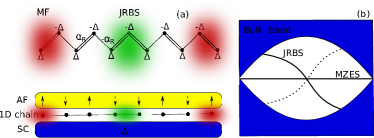
Figure 1: (Color online) (a) two 1D models we studied. In the upper model, the double bonds and single bond are used to illustrate the alternative stronger and weaker hoppings between the nearest neighboring sites. The spin-orbital interaction $\alpha_{R}$, as well as the on-site Cooper pairing $\Delta$ are also staggered along the chain. The domain-wall, simulated by two adjacent stronger bonds, can host one JRBS (green cloud), while MF appears at the geometrical ends(red cloud). In the bottom model, the s-wave superconducting pairing and antiferromagnetic (AF) order are introduced to a uniform semiconductor chain by the proximity effect. The domain-wall is simulated by an AF domain-wall. (b) A schematic illustration of the energy spectrum of bulk states, the eigen-energy of JRBS and MZES in the TSP. The blue regions represent the bulk band. The JRBS must continuously connect the particle and hole bands and inevitably go through zero energy at a point. The dotted line shows the eigen-energy of its antiparticle obeying the particle-hole symmetry.

We will show that these features could be realized in two 1D systems showed in Fig. 1 (a). The first model can be realized with cold atoms in an artificial 1D lattice with staggered nearest neighboring hopping, staggered spin orbital interaction and staggered superconducting pairing. The latter one is more easier to be carried out by sandwiching a semiconductor chain between an antiferromagnet(AF) and an ordinary s-wave superconductor. In our numerical calculation, the domain-wall is simulated by two adjacent stronger(weaker) bonds in the first model and by an AF domain-wall in the latter one. But our conclusions, in general, do no depend on the actual size and shape of the domain-walls.

In section 2, we will concentrate on the first model. Its phase diagram, the FP JRBS, the coexistence of JRBS and MF, the unavoidable zero energy crossing for JRBS and how to encode a qubit into one MZES with the help of a JRBS are discussed in this section. In section 3, we study paralleled on the second model. Section 4 is the conclusions.

II The first model

II.1 The Hamiltonian of the first model

We start from a theoretical 1D tight-binding Hamiltonian,

$$H = \sum_{i\beta}\mu c^{\dagger}_{i\beta}c_{i\beta}+\sum_{i\beta\gamma}[1-(-1)^{i}\delta](c^{\dagger}_{i+1\beta}\sigma^{z}_{\beta\gamma}c_{i\gamma}+\text{h.c.})$$ (1)

$$+\sum_{i\beta\gamma}Bc^{\dagger}_{i\beta}\sigma^{z}_{\beta\gamma}c_{i\gamma}+\alpha_{R}\sum_{i}(c^{\dagger}_{i\uparrow}c_{i+1\downarrow}-c^{\dagger}_{i\downarrow}c_{i+1\uparrow}+\text{h.c.})$$

$$+\sum_{i}\Delta(c^{\dagger}_{i\uparrow}c^{\dagger}_{i\downarrow}+\text{h.c.}).$$

Here, $c_{i\beta}$ and $c^{\dagger}_{i\beta}$ are the annihilation and creation operators for spinful fermion with spin $\beta$ on site $i$ and $\sigma$’s are Pauli matrices. The strength of hopping between the nearest neighboring sites stagger between $1+\delta$ and $1-\delta$, where the energy unit is set as the uniform part of hopping strength. Each unit cell contains the sites from the two sublattices, denoted by $A$ and $B$, respectively. $\sigma^{z}$ appears in the hopping term because we have applied a transformation, $c_{(2n+1)\downarrow}\to-c_{(2n+1)\downarrow}$, on the odd sites of the lattice for the upper model showed in Fig. 1(a). The parameters $\mu$, $\delta$, $\alpha_{R}$ and $\Delta$ are for the strength of the chemical potential, the staggered part of hopping, the staggered spin-orbital interaction and the staggered superconducting pairing, respectively.

Such Hamiltonian, Eq. 1, may be realized with cold fermions trapped in a 1D laser induced lattice. The staggered hoppings like that in the SSH model has been realized in the experimentHague and MacCormick (2012); Atala and et. al. (2012). In a recent proposal Liu et al. (2014), the staggered effective spin-orbital interaction can also be produced with the aid of modern technologies. It was also known that 1D Fermi gas with spin orbital coupling was dominated by Fulde-Ferrell (FF) superfluid phase at the low temperature Lu et al. (2012); Xu et al. (2014); Fulde and Ferrell (1964); Chen (2013). This FF phase, if properly choosing the lattice constant of the 1D lattice, can be simulated with a staggered pairing coefficient. So the tight-binding Hamiltonian of the system reads

$$H = \sum_{i\beta}\mu c^{\dagger}_{i\beta}c_{i\beta}+\sum_{i\beta}[1-(-1)^{i}\delta](c^{\dagger}_{i+1\beta}c_{i\beta}+\text{h.c.})$$

$$+\sum_{i\beta\gamma}Bc^{\dagger}_{i\beta}\sigma^{z}_{\beta\gamma}c_{i\gamma}+\sum_{i}(-1)^{i}\Delta(c^{\dagger}_{i\uparrow}c^{\dagger}_{i\downarrow}+\text{h.c.})$$

$$-\sum_{i}(-1)^{i}\alpha_{R}(c^{\dagger}_{i\uparrow}c_{i+1\downarrow}+c^{\dagger}_{i\downarrow}c_{i+1\uparrow}+\text{h.c.}),$$

where the chemical potential, the staggered hoppings, the magnetic field induced Zeeman term, the FF superfluid pairing and the staggered spin-orbital interaction are written, subsequently. Through a transformation on the odd lattice, $c_{2n+1\uparrow}\to c_{2n+1\uparrow}$ and $c_{2n+1\downarrow}\to-c_{2n+1\downarrow}$, the staggered spin-orbital and superconducting interactions are smeared out in the new representation and the Hamiltonian changes to the effective one in Eq. 1.

II.2 The phase diagram

We can study the model with the periodic boundary condition so that the wave vector $k$ is a good quantum number. The Hamiltonian in the Nambu, the spin and the sublattice representation $(\psi_{kA\uparrow},\psi_{kB\uparrow},\psi_{kA\downarrow},\psi_{kB\downarrow},\psi^{\dagger}_{-kA\uparrow},\psi^{\dagger}_{-kB\uparrow},\psi^{\dagger}_{-kA\downarrow},\psi^{\dagger}_{-kB\downarrow})^{T}$ reads

$$H(k)=\begin{pmatrix}H_{0}(k)&V(k)\\ V^{\dagger}(k)&-H_{0}(k)\end{pmatrix},$$ (3)

where

$$H_{0}(k)=\begin{pmatrix}B+\mu&(1+\delta)+(1-\delta)e^{-ik}&0&\alpha_{R}(1-e^{-ik})\\ (1+\delta)+(1-\delta)e^{ik}&B+\mu&-\alpha_{R}(1-e^{ik})&0\\ 0&-\alpha_{R}(1-e^{-ik})&-B+\mu&-[(1+\delta)+(1-\delta)e^{-ik}]\\ \alpha_{R}(1-e^{ik})&0&-[(1+\delta)+(1-\delta)e^{ik}]&-B+\mu\end{pmatrix}$$

and

$$V(k)=\begin{pmatrix}0&0&\Delta&0\\ 0&0&0&\Delta\\ -\Delta&0&0&0\\ 0&-\Delta&0&0\end{pmatrix}.$$

Through a unitary transformation

$$U=\frac{1}{\sqrt{2}}\begin{pmatrix}I&I\\ I&-I\end{pmatrix},$$

the Hamiltonian is transformed to

$$H(k)\to UH(k)U^{-1}=\begin{pmatrix}0&A(k)\\ A^{\dagger}(k)&0\end{pmatrix},$$

where $I$ is a $4\times 4$ unit matrix and $A(k)=H_{0}(k)+V(k)$.

For a gapped ring, the band gap can only close at $k=0$ or $k=\pi$ in the Brillouin zone as varying parameters. At these phase boundaries, the nonzero bulk wavefunction at $E=0$ implies $\text{det}(A)=0$. So we have the two phase boundary conditions, $B^{2}=\Delta^{2}+\mu^{2}+4\pm 4\sqrt{\Delta^{2}+\mu^{2}}$ from $k=0$ and $B^{2}=\Delta^{2}+4\delta^{2}+\mu^{2}-4\alpha^{2}\pm 4\sqrt{\Delta^{2}\delta^{2}+\delta^{2}\mu^{2}-\Delta^{2}\alpha^{2}}$ from $k=\pi$.

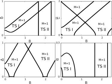
Figure 2: The phase diagram in $B-\delta$ (a) , $B-\mu$ (b), $B-\Delta$ (c) and $B-\alpha_{R}$ (d) planes. The other parameters are $\mu=0.1$, $\alpha_{R}=0.1$ and $\Delta=0.3$ in (a), $\alpha_{R}=0.1$, $\Delta=0.3$ and $\delta=0.2$ in (b), $\alpha_{R}=0.1$, $\delta=0.2$ and $\mu=0.1$ in (c) and $\delta=0.2$, $\mu=0.1$ and $\Delta=0.3$ in (d). The regions in the TSP with a topological invariant $M=1$ have been indicated explicitly. The rest regions are for topological trivial phase with $M=0$. The coexistence of MF and JRBS happens only in the TPS indicated by “TS I”.

In Fig. 2, we sketch the phase diagram in $B-\mu$, $B-\alpha$, $B-\Delta$ and $B-\delta$ planes, respectively by numerically diagonalizing $H(k)$. The phase boundaries are consistent with the above two conditions except on the $B$ axis when $\alpha=0$ or $\Delta=0$. This deviation is because in these particular conditions, the model is gapless, which violates our assumption that the gap closes at $k=0$ or $k=\pi$.

A topological invariant can be defined by $M=\frac{\Phi_{ZB}}{\pi}\,\text{mod}\,2$, where $\Phi_{ZB}$ is the Zak-Berry phase integrated over the whole Brillouin zone $\Phi_{ZB}=\int_{-\pi}^{\pi}-i\langle\psi|\partial_{k}|\psi\rangle dk$ and $|\psi\rangle$ is the eigenstate with the negative energy at $k$. The above topological invariant specified by the Zak-Berry phase is equivalent to the Pfaffian invariant first introduced by Kitaev in studying 1D topological superconductor Budich and Ardonne (2013). In Fig. 2, we indicate the regions in the topological superconducting phase (TSP) with $M=1$. The rest regions are for the topological trivial phase with $M=0$. We will show that, the phase diagram contains two kind of TSPs, denoted by “TS I” and “TS II” in the figures, respectively. MFs and JRBS can only coexist in “TS I”, a region existes only when $|\delta|>|\alpha_{R}|$, but not in “TS II” stemming from $B=2$.

These topological nontrivial phases can be confirmed by the existence of boundary states at the geometrical ends. In Fig. 3(a), we plot energy spectrum for the Hamiltonian with open boundary condition. The length of the chain is $N=400$ and the chemical potential is $\mu=0$. If not mentioned, in this paper, the spectrum show only the eigenenergies with positive energies. Their counterparts with negative energies are not explicitly shown.

Fig. 3 (a) shows that there is one Majorana zero energy state (MZES) in the band gap in two regions: “TS I” in $0.05<|B|<0.65$ and “TS II” in $1.7<|B|<2.3$. There is also another exotic region in $0.65<|B|<1.7$, where two MZESs appear. The double-degenerate Kramers MF bound states have been discussed in a two-chains model with particle-hole and time-reversal symmetry in Ref. Gaidamauskas et al. (2014); Haim et al. (2014). The two zero-energy bound states in our model are similar to this MZES pair but the time-reversal symmetry has been replaced by the sublattice symmetry when $\mu=0$.

In Fig. 3(b), we plot the energy spectrum for the model with periodic boundary condition and the length of the ring is changed to $N=401$. As the length of the unit cell is $2$, the ring contains insuppressible half unit cell. So this ring naturally engages a domain-wall and the energy spectrum exhibit the bound state at the wall. In Fig. 3(b) MZES disappears as there is no geometric end. Outside “TS I”, the energies of bound states are adjacent to the bulk band, implying that the domain-wall can only be considered as a normal impurity in that case. In “TS I”, however, a bound state deep-in-gap can evolve continuously across the zero energy. This implies that the domain-wall in “TS I” should be considered as a topological impurity that triggers one JRBS.

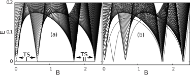
Figure 3: The energy spectrum for $N=400$ chain with open boundary condition (a) and for $N=401$ ring with periodic boundary condition (b). Only the positive eigenenergies are shown. Parameters are $\delta=0.2$, $\Delta=0.3$, $\alpha_{R}=0.1$ and $\mu=0$. In (a), a single MZES appears in two regions: “TS I” $0.05<|B|<0.65$ and “TS II” $1.7<|B|<2.3$. There are two MZESs in the region $0.65<|B|<1.7$. Panel (b) shows that a domain-wall can bring one bound state deep in band gap in “TS I”.

II.3 Another way to understand TSP when $\mu=0$

When $\mu=0$, through a unitary transformation

$$U=\frac{1}{\sqrt{2}}\begin{pmatrix}1&0&0&0&0&0&-1&0\\ 0&1&0&0&0&0&0&-1\\ 0&0&1&0&-1&0&0&0\\ 0&0&0&1&0&-1&0&0\\ 0&0&1&0&1&0&0&0\\ 0&0&0&1&0&1&0&0\\ 1&0&0&0&0&0&1&0\\ 0&1&0&0&0&0&0&1\\ \end{pmatrix},$$

the Hamiltonian can be decoupled into two partitioning parts

$$H\to UHU^{\dagger}=\begin{pmatrix}H_{+}&0\\ 0&H_{-}\end{pmatrix},$$ (4)

where

$$H_{-}=-\begin{pmatrix}B-\Delta&(1+\delta)+(1-\delta)e^{-ik}&0&\alpha_{R}(1-e^{-ik})\\ (1+\delta)+(1-\delta)e^{ik}&B-\Delta&-\alpha_{R}(1-e^{ik})&0\\ 0&-\alpha_{R}(1-e^{-ik})&-B+\Delta&-[(1+\delta)+(1-\delta)e^{-ik}]\\ \alpha_{R}(1-e^{ik})&0&-[(1+\delta)+(1-\delta)e^{ik}]&-B+\Delta\end{pmatrix}$$

and

$$H_{+}=\begin{pmatrix}B+\Delta&(1+\delta)+(1-\delta)e^{-ik}&0&\alpha_{R}(1-e^{-ik})\\ (1+\delta)+(1-\delta)e^{ik}&B+\Delta&-\alpha_{R}(1-e^{ik})&0\\ 0&-\alpha_{R}(1-e^{-ik})&-B-\Delta&-[(1+\delta)+(1-\delta)e^{-ik}]\\ \alpha_{R}(1-e^{ik})&0&-[(1+\delta)+(1-\delta)e^{ik}]&-B-\Delta\end{pmatrix}.$$

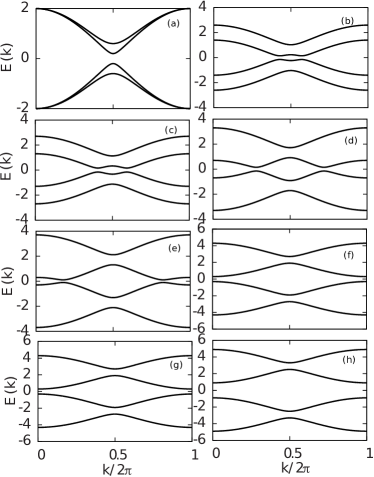
Figure 4: The band dispersion with $k$ for the two partial Hamiltonians, $H_{-}$ (a) (c) (e) (g) and $H_{+}$ (b) (d) (f) (h). The parameters are $\alpha_{R}=0.1$, $\delta=0.2$, $\Delta=0.3$ and $B=0.3$ (a) (b), $B=1$ (c) (d) $B=2$ (e) (f) and $B=2.6$ (g) (h).

We show the dispersion of the eigen-energies for the two partitioning parts, $H_{-}$ and $H_{+}$, in different phases in Fig. 4, respectively. (a), (c), (e) and (g) are for $H_{-}$ and (b), (d), (f), (h) are for $H_{+}$. The four rows of panels show the dispersion with $B=0.3$ (in “TS I”), $B=1$, $B=2$ (in “TS II”) and $B=2.6$, respectively. The band inversion happens only in one partitioning part of the Hamiltonian in “TS I” and “TS II”. This is consistent with our conclusions that “TS I” and “TS II” are in the TSP with only one MZES. The region in between I and II can host totally two MZESs, one in $H_{+}$ and the other in $H_{-}$.

II.4 Fractional parity JRBS

Next, we will use a topological argument to prove that each JRBS carries FP. From this, we can conclude that the zero energy crossing for JRBS is unavoidable. After that, the application of this property on the controllable switching of the occupation states of a MZES is presented.

We use the evolution of Wannier functions (WF) during the Thouless pump to complete a topological proof of the assertion raised in the introduction.

We extend the Thouless pump (charge pump), first introduced to the SSH model Shen (2012), to the present spinful model. It is introduced by modifying the Hamiltonian with an extra parameter $\phi$, $H(\phi)=H_{0}(\phi)+H_{\text{st}}(\phi)$, where $H_{\text{st}}(\phi)=\sum_{i}h_{\text{st}}\sin(\phi)(-1)^{i}(c^{\dagger}_{i\uparrow}c_{i\uparrow}-c^{\dagger}_{i\downarrow}c_{i\downarrow})$ and $H_{0}(\phi)$ is a modified Hamiltonian by replacing $\delta$ with $\delta\cos(\phi)$ in Eq. 1. The absolute value of $h_{\text{st}}$ is moderate so that the band gap at the Fermi energy is not closed during the pump.

The most localized WFs Thouless (1984); Thonhauser and Vanderbilt (2006); Qi (2011) for the occupied bands are obtained from the eigenvectors of the tilde position operator $\tilde{R}(\phi)=\hat{P}(\phi)\hat{R}\hat{P}(\phi)$, where $\hat{R}$ is the position operator extended to the Nambu representation and $\hat{P}(\phi)=\sum_{\alpha\in\text{occupied states}}|\alpha(\phi)\rangle\langle\alpha(\phi)|$ is the project operator on the occupied states ($E<0$) for the Hamiltonian $H(\phi)$. Here the position operator is $\hat{R}=\text{diag}(1,2,\cdots,N)\tau_{0}$, where $\tau_{0}$ is the $2\times 2$ unit matrix in the particle-hole subspace and $\text{diag}(1,2,\cdots,N)$ is a diagonal matrix with the diagonal elements running through lattice sites from $1$ to $N$. The eigenvalues of $\tilde{R}(\phi)$, denoted as $R$s, are the central positions of the WFs. It should be noticed that in the Nambu representation, each unit cell contributes $4$ WFs while in a half filled spinless SSH model, it contributes only $1$ WF.

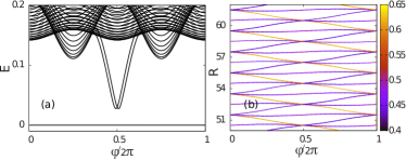
Figure 5: The energy spectrum for $H(\phi)$ with open boundary condition (a) and the associated center positions of WFs (b).The length of the chain is $N=400$. Parameters are $\delta=0.2$, $\Delta=0.3$, $\mu=0.1$ $\alpha_{R}=0.1$ and $h_{\text{st}}=0.3$. The color palette in (b) is indicating the weights of WFs projected onto the particle subspace in Nambu representation.

In Fig. 5, we plot the energy spectrum (a) and the center positions of WFs (b) during the Thouless pump with the parameters in “TS I”. The energy spectrum shows that with the moderate value of $h_{\text{st}}=0.3$, the band gap keeps open during the pump. This fact ensures that the WFs are localized and their center positions showed in (b) are reliable Kivelson (1982). According to the evolution of the center positions of WFs showed in Fig. 5(b), these WFs can be classified into two groups, one corresponding to the WFs that do not change their position after a circle of pump and the other corresponding to the WFs that change their positions by one unit cell. The WFs in the latter group can be further divided into two kinds, one(in blue) is those moving in the positive direction with $\phi$ and the other (in red) includes those moving inversely.

In the above subsection, we show that the Hamiltonian can be decoupled into two parts, $H_{\pm}$, when $\mu=0$. Increasing $\mu$ from $0$ prohibits this decoupling but the topological properties of the band keep invariant until the band gap closes. After compared Fig. 5 (b) with the evolution of the center positions of the WFs for the partitioning Hamiltonian $H_{\pm}$, shown in Fig. 6, we can conclude that the above two groups of WFs inherit the evolution with $\phi$ from those of the partial Hamiltonians $H_{\pm}$, respectively. The WFs inherited from those of $H_{+}$ experience a trival evolution (WFs come back to their initial positions) after a circle of pump while the other set that undergo a nontrivial evolution (WFs switch one unit cell) come from $H_{-}$. If transforming $H_{\pm}$ back to the lattice representation through an inverse Fourier transformation, one can find MF at the ends in $H_{+}$ and JRBS at domain-wall in $H_{-}$.

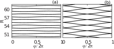
Figure 6: The evolution of the center positions of WFs during the Thouless pump for the two partitioning Hamiltonians, $H_{+}$ (a) and $H_{-}$ (b). The parameters are same as those in Fig. 5 except $\mu=0$.

We have also studied the evolution of the center positions of WFs with the parameters in “TS II”. But the WFs do not show any nontrivial evolution in that case.

Fig. 5(b) can help us recognize that each JRBS carries FP. The topological proof includes $4$ steps and we would like to highlight the goal of each step at the first. In the 1st step, besides the chains A and B raised in the introduction, an auxiliary chain C is employed. C is not uniform but with the pump parameter $\phi$ varying slowly along it from $0$ to $2\pi$. The other parameters are the same as those in the uniform chain A. From the evolution of WFs showed in Fig. 5 (b), on account of the total numbers of WFs, we can conclude that chains C and A are different by one pair of WFs. In the 2nd step, we prove that chains B and C have the same numbers of WFs. So with the bridge: chain C, we find that chains A and B are different by the pair of WFs in the number of total WFs. In the 3rd step, at a particular set of parameters, $\mu=0$, $B=0.3$ and $\alpha_{R}=0$, the pair of WFs implies that the total number of quasi-particles in A and B are different by one in the representation of $H_{\pm}$. In the 4th step, after coming back to the original Nambu representation, the above one quasi-particle difference is equivalent to the parity difference between chains A and B. When the parameters leave away from these particular ones, the above conclusion is not modified as long as they are still in “TS I”.

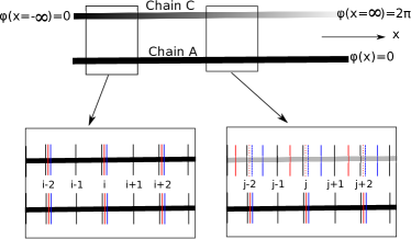
Figure 7: Chain C is describing by the extended Thouless pump Hamiltonian $H(\phi(x))$ with $\phi(x)$ slowly varying along the chain. The short vertical lines in the two zoomed pictures represent the localized WFs. There are 4 WFs in each unit cell and $i$,$j$ are used to denote the positions along the chain.

The first step.— Let us compare the center positions of WFs in the two infinite chains A and C, which are described by the Thouless pump Hamiltonian $H(\phi)$. Chain A is a uniform chain with $\phi=0$ (the Hamiltonian regresses to Eq. 1) and B is a chain on which $\phi$ is slowly varying $2\pi$ along it, which have been schematically showed in Fig. 7. Without loss of generality, we let $\phi(x=-\infty)=0$ and $\phi(x=\infty)=2\pi$ in C. Because $\phi(x)$ is varying very slowly, in each macroscopically small but microscopically large segments, it can be considered as a constant. This ensures us to find the positions of the WFs in each segment in the latter chain. For the segments at $x=-\infty$, the positions of WFs in two chains are identical. But as $x$ is increasing, compared with those in A, a set of WFs (in blue) in C begins to misalign slightly in the positive $x$ direction while another set of WFs (in red) has misaligned simultaneously in the negative direction, as showed in the figure. As we sweeping our focus through the chains from $x=-\infty$ to $x=+\infty$, the above misalignments increase and finally reach $\pm 2$, the length of a unit cell. This can be considered as that tunning on $\phi(x)$ in chain C will push a WF (in blue) outside and pull a WF (in red) inside at $x=+\infty$. So we can conclude that compared with the uniform chain, C donates one WF (in blue) and accepts another WF (in red).

The second step.— Now we relax the restriction that $\phi(x)$ is varying slowly along C. This relaxation does not affect the above conclusion because the local fluctuations of $\phi(x)$ can not distort the global property happening at $x=+\infty$. For simplicity, we let $\phi(x)$ jumps $\pi$ at two long separating points and keeps constant elsewhere. This new layout of $\phi(x)$ is just describing a chain with a pair of domain-walls, which is chain B actually. So this pair of domain-walls must take the responsibility of the pair of WFs that have been lost and gained. Because the two domain-walls are identical through a mirror reflection, their properties must be the same. So each domain-wall is in response to one half of the WF pair.

The third step.— With the particular parameters, $\mu=0$, $\delta=0.2$,$\Delta=0.3$, $B=0.3$ and $\alpha_{R}=0$, the Hamiltonian $H(k)$ can be decoupled into two parts, $H_{\pm}$. The pair of WFs that have been lost and gained comes from those of $H_{-}$. So we only need to focus on the partial Hamiltonian $H_{-}$, which has been given explicitly. In this representation, $\alpha_{R}$ is playing the role of superconducting pairing. When $\alpha_{R}=0$, this Hamiltonian regresses to a standard spinless SSH model. The dimension of $H_{-}$ has been extended from that of the standard spinless SSH model,$2\times 2$, to $4\times 4$ because a Nambu representation is still taken. The two sets of WFs, in blue and in red, come from the empty conduction band and the filled valence band of the SSH model, respectivelyXiong and Tong . So in the representation of $H_{-}$, the pair of lost and gained WFs corresponds to one quasi-particle difference.

The fourth step.— After returning back to the ordinal Nambu representation of $H(k)$, the one quasi-particle difference between A and B corresponds to the difference of the parities of fermion numbers in A and B. Tunning on $\alpha_{R}$ and $\mu$ does not disturb this conclusion because the spin-orbital interaction and chemical potential commute with particle number operator so that they also commute with the parity.

Through the above $4$ steps, we have topologically proved that the total fermion parity on chains A and B, $P_{A}$ and $P_{B}$, are different, $|P_{A}-P_{B}|=1$. So each JRBS takes the responsibility of one half of the parity difference and FP comes out naturally.

We also numerically calculate the parity of the chains A and B with length $N=400$ and periodic boundary condition. The fermion parity is calculated by $P=\text{rank}(v)\;{\text{mod}}\,2$ Ben-Shach et al. , where $\text{rank}(v)$ is the rank of Bogoliubov matrix $v$. We confirm that $|P_{A}-P_{B}|=1$ in “TS I” and $|P_{A}-P_{B}|=0$ elsewhere.

II.5 The nonuniversal average charge carried by JRBS

We have argued that, when the superconducting pairing is nonzero, JRBS should not carrying the universal fractional charge $e/2$, because the particle number is not well defined. We numerically confirm it by calculating the electric charge $Q$ (in the units of $e$) carried by a JRBS Kivelson and Schrieffer (1982),

$$Q=\rho_{L}^{\text{WD}}-\rho_{L}^{0},$$ (5)

where $\rho_{L}^{\text{WD}}$ is the average total particle number in a segment with a domain-wall at its center and $\rho_{L}^{0}$ is the average particle number for a segment without the domain-wall. $L$ is the length of these segments which should exceed the localization length of JRBS. In the numerical calculation, we choose $L=200$ which is long enough for a saturated $Q$.

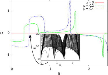
Figure 8: (Color online) Electric charge carried by a domain-wall. The system is a ring embedded with a domain-wall with the parameters, $\delta=0.2$, $\Delta=0.3$ and $\alpha_{R}=0.1$. The length of the ring is $N=401$ and the length of the segments are $L=200$. $\rho_{L}^{\text{WD}}$ and $\rho_{L}^{0}$ are numerically calculated on a half of the ring with the domain-wall at the center and on the part of the rest half (excluding one site at the end),respectively. The inset shows the energy spectrum for the ring with $\mu=0.4$. The arrow indicates the consistence of the point at where the zero energy crossing happens and electric charge $Q$ switches sign.

The electric charge $Q$ as a function of $B$ is showed in Fig. 8. It is confirmed that $Q$ becomes non-universal and is dependent on $\mu$, as well as on $B$ in “TS I”. When $\mu=0$, the domain-wall becomes neutral because the particle number on each site is exactly one, independent of the presence of domain-wall. When $\mu\neq 0$, the nonzero $Q$ is smoothly varying in “TS I”, except near a $B_{0}$ at which its sign is switched. This sign switching is directly associated with the zero energy crossing for JRBS showed in the inset. In inset, we show the energy spectrum for the ring with $\mu=0.4$. The eigen-energy inside the bulk gap is for the JRBS on domain-wall. It is the particle-hole transition for the JRBS around the zero energy crossing point that changes the sign of electrical charge $Q$.

In “TS II”, the charge shows a peak and a dip at the phase boundaries. But it is almost zero in the region. We suggest that the peak and dip are due to the quantum fluctuation accompanied with the band gap closing.

II.6 Unavoidable zero energy crossing

The energy spectrum in inset of Fig. 8 (as well as in Fig. 3) shows a zero energy crossing for JRBS. Now we apply a topological argument to prove that the zero energy crossing is unavoidable. We start from a proof by contradiction by supposing that the energy spectrum for JRBS does not cross zero energy. If that is ture, one can modify factors, i.e., the size of the domain-wall, to continuously change its eigen-energy from deep-in-gap to near the bulk band. In this case, the eigenenergy of JRBS is not different from that of a normal impurity. When embedding such a domain-wall in a uniform chain, its contribution of fermion parity is fixed, either $0$ or $1$. When the embedded domain-walls become two, their total contributions of fermion parity become $0$. But as we have showed, $|P_{A}-P_{B}|=1$, which requires that the two JRBSs must contribute an extra fermion parity. Here, we get the contradicting results so that the initial assumption must be wrong. So the FP JRBS in “TS I” must trigger an eigenstate with its eigenenergy crossing the zero energy inevitably.

One can confirm the robustness of the crossing by studying a disordered lattice. Here we study a model with the disordered hopping integral between the nearest neighboring sites, $\delta_{i}=\delta(1+w_{i})$, where $\delta=0.2$ and $w_{i}$ is randomly distributing in $[-0.6,0.6]$. The spectrum is showed in Fig. 9. It shows that the zero energy crossing for the eigenenergy of JRBS is robust against the lattice distortion.

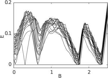
Figure 9: The energy spectrum for a disordered lattice. The parameters are the same as those in Fig. 3. The disordered system is a $N=401$ chain with open boundary condition and embedded by a domain-wall at the center.

II.7 Majorana Fermion and JRBS

In the previous discussion, our focus is on JRBS. In this subsection, we show the coexistence of MF and JRBS and how to switch between the empty state and the occupied state of MZES with the help of JRBS.

In Fig. 10, we show the typical energy spectrum for an open chain embedded with a domain-wall at the center. In “TS I”, the persistent zero energy state is MZES and the nonzero eigen-energy of JRBS crosses the zero energy at $B_{0}$. As showed explicitly in the figure, the wave-functions of these states are localized at the domain-wall for JRBS and at the geometrical ends for MZES.

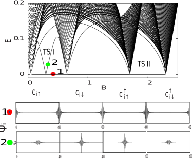
Figure 10: (Color online) Upper panel: energy spectrum for the chain embedded with a domain-wall. Lower panel: amplitudes of wavefunctions of MZES and JRBS in representation $(c_{i\uparrow},c_{i\downarrow},c^{\dagger}_{i\uparrow},c^{\dagger}_{i\downarrow})^{T}$, where $i$ runs through the lattice sites from $1$ to $N=401$. The other parameters are the same as those in Fig. 8 except $\mu=0$.

When we ignore the MZES by modifying the geometry of the model from chain to ring (no geometrical ends). It is known that the fermion parity of ground state of the ring is changed when $B$ is varying across $B_{0}$ because of the zero energy crossing. This is confirmed by the numerical calculation on the parity of the ring. So the ground states on $B<B_{0}$ and $B>B_{0}$ in “TS I” have different fermion parity. Therefore, if we increase $B$ to cross $B_{0}$ with a ring at its ground state initially, the final state must be an excited state and can not spontaneously jump back to the final ground state because the parity is conserved in this process.

When the MZES is reconsidered in a chain, the above excited state can jump back to the final ground state by a parity compensation on MZES. This compensation is achieved by the switching between the empty state and the occupied state of MZES because this switching contributes one parity change. In this manner, with the help of a JRBS embedded in the chain, we would be able to flip between the two states of the MZES still in the restriction that the total fermion parity is conserved. A quantum qubit can be encoded into these two states of one MZES, while in chains without JRBS, two MZESs are needed.

III The second model with local AF order.

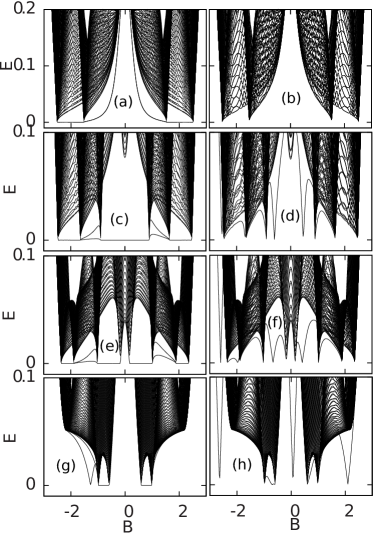
Figure 11: The energy spectrum for a $N=400$ chain with open boundary condition (left column) and for a $N=401$ ring with an AF domai-wall (right column). The parameters are $\theta=0.6$, $\Delta=0.3$ and $\alpha_{R}=0.1$ in these panels. $M$ is $0$ (a) (b), $0.5$ (c) (d), $0.8$ (e) (f) and $1$ (g) (h).

The Hamiltonian reads,

$$H = \sum_{i\beta}[(c^{\dagger}_{i\beta}c_{i+1\beta}+\text{h.c.})+\mu c^{\dagger}_{i\beta}c_{i\beta}]$$ (6)

$$+i\alpha_{R}\sum_{i\beta\gamma}(c^{\dagger}_{i\beta}\sigma^{y}_{\beta\gamma}c_{i+1\gamma}+\text{h.c.})$$

$$+\sum_{i\beta\gamma}c^{\dagger}_{i\beta}(\vec{B}-\vec{M}_{i})\cdot\vec{\sigma}_{\beta\gamma}c_{i\gamma}$$

$$+\Delta\sum_{i}(c^{\dagger}_{i\uparrow}c^{\dagger}_{i\downarrow}+\text{h.c.}),$$

where hopping, chemical potential, spin-orbital interaction, Zeeman interaction caused by a uniform magnetic field $\vec{B}$ and staggered local magnetic momenta $\vec{M}_{i}$ and s-wave superconducting pairing are expressed, respectively. We fix the magnetic field in the $x-z$ plane with $\vec{B}=\sin(\theta)B\hat{z}+\cos(\theta)B\hat{x}$ and the staggered local AF momenta are in the $x$ direction, $\vec{M}_{i}=(-1)^{i}M\hat{x}$.

In experiment, AF magnetic order and s-wave superconducting pairing can be introduced to a 1D semi-conductor through proximity effect by sandwiching it with AF material and superconductor.

This Hamiltonian in the momentum space in the representation of the sublattice, the spin and the particle-hole subspaces ,$(\psi_{kA\uparrow},\psi_{kB\uparrow},\psi_{kA\downarrow},\psi_{kB\downarrow},\psi^{\dagger}_{-kA\uparrow},\psi^{\dagger}_{-kB\uparrow},\psi^{\dagger}_{-kA\downarrow},\psi^{\dagger}_{-kB\downarrow})^{T}$, reads

$$H=\begin{pmatrix}H_{0}&V\\ V^{\dagger}&-H_{0}\end{pmatrix},$$ (7)

where

$$H_{0}=\begin{pmatrix}\mu+B\sin(\theta)&1+e^{-ik}&B\cos(\theta)+M&\alpha_{R}(1-e^{-ik})\\ 1+e^{ik}&\mu+B\sin(\theta)&-\alpha_{R}(1-e^{ik})&B\cos(\theta)-M\\ B\cos(\theta)+M&-\alpha_{R}(1-e^{-ik})&\mu-B\sin(\theta)&1+e^{-ik}\\ \alpha_{R}(1-e^{ik})&B\cos(\theta)-M&1+e^{ik}&\mu-B\sin(\theta)\end{pmatrix},$$

and

$$V=\begin{pmatrix}0&0&\Delta&0\\ 0&0&0&\Delta\\ -\Delta&0&0&0\\ 0&-\Delta&0&0\end{pmatrix}.$$

When $\mu=0$, the above Hamiltonian can also be decoupled into two partitioning parts,

$$H\to\begin{pmatrix}H_{+}&0\\ 0&H_{-}\end{pmatrix},$$ (8)

where

$$H_{+}=\begin{pmatrix}B\sin(\theta)+\Delta&1+e^{-ik}&B\cos(\theta)+M&\alpha_{R}(1-e^{-ik})\\ 1+e^{ik}&B\sin(\theta)-\Delta&-\alpha_{R}(1-e^{ik})&B\cos(\theta)-M\\ B\cos(\theta)+M&-\alpha_{R}(1-e^{-ik})&\Delta-B\sin(\theta)&1+e^{-ik}\\ \alpha_{R}(1-e^{ik})&B\cos(\theta)-M&1+e^{ik}&-B\sin(\theta)-\Delta\end{pmatrix}$$

and $H_{-}=-H_{+}$ after a unitary transformation

$$U=\frac{1}{\sqrt{2}}\begin{pmatrix}1&0&0&0&0&0&-1&0\\ 0&1&0&0&0&0&0&1\\ 0&0&1&0&1&0&0&0\\ 0&0&0&1&0&-1&0&0\\ 0&0&-1&0&1&0&0&0\\ 0&0&0&1&0&1&0&0\\ 1&0&0&0&0&0&1&0\\ 0&-1&0&0&0&0&0&1\\ \end{pmatrix}$$

So when $\mu=0$, phase transition happens at the points $M^{2}=B^{2}\cos(2\theta)+\Delta^{2}-4\pm 2\sqrt{-B^{4}\cos^{2}(\theta)\sin^{2}(\theta)+B^{2}\Delta^{2}\cos^{2}(\theta)+4B^{2}\sin^{2}(\theta)-4\Delta^{2}}$ and $M^{2}=B^{2}\cos(2\theta)+4\alpha^{2}_{R}+\Delta^{2}-2B\sqrt{-B^{2}\cos^{2}(\theta)\sin^{2}(\theta)+\Delta^{2}\cos^{2}(\theta)-4\alpha^{2}_{R}\sin^{2}(\theta)}$.

In Fig. 11 we plot the energy spectrum for a chain with open boundary condition (left column) and for a ring with one AF domain-wall on it (right column). Like that in the first model, the AF domain-wall is simulated by two adjacent $M_{i}$s pointing to the same direction. We find in the cases (c), (d), (e) and (f), there is a TSP in which a MF zero energy bound state can coexist with a JRBS. These properties are the same as those showed for the first model.

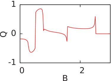
Figure 12: The electric charge carried by an AF domain-wall. The parameters are $\theta=0.6$, $\Delta=0.3$, $\alpha_{R}=0.1$ and $M=0.2$.

We numerically calculate the electric charge carried by an AF domain-wall. As Fig. 12 shows, it is non-universal just as that in the first model. We also numerically calculate the parities of fermion numbers for chains like A and B. The result is same as that in the first model. So the JRBS attached to the AF domain-wall in this model is also carrying FP. As we have discussed in the previous model, this means that the eigenenergy of JRBS must suffer an unavoidable zero energy crossing.

IV Conclusions

We have showed that JRBS and MF can coexist in a TSP in 1D models. The eigen-energy of the FP JRBS suffers an unavoidable zero energy crossing. This crossing separates the TSP into two parts with different parities for the ground state. This can be used to switch between the occupied and the empty states of MZES under the conservation of total fermion parity. One should be able to observe such effect by measuring the Josephson current through MZES. As the magnetic field is modified across the crossing point, the Josephson current should suffer a sudden sign jump because the parity on the MZES is changed. It still remains challenging how to experimentally observe the FP JRBS directly. One possible way is to apply the proposal in Ref. Rainis et al. (2014), although the electric charge on the domain-wall is not $e/2$ in this case.

Acknowledgments.— The work was supported by the State Key Program for Basic Research of China (Grant Nos. 2009CB929504, 2009CB929501), National Foundation of Natural Science in China Grant Nos. 10704040, 11175087.

References

- Ivanov (2001) D.A. Ivanov, Phys. Rev. Lett. 86, 268 (2001), ISSN 0031-9007.
- Qi and Zhang (2011) X.-L. Qi and S.-C. Zhang, Rev. Mod. Phys. 83, 1057 (2011).
- Nayak et al. (2008) C. Nayak, S. H. Simon, A. Stern, M. Freedman, and S. Das Sarma, Rev. Mod. Phys. 80, 1083 (2008).
- Liu et al. (2014) X.-J. Liu, K.T. Law, and T.K. Ng , Phys. Rev. Lett. 112, 086401 (2014).
- Fu and Kane (2008) L. Fu and C. L. Kane, Phys. Rev. Lett. 100, 096407 (2008).
- Qi et al. (2010) X.-L. Qi, T. L. Hughes, and S.-C. Zhang, Phys. Rev. B 82, 184516 (2010).
- Yan et al. (2011) X.-W. Yan, M. Gao, Z.-Y. Lu, and T. Xiang, Phys. Rev. B 84, 054502 (2011).
- Tanaka et al. (2012) Y. Tanaka, M. Sato, and N. Nagaosa, Journal of the Physical Society of Japan 81, 011013 (2012).
- He et al. (2014) J. J. He, T.K. Ng, P. A. Lee, and K.T. Law, Phys. Rev. Lett. 112, 037001 (2014).
- Kitaev (2001) A. Y. Kitaev, Phys. Usp. 44, 131 (2001).
- Sau et al. (2010) J. D. Sau, R. M. Lutchyn, S. Tewari, and S. Das Sarma, Phys. Rev. Lett. 104, 040502 (2010).
- Shen (2012) S.-Q. Shen, Topological Insulators, Dirac Equation in Condensed Matters (Springer Series in Solid-State Science 174, 2012).
- Klinovaja et al. (2012) J. Klinovaja, P. Stano, and D. Loss, Phys. Rev. Lett. 109, 236801 (2012).
- Potter and Lee (2010) A. C. Potter and P. A. Lee, Phys. Rev. Lett. 105, 227003 (2010).
- Wakatsuki et al. (2014) R. Wakatsuki, M. Ezawa, Y. Tanaka, and N. Nagaosa, Phys. Rev. B 90, 014505 (2014).
- Hasan and Kane (2010) M. Z. Hasan and C. L. Kane, Rev. Mod. Phys. 82, 3045 (2010).
- Jackiw and Rebbi (1976) R. Jackiw and C. Rebbi, Phys. Rev. D 13, 3398 (1976).
- Su et al. (1979) W. P. Su, J. R. Schrieffer, and A. J. Heeger, Phys. Rev. Lett. 42, 1698 (1979).
- Su et al. (1980) W. P. Su, J. R. Schrieffer, and A. J. Heeger, Phys. Rev. B 22, 2099 (1980).
- Kivelson and Schrieffer (1982) S. Kivelson and J. R. Schrieffer, Phys. Rev. B 25, 6447 (1982).
- Gangadharaiah et al. (2012) S. Gangadharaiah, L. Trifunovic, and D. Loss, Phys. Rev. Lett. 108, 136803 (2012).
- Rainis et al. (2014) D. Rainis, A. Saha, J. Klinovaja, L. Trifunovic, and D. Loss, Phys. Rev. Lett. 112, 196803 (2014).
- Väyrynen and Ojanen (2011) J. I. Väyrynen and T. Ojanen, Phys. Rev. Lett. 107, 166804 (2011).
- Klinovaja and Loss (2013) J. Klinovaja and D. Loss, Phys. Rev. Lett. 110, 126402 (2013).
- Hague and MacCormick (2012) J. P. Hague and C. MacCormick, New J. of Phys. 14, 033019 (2012).
- Atala and et. al. (2012) M. Atala and et. al., arXiv:1212.0572 (2012).
- Lu et al. (2012) H. Lu, L. O. Baksmaty, C. J. Bolech, and H. Pu, Phys. Rev. Lett. 108, 225302 (2012).
- Xu et al. (2014) Y. Xu, R.-L. Chu, and C. Zhang, Phys. Rev. Lett. 112, 136402 (2014).
- Fulde and Ferrell (1964) P. Fulde and R. A. Ferrell, Phys. Rev. 135, A550 (1964).
- Chen (2013) C. Chen, Phys. Rev. Lett. 111, 235302 (2013).
- Budich and Ardonne (2013) J. C. Budich and E. Ardonne, Phys. Rev. B 88, 075419 (2013).
- Gaidamauskas et al. (2014) E. Gaidamauskas, J. Paaske, and K. Flensberg, Phys. Rev. Lett. 112, 126402 (2014).
- Haim et al. (2014) A. Haim, A. Keselman, E. Berg, and Y. Oreg, Phys. Rev. B 89, 220504 (2014), URL http://link.aps.org/doi/10.1103/PhysRevB.89.220504.
- Thouless (1984) D. Thouless, J. Phys. C 17, L325 (1984).
- Thonhauser and Vanderbilt (2006) T. Thonhauser and D. Vanderbilt, Phys. Rev. B 74, 235111 (2006).
- Qi (2011) X.-L. Qi, Phys. Rev. Lett. 107, 126803 (2011).
- Kivelson (1982) S. Kivelson, Phys. Rev. B 26, 4269 (1982).
- (38) Y. Xiong and P. Tong, arXiv:1406.5568.
- (39) G. Ben-Shach, A. Haim, I. Appelbaum, Y. Oreg, A. Yacoby, and B. I. Halperin, arXiv:1406.5172.