Multiple Gluon Exchange Webs

Abstract

Webs are weighted sets of Feynman diagrams which build up the logarithms of correlators of Wilson lines, and provide the ingredients for the computation of the soft anomalous dimension. We present a general analysis of multiple gluon exchange webs (MGEWs) in correlators of semi-infinite non-lightlike Wilson lines, as functions of the exponentials of the Minkowski cusp angles, $\alpha_{ij}$, formed between lines $i$ and $j$. We compute a range of webs in this class, connecting up to five Wilson lines through four loops, we give an all-loop result for a special class of diagrams, and we discover a new kind of relation between webs connecting different numbers of Wilson lines, based on taking collinear limits. Our results support recent conjectures, stating that the contribution of any MGEW to the soft anomalous dimension is a sum of products of polylogarithms, each depending on a single cusp angle, and such that their symbol alphabet is restricted to $\alpha_{ij}$ and $1-\alpha_{ij}^{2}$. Finally, we construct a simple basis of functions, defined through a one-dimensional integral representation in terms of powers of logarithms, which has all the expected analytic properties. This basis allows us to compactly express the results of all MGEWs computed so far, and we conjecture that it is sufficient for expressing all MGEWs at any loop order.

Edinburgh 2014/12

1 Introduction

Infrared singularities of scattering amplitudes in non-Abelian gauge theories are essential for understanding the physics of the strong interactions. Determining infrared singularities is necessary in order to combine real and virtual corrections in cross section calculations. These singularities also dictate the structure of large logarithmic contributions in perturbation theory, which must in many cases be resummed in order to obtain reliable phenomenological predictions. Besides their significance to phenomenology, infrared singularities are very interesting from a theoretical perspective: first of all, they have a similar structure across all gauge theories; furthermore, their relative simplicity Catani:1998bh ; Sterman:2002qn ; Aybat:2006wq ; Aybat:2006mz ; Becher:2009cu ; Becher:2009qa ; Gardi:2009qi , their exponentiation properties Yennie:1961ad ; Sterman:1981jc ; Gatheral:1983cz ; Frenkel:1984pz ; Magnea:1990zb ; Magnea:2000ss ; Gardi:2010rn ; Mitov:2010rp ; Gardi:2011wa ; Gardi:2011yz ; Dukes:2013wa ; Dukes:2013gea ; Gardi:2013ita , and their relation with the renormalization properties of Wilson line correlators Polyakov:1980ca ; Arefeva:1980zd ; Dotsenko:1979wb ; Brandt:1981kf ; Korchemsky:1985xj ; Korchemsky:1985xu ; Korchemsky:1987wg allow us to explore multi-loop and even all-order properties, which are beyond reach when studying complete scattering amplitudes. In ${\cal N}=4$ supersymmetric Yang-Mills theory, where much contemporary focus is on the planar limit, infrared singularities give access to non-planar effects (see, for example, Refs. Naculich:2009cv ; Naculich:2011pd ; Naculich:2013xa ), and they provide a link between the weak and strong coupling regimes Alday:2007hr ; Basso:2007wd ; Correa:2012nk ; Henn:2012qz ; Correa:2012at ; Henn:2013wfa ; Erdogan:2011yc ; Cherednikov:2012yd ; Cherednikov:2012qq .

It is by now well understood that infrared divergent contributions to scattering amplitudes are universal, and can be mapped Korchemsky:1985xj to ultraviolet divergences of correlators of Wilson line operators, which have been extensively studied both in gauge and gravity theories Korchemsky:1985xu ; Korchemsky:1987wg ; Korchemsky:1985xj ; Brandt:1981kf ; Korchemsky:1992xv ; Korchemsky:1993uz ; Korchemskaya:1994qp ; Korchemskaya:1992je ; Akhoury:2011kq ; Naculich:2011ry ; Miller:2012an ; White:2011yy ; Melville:2013qca . For fixed-angle scattering amplitudes, which are the focus of the present paper, these correlators involve semi-infinite Wilson lines, pointing in the directions defined by the classical trajectories of the hard partons participating in the scattering. The renormalisation properties of such operators are encoded in the soft anomalous dimension, which is a matrix in the space of colour configurations available for the scattering process at hand. In processes involving only two Wilson lines, this reduces to the well-known cusp anomalous dimension, which is a function of the Minkowski angle between the two lines. In QCD, this function has been calculated up to two-loop order Korchemsky:1987wg (see also Kidonakis:2009ev ), and progress towards a three loop result was reported in Ref. Grozin:2014axa . In ${\cal N}=4$ Super-Yang-Mills theory it is known to three loops Correa:2012nk ; Correa:2012at , and partial results have been recently obtained at four loops Henn:2012qz ; Henn:2013wfa . For multi-parton amplitudes, the soft anomalous dimension has been calculated up to two-loop order for both massless Aybat:2006wq ; Aybat:2006mz and massive Ferroglia:2009ep ; Ferroglia:2009ii ; Mitov:2010xw ; Chien:2011wz Wilson lines (see also Mitov:2009sv ; Becher:2009kw ; Beneke:2009rj ; Czakon:2009zw ; Chiu:2009mg ; Ferroglia:2010mi ; Gardi:2013saa ).

In the case of massless partons, the two-loop result Aybat:2006wq ; Aybat:2006mz turns out to be remarkably simple, replicating the colour-dipole structure of the one-loop correction. This motivated further investigations, which led to a compact ansatz (the dipole formula) for the all-order structure of infrared singularities in massless gauge theories Becher:2009cu ; Becher:2009qa ; Gardi:2009qi . The dipole formula can only receive corrections starting at three loops, with at least four hard partons. The nature of these corrections was investigated in Dixon:2008gr ; Gardi:2009qi ; Dixon:2009gx ; Becher:2009cu ; Becher:2009qa ; Dixon:2009ur ; Gardi:2009zv ; Gehrmann:2010ue ; Bret:2011xm ; DelDuca:2011ae ; Ahrens:2012qz ; Naculich:2013xa ; Caron-Huot:2013fea , where they were shown to be highly constrained by non-Abelian exponentiation and Bose symmetry, as well as by the known behaviours of amplitudes in collinear limits and in the Regge limit Bret:2011xm ; DelDuca:2011ae ; DelDuca:2013ara ; recently, the first evidence for a non-vanishing correction to the dipole formula at the four-loop level was inferred in Ref. Caron-Huot:2013fea , using the Regge limit.

In the massive case, much of this simplicity is lost, as ‘colour tripole’ corrections, which are forbidden to all loops in the massless case, are present already at the two-loop level Ferroglia:2009ep ; Ferroglia:2009ii ; Mitov:2010xw . The result for the soft anomalous dimension retains however interesting features, in particular it has a factorized form as a function of the Minkowski angles between Wilson lines. The massless limit, where the tripole correction vanishes, involves a subtle cancellation between different diagrammatic contributions, which have different analytic behaviour in the massive case.

In order to understand the structure of infrared divergences of both massive and massless partons at three loops and beyond, it is ultimately necessary to tackle the direct calculation of correlators of multiple Wilson lines at the multi-loop level. Such correlators exponentiate, and it is then clearly beneficial to be able to calculate the exponent of the correlator directly. This problem has been addressed over the past few years in a series of papers Laenen:2008gt ; Mitov:2010rp ; Gardi:2010rn ; Gardi:2011wa ; Gardi:2011yz ; Gardi:2013ita ; Gardi:2013saa (see also Vladimirov:2014wga ), which have developed a diagrammatic approach to the non-Abelian exponentiation of products of Wilson lines. It is then also necessary to develop techniques for carrying out the relevant Feynman integrals. Recently, there has been significant progress in this direction using configuration-space techniques both for strictly lightlike Wilson lines Erdogan:2011yc and for non-lightlike lines Henn:2012qz ; Henn:2013wfa ; Gardi:2013saa ; Grozin:2014axa . The first three-loop results involving multiple Wilson lines have been published in Ref. Gardi:2013saa , where a class of diagrams contributing to the four-line soft anomalous dimension were evaluated. This also constitutes a step towards the determination of the three-loop soft anomalous dimension. In parallel progress has been made also on other three-loop diagrams Gardi:2014kpa and the complete result in the lightlike limit will soon be available.

The diagrammatic approach to exponentiation can be summarized as follows. Correlators of multiple Wilson lines exponentiate, and their logarithms can be computed directly in terms of webs. The concept of web was introduced in formulating the non-Abelian exponentiation theorem in the simpler case of a Wilson loop (or two Wilson lines meeting at a cusp) in Refs. Gatheral:1983cz ; Frenkel:1984pz ; Sterman:1981jc . In this case the diagrams that contribute to the exponent are irreducible: their colour factors cannot be decomposed into products of colour factors of their subdiagrams. Importantly, irreducible diagrams are also free of ultraviolet subdivergences associated with the renormalization of the cusp. For multiple Wilson lines this classification does not hold: reducible diagrams do contribute to the exponent. Consequently, the concept of web has to be substantially generalised. This was done in Refs. Gardi:2010rn ; Mitov:2010rp ; Gardi:2011wa ; Gardi:2011yz ; Gardi:2013ita ; Gardi:2013saa , which generalised the non-Abelian exponentiation theorem to the multi-line case. Each web $W$ then comprises a set of Feynman diagrams $\{D\}$, which is closed under permutations of the gluon attachments to the Wilson lines; writing each diagram $D$ as a product ${\cal F}(D)C(D)$, where $C(D)$ is the colour factor and ${\cal F}(D)$ is the kinematic integral, one finds that the contribution of each web to the logarithm of the Wilson line correlator is given by

$$W\,=\,\sum_{D,D^{\prime}\in W}{\cal F}(D)\,R_{DD^{\prime}}\,C(D^{\prime})\,,$$ (1)

where the sum is over all pairs of diagrams $D$ and $D^{\prime}$ belonging to the web $W$. Kinematic and colour factors of individual diagrams mix with each other according to a web-mixing matrix $R_{DD^{\prime}}$, whose entries are rational numbers of purely combinatorial origin. Furthermore, as shown in Ref. Gardi:2013ita , the linear combinations of colour factors generated through the action of the mixing matrix in eq. (1) always correspond to connected graphs. This is the essence of the non-Abelian exponentiation theorem for multiple Wilson lines.

The calculation of the logarithm of a Wilson-line correlator at a given order in perturbation theory proceeds then by classifying the possible webs, identifying which connected colour factors they contribute to, and finally computing the corresponding kinematic integrals. The goal of the calculation is identifying the ultraviolet singularities which contribute to the anomalous dimension. This, in turn, requires introducing an infrared regulator, which can be achieved using an exponential suppression of long-distance interactions with the Wilson lines, as proposed in Gardi:2011wa ; Gardi:2013saa . Renormalization, and the non-commuting nature of the colour factors, imply that each web enters the anomalous dimension together with counterterms which remove its subdivergences Mitov:2010rp ; Gardi:2010rn ; Gardi:2011wa ; Gardi:2011yz . The relevant combinations that determine the anomalous dimension were called subtracted webs in Gardi:2013saa ; these integrals have just a single ultraviolet pole, and they play the same role that individual webs play in the two-line case. As a consequence, subtracted webs are independent of the infrared regulator, and they share the same symmetries as the anomalous dimension Gardi:2013saa . A notable example of this is crossing symmetry, which is broken by the infrared regulator for non-subtracted webs, but is restored for subtracted webs. As a consequence, subtracted webs evaluate to much simpler analytic functions as compared to the individual diagrams (or the non-subtracted webs) which build them. There is therefore a marked advantage in organising the calculation in such a way that the last integrations be performed at the level of subtracted webs, as advocated in Ref. Gardi:2013saa .

In this paper we will discuss in detail the simplest class of webs contributing to multiple Wilson line correlators. These were dubbed “Multiple Gluon Exchange Webs” (MGEWs) in Ref. Gardi:2013saa , where some of their properties were studied, and two non-trivial three-loop examples were computed. MGEWs can be characterized in general as those webs that arise when the Wilson line correlator is computed using only the quadratic part of the quantum Yang-Mills Lagrangian in the path integral. In diagrammatic terms, they consist of graphs where all gluons attach directly to the Wilson lines, with no interaction vertices located off the Wilson lines. The graphs generated in this way are Abelian-like, in the sense that they would also appear in QED, however there is an essential difference between the two cases: in QED the order of emission from the Wilson lines is immaterial, and one can easily show that MGEWs collectively reconstruct powers of the one-loop result; indeed, according to the exponentiation theorem, MGE diagrams are not part of the exponent in QED. In contrast, in a non-Abelian theory the ordering of gluon emission is crucial, and, as a consequence, MGEWs contribute to the exponent, where they collectively generate fully connected colour factors.

Some key features of MGEWs were uncovered in Ref. Gardi:2013saa , based on a general analysis of the structure of their kinematic integrals, along with some physically motivated considerations concerning their analytic properties. Most notably, it was found that subtracted MGEWs can be expressed as sums of products of functions depending on individual cusp angles. The analytic structure of these functions is best elucidated by introducing, for each pair of Wilson lines $\{i,j\}$, variables $\alpha_{ij}$, corresponding to the exponential of the cusp angle $\xi_{ij}$ between the two lines, so that

$$\xi_{ij}\,=\,\ln\alpha_{ij}\,=\,\cosh^{-1}\left(-\frac{\gamma_{ij}}{2}\right)\,,\qquad\qquad\gamma_{ij}\,=\,-\,\alpha_{ij}-\frac{1}{\alpha_{ij}}\,,$$ (2)

where $\gamma_{ij}$ is defined as the normalized scalar product between the 4-velocities of the two Wilson lines, $\beta_{i}$ and $\beta_{j}$,

$$\gamma_{ij}\,\equiv\,\frac{2\beta_{i}\cdot\beta_{j}+{\rm i}\varepsilon}{\sqrt{\beta_{i}^{2}-{\rm i}\varepsilon}\sqrt{\beta_{j}^{2}-{\rm i}\varepsilon}}\,=\,\frac{2p_{i}\cdot p_{j}+{\rm i}\varepsilon}{\sqrt{p_{i}^{2}-{\rm i}\varepsilon}\sqrt{p_{j}^{2}-{\rm i}\varepsilon}}\,.$$ (3)

Here in the second equality we restored the dimensionful momenta of the partons represented by the Wilson lines, and we specified how kinematic invariants should be analytically continued.

The results for the subtracted webs considered in Ref. Gardi:2013saa were expressed in terms of a highly constrained set of functions, consisting of products of polylogarithms, each depending on a single $\alpha_{ij}$. The analytic structure of these functions has been elucidated using the symbol map Goncharov.A.B.:2009tja ; Goncharov:2010jf ; Duhr:2011zq ; Duhr:2012fh : it was conjectured that the symbols of the functions entering subtracted MGEWs are built out of the restricted alphabet $\{\alpha_{ij},\eta_{ij}\equiv\alpha_{ij}/(1-\alpha_{ij}^{2})\}$. This alphabet, in particular, realises crossing symmetry, which in this case is expressed by the reflection $\alpha_{ij}\to-\alpha_{ij}$. It is clear that, whilst all relevant integrals can be evaluated without going through the symbol map, its use is nevertheless invaluable in simplifying results and understanding their analytic structure.

The primary aim of this paper is to study the all-order structure of MGEWs in further detail, and to test the conjectures of Ref. Gardi:2013saa in a broader range of examples. Specifically, the subset of webs computed in Ref. Gardi:2013saa , connecting the maximal number of Wilson lines accessible at two and three loops, yields integrals which are less entangled than certain MGEWs connecting a smaller number of lines at the same order; the latter, more entangled ones, are computed and analysed here in order to confirm the conjectures. With the more complete understanding of MGEWs we gain here we are able to construct an ansatz for an all-order basis of functions. These are defined through one-dimensional integrals of powers of logarithms only. This yields a very restricted set of harmonic polylogarithms Remiddi:1999ew satisfying the alphabet conjecture and other constraints. We show that this basis is sufficient to express all the subtracted webs we compute in a compact manner, and we argue that it should be sufficient for MGEWs at higher orders as well.

The structure of the paper is as follows. Sec. 2 begins by reviewing the method to compute the soft-anomalous dimension using subtracted webs; we keep this discussion brief and we refer the reader to Refs. Gardi:2011yz ; Gardi:2013ita ; Gardi:2013saa for a more detailed account. In the final part of Sec. 2 we discuss the colour structure of webs using the effective vertex formulation developed in Ref. Gardi:2013ita , and identify a new type of relations between webs comprising different numbers of Wilson lines, through a process of collinear reduction. Examples of this procedure will be given later on in the paper, where it is used as a check of the results of specific webs. Then, in Sec. 3, we provide a general characterization of MGEWs: we give an integral representation valid for any web in this class, before subtraction, in terms of variables with a transparent physical interpretation, and we review the conjectures proposed in Gardi:2013saa . In Sec. 4, we explain how the basis of functions for MGEWs is constructed, and provide the necessary definitions, which will be used in what follows to express the results of the various MGEWs we compute. In the subsequent sections, we provide explicit calculations of MGEWs to substantiate our arguments; the results are also important as ingredients for the computation of the soft anomalous dimension at three loops and beyond. In Sections 4.2 and 5 we consider three-loop webs connecting two and three Wilson lines: the two-line case, already studied in Henn:2013wfa , is interesting in this context since it provides an example of maximal entanglement of gluon insertions at this order. The results of Sect. 5 constitute another significant step forward in constructing the complete three-loop soft anomalous dimension, as well as providing an interesting comparison with the four line case of Ref. Gardi:2013saa . In Sec. 6, we provide for the first time the complete calculation of a four-loop subtracted web, connecting five Wilson lines. The result is in complete agreement with the conjectured all-order properties of MGEWs. Finally, in Sec. 7, we show that a specific class of highly symmetric diagrams contributing to $n$-line webs can be explicitly computed for any $n$, obtaining a remarkably simple result that further substantiates our conjectures. This all-order calculation of kinematic factors further allows us to prove that a specific colour structure arising from these webs has a vanishing coefficient for any $n$. We discuss our results and conclude in Sec. 8, while some technical details concerning the calculation of the subtracted webs that we have presented are collected in appendices.

2 Webs and the soft anomalous dimension

We begin by summarising the formalism which will be used in what follows to determine the soft anomalous dimension from webs. For a complete discussion of this material, the reader is referred to Refs. Gardi:2011yz ; Gardi:2013saa . In Sec. 2.2 we discuss the colour structure of webs using the effective vertex formulation developed in Ref. Gardi:2013ita . This section already contains some new results: we identify there a new type of relation between webs comprising different numbers of Wilson lines, through a process of collinear reduction. These relations will provide non-trivial checks of explicit calculations in the following sections.

2.1 From webs to the soft anomalous dimension

We consider the vacuum expectation value of a product of $L$ semi-infinite Wilson lines operators, of the form

$${\cal S}\left(\gamma_{ij},\alpha_{s}(\mu),\epsilon,\frac{m}{\mu}\right)\,\equiv\,\left\langle 0\left|\Phi_{\beta_{1}}^{(m)}\otimes\Phi_{\beta_{2}}^{(m)}\otimes\ldots\otimes\Phi_{\beta_{L}}^{(m)}\right|0\right\rangle\,,$$ (4)

where we have introduced an infrared regulator $m$, suppressing gluon emission at large distances along each Wilson line, by defining Gardi:2011yz ; Gardi:2013saa

$$\Phi_{\beta_{i}}^{(m)}\,=\,{\cal P}\exp\left[{\rm i}g\mu^{\epsilon}\int_{0}^{\infty}d\lambda\,\beta_{i}\cdot A\left(\lambda\beta_{i}\right)\,{\rm e}^{-{\rm i}m\lambda\sqrt{\beta_{i}^{2}-{\rm i}\varepsilon}}\right]\,,$$ (5)

so that one recovers the unregulated Wilson line as $m\to 0$. With this definition, the correlator ${\cal S}$ is finite in $d=4-2\epsilon$, for $\epsilon>0$: potential collinear divergences are regulated by keeping $\beta_{i}^{2}\neq 0$ (spacelike or timelike, as discussed in Ref. Gardi:2013saa ); infrared divergences are regulated by the exponential cutoff $m$, and ultraviolet divergences show up as poles in $\epsilon$ as $\epsilon\to 0^{+}$. The Wilson lines in ${\cal S}$ correspond to the classical trajectories of $L$ partons, emanating from a hard interaction vertex at the origin. As is well-known, the ultraviolet singularities of ${\cal S}$ correspond to the infrared divergences of the corresponding multiparton scattering amplitude Korchemsky:1987wg , which is the reason why the conventional ultraviolet anomalous dimension of ${\cal S}$ is referred to as the soft anomalous dimension. In order to compute it, we start by recalling that ${\cal S}$ is multiplicatively renormalisable Polyakov:1980ca ; Arefeva:1980zd ; Dotsenko:1979wb ; Brandt:1981kf , which means that we can define the renormalised correlator

$${\cal S}_{\rm ren.}\left(\gamma_{ij},\alpha_{s}(\mu^{2}),\epsilon,\frac{m}{\mu}\right)\,=\,{\cal S}\left(\gamma_{ij},\alpha_{s}(\mu^{2}),\epsilon,\frac{m}{\mu}\right)\,Z\left(\gamma_{ij},\alpha_{s}(\mu^{2}),\epsilon\right)\,,$$ (6)

which is finite as $\epsilon\rightarrow 0$. The ultraviolet divergences of the regulated correlator ${\cal S}(m)$ are the same as those that would arise in ${\cal S}(0)$, which is independent of $\mu$ (indeed, the unregulated bare correlator ${\cal S}(0)$ is simply the unit matrix in colour space, since it is scale-less, so that all contributing Feynman diagrams vanish in dimensional regularization). This leads to the renormalisation group equation

$$\mu\frac{d}{d\mu}Z\left(\gamma_{ij},\alpha_{s}(\mu^{2}),\epsilon\right)\,=\,-\,Z\left(\gamma_{ij},\alpha_{s}(\mu^{2}),\epsilon\right)\Gamma\left(\gamma_{ij},\alpha_{s}(\mu^{2})\right)\,,$$ (7)

which defines the soft anomalous dimension $\Gamma$; the latter, being finite, compactly encodes the ultraviolet singularities of $Z$, and thus of ${\cal S}$. Note that the ordering on the right-hand side of eq. (7) is important: both $Z$ and $\Gamma$ are matrix valued, and therefore do not commute in general. The solution of eq. (7) can be written in exponential form Gardi:2011yz , as

$$Z\left(\alpha_{s},\epsilon\right) = \exp\Bigg{\{}\alpha_{s}\,\frac{1}{2\epsilon}\,\Gamma^{(1)}+\,\alpha_{s}^{2}\left(\frac{1}{4\epsilon}\Gamma^{(2)}-\frac{b_{0}}{4\epsilon^{2}}\Gamma^{(1)}\right)$$

$$+\,\alpha_{s}^{3}\left(\frac{1}{6\epsilon}\Gamma^{(3)}+\frac{1}{48\epsilon^{2}}\left[\Gamma^{(1)},\Gamma^{(2)}\right]-\frac{1}{6\epsilon^{2}}\left(b_{0}\Gamma^{(2)}+b_{1}\Gamma^{(1)}\right)+\frac{b_{0}^{2}}{6\epsilon^{3}}\Gamma^{(1)}\right)$$

$$+\,\alpha_{s}^{4}\left(\frac{1}{8\epsilon}\Gamma^{(4)}+\frac{1}{48\epsilon^{2}}\left[\Gamma^{(1)},\Gamma^{(3)}\right]-\frac{b_{0}}{8\epsilon^{2}}\Gamma^{(3)}+\frac{1}{8\epsilon^{2}}\left(\frac{b_{0}^{2}}{\epsilon}-b_{1}\right)\Gamma^{(2)}\right.$$

$$\hskip 14.22636pt\left.-\frac{1}{8\epsilon^{2}}\left(\frac{b_{0}^{3}}{\epsilon^{2}}-\frac{2b_{0}b_{1}}{\epsilon}+b_{2}\right)\Gamma^{(1)}-\frac{b_{0}}{48\epsilon^{3}}\left[\Gamma^{(1)},\Gamma^{(2)}\right]\right)+{\cal O}\left(\alpha_{s}^{5}\right)\Bigg{\}}\,,$$

where we did not display the dependence on $\gamma_{ij}$ for simplicity, we expanded the soft anomalous dimension $\Gamma(\alpha_{s})$ in powers of $\alpha_{s}$, and $b_{n}$ is the $n^{\rm th}$-order coefficient of the $\beta$-function. As discussed already extensively in Refs. Gardi:2011yz ; Gardi:2013saa , the matrix nature of $\Gamma^{(i)}$ entails the presence of higher-order poles in the exponent of eq. (2.1), involving commutators of lower-order contributions, even in a conformal theory where $\beta(\alpha_{s})=0$. At ${\cal O}(\alpha_{s}^{n})$, the genuinely new information enters in the coefficient of the single $1/\epsilon$ pole, $\Gamma^{(n)}$. This can be directly computed from the unrenormalized webs as follows. First, one may write the unrenormalized soft function as

$${\cal S}\left(\alpha_{s},\epsilon\right)\,=\,\exp\Big{[}w\left(\alpha_{s},\epsilon\right)\Big{]}\,=\,\exp\left[\,\sum_{n=1}^{\infty}\,\sum_{k=-n}^{\infty}\alpha_{s}^{n}\,\epsilon^{k}\,w^{(n,k)}\right]\,,$$ (9)

where again we omitted for simplicity the dependence on $\gamma_{ij}$ and on the infrared cutoff $m$: the dependence on $m$ will in any case cancel at the level of the anomalous dimension. Note that, while the physically relevant matrix $Z$ is a pure counterterm, i.e. it contains only poles in $\epsilon$, the infrared-regularized, unrenormalized correlator ${\cal S}$ has also non-singular dependence on $\epsilon$, which plays a non-trivial role. Indeed, in the notation of eq. (9), the first few perturbative coefficients of the soft anomalous dimensions can be written as Gardi:2011yz

$$\Gamma^{(1)} = -2w^{(1,-1)}\,,$$

$$\Gamma^{(2)} = -4w^{(2,-1)}-2\left[w^{(1,-1)},w^{(1,0)}\right]\,,$$

$$\Gamma^{(3)} = -6w^{(3,-1)}+\frac{3}{2}b_{0}\left[w^{(1,-1)},w^{(1,1)}\right]+3\left[w^{(1,0)},w^{(2,-1)}\right]+3\left[w^{(2,0)},w^{(1,-1)}\right]$$ (10)

$$+\left[w^{(1,0)},\left[w^{(1,-1)},w^{(1,0)}\right]\right]-\left[w^{(1,-1)},\left[w^{(1,-1)},w^{(1,1)}\right]\right]\,,$$

$$\Gamma^{(4)} = -8w^{(4,-1)}+\frac{4}{3}\,b_{0}^{2}\,\left[w^{(1,2)},w^{(1,-1)}\right]+b_{0}\left(-2\left[w^{(2,1)},w^{(1,-1)}\right]-\frac{8}{3}\left[w^{(1,1)},w^{(2,-1)}\right]\right.$$

$$\left.+\left[w^{(1,1)},\left[w^{(1,0)},w^{(1,-1)}\right]\right]-\frac{2}{3}\left[w^{(1,0)},\left[w^{(1,-1)},w^{(1,1)}\right]\right]+\frac{4}{3}\left[w^{(1,-1)},\left[w^{(1,-1)},w^{(1,2)}\right]\right]\right)$$

$$+\frac{4}{3}\,b_{1}\left[w^{(1,-1)},w^{(1,1)}\right]+4\left[w^{(1,0)},w^{(3,-1)}\right]+4\left[w^{(3,0)},w^{(1,-1)}\right]+4\left[w^{(2,0)},w^{(2,-1)}\right]$$

$$+2\left[w^{(1,1)},\left[w^{(2,-1)},w^{(1,-1)}\right]\right]+\frac{8}{3}\left[w^{(1,-1)},\left[w^{(1,1)},w^{(2,-1)}\right]\right]-\frac{4}{3}\left[w^{(2,0)},\left[w^{(1,0)},w^{(1,-1)}\right]\right]$$

$$-\frac{4}{3}\left[w^{(1,0)},\left[w^{(2,0)},w^{(1,-1)}\right]\right]+\frac{4}{3}\left[w^{(1,-1)},\left[w^{(2,1)},w^{(1,-1)}\right]\right]-\frac{4}{3}\left[w^{(1,0)},\left[w^{(1,0)},w^{(2,-1)}\right]\right]$$

$$-\frac{1}{3}\left[w^{(1,-1)},\left[w^{(1,-1)},\left[w^{(1,0)},w^{(1,1)}\right]\right]\right]-\frac{1}{3}\left[w^{(1,-1)},\left[w^{(1,0)},\left[w^{(1,-1)},w^{(1,1)}\right]\right]\right]$$

$$+\left[w^{(1,0)},\left[w^{(1,-1)},\left[w^{(1,-1)},w^{(1,1)}\right]\right]\right]+\frac{1}{3}\left[w^{(1,0)},\left[w^{(1,0)},\left[w^{(1,0)},w^{(1,-1)}\right]\right]\right]$$

$$-\frac{1}{3}\left[w^{(1,-1)},\left[w^{(1,-1)},\left[w^{(1,-1)},w^{(1,2)}\right]\right]\right]\,,$$

which is sufficient to calculate the soft anomalous dimension up to four-loops. Notice that the exponent $w(\alpha_{s},\epsilon)$ in eq. (9) is given by a sum of regularized webs $w_{i}$. Similarly, all commutator subtraction in eq. (2.1) can be organized on a web-by-web basis: one must subtract from each web all appropriate commutators constructed from subdiagrams of the diagrams comprising the original web. The contributions to the soft anomalous dimension are then given by the simple pole of the chosen web, plus all simple-pole contributions from the commutator counterterms. This combination of simple poles was called a subtracted web in Gardi:2013saa . For example, at the three-loop level, and taking into account the absence of $\beta$-function contributions for MGEWs, subtracted webs have the structure

$$\overline{w}^{(3,-1)} = w^{(3,-1)}-\frac{1}{2}\left[w^{(1,0)},w^{(2,-1)}\right]-\frac{1}{2}\left[w^{(2,0)},w^{(1,-1)}\right]$$ (11)

$$-\frac{1}{6}\left[w^{(1,0)},\left[w^{(1,-1)},w^{(1,0)}\right]\right]-\frac{1}{6}\left[w^{(1,-1)},\left[w^{(1,1)},w^{(1,-1)}\right]\right]\,.$$

While the separate contributions of non-subtracted webs and the corresponding commutator counterterms have higher-order ultraviolet poles, making them sensitive to the infrared regulator used to calculate the integrals, subtracted webs, which directly contribute to the soft anomalous dimension $\Gamma^{(n)}$, are free of these artifacts Gardi:2013saa . Subtracted webs are the direct analogue of the webs appearing in colour-singlet two-line correlators, as originally defined in Gatheral:1983cz ; Frenkel:1984pz ; Sterman:1981jc , which individually have just a single ultraviolet pole.

2.2 The colour structure of webs and collinear reduction

In order to compute the anomalous dimension coefficients at a given order using eq. (2.1), one must classify the independent colour factors that arise, and then determine the contributions of every web to each colour factor. The first observation is that contributions to $\Gamma^{(n)}$ may involve up to $(n+1)$ Wilson lines, namely

$$\Gamma^{(n)}\,=\,\sum_{k=2}^{n+1}\,\Gamma_{k}^{(n)}\,,$$ (12)

where, for example, $\Gamma^{(n)}_{2}$ are the coefficients of the cusp anomalous dimension. Contributions involving different numbers of Wilson lines are in principle independent, and each of them constitutes a separately gauge-invariant physical quantity. At three-loops, Ref. Gardi:2013saa computed MGEWs contributing to $\Gamma_{4}^{(3)}$, while in the present paper we will compute those contributing to $\Gamma_{k}^{(3)}$ for $k\leq 3$. While $\Gamma_{k}^{(n)}$ are distinct physical quantities, we will see below that certain contributions of webs that span a non-maximal number of Wilson lines, $k\leq n$, can be deduced from webs that span a larger number of lines through a process we name collinear reduction.

Let us start by discussing the colour structure of webs as seen through the properties of the mixing matrix $R$ in eq. (1). Using the idempotence property Gardi:2010rn ; Gardi:2011wa , a web $W$, connecting $L$ Wilson lines, can be conveniently expressed as

$$W\,=\,\sum_{j=1}^{r}\left(\sum_{D}{\cal F}(D)\,Y_{D,j}^{-1}\right)\,\left(\sum_{D^{\prime}}Y_{j,D^{\prime}}\,C(D^{\prime})\right)\,=\,\sum_{j=1}^{r}{\cal F}_{W,j}\,{c_{j}^{(L)}}\,\,,$$ (13)

where $r$ is the rank of $R$ (which is always smaller than its dimension $d$) and $Y$ is the diagonalising matrix, $YRY^{-1}={\rm diag}(\lambda_{1},\lambda_{2},\ldots,\lambda_{d})$, with $\lambda_{i}=1$ for $i\leq r$ and $\lambda_{i}=0$ otherwise. Thus the first $r$ eigenvectors of $R$, all corresponding to unit eigenvalue, determine $r$ linear combinations of colour factors, $c_{j}^{(L)}=\sum_{D^{\prime}}Y_{j,D^{\prime}}C(D^{\prime})$, each of which is associated with a particular linear combination of kinematic integrals ${\cal F}_{W,j}=\sum_{D}{\cal F}(D)Y_{D,j}^{-1}$ formed out of the diagrams in the web.

As mentioned above, an important property of webs is that their colour factors $c_{j}^{(L)}$ correspond to connected graphs Gardi:2013ita . A convenient basis for these colour factors follows naturally from the effective vertex formalism developed in Ref. Gardi:2013ita , and we will adopt this basis in the present paper. In this formalism, $V_{K}^{(l)}$ is an effective vertex representing $K$ gluon emissions from a given Wilson line $l$, and involving $K-1$ nested commutators. In general, $V_{K}^{(l)}$ contains $(K-1)!$ independent colour factors $C_{K,j}$, which are enumerated by the index $j$. For example, $V_{2}^{(l)}$, describing a double emission from Wilson line $l$, has a unique colour factor.

$$C_{2,1}\,=\,\big{[}T^{a},T^{b}\big{]}\,=\,{\rm i}f^{abc}T_{c}\,,$$ (14)

while for $V_{3}^{(l)}$, describing triple emission from the Wilson line, there are two independent colour factors involving fully-nested commutators with different permutations,

$$C_{3,1} = \left[\big{[}T^{a},T^{b}\big{]},T^{c}\right]\,=\,f^{abd}f_{d}^{\phantom{d}ec}\,T_{e}\,,$$ (15)

$$C_{3,2} = \left[\big{[}T^{a},T^{c}\big{]},T^{b}\right]\,=\,f^{acd}f_{d}^{\phantom{d}eb}\,T_{e}\,;$$ (16)

the third permutation is related to the previous two by the Jacobi identity. Note that the attachment of the effective $K$-gluon-emission graph to the Wilson line involves a single generator.

Recall that the diagrams we are considering (contributing to MGEWs) correspond to the emission of individual gluons directly from the Wilson line. Connected colour factors emerge from linear combinations of these diagrams: each effective vertex $V_{K}^{(l)}$ picks antisymmetric combinations of the corresponding $K$ colour generators on line $l$, through $K-1$ nested commutators. The effective vertex $V_{K}^{(l)}$ also associates with each colour factor $C_{K,j}$ a specific $K$-fold parameter integral along the Wilson line, involving Heaviside functions that determine the order of attachments of the $K$ gluons to the Wilson line. Explicit expressions for these effective vertex integrals may be found in Ref. Gardi:2013ita . In the following, we will not make direct use of these integrals. Rather, we will use the fact that they end up generating linear combinations of Feynman integrals ${\cal F}(D)$ corresponding to the various diagrams $D$ in the web: these are precisely the linear combinations appearing in eq. (13), which are determined by the corresponding web mixing matrix. For specific webs, we shall use the results for the mixing matrices, and the corresponding eigenvectors entering eq. (13), which are summarised in Appendix A of Ref. Gardi:2013ita .

For our present purposes the vertex formalism will be useful in fixing the basis of colour factors $c_{j}^{(L)}$. We will further see that in this language one may readily identify relations between webs involving different numbers of Wilson lines $L$. As explained in Ref. Gardi:2013ita , connected graphs in the vertex formalism may involve one or more effective vertices on each Wilson line. When a given line features several effective vertices, their order is taken to be fully symmetrised, defining

$$\left\{C_{1}\,C_{2}\,\ldots\,C_{n}\right\}_{+}\,\equiv\,\frac{1}{n!}\sum_{\pi\in S_{n}}C_{\pi_{1}}\,C_{\pi_{2}}\,\ldots\,C_{\pi_{n}}\,.$$ (17)

A web is characterised by a fixed number of emissions, $n_{l}$, from line $l$. These $n_{l}$ emissions may be distributed between different effective emission vertices, and different possibilities result in different web colour factors $c_{j}^{(L)}$. Some examples are provided by figures 7, 9 and 11 below. It should be noted that further multiplicity of the web colour factors originates in the fact that each vertex $V_{K}^{(l)}$ has $(K-1)!$ different colour factors $C_{K,j}$ (as exemplified by eq. (15) for $K=3$). In general, web colour factors can be written in terms of the effective-vertex colour factors as

$$c_{j}^{(L)}\,=\,\prod_{l=1}^{L}\left\{C_{K_{1},j_{1}}^{(l)}\,C_{K_{2},j_{2}}^{(l)}\,\ldots\,C_{K_{n_{l}},j_{n_{l}}}^{(l)}\right\}_{+}\,\,,$$ (18)

where the product is an outer product between colour factors on different lines, and curly brackets indicate symmetrization, according to eq. (17).

Here comes an important new observation: contributions to the web in eq. (13) in which a given line $l$ contains $v_{l}>1$ effective vertices can be related to webs with a larger number of Wilson lines, where line $l$ is replaced by $v_{l}$ collinear Wilson lines, each of which carries one of the $v_{l}$ effective vertices. This conclusion follows from the fact that there is no ordering between the effective vertices, so the relevant Feynman integrals over the positions of these vertices all extend along the ray from the hard interaction to infinity. This is exactly what happens in the situation where these vertices appear on different Wilson lines. We note that in colour space the two situations are distinct, in the sense that the colour generators of vertices that occur on different lines carry different indices, while if they occur on the same line they must be in the same representation, and they multiply each other; according to the Feynman rules of Ref. Gardi:2013ita , one then takes the symmetrized product as in eq. (17).

This observation implies that one can make a precise identification between contributions corresponding to particular colour structures in webs involving different numbers of Wilson lines. Let us consider a simple case: consider a web with $L$ Wilson lines, where two lines $l_{1}$ and $l_{2}$ feature, respectively, a single vertex each, $V_{K_{1}}^{(l_{1})}$ and $V_{K_{2}}^{(l_{2})}$; consider then the collinear limit, where the velocity vectors of the two lines coincide; this yields a contribution to the corresponding web with $L-1$ Wilson lines, where the two vertices are placed on the same line, with the colour factor replacement

$$C_{K_{1},j_{1}}\otimes C_{K_{2},j_{2}}\otimes\ldots\,\longrightarrow\,\left\{C_{K_{1},j_{1}},C_{K_{2},j_{2}}\right\}_{+}\otimes\ldots\,,$$ (19)

where the dots stand for the contribution to the colour factor from the rest of the web, involving $L-2$ Wilson lines. If the symmetry factor of the vertex diagram corresponding to the original graph differs from that of the final graph, this needs to be taken into account (an example will be given in Sec. 5). This process, which we call collinear reduction, may be generalised to the identification of multiple lines. As we will see in the following sections, it provides non-trivial checks of the final results for webs which span less than the maximal number of lines at a given order.

A corollary to this result is that starting with webs that span the largest number of Wilson lines at a given order (at three loops these are the ones connecting four legs, which were computed in Ref. Gardi:2013saa ), and moving towards more entangled webs, where the same number of gluons connect fewer Wilson lines, the kinematic integrals corresponding to many of the colour factors $c_{j}^{(L)}$ in eq. (13) would already be known in advance. In fact, the only contribution of a given MGEW with $n_{l}$ attachments to leg $l$ which cannot be deduced from other MGEWs in which the same number of gluons connects a larger number of Wilson lines, is the one corresponding to having a single effective vertex, $V_{n_{l}}^{(l)}$, on each line.

In the remainder of this paper we focus on the calculation of the kinematic functions for MGEWs, whose study was started in Gardi:2013saa . We begin in the next section by discussing the general structure of these integrals.

3 General structure of MGEW integrals

Multiple gluon exchange webs are the simplest class of webs contributing to the multi-particle soft anomalous dimension. As mentioned above, despite the Abelian-like appearance of their Feynman graphs, in a non-Abelian gauge theory they contribute to the same colour structures as do fully connected webs containing the maximal number of gluon self-interactions. Understanding MGEWs is therefore a necessary step to compute the soft anomalous at high orders; on the other hand, the relative simplicity of MGEWs makes it possible to tackle multi-loop corrections, shedding light on the general structure of infrared singularities.

A simple way to characterize MGEWs is the following; they are the webs obtained when the Wilson line correlator in eq. (4) is evaluated with a path integral in which the full gauge theory Lagrangian is replaced with its free counterpart, given by the set of terms that are quadratic in the gauge fields. One may write

$$\left.{\cal S}\left(\gamma_{ij},\alpha_{s}(\mu),\epsilon,\frac{m}{\mu}\right)\right|_{\rm MGEW}\,\equiv\,\int\left[DA\right]\Phi_{\beta_{1}}^{(m)}\otimes\Phi_{\beta_{2}}^{(m)}\otimes\ldots\otimes\Phi_{\beta_{L}}^{(m)}\,\exp\Big{\{}{\rm i}S_{0}[A]\Big{\}}\,,$$ (20)

where $S_{0}[A]$ comprises the classical gauge kinetic term, and the quadratic contribution to the chosen gauge fixing (we will work in Feynman gauge). Terms quadratic in matter fields and ghost fields are not included. As a consequence, $\beta$ function contributions are absent in MGEWs, and we are effectively working in a conformally invariant sector of the theory.

3.1 Feynman integral for a MGE diagram

It turns out to be possible to formally carry out a number of steps in the calculation of Feynman diagrams contributing to MGEWs in complete generality, as suggested in Gardi:2013saa . In order to do so we need to introduce a precise characterization of the gluon configuration for a generic MGEW diagram. First, we introduce an ordering in the set of $L$ Wilson lines, $l=1,\ldots,L$. A given MGEW will be denoted by $(n_{1},n_{2},\ldots,n_{L})$ where $n_{i}$ is the number of gluon emissions from Wilson line $i$. As an example, the diagram of Fig. 1 is part of a (1,2,3,3,1) web. To further characterise a specific diagram in the web, we need to identify the order of gluon attachments to each Wilson line. Referring again to the example of Fig. 1, we introduce an ordering in the set of $n$ gluons contributing to the chosen $n$-loop Feynman diagram, in the following way:

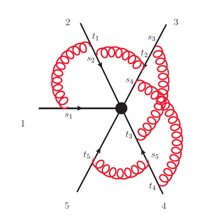
Figure 1: An example of a multiple gluon exchange diagram connecting five Wilson lines at five loops; it is part of the (1,2,3,3,1) web. The lines meet at a local effective vertex representing the hard interaction. For this diagram $\Theta_{D}\big{[}\left\{s_{k},t_{k}\right\}\big{]}\,=\,\theta(t_{1}>s_{2})\,\theta(s_{3}>t_{2}>s_{4})\,\theta(t_{4}>s_{5}>t_{3})$.

we consider each of the Wilson lines in turn according to the chosen order, moving along each line starting at the far end and reaching the origin; gluons are assigned the ordering with which they are encountered in this procedure. A given gluon $k$ is counted only once, as it is first encountered. With this assignment, we say that the $k$-th gluon is emitted from the Wilson line in the direction $\beta_{i(k)}$ at point $s_{k}$, and is absorbed by the Wilson line in the direction $\beta_{f(k)}$ at point $t_{k}$. Using the coordinate space Feynman gauge gluon propagator

$$D_{\mu\nu}^{ab}(x)\,=\,-\,\frac{\Gamma(1-\epsilon)}{4\,\pi^{2-\epsilon}}\,g_{\mu\nu}\,\delta^{ab}\,\left(-x^{2}+{\rm i}\varepsilon\right)^{-1+\epsilon}\,,$$ (21)

and expanding the Wilson line operators in eq. (5) in powers of the coupling, one easily finds that the most general $n$-gluon MGE Feynmam diagram $D$, contributing to eq. (20) at $n$ loops, can be written as

$${\cal F}^{(n)}\left(D\right) = \left(g^{2}\mu^{2\epsilon}\,\frac{\Gamma(1-\epsilon)}{4\pi^{2-\epsilon}}\right)^{n}\,\prod_{k=1}^{n}\beta_{i(k)}\cdot\beta_{f(k)}\,\int_{0}^{\infty}\prod_{k=1}^{n}ds_{k}\,dt_{k}\,\Theta_{D}\big{[}\left\{s_{k},t_{k}\right\}\big{]}$$

$$\!\!\!\!\!\!\!\!\!\!\!\prod_{k=1}^{n}\left[-\left(\beta_{i(k)}s_{k}-\beta_{f(k)}t_{k}\right)^{2}\right]^{-1+\epsilon}\exp\left[-\,{\rm i}m\sum_{k=1}^{n}\left(s_{k}\sqrt{\beta_{i(k)}^{2}-{\rm i}\varepsilon}+t_{k}\sqrt{\beta_{f(k)}^{2}-{\rm i}\varepsilon}\right)\right]\,.$$

Clearly the ordering of the attachments of the gluons on each Wilson line is essential: it is given by the function $\Theta_{D}\left[\left\{s_{k},t_{k}\right\}\right]$, which is a product of Heaviside functions assigned to each Wilson line, with $p-1$ independent $\theta$ functions on a line with $p$ gluon attachments.

Following Ref. Gardi:2013saa , we proceed by rescaling the Wilson line coordinates by defining

$$\sigma_{k}\,=\,s_{k}\sqrt{\beta_{i(k)}^{2}}\,,\qquad\tau_{k}\,=\,t_{k}\sqrt{\beta_{f(k)}^{2}}\,,$$ (23)

and furthermore we change variables by writing

$$\sigma_{k}\,=\,x_{k}\lambda_{k}\,,\qquad\tau_{k}\,=\,(1-x_{k})\lambda_{k}\,.$$ (24)

In this way, $\lambda_{k}$ is a measure of the overall distance of the $k$-th gluon from the origin, whereas $x_{k}$ is an ‘angular’ variable, measuring the degree of collinearity of the $k$-th gluon to either the emitting (as $x_{k}\to 1$) or the absorbing (as $x_{k}\to 0$) Wilson lines. In terms of these variables one finds

$${\cal F}^{(n)}\left(D\right) = \left(\frac{1}{2}\,g^{2}\mu^{2\epsilon}\,\frac{\Gamma(1-\epsilon)}{4\pi^{2-\epsilon}}\right)^{n}\,\times\,\int_{0}^{\infty}\prod_{k=1}^{n}d\lambda_{k}\,\lambda_{k}^{-1+2\epsilon}\,{\rm e}^{-{\rm i}(m-{\rm i}\varepsilon)\sum_{k=1}^{n}\lambda_{k}}$$

$$\times\,\,\int_{0}^{1}\prod_{k=1}^{n}dx_{k}\,\gamma_{k}\,\Big{[}-x_{k}^{2}-(1-x_{k})^{2}+\gamma_{k}\,x_{k}(1-x_{k})\Big{]}^{-1+\epsilon}\,\Theta_{D}\big{[}\left\{x_{k},\lambda_{k}\right\}\big{]}\,,$$

where $\gamma_{k}\equiv\gamma_{i(k),f(k)}$ was defined in eq. (3). Note that the distance variables $\lambda_{k}$ have been scaled out of the propagators. We keep using the symbol $\Theta_{D}$ for the product of Heaviside functions, although now they are expressed in terms of the new variables.

To proceed we now extract from the diagram the overall ultraviolet singularity arising from the region where all gluons are emitted and absorbed very close to the origin. In order to do so, we change variable again expressing the $\lambda_{k}$’s as

$$\lambda_{k}\,=\,\left(1-y_{k-1}\right)\,\prod_{p=k}^{n}y_{p}\,,$$ (26)

for $k=1,\ldots,n$, where we define $y_{0}=0$. Note that with this definition $\sum_{i=1}^{k}{\lambda_{i}}=\prod_{p=k}^{n}y_{p}$, and in particular the regulator in eq. (3.1), which involves the sum of all the $\lambda_{i}$, depends only on $y_{n}$. The Jacobian of this change of variables is given by $J=\prod_{k}y_{k}^{k-1}$, so, after performing the integral over $y_{n}$, we find

$${\cal F}^{(n)}\left(D\right) = \left(-\frac{1}{2}g^{2}\left(\frac{\mu^{2}}{m^{2}}\right)^{\epsilon}\,\frac{\Gamma(1-\epsilon)}{4\pi^{2-\epsilon}}\right)^{n}\,\Gamma(2n\epsilon)$$

$$\hskip 14.22636pt\times\,\,\int_{0}^{1}\prod_{k=1}^{n}dx_{k}\,\gamma_{k}\,\Big{[}x_{k}^{2}+(1-x_{k})^{2}-\gamma_{k}\,x_{k}(1-x_{k})\Big{]}^{-1+\epsilon}$$

$$\hskip 14.22636pt\times\,\,\int_{0}^{1}\prod_{k=1}^{n-1}dy_{k}\left(1-y_{k}\right)^{-1+2\epsilon}\,y_{k}^{-1+2k\epsilon}\,\,\,\Theta_{D}\big{[}\left\{x_{k},y_{k}\right\}\big{]}$$

$$= \kappa^{n}\,\,\Gamma(2n\epsilon)\,\int_{0}^{1}\prod_{k=1}^{n}\Big{[}dx_{k}\,\gamma_{k}\,P_{\epsilon}\left(x_{k},\gamma_{k}\right)\Big{]}\,\phi_{D}^{(n)}\left(x_{i};\epsilon\right)\,,$$

where we defined the coefficient

$$\kappa\,\equiv-\frac{1}{2}\,g^{2}\left(\frac{\mu^{2}}{m^{2}}\right)^{\epsilon}\,\frac{\Gamma(1-\epsilon)}{4\pi^{2-\epsilon}}\,,$$ (28)

as well as the function

$$P_{\epsilon}\left(x,\gamma\right)\,\equiv\,\left[x^{2}+(1-x)^{2}-x(1-x)\gamma)\right]^{-1+\epsilon}\,,$$ (29)

related to the gluon propagator, and the kernel

$$\phi_{D}^{(n)}\left(x_{i};\epsilon\right)\,=\,\int_{0}^{1}\prod_{k=1}^{n-1}dy_{k}\left(1-y_{k}\right)^{-1+2\epsilon}\,y_{k}^{-1+2k\epsilon}\,\,\Theta_{D}\big{[}\left\{x_{k},y_{k}\right\}\big{]}\,.$$ (30)

The analysis of Ref. Gardi:2013saa shows that $\phi_{D}^{(n)}\left(x_{i};\epsilon\right)$ has a Laurent expansion in $\epsilon$, $\phi_{D}^{(n)}=\sum_{k}\phi_{D}^{(n,k)}\epsilon^{k}$, where each term $\phi_{D}^{(n,k)}$ is a pure transcendental function of uniform weight $n-1+k$, containing logarithms and polylogarithms, as well as Heaviside functions depending on ratios of the variables $x_{i}$ or $1-x_{i}$.

3.2 Feynman integral for a MGE web

The next observation Gardi:2013saa is that all diagrams $D$ in a given web $W$ have a common integral structure of the form of eq. (3.1): assuming that in all diagrams $D\in W$ gluon $k$ is exchanged between the same pair of Wilson lines, such diagrams are only distinguished by the Heaviside functions $\Theta_{D}\big{[}\left\{x_{k},y_{k}\right\}\big{]}$ representing the order of gluon attachments to the Wilson lines, hence they only differ by their kernels $\phi_{D}^{(n)}\left(x_{i};\epsilon\right)$. Because a web $W$ is defined as a linear combination of the contributing diagrams $D\in W$, one deduces that the web as a whole takes a form similar to eq. (3.1). To see this in more detail, recall that, according to eq. (13), every web can contribute to different colour structures $c_{j}^{(L)}$ building up the anomalous dimension, $W^{(n)}=\sum_{j=1}^{r}{\cal F}_{W,j}^{(n)}\,{c_{j}^{(L)}}$, where the kinematic functions are specific linear combinations of the integrals corresponding to individual diagrams in the web,

$${\cal F}_{W,\,j}^{(n)}\left(\gamma_{ij},\epsilon\right)\,=\,\sum_{D\in W}Y_{D,j}^{-1}\,{\cal F}^{(n)}(D)\,,$$ (31)

and where the numerical coefficients $Y_{D,j}^{-1}$ are fixed by the web mixing matrix. One concludes that the contribution of web $W$ to the $j$-th colour structure is given by an integral similar to eq. (3.1),

$${\cal F}_{W,\,j}^{(n)}\left(\gamma_{ij},\epsilon\right)\,=\,\kappa^{n}\,\Gamma(2n\epsilon)\,\int_{0}^{1}\prod_{k=1}^{n}\Big{[}dx_{k}\,\gamma_{k}\,P_{\epsilon}\left(x_{k},\gamma_{k}\right)\Big{]}\,\phi_{W,\,j}^{(n)}\left(x_{i};\epsilon\right)\,,$$ (32)

with a web kernel given by

$$\phi^{(n)}_{W,\,j}\left(x_{i};\epsilon\right)\,=\,\sum_{D\in W}Y_{D,j}^{-1}\,\phi^{(n)}_{D}\left(x_{i};\epsilon\right)\,.$$ (33)

Before proceeding, it is useful to contrast non-Abelian MGEWs with their much simpler Abelian counterparts. According to the Abelian exponentiation theorem only connected graphs enter the exponent, so in particular Abelian MGEWs are not part of the exponent. Instead, they are reproduced by expanding the exponential involving a single exchange between each pair of Wilson lines. Because in the Abelian theory ordering is immaterial, one simply sums all diagrams with equal weights. This sum must yield a product of the relevant one-loop integrals. The result can readily be verified from eq. (3.1): indeed

$$\sum_{D\in W}{\cal F}^{(n)}\left(D\right) = \kappa^{n}\,\Gamma(2n\epsilon)\,\int_{0}^{1}\prod_{k=1}^{n}\Big{[}dx_{k}\,\gamma_{k}\,P_{\epsilon}\left(x_{k},\gamma_{k}\right)\Big{]}\,\sum_{D\in W}\phi_{D}^{(n)}\left(x_{i};\epsilon\right)$$ (34)

$$= \Big{(}\kappa\,\Gamma(2\epsilon)\Big{)}^{n}\,\,\int_{0}^{1}\prod_{k=1}^{n}\Big{[}dx_{k}\,\gamma_{k}\,P_{\epsilon}\left(x_{k},\gamma_{k}\right)\Big{]}\,,$$

where in the second line we used the fact that the sum of Heaviside functions for a MGEW gives unity, so that one can use

$$\sum_{D\in W}\phi_{D}^{(n)}\left(x_{i};\epsilon\right)\,=\,\int_{0}^{1}\prod_{k=1}^{n-1}dy_{k}\left(1-y_{k}\right)^{-1+2\epsilon}\,y_{k}^{-1+2k\epsilon}\,=\,\frac{\left(\Gamma(2\epsilon)\right)^{2}}{\Gamma(2n\epsilon)}\,.$$ (35)

As expected, eq. (34) is a product of one-loop integrals associated to the relevant cusp angles. The unweighted sum in eq. (35) is a constraint on the web kernels of any non-Abelian MGEW, providing a valuable check of explicit calculations in what follows.

3.3 Feynman integral for a MGE subtracted web

An important conclusion of the analysis in Ref. Gardi:2013saa is that the integration over the angular variables $x_{k}$ in eq. (32) is vastly simplified for subtracted webs. To this end, each web is expanded in powers of $\epsilon$, as

$$W^{(n)}\left(\gamma_{ij},\epsilon\right)\,=\,\alpha_{s}^{n}\sum_{k=-n}^{\infty}w^{(n,k)}\left(\gamma_{ij}\right)\,\epsilon^{k}\,,$$ (36)

and then it is combined with the commutators of the webs composed by its subdiagrams, according to the pattern forming the anomalous dimension in eq. (2.1). Then, in the notation of eq. (11), $\Gamma^{(n)}\,=\,-2n\,\sum_{i}\overline{w}^{(n,-1)}_{i}$. This step relies on the fact that the commutators build up the same colour factors and similar kinematic integrals as those of the web itself, eq. (32). The ${\cal O}(\alpha^{n},\epsilon^{-1})$ subtracted web can then be written as

$$\overline{w}^{(n,-1)}\left(\alpha_{k}\right)\,=\,\left(\frac{1}{4\pi}\right)^{n}\,\sum_{j=1}^{r}\,c_{j}^{(L)}\,F^{(n)}_{W,\,j}\big{(}\alpha_{k}\big{)}\,,$$ (37)

where we chose to express the kinematic dependence in terms of $\alpha_{k}\equiv\alpha_{i(k),f(k)}$, as defined in eq. (2), so that for each gluon $\gamma_{k}\,=-\,\alpha_{k}-1/\alpha_{k}$. Following Ref. Gardi:2013saa , we then define the functions of the $\alpha$ variables which arise from the gluon propagators as

$$p_{\epsilon}\left(x,\alpha\right)\,\equiv\,-\,\left(\alpha+\frac{1}{\alpha}\right)\,\Big{[}q(x,\alpha)\Big{]}^{-1+\epsilon}\,;\quad q\left(x,\alpha\right)\,\equiv\,x^{2}+(1-x)^{2}+\left(\alpha+\frac{1}{\alpha}\right)\,x(1-x)\,.$$ (38)

Upon expanding $p_{\epsilon}(x,\alpha)$ in powers of $\epsilon$ we get

$$p_{\epsilon}\left(x,\alpha\right)\,=\,p_{0}\left(x,\alpha\right)\,\sum_{n=0}^{\infty}\frac{\epsilon^{n}}{n!}\Big{[}\log q\left(x,\alpha\right)\Big{]}^{n}\,,$$ (39)

where

$$p_{0}\left(x,\alpha\right)\,=\,-\,\left(\alpha+\frac{1}{\alpha}\right)\,\frac{1}{q(x,\alpha)}\,=\,r(\alpha)\left[\frac{1}{x-\frac{1}{1-\alpha}}-\frac{1}{x+\frac{\alpha}{1-\alpha}}\right]\,,$$ (40)

and where the rational function $r(\alpha)$ is given by

$$r(\alpha)\,=\,\frac{1+\alpha^{2}}{1-\alpha^{2}}\,.$$ (41)

Using these notations, the subtracted web kinematic function $F^{(n)}_{W,\,j}$ can be written as

$$F^{(n)}_{W,\,j}\big{(}\alpha_{i}\big{)} = \int_{0}^{1}\left[\,\prod_{k=1}^{n}dx_{k}\,p_{0}(x_{k},\alpha_{k})\right]\,{\cal G}^{(n)}_{W,\,j}\Big{(}x_{i},q(x_{i},\alpha_{i})\Big{)}\,$$ (42)

$$= \,\left(\prod_{k=1}^{n}r(\alpha_{k})\right)\int_{0}^{1}\left[\prod_{k=1}^{n}dx_{k}\left(\frac{1}{x_{k}-\frac{1}{1-\alpha_{k}}}-\frac{1}{x_{k}+\frac{\alpha_{k}}{1-\alpha_{k}}}\right)\right]\,{\cal G}^{(n)}_{W,\,j}\Big{(}x_{i},q(x_{i},\alpha_{i})\Big{)}\,$$

$$\equiv \,\left(\prod_{k=1}^{n}r(\alpha_{k})\right)G^{(n)}_{W,\,j}\big{(}\alpha_{i}\big{)}\,,$$

where in the first line we introduce the subtracted web kernel ${\cal G}^{(n)}_{W,\,j}$. This function contains the finite term of the web kernel $\phi_{W,\,j}^{(n)}\left(x_{i};\epsilon\right)$, along with related terms from the commutators of the relevant subdiagrams; additional contributions occur due to (multiple) poles of $\phi_{W,\,j}^{(n)}\left(x_{i};\epsilon\right)$, related to subdivergences, which are multiplied by appropriate powers of $\log q\left(x,\alpha\right)$ from the expansion in eq. (39). In the second expression in eq. (42) we used the partial fraction form of $p_{0}$ introduced in eq. (40), which is the convenient form for performing the $x_{k}$ integrals. This also fixes the rational function associated with the web, which is simply a factor of $r(\alpha_{k})$ for each gluon exchange. In the final expression in eq. (42) all the $x_{k}$ integrals are done, defining the function $G^{(n)}_{W,\,j}\big{(}\alpha_{i}\big{)}$.

As discussed in Ref. Gardi:2013saa , remarkable simplifications occur at the level of eq. (42). These can most easily be described through the properties of the subtracted web kernel ${\cal G}^{(n)}_{W,\,j}$: this function depends on its arguments only through powers of the logarithms, $\ln(x_{k})$, $\ln(1-x_{k})$ and $\ln q(x_{k},\alpha_{k})$, and through Heaviside functions involving ratios of the variables $x_{k}$. The integrals in the second line of eq. (42) are of a $d\log$ form. Thus, the resulting function $G^{(n)}_{W,\,j}\big{(}\alpha_{i}\big{)}$ is a pure function of transcendental weight $2n-1$. Subtracted multi-particle webs thus share the properties of two-parton webs described in Ref. Henn:2013wfa . It should be stressed, however, that the route by one which calculates multiparton webs is substantially different, due to the combinatorics associated with the non-trivial colour structure, and to the presence of subdivergences.

We emphasise that the absence of polylogarithms in ${\cal G}^{(n)}_{W,\,j}$ is rather surprising: recall that polylogarithms of weight $n-1$ do occur in the ${\cal O}(\epsilon^{0})$ term of the non-subtracted web kernel $\phi_{W,\,j}^{(n)}\left(x_{i};\epsilon\right)$. Ref. Gardi:2013saa argued that these polylog cancellations (and the related analytic properties of $G^{(n)}_{W,\,j}\big{(}\alpha_{i}\big{)}$, which we describe below) are linked with the restoration of crossing symmetry. The latter is lost at the level of non-subtracted webs, due the action of the infrared regulator in the presence of ultraviolet subdivergences, but it is recovered for subtracted webs.

The most important consequence of the purely logarithmic nature of the subtracted web kernel is that the resulting integrated function, $G^{(n)}_{W,\,j}\big{(}\alpha_{i}\big{)}$, is a sum of products of polylogarithms, each depending on a single $\alpha_{k}$ variable. Furthermore, these polylogarithms are very specific; their symbol alphabet is restricted to $\alpha_{k}$ and $1-\alpha_{k}^{2}$. The goal of the next section is to fully characterize these functions and obtain an explicit basis for them.

It should be stressed that the properties just described have been conjectured to be general, but they have not been proven. Specifically, all explicit calculations in Ref. Gardi:2013saa were of webs whose subtracted kernel is free of Heaviside functions, in which case the relation between the purely logarithmic nature of the kernel and the factorization property is obvious. Such a relation is less obvious when Heaviside functions occur in ${\cal G}^{(n)}_{W,\,j}$. The number of Heaviside functions appearing in a given subtracted web kernel depends on the level of entanglement of the web: webs spanning the maximal number, $n+1$, of Wilson lines at $n$ loops are not entangled (so there is no Heaviside function after performing the $y_{k}$ integrals in eq. (30)) while those connecting fewer Wilson lines are entangled by up to $n-1$ Heaviside functions. A central goal of the present paper is to verify that the factorization property does indeed hold even for entangled webs.

4 A basis of functions for MGEWs

4.1 Constructing a basis

One of the conclusions of Ref. Gardi:2013saa is that the subtracted webs (1,2,2,1) and (1,1,1,3), connecting the maximum possible number of Wilson lines at three loops, can be written in terms of the simple set of integrals

$$R_{0}(\alpha) = \frac{1}{r(\alpha)}\int_{0}^{1}dx\,p_{0}(x,\alpha)\,,$$

$$\Sigma_{2}(\alpha) = \frac{1}{2\,r(\alpha)}\int_{0}^{1}dx\,p_{0}(x,\alpha)\ln^{2}\bigg{(}\frac{x}{1-x}\bigg{)}\,,$$

$$U_{1}(\alpha) = \frac{1}{r(\alpha)}\int_{0}^{1}dx\,p_{0}(x,\alpha)\ln\bigg{(}\frac{q(x,\alpha)}{x^{2}}\bigg{)}\,,$$ (43)

$$U_{2}(\alpha) = \frac{1}{4\,r(\alpha)}\int_{0}^{1}dx\,p_{0}(x,\alpha)\ln^{2}\bigg{(}\frac{q(x,\alpha)}{x^{2}}\bigg{)}\,.$$

These integrals have an integrand consisting only of logarithms, depend upon only a single cusp angle, and individually satisfy the alphabet constraints outlined above. It is natural to ask whether one may construct a basis for all MGEWs, given the requirements of the alphabet and factorization conjectures, and the limited range of elements entering the subtracted web kernel in eq. (42), namely

$$\ln\frac{q(x,\alpha)}{x^{2}}\,=\,\ln\left(\frac{1}{x}+\alpha-1\right)+\ln\left(\frac{1}{x}+\frac{1}{\alpha}-1\right)\,.$$ (44)

and $\ln\Big{(}\frac{x}{1-x}\Big{)}$. A first attempt could be to consider the set of functions

$$M_{k,m}(\alpha)\,=\,\frac{1}{r(\alpha)}\int_{0}^{1}dx\,\,p_{0}(x,\alpha)\,\ln^{k}\bigg{(}\frac{q(x,\alpha)}{x^{2}}\bigg{)}\ln^{2m}\bigg{(}\frac{x}{1-x}\bigg{)}\,,$$ (45)

with $k$ and $m$ non-negative integers (note that $q(x,\alpha)$ is symmetric under $x\to 1-x$, and odd powers of $\ln\Big{(}\frac{x}{1-x}\Big{)}$ can be eliminated in terms of ones with even powers). The functions in eq. (45) have uniform weight $2m+k+1$, and they satisfy the alphabet conjecture. In terms of these functions one finds

$$\begin{split}R_{0}(\alpha)&=M_{0,0}(\alpha)\,,\quad\quad U_{1}(\alpha)=M_{1,0}(\alpha)\,,\\ \Sigma_{2}(\alpha)&=\frac{1}{2}M_{0,1}(\alpha)\,,\quad\,\,U_{2}(\alpha)=\frac{1}{4}M_{2,0}(\alpha)\,.\end{split}$$ (46)

At least through three loops, the basis of eq. (45) is sufficient to describe MGEWs that connect the maximum number of Wilson lines at a given loop order. We now wish to check whether more entangled webs, which connect fewer lines, and thus may have leftover Heaviside functions in their subtracted web kernel ${\cal G}_{W}$, will belong to the span of this basis. To do this, we shall first consider the (2,2) web at two loops, and then the (3,3), (1,2,3), and (2,2,2) subtracted webs at three loops. The relevant combination of effective vertices are, respectively: $V^{(1)}_{2}V^{(2)}_{2}$, $V^{(1)}_{3}V^{(2)}_{3}$, $V^{(1)}_{1}V^{(2)}_{2}V^{(3)}_{3}$ and $V^{(1)}_{2}V^{(2)}_{2}V^{(3)}_{2}$.

Let us begin by considering the simplest example, the two-loop, two-line 2-2 web, which is of course well-known Korchemsky:1987wg ; Kidonakis:2009ev . This web contains two diagrams: the ladder ($II$) and the crossed (${\rm X}$) one. It is immediately evident, however, according to the definition of webs for the colour-singlet case Gatheral:1983cz ; Frenkel:1984pz , that only the kinematic integral of the latter, shown in Fig. 2, contributes. The web therefore evaluates to

$$W_{(2,2)}^{(2)}\,=\,\Big{[}C(X)-C(II)\Big{]}{\cal F}(X)\,=\,\frac{1}{2}[T_{1}^{a},T_{1}^{b}]\,[T_{2}^{b},T_{2}^{a}]\,{\cal F}(X)\,=\,\frac{N_{c}}{2}T_{1}\cdot T_{2}\,{\cal F}(X)\,.$$ (47)

A derivation of this result using the effective vertex formalism was given in Section 3 of Ref. Gardi:2013ita , where it was shown that the only contribution arises from a double-emission vertex $V_{2}$ on each of the two Wilson lines, each vertex having a connected colour structure given by eq. (14).

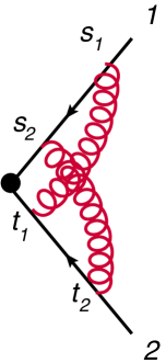
Figure 2: The two-loop crossed graph connecting two Wilson lines, and the corresponding effective vertex graph containing a double emission vertex $V_{2}$ on each of the two lines.

We now proceed to consider the integral ${\cal F}(X)$. Specifically we will be interested in the simple pole of this function,

$${\cal F}(X)\,=\,\left(\frac{\alpha_{s}}{4\pi}\right)^{2}\left[\frac{1}{\epsilon}\,F^{(2)}_{(2,2)}(\alpha)+{\cal O}(\epsilon^{0})\,\right]\,,$$ (48)

which depends on a single kinematic variable, $\alpha_{12}\equiv\alpha$. In the notation of eq. (3.1), one has four semi-infinite parameter integrals, two over $s_{1}$ and $s_{2}$ along line 1, and two over $t_{1}$ and $t_{2}$ along line 2, with the restrictions $\Theta_{X}=\theta(s_{1}-s_{2})\,\theta(t_{2}-t_{1})$. Following the steps leading to eq. (42), we find

$$F^{(2)}_{(2,2)}(\alpha)\,=\,\int_{0}^{1}dx_{1}\int_{0}^{1}dx_{2}\,p_{0}(x_{1},\alpha)\,p_{0}(x_{2},\alpha)\,{\cal G}^{(2)}_{(2,2)}(x_{1},x_{2})\,,$$ (49)

with the kernel

$${\cal G}^{(2)}_{(2,2)}(x_{1},x_{2})\,=\,\theta(x_{1}-x_{2})\ln\bigg{(}\frac{x_{1}}{1-x_{1}}\frac{1-x_{2}}{x_{2}}\bigg{)}\,.$$ (50)

Using $p_{0}(1-x,\alpha)=p_{0}(x,\alpha)$, we can write the kinematic factor in eq. (49) as

$$F^{(2)}_{(2,2)}(\alpha)\,=\,2\int_{0}^{1}dx_{1}\,p_{0}(x_{1},\alpha)\ln\bigg{(}\frac{x_{1}}{1-x_{1}}\bigg{)}\int_{0}^{1}dx_{2}\,p_{0}(x_{2},\alpha)\,\theta(x_{1}-x_{2})\,.$$ (51)

The second integral in eq. (51) does not yield an expression of the form of eq. (45), so we shall be forced to extend our basis. Let us proceed as follows. First we define

$$\ln\tilde{q}(x,\alpha)\,\equiv\,\frac{1}{r(\alpha)}\int_{0}^{1}dy\,p_{0}(y,\alpha)\theta(x-y)\,=\ln\left(\frac{1}{x}+\alpha-1\right)-\ln\left(\frac{1}{x}+\frac{1}{\alpha}-1\right)\,.$$ (52)

We may then extend our basis by defining the set of functions

$$M_{k,l,n}(\alpha)\,=\,\frac{1}{r(\alpha)}\int_{0}^{1}dx\,p_{0}(x,\alpha)\ln^{k}\bigg{(}\frac{q(x,\alpha)}{x^{2}}\bigg{)}\ln^{l}\bigg{(}\frac{x}{1-x}\bigg{)}\ln^{n}\tilde{q}(x,\alpha)\,.$$ (53)

These functions have uniform weight ${\rm w}=k+l+n+1$, and we will see below that $M_{k,l,n}(\alpha)$ still gives rise to the required alphabet composed of $\alpha$ and $\eta=\alpha/(1-\alpha^{2})$. Clearly, these functions are consistent with our constraints. Note also that $\ln\tilde{q}(x,\alpha)$ is a natural addition to the previous basis: as shown in eq. (52), it is precisely the difference of the same two logarithms whose sum is given by the factor in eq. (44). Notice also that $\ln\tilde{q}(x,\alpha)$ is odd under $\alpha\to 1/\alpha$, while the full result for every web must be even, because of the relation between $\alpha$ and $\gamma$. Therefore if this logarithm appears raised to an odd power, the symmetry in the corresponding contribution will have to be restored by some other factor in the result, for example a factor of $r(\alpha)$, or multiplication by another function of the basis also odd under the same transformation.

We can now revisit eq. (51), and express the result for the (2,2) web in terms of the basis in eq. (53)), as

$$\overline{w}^{(2)}_{(2,2)}\,=\,\left(\frac{1}{4\pi}\right)^{2}\frac{N_{c}}{2}\,\,T_{1}\cdot T_{2}\,\,F^{(2)}_{(2,2)}(\alpha)\,,\qquad\quad F^{(2)}_{(2,2)}(\alpha)\,=\,2\,r^{2}(\alpha)\,M_{0,1,1}(\alpha)\,.$$ (54)

By using the explicit expression for the function $M_{0,1,1}(\alpha)$ given in Appendix A, we see that this result agrees with the calculation reported in Korchemsky:1987wg ; Kidonakis:2009ev .

Having fixed the basis, we can readily express all previously computed subtracted webs in terms of the first few basis functions. To begin with, the functions in eq. (4.1) can be expressed in terms of eq. (53) as

$$\begin{split}R_{0}(\alpha)&=M_{0,0,0}(\alpha)\,,\quad\,\,\,\,\,U_{1}(\alpha)=M_{1,0,0}(\alpha)\,,\\ \Sigma_{2}(\alpha)&=\frac{1}{2}M_{0,2,0}(\alpha)\,,\quad U_{2}(\alpha)\,=\,\frac{1}{4}M_{2,0,0}(\alpha)\,.\end{split}$$ (55)

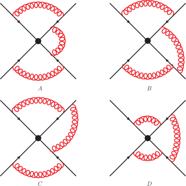
Figure 3: The (1,2,2,1) web, connecting four Wilson lines at three loops.

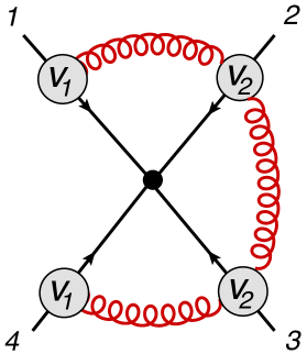
Figure 4: The (1,2,2,1) web in the effective vertex formalism.

Further, the (1,2,1) subtracted web computed in Ferroglia:2009ep ; Ferroglia:2009ii ; Mitov:2010xw ; Chien:2011wz ; Gardi:2013saa can be written as

$$\overline{w}_{121}^{(2,-1)} = -\,{\rm i}\,f^{abc}T_{i}^{a}T_{j}^{b}T_{k}^{c}\,\left(\frac{1}{4\pi}\right)^{2}\,\frac{1}{2}\,r(\alpha_{ij})\,r(\alpha_{jk})\,$$

$$\hskip 28.45274pt\times\,\Big{(}M_{0,0,0}(\alpha_{ij})M_{1,0,0}(\alpha_{jk})-M_{0,0,0}(\alpha_{jk})M_{1,0,0}(\alpha_{ij})\Big{)}\,,$$

Next, the results of the (1,2,2,1) and (1,1,1,3) subtracted webs, computed in Ref. Gardi:2013saa , can be expressed in the new basis as follows. For the (1,2,2,1) web of Fig. 3, whose colour structure in the effective vertex formalism is shown in Fig. 4, one finds

$$\overline{w}^{(3)}_{(1,2,2,1)}\left(\alpha_{12},\alpha_{23},\alpha_{34}\right) = -\frac{1}{6}\,f_{abe}f^{e}_{\phantom{e}cd}T_{1}^{a}T_{2}^{b}T_{3}^{c}T_{4}^{d}\,\,\left(\frac{1}{4\pi}\right)^{3}r(\alpha_{12})\,r(\alpha_{23})\,r(\alpha_{34})$$ (57)

$$\hskip 56.9055pt\times\,G_{(1,2,2,1)}\left(\alpha_{12},\alpha_{23},\alpha_{34}\right)\,,$$

where

$$G_{(1,2,2,1)}\left(\alpha_{12},\alpha_{23},\alpha_{34}\right)\,=\,-\,\frac{1}{2}\,M_{2,0,0}(\alpha_{12})M_{0,0,0}(\alpha_{23})M_{0,0,0}(\alpha_{34})$$ (58)

$$-\,\frac{1}{2}\,M_{2,0,0}(\alpha_{34})M_{0,0,0}(\alpha_{12})M_{0,0,0}(\alpha_{23})+M_{2,0,0}(\alpha_{23})M_{0,0,0}(\alpha_{12})M_{0,0,0}(\alpha_{34})$$

$$-\,M_{0,0,0}(\alpha_{12})M_{1,0,0}(\alpha_{23})M_{1,0,0}(\alpha_{34})-M_{0,0,0}(\alpha_{34})M_{1,0,0}(\alpha_{12})M_{1,0,0}(\alpha_{23})$$

$$+\,2\,M_{0,0,0}(\alpha_{23})M_{1,0,0}(\alpha_{12})M_{1,0,0}(\alpha_{34})-4\,M_{0,2,0}(\alpha_{23})M_{0,0,0}(\alpha_{12})M_{0,0,0}(\alpha_{34})\,.$$

For the (1,1,1,3) web, whose colour structure is depicted in figure 5, one finds

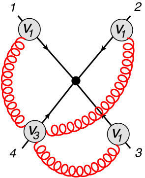
Figure 5: Effective vertex diagram for the (1,1,1,3) web.

$$\overline{w}^{(3)}_{(1,1,1,3)}\left(\alpha_{14},\alpha_{24},\alpha_{34}\right) = -\frac{1}{6}\,T_{1}^{a}T_{2}^{b}T_{3}^{c}T_{4}^{d}\,\left(\frac{1}{4\pi}\right)^{3}r(\alpha_{14})\,r(\alpha_{24})\,r(\alpha_{34})$$ (59)

$$\times\,\Big{[}f_{ade}f^{e}_{\phantom{e}bc}\,G_{(1,1,1,3)}\left(\alpha_{14},\alpha_{24},\alpha_{34}\right)+f_{ace}f^{e}_{\phantom{e}bd}\,G_{(1,1,1,3)}\left(\alpha_{24},\alpha_{14},\alpha_{34}\right)\Big{]}\,,$$

where

$$G_{(1,1,1,3)}\left(\alpha_{14},\alpha_{24},\alpha_{34}\right)\,=\,\frac{1}{2}\,M_{2,0,0}(\alpha_{14})M_{0,0,0}(\alpha_{24})M_{0,0,0}(\alpha_{34})$$ (60)

$$+\,\frac{1}{2}\,M_{2,0,0}(\alpha_{34})M_{0,0,0}(\alpha_{14})M_{0,0,0}(\alpha_{24})-\,M_{2,0,0}(\alpha_{24})M_{0,0,0}(\alpha_{14})M_{0,0,0}(\alpha_{34})$$

$$+\,M_{0,0,0}(\alpha_{14})M_{1,0,0}(\alpha_{24})M_{1,0,0}(\alpha_{34})+\,M_{0,0,0}(\alpha_{34})M_{1,0,0}(\alpha_{14})M_{1,0,0}(\alpha_{24})$$

$$-\,2\,M_{0,0,0}(\alpha_{24})M_{1,0,0}(\alpha_{14})M_{1,0,0}(\alpha_{34})\,.$$

We note that, while the weight of $G$ is ${\rm w}=2n-1$, these webs span $n+1$ Wilson lines at order $n$, involving $n$ individual gluons, each depending on a separate $\alpha_{ij}$. Thus the weight w is partitioned so that each term involves a function of ${\rm w}\geq 1$ for each of the $n$ gluons. Consequently, we only encounter functions up to weight ${\rm w}=n$. To explore the validity of the basis beyond weight 3 we need to either consider more entangled webs spanning fewer lines, where fewer, but higher weight functions enter, or explore higher loop corrections. In the following we will do both.

As a first step, we need to generate the basis functions up to weight five (this will be sufficient for the calculations we present in this paper). Before doing so, however, we must note that not all functions $M_{k,l,n}$ are independent, and we must discuss the relevant degeneracies. As an example, in the $n=0$ case one finds that

$$M_{k,2\lambda+1,0}(\alpha)\,=\,-\,\sum_{r=1}^{k}\left(\begin{array}[]{c}k\\ r\end{array}\right)2^{r-1}\,M_{k-r,2\lambda+1+r,0}(\alpha)\,,$$ (61)

so, for $n=0$, we can recursively express all the functions with odd values of $l$, in terms of those with even values of $l$. Similarly, we can find relations in the general case $n\neq 0$, by considering the symmetry under $x\leftrightarrow 1-x$. One verifies that

$$M_{k,l,n}(\alpha) = \frac{1}{r(\alpha)}\int_{0}^{1}dx\,p_{0}(x,\alpha)\,(-1)^{l+n}\left[\log\left(\frac{q(x,\alpha)}{x^{2}}\right)+2\log\left(\frac{x}{1-x}\right)\right]^{k}$$ (62)

$$\hskip 56.9055pt\times\,\left[\log\left(\frac{x}{1-x}\right)\right]^{l}\Big{[}\log(\tilde{q}(x,\alpha))-2\log(\alpha)\Big{]}^{n}\,.$$

By expanding the integrand in eq. (62) we obtain then the general relation

$$M_{k,l,n}(\alpha)\,=\,(-1)^{l+n}\sum_{r=0}^{k}\sum_{s=0}^{n}\left(\begin{array}[]{c}k\\ r\end{array}\right)\left(\begin{array}[]{c}n\\ s\end{array}\right)2^{s+r}(-1)^{s}\log^{s}(\alpha)\,M_{k-r,l+r,n-s}(\alpha)\,.$$ (63)

Once again, we can express $M_{k,l,n}$, with $l+n$ odd, in terms of the basis functions with $l+n$ even, and lower weights. Using these relations it is easy to derive the set of independent functions up to any desired weight. For example, at weight two, we have the relation

$$M_{0,0,1}(\alpha)\,=\,\frac{1}{2}M_{0,0,0}^{2}(\alpha)\,,$$ (64)

and at weight three we find

$$M_{1,1,0}(\alpha) = -\,M_{0,2,0}(\alpha)\,,$$

$$M_{1,0,1}(\alpha) = -\,M_{0,1,1}(\alpha)+\frac{1}{2}\,M_{0,0,0}(\alpha)M_{1,0,0}(\alpha)\,.$$ (65)

Using these relations to eliminate redundant entries, we give the basis functions up to weight ${\rm w}=5$ in Table 1. The table presents the symbol of each function, while explicit expressions in terms of classical and harmonic polylogarithms Remiddi:1999ew are given in Appendix A. All functions have the required symbol alphabet; consequently, they can all be expressed in terms of harmonic polylogarithms with entries $0$ and $1$.

$M_{k,l,n}(\alpha)$
w	Name	Symbol
1	$M_{0,0,0}$	$2\,(\otimes\alpha)$
2	$M_{1,0,0}$	$-4\,\alpha\otimes\eta$
3	$M_{0,0,2}$	$16\,\alpha\otimes\alpha\otimes\alpha$
	$M_{0,1,1}$	$-4\,\alpha\otimes\eta\otimes\alpha$
	$M_{0,2,0}$	$4\,\alpha\otimes\alpha\otimes\alpha$
	$M_{2,0,0}$	$16\,\alpha\otimes\eta\otimes\eta$
4	$M_{1,0,2}$	$-32\,\alpha\otimes\alpha\otimes\alpha\otimes\eta$
	$M_{1,1,1}$	$-16\,\alpha\otimes\alpha\otimes\alpha\otimes\alpha+8\,\alpha\otimes\eta\otimes\alpha\otimes\eta+8\,\alpha\otimes\eta\otimes\eta\otimes\alpha$
	$M_{1,2,0}$	$-8\,\alpha\otimes\alpha\otimes\alpha\otimes\eta-8\,\alpha\otimes\eta\otimes\alpha\otimes\alpha$
	$M_{3,0,0}$	$-96\,\alpha\otimes\eta\otimes\eta\otimes\eta$
5	$M_{0,0,4}$	$768\,\alpha\otimes\alpha\otimes\alpha\otimes\alpha\otimes\alpha$
	$M_{0,1,3}$	$-96\,\alpha\otimes\alpha\otimes\alpha\otimes\eta\otimes\alpha-96\,\alpha\otimes\alpha\otimes\eta\otimes\alpha\otimes\alpha-96\,\alpha\otimes\eta\otimes\alpha\otimes\alpha\otimes\alpha$
	$M_{0,2,2}$	$96\,\alpha\otimes\alpha\otimes\alpha\otimes\alpha\otimes\alpha+32\,\alpha\otimes\eta\otimes\alpha\otimes\eta\otimes\alpha$
	$M_{0,3,1}$	$-24\,\alpha\otimes\alpha\otimes\alpha\otimes\eta\otimes\alpha-24\,\alpha\otimes\eta\otimes\alpha\otimes\alpha\otimes\alpha$
	$M_{0,4,0}$	$48\,\alpha\otimes\alpha\otimes\alpha\otimes\alpha\otimes\alpha$
	$M_{2,0,2}$	$128\,\alpha\otimes\alpha\otimes\alpha\otimes\eta\otimes\eta$
	$M_{2,1,1}$	$64\,\alpha\otimes\alpha\otimes\alpha\otimes\alpha\otimes\eta+32\,\alpha\otimes\alpha\otimes\eta\otimes\alpha\otimes\alpha+32\,\alpha\otimes\eta\otimes\alpha\otimes\alpha\otimes\alpha$
		$-32\,\alpha\otimes\eta\otimes\alpha\otimes\eta\otimes\eta-32\,\alpha\otimes\eta\otimes\eta\otimes\alpha\otimes\eta-32\,\alpha\otimes\eta\otimes\eta\otimes\eta\otimes\alpha$
	$M_{2,2,0}$	$32\,\alpha\otimes\alpha\otimes\alpha\otimes\alpha\otimes\alpha+32\,\alpha\otimes\alpha\otimes\alpha\otimes\eta\otimes\eta+32\,\alpha\otimes\eta\otimes\alpha\otimes\alpha\otimes\eta$
		$+32\,\alpha\otimes\eta\otimes\eta\otimes\alpha\otimes\alpha$
	$M_{4,0,0}$	$768\,\alpha\otimes\eta\otimes\eta\otimes\eta\otimes\eta$

Table 1: Symbols of all the linearly independent functions of the MGEW basis of eq. (53), up to weight ${\rm w}=5$. We use the shorthand notation $\eta=\alpha/(1-\alpha^{2})$.

A crucial question at this point is whether further extensions of our proposed basis will be required at higher orders, when more entangled webs are present. In the following, we present several examples of webs at three and four loops, providing evidence that the basis of functions in eq. (53) is indeed sufficient. We begin by looking at the most entangled three-loop web, the (3,3) web involving only two Wilson lines.

4.2 Testing the basis: a three-loop, two-line web

In the colour singlet channel, the (3,3) web $W_{(3,3)}$ contributes to the three-loop cusp anomalous dimension, and it could easily be computed, for example, with the techniques of Ref. Henn:2013wfa . For open Wilson lines, the only minor complication is that two independent colour structures arise, while of course the relevant kinematic integrals are the same. The diagrams contributing to $W_{(3,3)}$ are displayed in Fig. 6, and are denoted by $(a)$ and $(b)$ respectively.

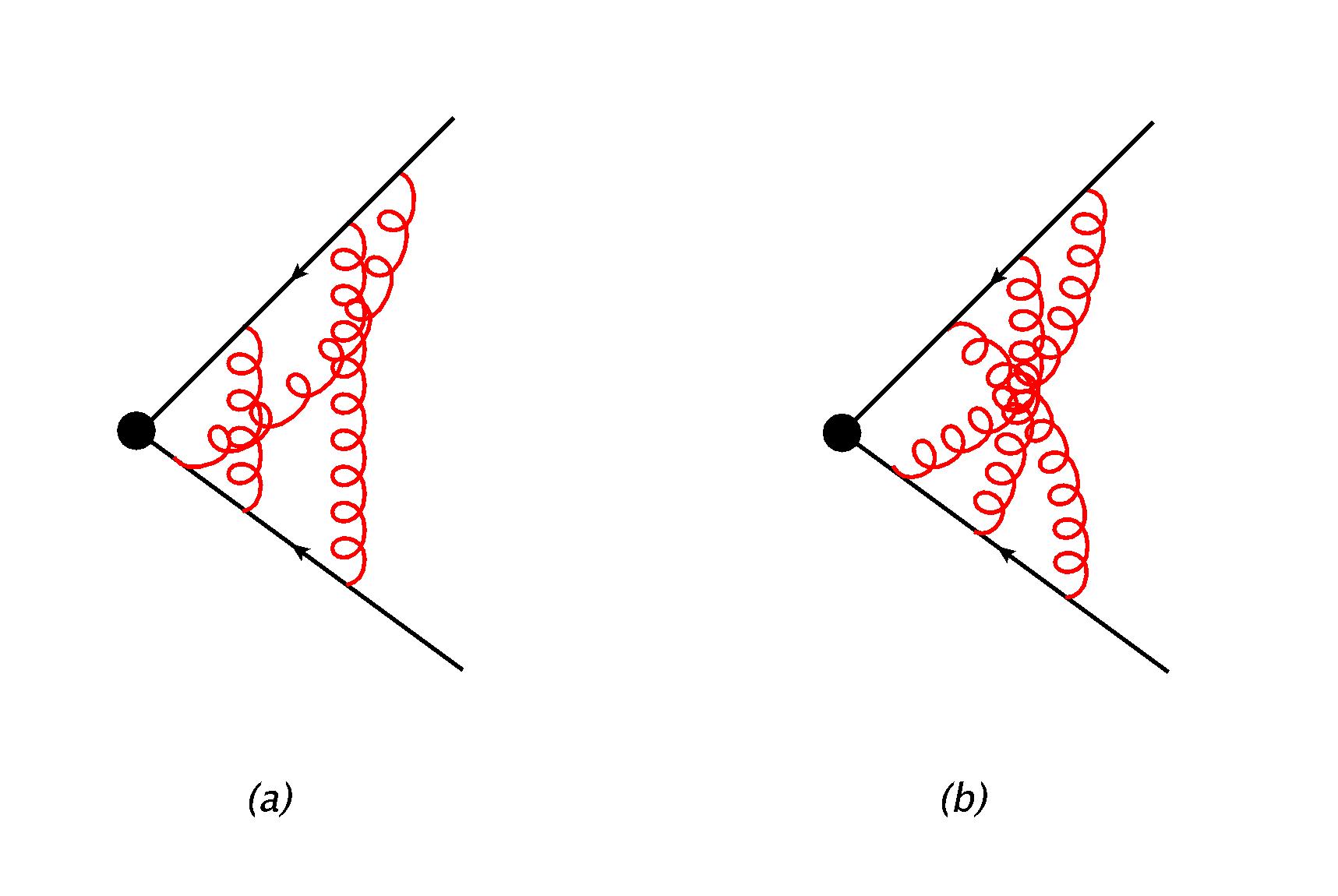
Figure 6: The two diagrams contributing to the (3,3) web at the three loop order. Diagram (a) has a twin under the symmetry swapping the two Wilson lines; its kinematic integral yields the same function as (a).

Using the procedure outlined in Sec. 3, it is straightforward to evaluate the contributions of the two diagrams to the web. Since these diagrams are irreducible, they each have just a single ultraviolet pole, and we define

$${\cal F}(a)\,=\,\left(\frac{\alpha_{s}}{4\pi}\right)^{3}\left[\frac{1}{\epsilon}\,F^{(3)}_{(3,3)}(a)+{\cal O}(\epsilon^{0})\,\right]\,,\quad{\cal F}(b)\,=\,\left(\frac{\alpha_{s}}{4\pi}\right)^{3}\left[\frac{1}{\epsilon}\,F^{(3)}_{(3,3)}(b)+{\cal O}(\epsilon^{0})\,\right]\,.$$ (66)

In the absence of subdivergences (in the colour singlet case, each diagram separately is a ‘web’ in the sense of Refs. Gatheral:1983cz ; Frenkel:1984pz ), no subtractions are needed. The entangled nature of the diagrams, which leads to the absence of subdivergences, also implies, however, that their contributions to the web kernel involve two Heaviside functions, as we shall see explicitly below.

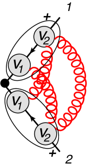
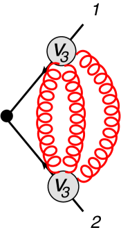
Figure 7: The elements of the (3,3) web in the effective vertex formalism. The diagram on the left hand side, where each Wilson line features a (symmetrized) pair of $V_{2}$ and $V_{1}$ vertices, can be obtained from the (1,2,2,1) web of figure 4 upon taking collinear limits, as explained in the text.

For open Wilson lines (that is to say, when the hard interaction vertex is not a colour singlet), one finds that the (3,3) web involves two independent colour structures. Working in the effective colour vertex basis, the result can be written as

$$\overline{w}^{(3)}_{(3,3)}(\alpha) = \left(\frac{1}{4\pi}\right)^{3}\,\frac{1}{4}\,\bigg{[}-f_{abe}\,f^{e}_{\phantom{e}cd}\Big{\{}T_{i}^{a},T_{i}^{c}\Big{\}}\Big{\{}T_{j}^{b},T_{j}^{d}\Big{\}}\,F^{(3)}_{(V_{1}V_{2})_{+}(V_{1}V_{2})_{+}}(\alpha)$$ (67)

$$\hskip 85.35826pt+\,{N_{c}^{2}}\,T_{i}\cdot T_{j}\,F^{(3)}_{V_{3}V_{3}}(\alpha)\bigg{]}\,,$$

where the first term involves the symmetric combination of a single emission vertex and a double emission vertex on each line, while the second term has one triple emission vertex per line. These two colour structures are depicted in Fig. 7. The linear combinations of kinematic integrals corresponding to each colour structure can be easily computed from the corresponding web mixing matrix Gardi:2013ita , and one finds

$$\begin{split}F^{(3)}_{(V_{1}V_{2})_{+}(V_{1}V_{2})_{+}}(\alpha)&=2\,F_{(3,3),a}^{(3)}(\alpha)+F_{(3,3),b}^{(3)}(\alpha)\,,\\ F^{(3)}_{V_{3}V_{3}}(\alpha)&=F_{(3,3),a}^{(3)}(\alpha)+\frac{3}{2}F_{(3,3),b}^{(3)}(\alpha)\,,\end{split}$$ (68)

where $F^{(3)}_{(3,3),j}(\alpha)$ with $j=a,b$ denotes the contributions of the two diagrams in Fig. 6. Following the steps described in Sec. 3, we get

$$F^{(3)}_{(3,3),j}(\alpha)\,=\,\int_{0}^{1}dx\int_{0}^{1}dy\int_{0}^{1}dz\,p_{0}(x,\alpha)\,p_{0}(y,\alpha)\,p_{0}(z,\alpha)\,{\cal G}^{(3)}_{(3,3),j}(x,y,z)$$ (69)

with the kernels

$$\mathcal{G}_{(3,3),\,a}^{(3)}\left(x,y,z\right) = -\frac{4}{3}\ln^{2}\bigg{(}\frac{x}{1-x}\frac{1-z}{z}\bigg{)}\,\theta(z-x)\,\theta(y-z)\,,$$

$$\mathcal{G}_{(3,3),\,b}^{(3)}\left(x,y,z\right) = -\frac{4}{3}\ln\bigg{(}\frac{x}{1-x}\frac{1-y}{y}\bigg{)}\ln\bigg{(}\frac{y}{1-y}\frac{1-z}{z}\bigg{)}\,\theta(y-x)\,\theta(z-y)\,.$$ (70)

Using eqs. (69) and (4.2) with the combination $F^{(3)}_{(V_{1}V_{2})_{+}(V_{1}V_{2})_{+}}(\alpha)$ from (68), yields

$$F^{(3)}_{(V_{1}V_{2})_{+}(V_{1}V_{2})_{+}}(\alpha)\,=\,-\frac{2}{3}\,r^{3}(\alpha)\,M_{0,2,0}(\alpha)\,M_{0,0,0}^{2}(\alpha)\,,$$ (71)

which is the final answer for this component of the (3,3) web in eq. (67).

According to the general reasoning outlined in Sec. 2.2, we expect this result to be reproduced by a two-fold collinear reduction process starting with the (1,2,2,1) web. Specifically, in Fig. 4 we must take Wilson line 1 to be collinear to Wilson line 3, and line 4 to be collinear to line 2. It is clear that in this limit the diagram degenerates to reproduce the first configuration in Fig. 7, provided we take the symmetrized product of the colour factors of the two vertices on each line according to eq. (19). Considering eq. (57), taking the limit requires identifying $\alpha_{12}$ and $\alpha_{34}$ with $\alpha_{23}$, which we denote in the context of the (3,3) web as $\alpha$. This yields

$$\overline{w}_{(1,2,2,1)}\left(\alpha_{12},\alpha_{23},\alpha_{34}\right)\begin{array}[]{c}\\ \longrightarrow\\ _{1||3,\,2||4}\end{array}-\,\frac{1}{6}\,f_{abe}f^{e}_{\phantom{e}cd}\,\,\frac{1}{2}\big{\{}T_{1}^{a},T_{1}^{c}\big{\}}\,\frac{1}{2}\big{\{}T_{2}^{b},T_{2}^{d}\big{\}}\,\,$$ (75)

$$\hskip 170.71652pt\times\left(\frac{1}{4\pi}\right)^{3}r^{3}(\alpha)\,G_{(1,2,2,1)}\left(\alpha,\alpha,\alpha\right)\,,$$

where $G_{(1,2,2,1)}(\alpha,\alpha,\alpha)$ was defined in eq. (58). It is easy to check that this collinear reduction result exactly reproduces the first term in eq. (67), with the kinematic function obtained in eq. (71) through a direct calculation.

Notice that a direct calculation of the (subtracted) web yields in general a combination of polylogarithms that may not be immediately identified in terms of our basis functions. In order to express the results in terms of the basis, it is very useful to construct the symbol of the result, and then use the properties of the symbol map Goncharov.A.B.:2009tja ; Goncharov:2010jf ; Duhr:2011zq , and more generally of the co-product structure described in Ref. Duhr:2012fh . We emphasise that the use of these algebraic methods to manipulate polylogarithmic functions is merely an intermediate step, as the final goal is always to find the result for the subtracted web as an analytic function, written as a sum of products of basis elements $M_{k,l,n}$ with numerical rational coefficients. In the case of eq. (71), the symbol is very simple

$$\mathcal{S}\left[\frac{1}{r^{3}(\alpha)}\,F^{(3)}_{(V_{1}V_{2})_{+}(V_{1}V_{2})_{+}}(\alpha)\right]\,=\,-\frac{640}{3}\,\alpha\otimes\alpha\otimes\alpha\otimes\alpha\otimes\alpha\,\,.$$ (76)

Note however that the identification of the result, at function level, in terms of the basis is not fully determined by the symbol: for example, in addition to the correct result in eq. (71), also $M_{0,0,0}^{5}(\alpha)$ has a symbol proportional to eq. (76). This illustrates the well known fact that the symbol is not sufficient to control lower-weight functions multiplied by transcendental constants such as $\zeta(n)$. Such terms however can be easily recovered using the co-product technique, along with a numerical evaluation of the integrals.

We can now turn to the more interesting case of the $V_{3}V_{3}$ colour structure, which is novel, in the sense that it cannot be derived from collinear reduction of less entangled webs. It is not obvious a priori that our proposed basis suffices for this kinematic function, since now two integrals over the ‘propagator’ functions $p_{0}$ are cut off by the Heaviside functions appearing in eq. (4.2). Having two Heaviside functions, this web is clearly more entangled than the ones considered so far, thus providing a non-trivial test of the generality of the basis.

It is not difficult to perform the required integrals, yielding, as expected, a combination of polylogarithms of uniform weight ${\rm w}=5$. In order to map the result to our basis, we compute the symbol, which is given by

$$\mathcal{S}\bigg{[}\frac{1}{r^{3}(\alpha)}\,F_{V_{3}V_{3}}^{(3)}(\alpha)\bigg{]} = -\frac{64}{3}\,\bigg{[}\,4\,\Big{(}\alpha\otimes\eta\otimes\eta\otimes\alpha\otimes\alpha+\alpha\otimes\eta\otimes\alpha\otimes\eta\otimes\alpha\Big{)}$$

$$\hskip 85.35826pt-\,\alpha\otimes\alpha\otimes\alpha\otimes\alpha\otimes\alpha\,\bigg{]}\,.$$

Expressing the result in our basis is now an algebraic problem. We find that the $M_{k,l,n}$ basis is sufficient to express the $V_{3}V_{3}$ function, and the resulting expression is

$$F_{V_{3}V_{3}}^{(3)}(\alpha) = -\frac{4}{3}\,r^{3}(\alpha)\,\bigg{[}\frac{1}{4}M_{0,0,0}^{2}(\alpha)M_{2,0,0}(\alpha)-\frac{1}{4}M_{0,0,0}(\alpha)M_{1,0,0}^{2}(\alpha)+M_{0,0,0}(\alpha)M_{1,1,1}(\alpha)$$ (78)

$$-\,M_{0,1,1}(\alpha)M_{1,0,0}(\alpha)+\frac{3}{2}M_{0,2,2}(\alpha)-\frac{1}{4}M_{0,0,0}^{2}(\alpha)M_{0,2,0}(\alpha)+\frac{1}{48}M_{0,0,0}^{5}(\alpha)\bigg{]}\,.$$

For future reference, let us summarise the results we obtained for MGEWs in the two-line case, with arbitrary colour exchange at the cusp, at the level of the anomalous dimension. We find

$$\left.\alpha_{s}\,\Gamma_{2}^{(1)}(\alpha)\right|_{(1,1)} =\frac{\alpha_{s}}{\pi}\,T_{1}\cdot T_{2}\,r(\alpha)\,\ln(\alpha)$$ (79a)

$$\left.\alpha_{s}^{2}\,\Gamma_{2}^{(2)}(\alpha)\right|_{(2,2)} =-4\left(\frac{\alpha_{s}}{4\pi}\right)^{2}\,N_{c}\,T_{1}\cdot T_{2}\,r^{2}(\alpha)\,M_{0,1,1}(\alpha)$$ (79b)

$$\begin{split}\left.\alpha_{s}^{3}\,\Gamma_{2}^{(3)}(\alpha)\right|_{(3,3)}&=-\frac{3}{2}\left(\frac{\alpha_{s}}{4\pi}\right)^{3}\bigg{[}-f_{abe}\,f^{e}_{\phantom{e}cd}\,\big{\{}T_{1}^{a},T_{1}^{c}\big{\}}\big{\{}T_{2}^{b},T_{2}^{d}\big{\}}\,F^{(3)}_{(V_{1}V_{2})_{+}(V_{1}V_{2})_{+}}(\alpha)\\ &\hskip 85.35826pt+{N_{c}^{2}}\,T_{1}\cdot T_{2}\,F^{(3)}_{V_{3}V_{3}}(\alpha)\bigg{]}\,,\end{split}$$ (79c)

with the two functions in the three-loop result given in Eqs. (71) and (78). The results agree with previous calculations. In particular, at the three-loop level, the result for the colour singlet projection of the (3,3) web can be read off from eq. (28) in Ref. Correa:2012nk : it is given by the coefficient of $\xi^{3}$ in that expression. In order to project our result (67) onto the colour singlet case, we simply need to substitute $T_{2}=-T_{1}$, which guarantees colour conservation at the cusp. The three-loop result is

$$\left.\alpha_{s}^{3}\,\Gamma_{2}^{(3)}(\alpha)\right|_{(3,3)}\,=\,\frac{3}{2}\left(\frac{\alpha_{s}}{4\pi}\right)^{3}\,N_{c}^{2}\,C_{R}\,\bigg{[}\frac{1}{2}F^{(3)}_{(V_{1}V_{2})_{+}(V_{1}V_{2})_{+}}(\alpha)+F^{(3)}_{V_{3}V_{3}}(\alpha)\bigg{]}\,,$$ (80)

where $C_{R}$ is the quadratic Casimir eigenvalue of representation $R$, corresponding to $T_{i}\cdot T_{i}$. The result is in full agreement with Ref. Correa:2012nk .

5 Results for three-loop, three-line webs

In this section, we present the calculation of the three-loop, three-line webs of Figs. 8 and 10, and the corresponding contributions to the soft anomalous dimension. While the calculations are lengthy, they closely follow the steps described in Sec. 2: we can therefore concentrate on the results and on the role of the basis functions defined in Sec. 4 above. The most important intermediate steps are summarised in two appendices, Appendix B for the (2,2,2) web and Appendix C for the (1,2,3) web. We choose our conventions so that both webs connect lines 1, 2 and 3, counting clockwise from top-left in Figs. 8 and 10. A suitable basis for the colour factors of all three-loop three-line webs is Gardi:2013ita

$$\begin{split}c^{(3)}_{1}&=\{T_{1}^{a},T_{1}^{b}\}[T_{2}^{b},T_{2}^{c}][T_{3}^{a},T_{3}^{c}]\,,\\ c^{(3)}_{2}&=[T_{1}^{a},T_{1}^{b}]\{T_{2}^{b},T_{2}^{c}\}[T_{3}^{a},T_{3}^{c}]\,,\\ c^{(3)}_{3}&=[T_{1}^{a},T_{1}^{b}][T_{2}^{b},T_{2}^{c}]\{T_{3}^{a},T_{3}^{c}\}\,,\\ c^{(3)}_{4}&=[T_{1}^{a},T_{1}^{b}][T_{2}^{b},T_{2}^{c}][T_{3}^{a},T_{3}^{c}]\,.\end{split}$$ (81)

Note that terms with more than one anticommutator cannot occur because they would correspond to disconnected colour diagrams.

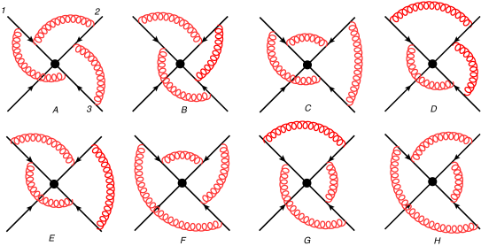
Figure 8: The (2,2,2) web connecting three Wilson lines at three-loop order.

5.1 The (2,2,2) web

The (2,2,2) web potentially contributes to all four colour factors in the basis of eq. (81). As a consequence, one may write the unsubtracted web as

$$W_{(2,2,2)}\left(\alpha_{12},\alpha_{23},\alpha_{13}\right)\,=\,\sum_{i=1}^{4}c_{i}^{(3)}\,{\cal F}_{(2,2,2);i}\left(\alpha_{12},\alpha_{23},\alpha_{13},\epsilon\right)\,.$$ (82)

The combinations of kinematic factors accompanying each colour factor are collected in Table 2. These form the web kernel, which is then combined with appropriate commutators, to form the subtracted web. We present the details of this calculation in appendix B, while here we discuss the results.

Using the specified colour basis the subtracted web takes the form

$$\overline{w}_{(2,2,2)}\left(\alpha_{12},\alpha_{23},\alpha_{13}\right)\,=\,\left(\frac{1}{4\pi}\right)^{3}\,\sum_{i=1}^{4}\,c_{i}^{(3)}\,F_{(2,2,2);i}\left(\alpha_{12},\alpha_{23},\alpha_{13}\right)\,,$$ (83)

where

$$F_{(2,2,2);i}\left(\alpha_{12},\alpha_{23},\alpha_{13}\right) = \int_{0}^{1}dx_{1}dx_{2}dx_{3}\,p_{0}(x_{1},\alpha_{12})\,p_{0}(x_{2},\alpha_{23})\,p_{0}(x_{3},\alpha_{13})$$

$$\hskip 14.22636pt\times\,{\cal G}_{(2,2,2);i}\left(x_{1},x_{2},x_{3},q(x_{1},\alpha_{12}),q(x_{2},\alpha_{23}),(x_{3},\alpha_{13})\right)\,.$$

The subtracted web kernels ${\cal G}_{(2,2,2);i}$, defined in eq. (42), will be given below. Note that, in contrast to the two-line cases analysed in the previous section, where ${\cal G}_{W}$ depends only on the $x_{i}$ variables, here the subtracted web kernel depends on $q(x_{i},\alpha_{ij})$ as well: this dependence is related to the presence of subdivergences in these webs. We will see that the subtracted web kernels depend on their arguments via powers of logarithms only, as anticipated in Ref. Gardi:2013saa . This simple structure emerges through the cancellation of all polylogarithms amongst the various diagrams and commutators, when the subtracted web kernel is assembled (see for example eq. (B.1) and eqs. (B.2) through (B.2), respectively). This simplification is responsible for the factorized structure of the final result.

To express the subtracted web kernels in compact form, we define the logarithmic functions

$$L_{ij}\,\equiv\,\log\left(\frac{q(x_{i},\alpha_{ij})}{x_{i}^{2}}\right)\,;\qquad R_{i}\,\equiv\,\log\left(\frac{x_{i}}{1-x_{i}}\right)\,.$$ (85)

In terms of these functions, the subtracted web kernels associated to the first three colour factors are

$${\cal G}_{(2,2,2),\,1}^{(3)} = \frac{1}{3}\,\bigg{[}R_{2}^{2}-\frac{1}{4}L_{23}^{2}+\frac{1}{8}L_{12}^{2}+\frac{1}{8}L_{31}^{2}+\frac{1}{4}L_{12}L_{23}-\frac{1}{2}L_{31}L_{12}+\frac{1}{4}L_{23}L_{31}\bigg{]}\,,$$

$${\cal G}_{(2,2,2),\,2}^{(3)} = \frac{1}{3}\,\bigg{[}R_{3}^{2}-\frac{1}{4}L_{31}^{2}+\frac{1}{8}L_{23}^{2}+\frac{1}{8}L_{12}^{2}+\frac{1}{4}L_{23}L_{31}-\frac{1}{2}L_{12}L_{23}+\frac{1}{4}L_{31}L_{12}\bigg{]}\,,$$ (86)

$${\cal G}_{(2,2,2),\,3}^{(3)} = -\,\frac{1}{3}\,\bigg{[}R_{1}^{2}-\frac{1}{4}L_{12}^{2}+\frac{1}{8}L_{23}^{2}+\frac{1}{8}L_{31}^{2}+\frac{1}{4}L_{31}L_{12}-\frac{1}{2}L_{23}L_{31}+\frac{1}{4}L_{12}L_{23}\bigg{]}\,.$$

As expected from Bose symmetry in eq. (83), the three functions ${\cal G}_{(2,2,2),\,i}^{(3)}$ can be obtained from each other by permuting the relevant indices; the overall sign for $i=3$ compared to $i=1$ and $2$ reflects the symmetry properties of the corresponding colour factors in eq. (81) under cyclic permutations.

In contrast to eq. (5.1), the contribution of the (2,2,2) web to the fully antisymmetric colour factor $c^{(3)}_{4}$ is found to vanish,

$${\cal G}_{(2,2,2),\,4}^{(3)}\,=\,0\,.$$ (87)

One sees explicitly that each subtracted web kernel consists of products of logarithms involving distinct kinematic invariants, consistent with the basis of functions defined in Sec. 4. It is now straightforward to integrate the results over the ‘angle’ parameters $x_{i}$. In line with eq. (37), we denote the integrated coefficient of each colour factor (with factors of $(4\pi)^{3}$ removed) by $F_{(2,2,2),\,i}^{(3)}$; the result for the first kinematic factor is then

Colour Factor	Kinematic Feynman Integral ${\cal F}_{(2,2,2),\,i}$
$c_{1}^{(3)}$	$\frac{1}{12}(-2A-2B+C-2D+E-2F+G+H)$
$c_{2}^{(3)}$	$\frac{1}{12}(-2A-2B-2C+D+E+F-2G+H)$
$c_{3}^{(3)}$	$\frac{1}{12}(2A+2B-C-D+2E-F-G+2H)$
$c_{4}^{(3)}$	$\frac{1}{2}(-A+B)$

Table 2: Kinematic integral associated with each colour factor in the (2,2,2) web of Fig. 8, where $A\equiv{\cal F}(A)$ and similarly for $B,C$, etc.

$$F^{(3)}_{(2,2,2),\,1}\left(\alpha_{12},\alpha_{23},\alpha_{13}\right) = \frac{1}{3}\,r(\alpha_{12})r(\alpha_{23})r(\alpha_{13})\,\times$$

$$\bigg{[}-\,M_{0,0,0}(\alpha_{12})M_{0,0,0}(\alpha_{13})\bigg{(}\frac{1}{4}\,M_{2,0,0}(\alpha_{23})-\,M_{0,2,0}(\alpha_{23})\bigg{)}$$

$$+\frac{1}{8}\,M_{0,0,0}(\alpha_{13})M_{0,0,0}(\alpha_{23})M_{2,0,0}(\alpha_{12})$$

$$+\,\frac{1}{8}\,M_{0,0,0}(\alpha_{12})M_{0,0,0}(\alpha_{23})M_{2,0,0}(\alpha_{13})-\frac{1}{2}\,M_{0,0,0}(\alpha_{23})M_{1,0,0}(\alpha_{12})M_{1,0,0}(\alpha_{13})$$

$$+\,\frac{1}{4}\,M_{0,0,0}(\alpha_{13})M_{1,0,0}(\alpha_{12})M_{1,0,0}(\alpha_{23})+\frac{1}{4}\,M_{0,0,0}(\alpha_{12})M_{1,0,0}(\alpha_{13})M_{1,0,0}(\alpha_{23})\bigg{]}\,.$$

The second and third kinematic contributions may be obtained via

$$F^{(3)}_{(2,2,2),\,2}\left(\alpha_{12},\alpha_{23},\alpha_{13}\right) = F^{(3)}_{(2,2,2),\,1}\left(\alpha_{23},\alpha_{13},\alpha_{12}\right)\,,$$

$$F^{(3)}_{(2,2,2),\,3}\left(\alpha_{12},\alpha_{23},\alpha_{13}\right) = -\,F^{(3)}_{(2,2,2),\,1}\left(\alpha_{13},\alpha_{12},\alpha_{23}\right)\,,$$ (89)

as follows from the symmetry of the web, and the relabelling of the colour factors in eq. (81). Finally, the fourth kinematic factor vanishes

$$F^{(3)}_{(2,2,2),\,4}\,=\,0\,,$$ (90)

as is clear from the vanishing of the subtracted web kernel in eq. (87). One may note that the subtracted kernels ${\cal G}_{(2,2,2),\,i}^{(3)}$ do not contain any Heaviside function, despite the fact that individual diagrams (given in Appendix B) contain one for every Wilson line. As a consequence, only a subclass of the basis functions is relevant: those without any power of $\ln\widetilde{q}(x,\alpha)$.

Let us now discuss the collinear reduction process, following Sec. 2.2, in the context of the (2,2,2) web. We will see that the above results can be derived from the (1,2,2,1) web of Fig. 4. Indeed, upon taking external lines 1 and 4 to be collinear, one ends up with the diagram of Fig. 9(a), involving a symmetric combination of one-gluon vertices on line 1. Applying the collinear reduction according to eq. (19), the colour factor corresponds to $c_{1}^{(3)}$ of eq. (81). Eqns. (57) and (58), with $\alpha_{34}\rightarrow\alpha_{13}$, then yield

$$\overline{w}^{(3)}_{(1,2,2,1)}\left(\alpha_{12},\alpha_{23},\alpha_{34}\right)\begin{array}[]{c}\\ \longrightarrow\\ _{1||4}\end{array}\,-\,\frac{1}{6}\,f_{abe}f^{e}_{\phantom{e}cd}\,\,\frac{1}{2}\big{\{}T_{1}^{a},T_{1}^{d}\big{\}}\,T_{2}^{b}\,T_{3}^{c}\,\,\left(\frac{1}{4\pi}\right)^{3}r(\alpha_{12})\,r(\alpha_{23})\,r(\alpha_{31})$$ (94)

$$\hskip 170.71652pt\times\,G_{(1,2,2,1)}\left(\alpha_{12},\alpha_{23},\alpha_{31}\right)\,$$ (95)

$$\hskip 85.35826pt=\,-\,c_{1}^{(3)}\,\frac{1}{12}\left(\frac{1}{4\pi}\right)^{3}r(\alpha_{12})\,r(\alpha_{23})\,r(\alpha_{31})\,\,G_{(1,2,2,1)}\left(\alpha_{12},\alpha_{23},\alpha_{31}\right)\,,$$

which indeed agrees with eq. (5.1).

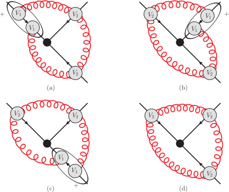
Figure 9: Effective vertex diagrams for the (2,2,2) web. The first three cases, $a,b$ and $c$, can be obtained via collinear reduction from the (1,2,2,1) web of figure 4 and its permutations.

The contributions to the colour factors $c_{2}^{(3)}$ and $c_{3}^{(4)}$ arise from permuting external lines in Fig. 4, as was done in eq. (5.1), so clearly these can also be obtained via collinear reductions of the (1,2,2,1) web. The only contribution that cannot be generated in this way is the effective vertex diagram of Fig. 9(d), which features a $V_{2}$ vertex on all three lines. As explained in Sec. 2, diagrams which feature a single effective vertex on each line constitute the genuinely new information in a given web, that cannot be obtained from collinear reductions of webs connecting more external lines. In the present case, however, the colour factor of the diagram in Fig. 9(d) is the fully antisymmetric combination $c_{4}^{(3)}$, and we have seen above that the kinematic function associated with this colour structure vanishes. The reason for this is that the kinematic function associated with $c_{4}^{(3)}$ involves only diagrams $A$ and $B$ in Fig. 8, in the antisymmetric combination ${\cal F}(A)-{\cal F}(B)$. Diagrams $A$ and $B$, which were referred to as Escher staircase diagrams in Ref. Gardi:2010rn , are special for several reasons: they are highly symmetric, they are chiral enantiomers of each other, and they are fully irreducible: one cannot shrink any gluon to the origin without also pulling in the others. Therefore, they have no subdivergences, and they do not need any commutator counterterms. Finally, their kinematic parts are equal, so that the antisymmetric combination vanishes.

In Sec. 7, we will be able to construct the kinematic integrals of the Escher staircases to all loop orders, and we will prove that a similar cancellation (though with slightly different mechanisms for even and odd numbers of gluons) happens for any number of gluons. More precisely, we will show that, out of $n+1$ colour structures sampled by the $(2^{n})$ web, the only one which cannot be obtained from collinear reduction of $(1,2^{n-1},1)$ webs, which corresponds to a product of $n$ effective vertices of type $V_{2}$, receives contributions only from the two Escher staircases which are present for any $n$, and these contributions cancel, so that the corresponding kinematic function vanishes. Note however that this discussion does not imply that staircase diagrams do not enter the exponent at all. Indeed, as can be seen in Table 2, they do contribute to the colour factors $c_{i}^{(3)}$, with $1\leq i\leq 3$.

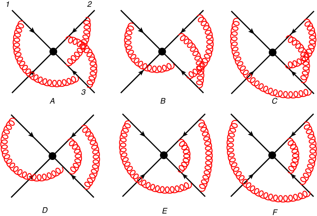
Figure 10: The (1,2,3) web connecting three Wilson lines at three-loop order.

5.2 The (1,2,3) web

In this section we focus on the (1,2,3) web of Fig. 10. Analogously to the (2,2,2) web of the previous section, one may write the unsubtracted web as

$$W_{(1,2,3)}\left(\alpha_{13},\alpha_{23}\right)\,=\,\sum_{i=1}^{4}c_{i}^{(3)}\,{\cal F}_{(1,2,3),\,i}\left(\alpha_{13},\alpha_{23},\epsilon\right)\,.$$ (96)

The combinations of kinematic functions of individual diagrams required for each colour factor are collected in Table 3, and the details of the calculation of the subtracted web may be found in Appendix C. Here we quote the results.

Note first that according to Table 3 this web, in the present basis, has no projection on the $c_{1}^{(3)}$ colour factor. We can therefore consider only the three components $c_{i}^{(3)}$ for $i=2,3,4$. The subtracted web is given by

$$\overline{w}_{(1,2,3)}\left(\alpha_{13},\alpha_{23}\right)\,=\,\left(\frac{1}{4\pi}\right)^{3}\,\sum_{i=2}^{4}c_{i}^{(3)}\,F_{(1,2,3);\,i}\left(\alpha_{13},\alpha_{23}\right)\,,$$ (97)

where

$$F_{(1,2,3);\,i}\left(\alpha_{13},\alpha_{23}\right) = \int_{0}^{1}dx_{1}dx_{2}dx_{3}\,\,p_{0}(x_{1},\alpha_{13})\,p_{0}(x_{2},\alpha_{23})\,p_{0}(x_{3},\alpha_{23})$$

$$\,\quad\times\,{\cal G}_{(1,2,3);\,i}\left(x_{1},x_{2},x_{3},q(x_{1},\alpha_{13}),q(x_{2},\alpha_{23}),q(x_{3},\alpha_{23})\right)\,.$$

The subtracted kernels are

Colour Factor	Kinematic Feynman Integral ${\cal F}_{(1,2,3),\,i}$
$c^{(3)}_{1}$	$0$
$c^{(3)}_{2}$	$\frac{1}{12}(2A-B-C-D+2E-F)$
$c^{(3)}_{3}$	$-\frac{1}{12}(4A+B+C+D-2E+F)$
$c^{(3)}_{4}$	$-\frac{1}{2}(B-C)$

Table 3: Kinematic Feynman integrals accompanying each connected colour factor for the (1,2,3) web of Fig. 10, where $A\equiv{\cal F}(A)$, etc.

$${\cal G}_{(123),\,2}^{(3)} = \frac{1}{3}\bigg{[}\frac{1}{8}L_{13}^{2}-\frac{1}{8}L_{23}^{2}+\frac{1}{4}L_{23}L_{32}-\frac{1}{4}L_{13}L_{23}\bigg{]}\,,$$

$${\cal G}_{(123),\,3}^{(3)} = -\frac{1}{3}\bigg{[}\frac{1}{4}L_{23}L_{13}-\frac{1}{4}L_{23}L_{32}+\frac{1}{8}L_{23}^{2}-\frac{1}{8}L_{13}^{2}-R_{2}^{2}\bigg{]}\,,$$ (99)

$${\cal G}_{(1,2,3),4}^{(3)} = \frac{2}{3}\,\theta(x_{2}-x_{3})\bigg{[}\,2\,L_{13}R_{2}+L_{23}\left(R_{3}-R_{2}\right)$$

$$\hskip 28.45274pt-\,\log^{2}\left(\frac{x_{2}}{x_{3}}\right)+\log\left(\frac{x_{2}}{x_{3}}\right)\log\left(\frac{1-x_{2}}{1-x_{3}}\right)\bigg{]}\,,$$

where we used the definitions in eq. (85). As a consequence of the presence of two entangled gluons spanning the cusp between lines 2 and 3, all subtracted kernels have a leftover Heaviside function; for the first two colour structures, it has been eliminated using symmetries of the integrand in the variables $(x_{1},x_{2},x_{3})$, while this cannot be done for the coefficient of $c_{4}^{(3)}$. This not withstanding, the final integration can be performed, and the result can be expressed in terms of our basis functions. Indeed, given the above subtracted kernels, we find

$$F^{(3)}_{(1,2,3),\,2}(\alpha_{13},\alpha_{23}) = \frac{1}{12}\,r(\alpha_{13})r^{2}(\alpha_{23})\bigg{[}\frac{1}{2}\,M_{2,0,0}(\alpha_{13})M_{0,0,0}^{2}(\alpha_{23})$$ (100a)

$$-\,\frac{1}{2}\,M_{2,0,0}(\alpha_{23})M_{0,0,0}(\alpha_{13})M_{0,0,0}(\alpha_{23})+M_{0,0,0}(\alpha_{13})M^{2}_{1,0,0}(\alpha_{23})$$

$$-\,M_{0,0,0}(\alpha_{23})M_{1,0,0}(\alpha_{13})M_{1,0,0}(\alpha_{23})\bigg{]}\,,$$

$$F^{(3)}_{(1,2,3),\,3}(\alpha_{13},\alpha_{23}) = -\,\frac{1}{12}\,r(\alpha_{13})r^{2}(\alpha_{23})\bigg{[}-\frac{1}{2}\,M_{2,0,0}(\alpha_{13})M_{0,0,0}^{2}(\alpha_{23})$$

$$+\,\frac{1}{2}\Big{(}M_{2,0,0}(\alpha_{23})-8M_{0,2,0}(\alpha_{23})\Big{)}M_{0,0,0}(\alpha_{13})M_{0,0,0}(\alpha_{23})$$

$$-\,M_{0,0,0}(\alpha_{13})M_{1,0,0}^{2}(\alpha_{23})+M_{0,0,0}(\alpha_{23})M_{1,0,0}(\alpha_{13})M_{1,0,0}(\alpha_{23})\bigg{]}\,,$$

$$F_{(1,2,3),\,4}^{(3)}(\alpha_{13},\alpha_{23}) = \frac{4}{3}\,r(\alpha_{13})r^{2}(\alpha_{23})\bigg{[}M_{0,1,1}(\alpha_{23})M_{1,0,0}(\alpha_{13})$$

$$+\frac{1}{8}\,\Big{(}M_{1,0,0}^{2}(\alpha_{23})-M_{0,0,0}(\alpha_{23})M_{2,0,0}(\alpha_{23})-\frac{1}{12}\,M_{0,0,0}^{4}(\alpha_{23})$$

$$+\,2\,M_{0,0,0}(\alpha_{23})M_{0,2,0}(\alpha_{23})\Big{)}M_{0,0,0}(\alpha_{13})\bigg{]}\,.$$

As for the (2,2,2) web, and the MGEWs discussed in the previous section, these results are fully consistent with our expectations: the kinematic functions entering the anomalous dimension take the form of a sum of products of polylogarithmic functions of individual cusp angles, consistently with the factorization conjecture of Ref. Gardi:2013saa , and these functions all belong to the basis of eq. (53). The way this is realised in the case of the (1,2,3) web is non-trivial: this web includes two cusp angles and these are entangled in individual diagrams due to three Heaviside functions. We find again that polylogarithms appear in the kernel of individual diagrams and in the unsubtracted web, but not in the subtracted web kernel. Furthermore, the only Heaviside function surviving in the subtracted web kernel ${\cal G}_{(1,2,3),4}^{(3)}$ in eq. (5.2) relates two of the angular integrations associated with the same kinematic variable $\alpha_{23}$, and therefore is consistent with the factorization property.

We conclude by discussing the constraints provided by collinear reduction. As for the (2,2,2) web discussed above, one may obtain certain components of the (1,2,3) web from collinear reductions of webs connecting four Wilson lines. Two of the three components of eq. (97) can be obtained this way: the component associated with the colour factor $c_{2}^{(3)}$ corresponds, in the effective vertex description, to diagram (a) in Fig. 11, and can be obtained by collinear reduction from the (1,1,3,1) web, while the component associated with colour factor $c_{3}^{(3)}$ corresponds to diagram (b) in Fig. 11, and can be obtained by collinear reduction from the (1,2,2,1) web. The component of $c_{4}^{(3)}$ corresponds, in turn, to diagram (c); since the latter has a single effective vertex on each line, it cannot be obtained through collinear reduction.

Let us now examine the two components that can be deduced from four-line webs. In the case of diagram (a) in Fig. 11, one may first permute lines 3 and 4 in the result of the (1,1,1,3) web, so that the line carring the $V_{3}$ vertex will be line $3$, matching our conventions for the (1,2,3) web. Following this permutation, we apply the collinear reduction by identifying line $4$ with line $2$. To match diagram (a) in Fig. 11 we must also include a symmetry factor of $1/2$, associated with the exchange of the two gluons, both propagating between the $V_{3}$ vertex on line 3 and the $V_{1}$ vertices on line $2$: this symmetry factor is absent in the original (1,1,3,1) web, where the two gluons attach to different lines. We thus get

$$\overline{w}^{(3)}_{(1,1,3,1)}\left(\alpha_{13},\alpha_{23},\alpha_{34}\right)\begin{array}[]{c}\\ \longrightarrow\\ _{4||2}\end{array} -\frac{1}{2}\times\frac{1}{6}\,\,T_{1}^{a}\,\frac{1}{2}\,\big{\{}T_{2}^{b},T_{2}^{d}\big{\}}\,T_{3}^{c}\left(\frac{1}{4\pi}\right)^{3}r(\alpha_{13})\,r^{2}(\alpha_{23})$$

$$\times\,\Big{[}f_{ace}f^{e}_{\phantom{e}bd}\,G_{(1,1,1,3)}\left(\alpha_{13},\alpha_{23},\alpha_{23}\right)+f_{ade}f^{e}_{\phantom{e}bc}\,G_{(1,1,1,3)}\left(\alpha_{23},\alpha_{13},\alpha_{23}\right)\Big{]}$$

$$=\,-\frac{1}{6}\,T_{1}^{a}\,\frac{1}{2}\,\big{\{}T_{2}^{b},T_{2}^{d}\big{\}}\,T_{3}^{c}\left(\frac{1}{4\pi}\right)^{3}r(\alpha_{13})\,r^{2}(\alpha_{23})\,f_{ade}f^{e}_{\phantom{e}bc}\,G_{(1,1,1,3)}\left(\alpha_{23},\alpha_{13},\alpha_{23}\right)\,,$$

where in the last line we kept only the second term, noting that the first vanishes owing to the contraction of the colour tensors. It is straightforward to check, using eq. (60), that eq. (5.2) reproduces the $c_{2}^{(3)}$ component of the (1,2,3) web in eq. (97), with the kinematic function given by eq. (100a).

Finally, consider diagram (b) in Fig. 11. This diagram can be obtained from the collinear reduction of the (1,2,2,1) web of eq. (57) by identifying lines $3$ and $1$, and then renaming $4$ as $1$, to match our conventions for the (1,2,3) web. One finds

$$\overline{w}^{(3)}_{(1,2,2,1)}\left(\alpha_{12},\alpha_{23},\alpha_{34}\right)\begin{array}[]{c}\\ \longrightarrow\\ _{1||3}\end{array} -\frac{1}{6}\,f_{abe}f^{e}_{\phantom{e}cd}\,T_{1}^{d}\,T_{2}^{b}\,\frac{1}{2}\,\big{\{}T_{3}^{a},T_{3}^{c}\big{\}}\left(\frac{1}{4\pi}\right)^{3}r^{2}(\alpha_{23})\,r(\alpha_{13})$$ (110)

$$\hskip 56.9055pt\times\,G_{(1,2,2,1)}\left(\alpha_{23},\alpha_{23},\alpha_{13}\right)\,.$$

One may verify, using eq. (58), that this equation exactly reproduces eq. (97), with the kinematic function given by eq. (100).

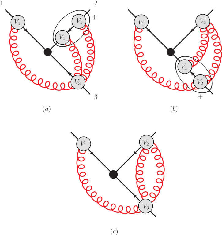
Figure 11: The three components of the (1,2,3) web using the effective vertex formalism. The components described by the two upper diagrams can be obtained via collinear reduction of: (a) the (1,1,3,1) web; (b) the (1,2,2,1) web. Diagram (c) shows the connected colour factor that features one vertex on each line and cannot be determined by collinear reduction.

In this section, we have calculated the three-loop, three-line MGEWs that are needed for the three-loop soft anomalous dimension. In the remainder of the paper, we examine how the methods developed here, and in Ref. Gardi:2013saa , can be applied beyond the three-loop order. We begin by studying a particular four-loop example in the following section.

6 A four-loop, five-line web

The method developed in Ref. Gardi:2013saa and in Sections 2-4 above allows us to compute high-order webs in the MGEW class with relatively little effort. It is then worthwhile to look for interesting examples beyond three loops: this will provide non-trivial checks of our conjectures on the analytic structure of subtracted webs, and on the relevant basis of functions.

In this Section, we present for the first time a complete calculation of a fully subtracted four-loop web. As our example, we choose to consider the (1,2,2,2,1) web, connecting five Wilson lines at four loops, and consisting of the diagrams depicted in Fig. 12. The (1,2,2,2,1) web is particularly interesting because of its simple colour structure, and because, spanning five legs, it will allow one to determine certain components of other webs at the same order, spanning a smaller number of Wilson lines but having more than one effective vertex on at least one line. Furthermore, the (1,2,2,2,1) web is the third member of the infinite series of MGEWs (1,2,2,$\cdots$,2,1), connecting $n+1$ lines at $n$ loops. All the webs in this class have a single colour structure, and the general solution of the corresponding web mixing matrices for any $n$ have been obtained using combinatorial methods in Dukes:2013wa ; Dukes:2013gea , while the kinematic functions have been determined in Gardi:2013saa for the cases $n=2,3$. One may hope that a completely explicit answer for the first three elements of this collection could provide some insights for an all-order answer.

The pattern of subtractions at the four-loop level is particularly intricate, as can be seen from eq. (2.1). For example, in the specific case of the web (1,2,2,2,1), we need to consider the commutators of the webs (1,2,2,1), (1,2,1) and (1,1) connecting the five lines. In this section we organize and discuss the result, while further details are given in Appendix D.

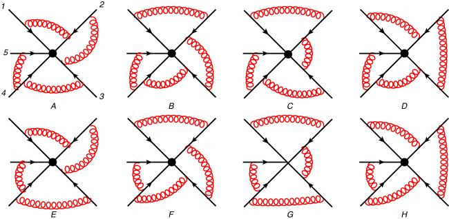
Figure 12: The (1,2,2,2,1) web connecting five Wilson lines at four loops.

The first step in the construction of the subtracted web is the determination of the colour structure. In the case of the (1,2,2,2,1) web, depicted in Fig. 12, there is only one colour structure, which can be written in terms of ordinary colour generators as

$$c_{1}^{(5)}\,=\,T^{a}_{1}\,\big{[}T^{a}_{2},T^{b}_{2}\big{]}\,\big{[}T^{b}_{3},T^{c}_{3}\big{]}\big{[}T^{c}_{4},T^{d}_{4}\big{]}T^{d}_{5}\,.$$ (111)

The corresponding combination of integrals can be constructed from the appropriate web mixing matrix, which is known Dukes:2013gea . Expressing the result in terms of the kinematic Feynman integrals of the individual diagrams in Fig. 12, one finds

$${\cal F}^{(4)}_{(1,2,2,2,1),\,1}\left(\alpha_{ij},\epsilon\right) = \frac{1}{24}\,\left[6\left({\cal F}^{(4)}(F)-{\cal F}^{(4)}(A)\right)+2\left({\cal F}^{(4)}(C)+{\cal F}^{(4)}(D)+{\cal F}^{(4)}(E)\right)\right.$$ (112)

$$\left.-2\left({\cal F}^{(4)}(B)+{\cal F}^{(4)}(G)+{\cal F}^{(4)}(H)\right)\right]\,.$$

It is convenient to work at the level of the integrand of the diagrams, by taking directly the combination in eq. (112) of the functions $\phi_{X}^{(4)}$ given in Appendix D. The unsubtracted web is lengthy, and, much like the (1,2,2,1) web of Ref. Gardi:2013saa , contains polylogarithms, so upon integration it does not yield a factorised function of the cusp angles, but rather a lengthy sum of Goncharov polylogarithms involving different kinematic variables.

According to the factorisation conjecture, we expect that the commutators of the webs at lower orders will cancel all the correlations between different cusp angles, as well as all polylogarithmic functions in the kernel. We find that indeed the integrand of the subtracted web becomes much simpler, and the integrated result is factorised as expected. The subtracted web kernel, in terms of the functions defined in eq. (85), is given by

$${\cal G}^{(4)}_{(1,2,2,2,1),\,1}\big{(}x_{i},q(x_{i},\alpha_{i})\big{)} = -\,\frac{1}{144}\bigg{\{}L_{12}^{3}-3L_{23}^{3}+3L_{34}^{3}-L_{45}^{3}$$

$$+\,\,3L_{12}^{2}\bigg{[}L_{23}+L_{34}-3L_{45}\bigg{]}-3L_{45}^{2}\bigg{[}L_{23}+L_{34}-3L_{12}\bigg{]}$$

$$+\,3L_{23}^{2}\bigg{[}L_{12}-3L_{34}+5L_{45}\bigg{]}-3L_{34}^{2}\bigg{[}L_{45}-3L_{23}+5L_{12}\bigg{]}$$

$$+\,6\bigg{[}L_{12}L_{23}L_{34}-3L_{12}L_{23}L_{45}+3L_{12}L_{34}L_{45}-L_{23}L_{34}L_{45}\bigg{]}$$

$$+\,24\bigg{[}R_{2}^{2}\,\bigg{(}L_{12}+L_{23}+L_{34}-3L_{45}\bigg{)}-R_{3}^{2}\,\bigg{(}L_{23}+L_{34}+L_{45}-3L_{12}\bigg{)}\bigg{]}\bigg{\}}\,.$$

By looking at the subtracted web kernel in eq. (6), we immediately note that the result is already expressed in terms of the functions of the basis in eq. (53). More precisely, the functions $M_{3,0,0}(\alpha_{ij})$ and $M_{1,2,0}(\alpha_{ij})$ at weight four are the only new functions appearing at this order. Upon performing the $x_{k}$ integrals, and in the notations of eq. (42), we find that the contribution of this web to the anomalous dimension is given by

$$F^{(4)}_{(1,2,2,2,1),1}\left(\alpha_{ij}\right)=-\,\frac{1}{144}\,r(\alpha_{12})r(\alpha_{23})r(\alpha_{34})r(\alpha_{45})\times$$ (114)

$$\times\bigg{\{}\bigg{[}6\bigg{(}M_{1,0,0}(\alpha_{12})M_{1,0,0}(\alpha_{23})M_{1,0,0}(\alpha_{34})M_{0,0,0}(\alpha_{45})$$

$$\hskip 14.22636pt-\,\,3M_{1,0,0}(\alpha_{12})M_{1,0,0}(\alpha_{23})M_{1,0,0}(\alpha_{45})M_{0,0,0}(\alpha_{34})\bigg{)}$$

$$\hskip 14.22636pt+\,\,\bigg{(}M_{3,0,0}(\alpha_{12})M_{0,0,0}(\alpha_{45})-9M_{2,0,0}(\alpha_{12})M_{1,0,0}(\alpha_{45})\bigg{)}M_{0,0,0}(\alpha_{23})M_{0,0,0}(\alpha_{34})$$

$$\hskip 14.22636pt-\,\,3\bigg{(}M_{3,0,0}(\alpha_{23})M_{0,0,0}(\alpha_{34})+3M_{2,0,0}(\alpha_{23})M_{1,0,0}(\alpha_{34})\bigg{)}M_{0,0,0}(\alpha_{12})M_{0,0,0}(\alpha_{45})$$

$$\hskip 14.22636pt+\,\,3M_{2,0,0}(\alpha_{12})M_{0,0,0}(\alpha_{45})\bigg{(}M_{1,0,0}(\alpha_{23})M_{0,0,0}(\alpha_{34})+M_{1,0,0}(\alpha_{34})M_{0,0,0}(\alpha_{23})\bigg{)}$$

$$\hskip 14.22636pt+\,\,3M_{2,0,0}(\alpha_{23})M_{0,0,0}(\alpha_{34})\bigg{(}M_{1,0,0}(\alpha_{12})M_{0,0,0}(\alpha_{45})+5M_{1,0,0}(\alpha_{45})M_{0,0,0}(\alpha_{12})\bigg{)}$$

$$\hskip 14.22636pt+\,\,24M_{0,2,0}(\alpha_{23})\bigg{(}M_{1,0,0}(\alpha_{12})M_{0,0,0}(\alpha_{34})M_{0,0,0}(\alpha_{45})$$

$$\hskip 14.22636pt+M_{1,0,0}(\alpha_{34})M_{0,0,0}(\alpha_{12})M_{0,0,0}(\alpha_{45})-\,\,3M_{1,0,0}(\alpha_{45})M_{0,0,0}(\alpha_{12})M_{0,0,0}(\alpha_{34})\bigg{)}+$$

$$\hskip 14.22636pt24M_{1,2,0}(\alpha_{23})M_{0,0,0}(\alpha_{12})M_{0,0,0}(\alpha_{34})M_{0,0,0}(\alpha_{45})\bigg{]}$$

$$\hskip 14.22636pt-\,\,\bigg{[}(\alpha_{12}\leftrightarrow\alpha_{45}),(\alpha_{23}\leftrightarrow\alpha_{34})\bigg{]}\bigg{\}}\,.$$

As expected, we find a factorized function of uniform transcendental weight ${\rm w}=7$, expressed as a sum of products of our basis functions, each one depending on a single cusp angle, and satisfying the symbol conjecture. Through various collinear limits, this will also yield information on other four-loop webs, involving less than five Wilson lines, but with more than one effective vertex on a given line.

7 The Escher Staircase and (2, 2, …, 2) webs

In this section we would like to display the flexibility and the reach of the formalism that we have developed by computing a certain class of diagrams contributing to a specific series of MGEW’s to all orders in perturbation theory. The results of the calculation are not of immediate physical relevance, since we will not be computing complete webs, much less subtracted webs, to all orders. Nevertheless, the calculation of these particular diagrams will allow us to prove a general statement about this series of webs. Moreover, the feasibility of this calculation suggests that all-order calculations of MGEWs are possible. In addition the simplicity of the result, which by itself is properly factorized into functions belonging to our basis, provides further evidence for our conjectures.

Following Ref. Gardi:2010rn , we dub the class of diagrams we will compute ‘Escher staircases’, for reasons that should be apparent from their graphical structure. An example with $n=6$ is displayed in Fig. 13. These diagrams are the most symmetric members of the $n$-loop $(2,2,\ldots,2)$ webs: each such web contains $2^{n}$ diagrams, two of which are of the form we are studying, differing by clockwise or counterclockwise orientations. The staircase diagrams are particularly interesting, not only because of their graphical symmetry, but also because they do not have subdivergences, so they do not require commutator counterterms. As a consequence, they should satisfy the alphabet and factorization conjectures by themselves, and indeed we will find that they do.

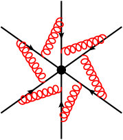
Figure 13: Example of an Escher staircase with six external legs. There are two staircases at arbitrary order, related by reflection.

Interestingly, we also find that a non-trivial cancellation takes place when the kinematic factors of staircase diagrams are combined to build up contributions to the $n$-loop soft anomalous dimension. Indeed, as verified in Sec. 5.1 for the (2,2,2) web, the two staircases are the only diagrams to contribute to the colour structure composed of only $V_{2}$ effective vertices, denoted by $c_{4}^{(3)}$ in Sec. 5.1. Their contributions to that colour structure however cancel exactly, as noted in eq. (90). The (2,2,2) staircases of course do contribute to the other three colour structures, $c_{i}^{(3)}$, with $i=1,2,3$. One should keep in mind, however, that the kinematic functions of those colour structures can be obtained also from collinear reduction of the $(1,2,2,1)$ web. A similar story is played out for the $(2,2,\ldots,2)$ web at arbitrary order, and we provide a general argument for this in what follows.

Turning now to the evaluation of the Escher staircase at $n$ loops, we begin by noticing that the diagram kernel in eq. (30) can be explicitly written down, for the staircase, as

$$\phi_{S}^{(n)}\left(x_{i};\,\epsilon\right) = \int_{0}^{1}\prod_{k=1}^{n-1}dy_{k}\,\left(1-y_{k}\right)^{-1+2\epsilon}\,y_{k}^{-1+2k\epsilon}\,$$ (115)

$$\times\,\prod_{i=1}^{n}\,\theta\left[\left(1-x_{i}\right)\left(1-y_{i-1}\right)\prod_{j=i}^{n-1}y_{j}-x_{i+1}\left(1-y_{i}\right)\prod_{j=i+1}^{n-1}y_{j}\right]\,,$$

where the $i$-th Heaviside function guarantees that the absorption point of gluon $i-1$ is further away (along Wilson line $i$) than the emission point of gluon $i$. To properly define the product of $\theta$ functions, we set $1-y_{0}=1-y_{n}=1$ when they occur, as well as $\prod_{j=n+1}^{n-1}y_{j}=\prod_{j=1}^{n-1}y_{j}$ in the last factor, and $\prod_{j=n}^{n-1}y_{j}=1$ in the penultimate factor; similarly, we set $x_{n+1}=x_{1}$ when it occurs. To illustrate the notation, we write explicitly the products of $\theta$ functions for small $n$, as

$$n=2\quad \rightarrow \quad\theta\left[(1-x_{1})\,y_{1}-x_{2}\,(1-y_{1})\right]\theta\left[(1-x_{2})(1-y_{1})-x_{1}\,y_{1}\right]\,,$$

$$n=3\quad \rightarrow \quad\theta\left[(1-x_{1})\,y_{1}\,y_{2}-x_{2}\,(1-y_{1})\,y_{2}\right]\,\theta\left[(1-x_{2})(1-y_{1})\,y_{2}-x_{3}\,(1-y_{2})\right]$$ (116)

$$\quad\theta\left[(1-x_{3})(1-y_{2})-x_{1}\,y_{1}\,y_{2}\right]\,,$$

$$n=4\quad \rightarrow \quad\theta\left[(1-x_{1})\,y_{1}\,y_{2}\,y_{3}-x_{2}\,(1-y_{1})\,y_{2}\,y_{3}\right]$$

$$\quad\theta\left[(1-x_{2})(1-y_{1})\,y_{2}\,y_{3}-x_{3}\,(1-y_{2})\,y_{3}\right]\,\theta\left[(1-x_{3})(1-y_{2})\,y_{3}-x_{4}\,(1-y_{3})\right]$$

$$\quad\theta\left[(1-x_{4})(1-y_{3})-x_{1}\,y_{1}\,y_{2}\,y_{3}\right]\,.$$

Using the fact that $0<x_{i}<1$, and $0<y_{i}<1$, it is easy to realize that the $\theta$ functions are more naturally expressed by changing variables to $\xi_{i}\equiv y_{i}/(1-y_{i})$, so that $0<\xi_{i}<\infty$. In this way one gets, for small $n$, factors of

$$n=2\quad \rightarrow \quad\theta\left[\frac{x_{2}}{1-x_{1}}<\xi_{1}<\frac{1-x_{2}}{x_{1}}\right]\,\theta\left[\frac{(1-x_{1})(1-x_{2})}{x_{1}x_{2}}>1\right]\,,$$

$$n=3\quad \rightarrow \quad\theta\left[\frac{x_{3}}{1-x_{2}}<\xi_{2}<\frac{1-x_{3}}{x_{1}\xi_{1}}\right]\,\theta\left[\frac{x_{2}}{1-x_{1}}<\xi_{1}<\frac{(1-x_{2})(1-x_{3})}{x_{1}x_{3}}\right]$$ (117)

$$\quad\theta\left[\frac{(1-x_{1})(1-x_{2})(1-x_{3})}{x_{1}x_{2}x_{3}}>1\right]\,,$$

$$n=4\quad \rightarrow \quad\theta\left[\frac{x_{4}}{1-x_{3}}<\xi_{3}<\frac{(1-x_{4})(1+\xi_{1})}{x_{1}\xi_{1}\xi_{2}}\right]\,\theta\left[\frac{x_{3}}{1-x_{2}}<\xi_{2}<\frac{(1-x_{3})(1-x_{4})}{x_{1}x_{4}\xi_{1}}\right]$$

$$\quad\theta\left[\frac{x_{2}}{1-x_{1}}<\xi_{1}<\frac{(1-x_{2})(1-x_{3})(1-x_{4})}{x_{1}x_{3}x_{4}}\right]$$

$$\quad\theta\left[\frac{(1-x_{1})(1-x_{2})(1-x_{3})(1-x_{4})}{x_{1}x_{2}x_{3}x_{4}}>1\right]\,,$$

where we used the notation $\theta(a<x<b)$ to denote the product $\theta(b-x)\,\theta(x-a)$. Furthermore, the last $\theta$ function for each $n$ must be present since the variables $x_{i}$ must also later be integrated in the interval $0<x_{i}<1$; its meaning is clear: it distinguishes the ‘clockwise’ staircase diagram from the ‘counterclockwise’ one, which carries the complementary $\theta$ function. We define therefore

$$\theta_{+}(n)\,\equiv\,\theta\Big{(}S_{n}(x_{i})-1\Big{)}\,$$ (118)

where

$$S_{n}(x_{i})\,\equiv\,\prod_{i=1}^{n}\frac{1-x_{i}}{x_{i}}\,.$$ (119)

The $n$-loop ‘clockwise’ staircase diagram carries a factor of $\theta_{+}(n)$, while its ‘counterclockwise’ image carries a factor of $\theta_{-}(n)=1-\theta_{+}(n)$. Upon further inspection of eq. (7) one sees also that the $\xi_{i}$ integrals are all bounded from above and from below: since poles in $\epsilon$ could only arise from the limits $\xi_{i}\to\{0,\infty\}$, this implies, as expected, that the staircase graph has only a single overall ultraviolet divergence, given by $\Gamma(2n\epsilon)$ in eq. (3.1), and no subdivergences. It is not difficult to work out the generalization to all $n$ of the constraints in eq. (7): one can then write eq. (115) as

$$\phi_{S}^{(n)}\left(x_{i};\,\epsilon\right) = \int_{0}^{\infty}\prod_{k=1}^{n-1}d\xi_{k}\left(1+\xi_{k}\right)^{-2(k+1)\epsilon}\,\xi_{k}^{-1+2k\epsilon}\,\,\Theta_{S}\big{[}\left\{x_{k},\xi_{k}\right\}\big{]}$$

$$= \theta_{+}(n)\int_{A_{1}}^{B_{1}}\frac{d\xi_{1}}{\xi_{1}}\,\int_{A_{2}}^{B_{2}\left(\xi_{1}\right)}\frac{d\xi_{2}}{\xi_{2}}\,\,\ldots\,\int_{A_{n-1}}^{B_{n-1}\left(\xi_{1},\xi_{2},\ldots,\xi_{n-2}\right)}\frac{d\xi_{n-1}}{\xi_{n-1}}\,+\,{\cal O}\left(\epsilon\right)\,.$$

Importantly, the resulting integral is explicitly of a ‘$d\log$’ form, in agreement with the considerations of Refs. Henn:2013wfa ; Gardi:2013saa . The remaining difficulty is that (also as expected) the integrals are nested and not completely factorized. One can however work out explicitly the limits of integration, generalizing eq. (7). One finds

$$A_{k}\,=\,\frac{x_{k+1}}{1-x_{k}}\,,\qquad B_{k}\left(\xi_{1},\ldots\xi_{k-1}\right)\,=\,\frac{\prod_{j=k+1}^{n}(1-x_{j})}{\prod_{j=k+2}^{n+1}x_{j}}\,\frac{\prod_{j=1}^{k-2}(1+\xi_{j})}{\prod_{j=1}^{k-1}\xi_{j}}\,,$$ (121)

where we define $x_{n+1}=x_{1}$, and all products running over empty sets of integers are set equal to one. The final integration is now trivial, and one finds the remarkably simple result

$$\phi_{S}^{(n)}\left(x_{i};\,0\right)\,=\,\frac{1}{(n-1)!}\,\,\theta_{+}(n)\,\bigg{(}\log\Big{[}S_{n}(x_{i})\Big{]}\bigg{)}^{n-1}\,.$$ (122)

The result is Bose symmetric and completely factorized, and, when integrated to give the kinematic function ${\cal F}^{(n)}(S)$ of eq. (3.1), manifestly expressible in terms of our basis functions.

Note now that by sending $x_{i}\leftrightarrow 1-x_{i}$ in eq. (122), the result has the same form, but with a factor $(-1)^{n-1}$ from the power of the logarithm, and $\theta_{+}$ replaced by $\theta_{-}$. Denoting the clockwise and anticlockwise staircase diagrams by $S_{+}$ and $S_{-}$ respectively, one thus finds

$${\cal F}(S_{+})\,=\,(-1)^{n-1}{\cal F}(S_{-})\,.$$ (123)

This leads to the cancellation observed at three loops ($n=3$) in Sec. 5.1: the two staircase diagrams have identical kinematic factors, which however combine to form the coefficient of the colour structure $c_{3}^{(4)}$ with the same weight and opposite signs. Since the other diagrams in the (2,2,2) web do not contribute to $c_{3}^{(4)}$, the corresponding coefficient vanishes. We now argue that a similar argument applies in an arbitrary $(2,2,\ldots,2)$ web.

Let us define a colour basis for $n$-loop webs connecting $n$ lines, generalising the 3-loop basis of eq. (81). The requirement in constructing this basis is that it should allow one to express all the colour components of the (2,2,$\ldots$,2) web. The dimension of this basis is $n+1$, and its elements have a transparent interpretation (see Fig. 9 for the three-loop case) upon considering the (2,2,$\ldots$,2) web in the effective vertex formalism of Ref. Gardi:2013ita : $c_{i}^{(n)}$ ($1\leq i\leq n$) is the colour factor one obtains upon having two $V_{1}$ vertices on line $i$, corresponding to an anticommutator of colour generators, and a $V_{2}$ vertex, corresponding to a commutator, on all the other lines, yielding

$$c_{i}^{(n)}\,=\,\left[T_{1}^{a_{1}},T_{1}^{a_{2}}\right]\left[T_{2}^{a_{2}},T_{2}^{a_{3}}\right]\ldots\left\{T_{i}^{a_{i}},T_{i}^{a_{i+1}}\right\}\ldots\left[T_{n-1}^{a_{n-1}},T_{n-1}^{a_{n}}\right]\left[T_{n}^{a_{n}},T_{n}^{a_{1}}\right]\,.$$ (124)

Finally, the $n+1$-st basis element is the fully antisymmetric colour factor corresponding to a $V_{2}$ vertex on each of the lines,

$$c_{n+1}^{(n)}\,=\,\left[T_{1}^{a_{1}},T_{1}^{a_{2}}\right]\left[T_{2}^{a_{2}},T_{2}^{a_{3}}\right]\ldots\left[T_{n-1}^{a_{n-1}},T_{n-1}^{a_{n}}\right]\left[T_{n}^{a_{n}},T_{n}^{a_{1}}\right]\,.$$ (125)

It is this latter component of the $(2,2,\ldots,2)$ web that will receive a contribution from the kinematic integrals of the staircase diagrams only, which will ultimately turn out to vanish. First, one notes that the fact that staircase diagrams are irreducible means that the web mixing matrix has the generic form

$$\left(\begin{array}[]{ccc}1&0&\ldots\\ 0&1&\ldots\\ 0&0&\ldots\\ \vdots&\vdots&\ldots\\ 0&0&\ldots\end{array}\right),$$

where the first two columns arise from the staircase diagrams. This form follows from the replica trick analysis of Ref. Gardi:2010rn , which dictates that the exponentiated colour factor of diagram $D$ receives no contributions from diagrams $D^{\prime}$ which are more reducible (less irreducible) than $D$. From the above form, it then follows that any such mixing matrix has right-eigenvectors of the form

$$\left(\begin{array}[]{cccccc}a&b&0&0&\ldots&0\end{array}\right)\,,$$ (126)

for arbitrary $a$ and $b$. Two special cases are $a=\pm b=1$, corresponding to the symmetric and antisymmetric combinations of $S_{+}$ and $S_{-}$. These combinations are special in that they have definite parity under a “flipping transformation” that interchanges all pairs of gluons on all lines simultaneously. Such a transformation exchanges $S_{+}\rightarrow S_{-}$, and so the symmetric (anti-symmetric) combination has flipping parity $+$ ($-$) respectively. The contribution from the entire web must be invariant under this transformation, as it maps the total web to itself. Given that the basis of colour factors in eqs. (124) and (125) is linearly independent, each separate colour factor multiplied by the corresponding kinematic function must also be invariant under the flipping transformation. The basis we have chosen is particularly convenient in this regard, as each colour factor has a definite flipping parity: $(-1)^{n-1}$ for $c_{i}^{(n)}$ ($1\leq i\leq n$) and $(-1)^{n}$ for the fully antisymmetric colour factor $c_{n+1}^{(n)}$. One then finds that the contribution to the latter colour factor contains the combination

$$c_{n+1}^{(n)}\left[{\cal F}(S_{+})-{\cal F}(S_{-})+\ldots\right]\,,$$

for odd $n$, and

$$c_{n+1}^{(n)}\left[{\cal F}(S_{+})+{\cal F}(S_{-})+\ldots\right]\,,$$

for even $n$, where the ellipsis in each case denotes possible contributions from non-staircase diagrams. In fact, such contributions are not present, which can be seen as follows. At the $n$-loop order, there are $n+1$ colour factors, $n$ of which have parity $(-1)^{n-1}$, and only one of which has parity $(-1)^{n}$. It follows that of the $(n+1)$ right eigenvectors with eigenvalue 1, $n$ must correspond to kinematic functions with flipping parity $(-1)^{n-1}$, and only one to parity $(-1)^{n}$. Since we know that the eigenvector of eq. (126) with $a=(-1)^{n}b$ has parity $(-1)^{n}$, this must be the only possibility, and there can be no other contributions. Having established eq. (123) above, this completes the proof that the contribution to the fully antisymmetric colour factor from the $(2,2,\ldots,2)$ web vanishes.

Returning to consider the (2,2,$\ldots$ 2) $n$-th order web as a whole, we now see that all of its non-vanishing components belong to the colour structures in eq. (124), where one of the lines features an anticommutator of two $V_{1}$ emission vertices. This means that it may be determined from the corresponding $n$-loop $n+1$ line (1,2,2,$\ldots$ 2,1) web through collinear reduction, just as the (2,2,2) web was obtained from the (1,2,2,1) web in eq. (57). Specifically, at four-loops we essentially have the result for the (2,2,2,2) web based on the calculation of the (1,2,2,2,1) web in Sec. 6.

In this section, we have shown that is possible to calculate a particular type of web diagram to all orders in perturbation theory. As seen from the explicit calculations of other webs, the computations for diagrams with sudivergences are considerably more intricate, and further technical developments will be needed before a complete calculation of an all-order class of subtracted webs can be completed. The present example however testifies to the underlying simplicity of the structure of MGEWs, and suggests that the problem of computing this class of webs might at some point be completely solved.

8 Conclusion

In this paper, we have extended the programme of Refs. Gardi:2010rn ; Gardi:2011yz ; Gardi:2013ita ; Gardi:2013saa , which established a diagrammatic approach for studying infrared singularities in QCD scattering amplitudes (see also Mitov:2010rp ; Vladimirov:2014wga ). We have done this by computing the ultraviolet singularities of products of semi-infinite Wilson lines in terms of webs. In the multi-line case, webs are sets of diagrams, each closed under the group of gluon permutations on the Wilson lines, whose contribution to the exponent of the Wilson line correlator consists of a sum of terms, each involving a fully connected colour factor multiplying a linear combination of Feynman integrals of diagrams belonging to the set. As explained in detail in Refs. Gardi:2011yz ; Gardi:2013ita ; Gardi:2013saa , and reviewed here, each web contains ultraviolet subdivergences in general, which must be removed by appropriate counterterms involving commutators of subdiagrams. This makes the case of multi-leg scattering qualitatively different to the familiar case of a Wilson loop; we call the combination of an unrenormalised web and its counterterms a subtracted web.

Specifically, we have focused on the contribution to the soft anomalous dimension from diagrams consisting of multiple gluon exchanges between the Wilson lines. These Multi-Gluon Exchange Webs (MGEWs) are the simplest diagrams at any given order; however, they also contain the highest number of ultraviolet subdivergences. Thus, the web language, coupled with a suitable infrared regulator for calculating individual diagrams, is extremely useful in order to cleanly isolate their contribution to the soft anomalous dimension.

MGEWs connecting four Wilson lines at three-loop order were already considered in Ref. Gardi:2013saa , which also analysed the analytic structure of MGEWs in general. It was conjectured that: (i) the contributions of MGEWs to the soft anomalous dimension take the form of sums of products of polylogarithmic functions, each involving a single cusp angle; (ii) the symbol alphabet of these functions consists of $\{\alpha_{ij},\alpha/(1-\alpha_{ij}^{2})\}$, where $\alpha_{ij}$ is defined in eq. (2) as the exponent of the cusp angle formed between lines $i$ and $j$.

In this paper we provided significant additional evidence supporting these conjectures. Moreover, we took a step forward in understanding MGEWs by constructing a basis of functions, motivated by the alphabet conjecture as well as specific calculations, that we conjecture can be used to express MGEWs connecting any number of Wilson lines at arbitrary order in perturbation theory. The basis $M_{k,l,n}(\alpha)$, is defined in eq. (53) as a single parameter integral over the gluon emission angle. The integrand consists of a product of three types of logarithms (depending on the gluon emission angle and the corresponding cusp angle) raised to non-negative integer powers $k,l$ and $n$, respectively. The basis functions are consistent with the alphabet conjecture, and they are conveniently characterised by their symbols; these are listed in Table 1 up to weight 5. The functions may also be explicitly evaluated in terms of Harmonic polylogarithms with indices $0$ and $1$: all independent functions up to weight 5 are listed in Appendix A. The three logarithms appearing in the integrands of $M_{k,l,n}(\alpha)$ have been identified in two-loop calculations of the (2,2) and (1,2,1) webs, where functions up to weight 3 appear, that is $M_{k,l,n}(\alpha)$ with $k+n+l\leq 2$. The basis passed all tests at three loops, where basis elements up weight $5$ appear, corresponding to $k+n+l\leq 4$. These tests include the four-line webs of Ref. Gardi:2013saa , namely the (1,2,2,1) and (1,1,1,3) webs, the three-line webs of Sec. 5 above, namely the (2,2,2) and (1,2,3) webs, as well as the two-line (3,3) web of Sec. 4.2. Further tests are provided by the five-line four-loop (1,2,2,2,1) web computed in Sec. 6, and by the all order analysis of the Escher Staircase diagrams and the (2,2,$\ldots$,2) webs in Sec. 7.

Another important result of the present paper is the discovery of the collinear reduction relations between webs connecting different numbers of Wilson lines. These relations, which we briefly summarise below, are discussed in more detail in Sec. 2, and then illustrated in several examples throughout the paper. The idea is formulated using the effective vertex language of Ref. Gardi:2013ita , which provides a convenient colour basis for webs. In this language, the emission of $K$ gluons from a Wilson line, associated with a tree-graph colour factor (a fully nested commutator) is described by an effective vertex $V_{K}$. Considering a given web, different components may be described as connected graphs made out of such vertices, as shown for example in Figs. 7, 9 and 11. These graphs may in general feature one or more effective vertices on a given line. However, when multiple vertices appear on a line, they are not ordered: the integrals range over the entire Wilson line independently of each other, and in the colour factor one takes the symmetric combination of all possible orderings. As a consequence, the calculation of such a graph maps directly into the calculation of a graph where the Wilson line that features several vertices is replaced by a set of collinear lines, each featuring only one of these vertices. The upshot is that starting with a web that features a single effective vertex on each line, one may deduce various components of webs connecting fewer Wilson lines, but featuring more than one vertex on some of the lines. Collinear reduction provides stringent checks of the two- and three-line webs computed in this paper: it allowed us to determine one of the two components of the (3,3) web in eq. (75), and the entire (2,2,2) web in eq. (94), from the (1,2,2,1) web, as well as two of the three components of the (1,2,3) web in eqs. (110) and (5.2), using, respectively, the (1,2,2,1) and (1,1,3,1) webs. We note that the only colour component that cannot be deduced by collinear reduction for the (1,2,3) web is the one corresponding to the fully antisymmetric colour factor $c_{4}^{(3)}$ in eq. (81). Given that the same diagrams enter both the components that can be deduced by collinear reduction and those that cannot, webs connecting less than the maximal number of lines at a given order are strongly constrained, providing us with high confidence in the results presented in this paper.

As an additional check on the basis of functions we propose, as well as to illustrate the power and general applicability of the web language, we have also calculated the (1,2,2,2,1) four-loop web, and the Escher Staircase diagrams to arbitrary order in perturbation theory. The latter enter the (2,2,…,2) web, and are especially simple because they do not contain ultraviolet subdivergences. Furthermore, we were able to show that the component corresponding to the fully antisymmetric colour factor of the (2,2,…,2) web vanishes. This was proven using the fact that this colour structure is associated exclusively with the Escher Staircase diagrams, and these two diagrams are related by a parity transformation as in eq. (123). The conclusion is rather striking: the entire contribution of the (2,2,…,2) web family to the exponent can be deduced from the corresponding (1,2,2,…,2,1) webs through collinear reduction. Specifically, at four loops, the result for the (2,2,2,2) web can be directly read off the results of Sec. 6 for the (1,2,2,2,1) web.

The analysis and explicit calculations performed in this paper promote our understanding of an entire class of contributions to the renormalization of Wilson line correlators. The progress achieved in understanding the analytic properties of the result Gardi:2013saa , and the specific class of functions by which they may be expressed, is a step towards translating the entire calculation of an arbitrary MGEW into a combinatorial problem: given the factorization conjecture and the basis of functions, along with the expected transcendental weight, one may write down an ansatz for the answer where only rational numerical coefficients need to be fixed. This, along with the progress already made on webs Gardi:2010rn ; Gardi:2011yz ; Gardi:2013ita and their combinatorics Gardi:2011wa ; Dukes:2013wa ; Dukes:2013gea may facilitate all-order calculations in the future.

The results of this paper also constitute a further step forward in assembling all necessary ingredients for the soft anomalous dimension of massive partons at three-loop order. In order to complete this programme, one needs to include MGEWs in which gluons can be emitted and absorbed from the same Wilson line. Furthermore, one needs to include diagrams containing a single three-gluon vertex off the Wilson lines, and those fully connected graphs which contain two three-gluon vertices or a single four-gluon vertex. Work in these directions is ongoing Gardi:2014kpa .

Acknowlegments

EG and CDW are supported by the Science and Technologies Facilities Council (STFC). MH is supported by the University of Edinburgh. CDW, LM and GF thank the Higgs Centre for Theoretical Physics for warm hospitality, and MH thanks the University of Torino and INFN, Torino for support and hospitality. Work supported by MIUR (Italy), under contract 2010YJ2NYW$\_$006 and by the University of Torino and the Compagnia di San Paolo under contract ORTO11TPXK. The authors would like to thank Jenni Smillie for help and collaboration on related topics, and Claude Duhr and Øyvind Almelid for making available their codes for the treatment of polylogarithmic functions, and for useful discussions.

Appendix A Basis Functions

In this appendix we list the explicit expressions for the basis functions defined in eq. (53), in terms of polylogarithms and harmonic polylogarithms, up to transcendental weight five. Harmonic polylogarithms are defined as in Remiddi:1999ew .

• Weight one.

  $$\begin{split}M_{0,0,0}(\alpha)\,=\,2\log(\alpha)\,.\end{split}$$ (127)

• Weight two.

  $$\begin{split}M_{1,0,0}(\alpha)\,=\,2\,\text{Li}_{2}(\alpha^{2})+4\log(\alpha)\log\left(1-\alpha^{2}\right)-2\log^{2}(\alpha)-2\,\zeta(2).\end{split}$$ (128)

• Weight three.

  $$\begin{split}M_{0,0,2}(\alpha)\,=\,\frac{8}{3}\log^{3}(\alpha)\,,\end{split}$$ (129)

  $$\begin{split}M_{0,1,1}(\alpha)\,=\,2\,\text{Li}_{3}(\alpha^{2})-2\log(\alpha)\bigg{[}\text{Li}_{2}(\alpha^{2})+\frac{\log^{2}(\alpha)}{3}+\zeta(2)\bigg{]}-2\,\zeta(3)\,,\end{split}$$ (130)

  $$\begin{split}M_{0,2,0}(\alpha)\,=\,\frac{2}{3}\log^{3}(\alpha)+4\,\zeta(2)\,\log(\alpha)\,,\end{split}$$ (131)

  $$\begin{split}M_{2,0,0}(\alpha)&=-\,4\,\bigg{[}\text{Li}_{3}(\alpha^{2})+2\text{Li}_{3}\left(1-\alpha^{2}\right)\bigg{]}-8\log\left(1-\alpha^{2}\right)\log^{2}(\alpha)\\ &+\,\frac{8}{3}\,\log^{3}(\alpha)+8\,\zeta(2)\,\log(\alpha)+4\,\zeta(3)\,.\end{split}$$ (132)

• Weight four.

  $$\begin{split}M_{3,0,0}(\alpha)&=\,12\,\bigg{[}\text{Li}_{4}(\alpha^{2})-4\,\text{Li}_{4}\left(1-\alpha^{2}\right)\bigg{]}-24\,S_{2,2}(\alpha^{2})\\ &-\,24\,\log\left(1-\alpha^{2}\right)\,\text{Li}_{3}(\alpha^{2})-24\,\log^{2}\left(1-\alpha^{2}\right)\,\log^{2}(\alpha)\\ &+\,16\,\log\left(1-\alpha^{2}\right)\,\log^{3}(\alpha)-\,4\,\log^{4}(\alpha)\\ &-\,24\,\zeta(2)\,\log(\alpha)\,\log\left[\frac{\alpha}{\left(1-\alpha^{2}\right)^{2}}\right]\\ &+\,24\,\zeta(3)\,\log\left[\alpha\left(1-\alpha^{2}\right)\right]-\,6\,\zeta(4)\,,\end{split}$$ (133)

  $$\begin{split}M_{1,2,0}(\alpha)&=\,4\,\text{Li}_{4}(\alpha^{2})-4\,\log(\alpha)\,\text{Li}_{3}(\alpha^{2})+2\,\log^{2}(\alpha)\,\text{Li}_{2}(\alpha^{2})\\ &+\,\frac{4}{3}\,\log^{3}(\alpha)\,\log\left(1-\alpha^{2}\right)-\,\frac{2}{3}\,\log^{4}(\alpha)\\ &+\,\zeta(2)\,\Big{[}8\,\log(\alpha)\log\left(1-\alpha^{2}\right)+4\,\text{Li}_{2}(\alpha^{2})-6\,\log^{2}(\alpha)\Big{]}\\ &+\,4\,\zeta(3)\,\log(\alpha)-14\,\zeta(4)\,,\end{split}$$ (134)

  $$\begin{split}M_{1,0,2}(\alpha)&=\,4\,\text{Li}_{4}(\alpha^{2})-8\,\log(\alpha)\,\text{Li}_{3}(\alpha^{2})+8\,\log^{2}(\alpha)\,\text{Li}_{2}(\alpha^{2})\\ &+\frac{16}{3}\,\log^{3}(\alpha)\,\log\left(1-\alpha^{2}\right)-\,\frac{4}{3}\,\log^{4}(\alpha)-4\,\zeta(4)\,,\end{split}$$ (135)

  $$\begin{split}M_{1,1,1}(\alpha)&=-\,4\,\text{Li}_{4}(\alpha^{2})+4\,S_{2,2}(\alpha^{2})+2\,\log\left[\alpha\left(1-\alpha^{2}\right)^{2}\right]\,\text{Li}_{3}(\alpha^{2})\\ &+\,4\,\log(\alpha)\,\text{Li}_{3}\left(1-\alpha^{2}\right)\\ &-\,\frac{4}{3}\,\log(\alpha)^{2}\,\log\left(1-\alpha^{2}\right)\bigg{[}\log(\alpha)-3\,\log\left(1-\alpha^{2}\right)\bigg{]}\\ &-\,8\,\zeta(2)\,\log(\alpha)\log(1-\alpha^{2})-2\,\zeta(3)\,\log\left[\alpha\left(1-\alpha^{2}\right)^{2}\right]+3\,\zeta(4)\,.\end{split}$$ (136)

• Weight five

  $$\begin{split}M_{0,0,4}(\alpha)\,=\,\frac{32}{5}\,\log^{5}(\alpha)\,,\end{split}$$ (137)

  $$\begin{split}M_{4,0,0}(\alpha)&=\,48\,H_{0,0,0,1,0}(\alpha^{2})+96\,H_{1,0,0,1,0}(\alpha^{2})+96\,H_{0,1,0,1,0}(\alpha^{2})\\ &+\,48\,H_{0,0,1,0,0}(\alpha^{2})+96\,H_{0,0,1,1,0}(\alpha^{2})+192\,H_{1,1,0,1,0}(\alpha^{2})\\ &+\,96\,H_{1,0,1,0,0}(\alpha^{2})+192\,H_{1,0,1,1,0}(\alpha^{2})+48\,H_{0,1,0,0,0}(\alpha^{2})\\ &+\,96\,H_{0,1,1,0,0}(\alpha^{2})+192\,H_{0,1,1,1,0}(\alpha^{2})+48\,H_{1,0,0,0,0}(\alpha^{2})\\ &+\,96\,H_{1,1,0,0,0}(\alpha^{2})+192\,H_{1,1,1,0,0}(\alpha^{2})+384\,H_{1,1,1,1,0}(\alpha^{2})\\ &+\,\frac{32}{5}\,\log^{5}(\alpha)+64\,\zeta(2)\,\log^{3}\left(\frac{\alpha}{1-\alpha^{2}}\right)\\ &-96\,\zeta(3)\bigg{[}\zeta(2)+\log^{2}\left(\frac{\alpha}{1-\alpha^{2}}\right)\bigg{]}\\ &+\,432\,\zeta(4)\,\log\frac{\alpha}{1-\alpha^{2}}-144\,\zeta(5)\,,\end{split}$$ (138)

  $$\begin{split}M_{0,4,0}(\alpha)&=\,\frac{2}{5}\,\log^{5}(\alpha)+8\,\zeta(2)\,\log^{3}(\alpha)+84\,\zeta(4)\,\log(\alpha)\,,\end{split}$$ (139)

  $$\begin{split}M_{0,1,3}(\alpha)&=\,-\,6\,H_{0,0,0,1,0}(\alpha^{2})-6\,H_{0,0,1,0,0}(\alpha^{2})-6\,H_{0,1,0,0,0}(\alpha^{2})\\ &-\,\frac{12}{5}\,\log^{5}(\alpha)-8\,\zeta(2)\,\log^{3}(\alpha)-12\,\zeta(3)\,\log^{2}(\alpha)\\ &-\,12\,\zeta(4)\,\log(\alpha)-12\,\zeta(5)\,,\end{split}$$ (140)

  $$\begin{split}M_{0,3,1}(\alpha)&=\,-\frac{3}{2}\,\bigg{[}H_{0,0,0,1,0}(\alpha^{2})+H_{0,1,0,0,0}(\alpha^{2})\bigg{]}-\frac{2}{5}\,\log^{5}(\alpha)\\ &+\,6\,\zeta(2)\,\Big{[}-\log^{3}(\alpha)-2\,\log(\alpha)\,\text{Li}_{2}(\alpha^{2})+2\,\text{Li}_{3}(\alpha^{2})\Big{]}\\ &-\,6\,\zeta(3)\,\log^{2}(\alpha)-42\,\zeta(4)\,\log(\alpha)-12\,\zeta(2)\,\zeta(3)-12\,\zeta(5)\,,\end{split}$$ (141)

  $$\begin{split}M_{2,2,0}(\alpha)&=\,4\,H_{0,0,0,1,0}(\alpha^{2})+4\,H_{1,0,0,1,0}(\alpha^{2})+4\,H_{0,0,1,1,0}(\alpha^{2})\\ &+\,4\,H_{1,0,0,0,0}(\alpha^{2})+4\,H_{1,1,0,0,0}(\alpha^{2})+2\,H_{0,1,0,0,0}(\alpha^{2})\\ &+\,2\,H_{0,0,1,0,0}(\alpha^{2})+\,\frac{16}{15}\,\log^{5}(\alpha)\\ &+\,8\,\zeta(2)\,\bigg{[}\log^{2}(\alpha)\bigg{(}2\,\log(\alpha)-3\,\log\left(1-\alpha^{2}\right)\bigg{)}\\ &\hskip 51.21495pt-\,\log(\alpha)\,\text{Li}_{2}(\alpha^{2})-2\,\text{Li}_{3}\left(1-\alpha^{2}\right)\bigg{]}\\ &+\,4\,\zeta(3)\,\bigg{[}2\,\text{Li}_{2}(\alpha^{2})+\log(\alpha)\,\bigg{(}4\,\log\left(1-\alpha^{2}\right)-3\,\log(\alpha)\bigg{)}\bigg{]}\\ &+\,2\,\zeta(4)\,\bigg{[}67\,\log(\alpha)-8\,\log\left(1-\alpha^{2}\right)\bigg{]}-16\,\zeta(5)\,,\end{split}$$ (142)

  $$\begin{split}M_{2,0,2}(\alpha)&=\,8\,H_{0,1,0,0,0}(\alpha^{2})+8\,H_{1,0,0,0,0}(\alpha^{2})+16\,H_{1,1,0,0,0}(\alpha^{2})\\ &+\,\frac{16}{15}\,\log^{5}(\alpha)+16\,\zeta(4)\,\log\left(\frac{\alpha}{1-\alpha^{2}}\right)\\ &+\,16\,\zeta(2)\zeta(3)-8\,\zeta(5)\,,\end{split}$$ (143)

  $$\begin{split}M_{2,1,1}(\alpha)&=\,-\,4\,H_{0,0,0,1,0}(\alpha^{2})-8\,H_{1,0,0,1,0}(\alpha^{2})-8\,H_{0,1,0,1,0}(\alpha^{2})\\ &-2\,H_{0,0,1,0,0}(\alpha^{2})-8\,H_{0,0,1,1,0}(\alpha^{2})-8\,H_{1,1,0,1,0}(\alpha^{2})\\ &-4\,H_{1,0,1,0,0}(\alpha^{2})-8\,H_{1,0,1,1,0}(\alpha^{2})-4\,H_{0,1,0,0,0}(\alpha^{2})\\ &-4\,H_{0,1,1,0,0}(\alpha^{2})-8\,H_{0,1,1,1,0}(\alpha^{2})-4\,H_{1,1,0,0,0}(\alpha^{2})+\frac{4}{15}\,\log^{5}(\alpha)\\ &-8\,\zeta(2)\bigg{[}\log(\alpha)\bigg{(}2\,\text{Li}_{2}(\alpha^{2})+\,\log^{2}\left(1-\alpha^{2}\right)\bigg{)}-\text{Li}_{3}(\alpha^{2})\bigg{]}\\ &-4\,\zeta(3)\bigg{[}3\,\log^{2}(\alpha)+2\,\log^{2}\left(1-\alpha^{2}\right)-2\,\log(\alpha)\,\log\left(1-\alpha^{2}\right)\bigg{]}\\ &-6\,\zeta(4)\,\Big{[}5\,\log(\alpha)-2\,\log\left(1-\alpha^{2}\right)\Big{]}-8\,\zeta(2)\,\zeta(3)-20\,\zeta(5)\,,\end{split}$$ (144)

  $$\begin{split}M_{0,2,2}(\alpha)&=\,2\,H_{0,0,0,1,0}(\alpha^{2})+4\,H_{0,1,0,1,0}(\alpha^{2})+2\,H_{0,1,0,0,0}(\alpha^{2})\\ &+\frac{16}{15}\,\log^{5}(\alpha)+8\,\zeta(2)\,\bigg{[}\log^{3}(\alpha)+\log(\alpha)\,\text{Li}_{2}(\alpha^{2})-\text{Li}_{3}(\alpha^{2})\bigg{]}\\ &+8\,\zeta(3)\bigg{[}\log^{2}(\alpha)+\text{Li}_{2}(\alpha^{2})\bigg{]}+22\,\zeta(4)\,\log(\alpha)+8\,\zeta(2)\,\zeta(3)+8\,\zeta(5)\,.\end{split}$$ (145)

Appendix B Calculation of the (2,2,2) web

In this appendix, we provide more details regarding the calculation of the (2,2,2) web, the results of which are presented in Sec. 5.1.

B.1 Unsubtracted web

The general method for calculating a given web diagram has been presented in Sec. 3. Here we present the kernels, defined in eq. (3.1) and eq. (30), for each diagram appearing in the (2,2,2) web. To simplify our notations slightly, we relabel the variables used in the Sec. 5.1 as $\{x_{1},x_{2},x_{3}\}\to\{x,y,z\}$. Applying the relevant definitions to the kinematic factor of diagrams $A$ and $B$ in Fig. 8 one finds,

$$\phi^{(3)}_{A}(x,y,z;\epsilon)\,=\,\phi^{(3)}_{B}(x,y,z;\epsilon)\,=\,\frac{1}{4}\log^{2}\left[\frac{x}{1-x}\,\frac{y}{1-y}\,\frac{z}{1-z}\right]+\mathcal{O}(\epsilon)\,,$$ (146)

where we used eqs. (28) and (29). Note that it is necessary to use the symmetry of the function to remove the factor,

$$\theta_{+}(n=3)\,=\,\theta\bigg{(}\frac{1-x}{x}\frac{1-y}{y}\frac{1-z}{z}>1\bigg{)}\,.$$ (147)

The other diagrams in Fig. 8 have subdivergences, therefore the kernels have to be computed including higher orders in their $\epsilon$ expansion. For example, from diagram $C$ one finds

$$\phi^{(3)}_{C}(x,y,z;\epsilon) = \frac{1}{8\epsilon^{2}}\bigg{\{}1+2\,\epsilon\log\left[\frac{(1-y)^{2}(1-z)}{z^{2}x}\right]+\epsilon^{2}\left[24\,{\rm Li}_{2}\left(-\frac{1-y}{z}\right)\right.$$

$$\left.+\,2\,\log^{2}\left(\frac{(1-y)^{2}(1-z)}{z^{2}x}\right)-2\log^{2}\left(\frac{(1-x)(1-y)(1-z)}{xyz}\right)\right]$$

$$+~{}\mathcal{O}(\epsilon^{3})\bigg{\}}\,.$$

The remaining web kernel contributions can then be found by permuting the variables $x$, $y$ and $z$ in the integrand, with the results

$$\phi^{(3)}_{D}(x,y,z;\epsilon) = \phi^{(3)}_{C}(z,x,y;\epsilon)\,,$$

$$\phi^{(3)}_{E}(x,y,z;\epsilon) = \phi^{(3)}_{C}(x,z,y;\epsilon)\,,$$

$$\phi^{(3)}_{F}(x,y,z;\epsilon) = \phi^{(3)}_{C}(y,x,z;\epsilon)\,,$$ (149)

$$\phi^{(3)}_{G}(x,y,z;\epsilon) = \phi^{(3)}_{C}(z,y,x;\epsilon)\,,$$

$$\phi^{(3)}_{H}(x,y,z;\epsilon) = \phi^{(3)}_{C}(y,z,x;\epsilon)\,.$$

From these functions one can compute the unsubtracted web,

$$\begin{split}W_{(2,2,2)}\,=\,\sum_{j=1}^{4}c_{j}^{(3)}\mathcal{F}_{(2,2,2);\,j}^{(3)}\,,\end{split}$$ (150)

using eq. (31) and taking the specific coefficients $Y_{X,j}^{-1}$ given in Table 2. One finds

$$\begin{split}\mathcal{F}_{(2,2,2),j}^{(3)}&=\kappa^{3}\,\Gamma(6\epsilon)\int_{0}^{1}dx\,dy\,dz\,p_{\epsilon}(x,\alpha_{12})p_{\epsilon}(y,\alpha_{23})p_{\epsilon}(z,\alpha_{13})\sum_{X\in(2,2,2)}Y_{X,j}^{-1}~{}\phi_{X}^{(3)}(x,y,z;\epsilon)\\ &=\kappa^{3}\,\Gamma(6\epsilon)\int_{0}^{1}dx\,dy\,dz\,p_{\epsilon}(x,\alpha_{12})p_{\epsilon}(y,\alpha_{23})p_{\epsilon}(z,\alpha_{13})~{}\phi_{(2,2,2),j}^{(3)}(x,y,z;\epsilon)\,.\end{split}$$ (151)

B.2 Subtracted web

As explained in Sec. 2, the anomalous dimension is obtained from subtracted webs. Thus the single pole of eq. (151) must be combined with suitable subtraction terms, consisting of commutators of lower-order webs, as prescribed eq. (11). Recall that simplifications occur Gardi:2013saa when this subtraction is performed under the integral over variables $(x,y,z)$ corresponding to the gluon emission angles. In particular, the symbol alphabet and factorization constraints which allow us to use the basis of functions introduced in section 4 only apply to the subtracted web. Consider then the integrand of eq. (11),

$$\begin{split}\!\overline{w}_{(2,2,2),i}^{(3,-1)}\!=\bigg{(}\frac{1}{4\pi}\bigg{)}^{3}\!\int_{0}^{1}\!dxdydz\,p_{0}(x,\alpha_{12})p_{0}(y,\alpha_{23})p_{0}(z,\alpha_{13})\bigg{(}\mathcal{G}_{0,i}+\sum_{k}\Delta\mathcal{G}_{k,i}\bigg{)}\,,\end{split}$$ (152)

where we defined $\mathcal{G}_{0,i}$ as the contribution proportional to $c_{i}^{(3)}$ from the unsubtracted web, obtained by expanding the integrand of eq. (151); $\Delta\mathcal{G}_{k,i}$, in turn, are the contributions from the commutators of lower order webs to this colour factor, where $k$ runs over the relevant commutator terms in eq. (11) (note that $\Delta\mathcal{G}_{k,i}$ include the numerical factors appearing there). We recall that each of these contributions to $\mathcal{G}_{(2,2,2),i}$ depends on $x,y$ and $z$ as well as on $q(x,\alpha_{12}),q(y,\alpha_{23})$ and $q(z,\alpha_{13})$. Using the lower-order web results collected in Ref. Gardi:2013saa , the contributions to the integrand of $\overline{w}_{(2,2,2)}^{(3)}$ multiplying the colour factor $c_{1}^{(3)}$ are

$$\Delta\mathcal{G}_{\left[w^{(1,0)},w^{(2,-1)}\right],1}\, = \,\,\frac{1}{4}\,\bigg{[}\log\big{[}q(x,\alpha_{12})\big{]}\,\log\left(\frac{y}{z}\right)$$

$$\hskip 34.14322pt-\,\log\big{[}q(z,\alpha_{13})\big{]}\log\left(\frac{x}{y}\right)\bigg{]}\,,$$

$$\Delta\mathcal{G}_{\left[w^{(2,0)},w^{(1,-1)}\right],1}\, = \,-\frac{1}{2}\bigg{[}{\rm Li}_{2}\left(-\frac{y}{z}\right)-{\rm Li}_{2}\left(-\frac{z}{y}\right)$$

$$+\,{\rm Li}_{2}\left(-\frac{y}{x}\right)-{\rm Li}_{2}\left(-\frac{x}{y}\right)$$

$$+\,\frac{1}{2}\log\left(\frac{y}{z}\right)\left(\log\big{[}q(y,\alpha_{23})\big{]}+\log\big{[}q(z,\alpha_{13})]\right)$$

$$-\,\frac{1}{2}\log\left(\frac{x}{y}\right)\left(\log\big{[}q(x,\alpha_{12})\big{]}+\log\big{[}q(y,\alpha_{23})\big{]}\right)\bigg{]}\,,$$

$$\Delta\mathcal{G}_{\big{[}w^{(1,0)},[w^{(1,-1)},w^{(1,0)}]\big{]},1}\, = \,-\frac{1}{12}\,\Big{[}\log\big{[}q(x,\alpha_{12})\big{]}\log\big{[}q(y,\alpha_{23})\big{]}$$

$$+\log\big{[}q(z,\alpha_{13})\big{]}\log\big{[}q(y,\alpha_{23})\big{]}-\,2\log\big{[}q(z,\alpha_{13})\big{]}\log\big{[}q(x,\alpha_{12})\big{]}\Big{]}\,,$$

$$\Delta\mathcal{G}_{\big{[}w^{(1,-1)},[w^{(1,1)},w^{(1,-1)}]\big{]},1}\, = \,-\frac{1}{24}\,\Big{[}\log^{2}\big{[}q(z,\alpha_{13})\big{]}-2\log^{2}\big{[}q(y,\alpha_{23})\big{]}$$

$$\hskip 25.60747pt+\,\log^{2}\big{[}q(x,\alpha_{12})\big{]}\Big{]}\,.$$

The contributions to the coefficient of the colour factor $c^{(3)}_{2}$ are

$$\Delta\mathcal{G}_{\left[w^{(1,0)},w^{(2,-1)}\right],2}\, = \,\,\frac{1}{4}\,\bigg{[}-\log\big{[}q(x,\alpha_{12})\big{]}\,\log\left(\frac{y}{z}\right)\,+\,\,\log\big{[}q(y,\alpha_{23})\big{]}\log\left(\frac{z}{x}\right)\bigg{]}\,,$$

$$\Delta\mathcal{G}_{\left[w^{(2,0)},w^{(1,-1)}\right],2}\, = \,-\frac{1}{2}\bigg{[}{\rm Li}_{2}\left(-\frac{z}{x}\right)-{\rm Li}_{2}\left(-\frac{x}{z}\right)+\,{\rm Li}_{2}\left(-\frac{z}{y}\right)-{\rm Li}_{2}\left(-\frac{y}{z}\right)$$

$$+\,\frac{1}{2}\log\left(\frac{z}{x}\right)\left(\log\big{[}q(z,\alpha_{13})\big{]}+\log\big{[}q(x,\alpha_{12})]\right)$$

$$-\,\frac{1}{2}\log\left(\frac{y}{z}\right)\left(\log\big{[}q(y,\alpha_{23})\big{]}+\log\big{[}q(z,\alpha_{13})\big{]}\right)\bigg{]}\,,$$

$$\Delta\mathcal{G}_{\big{[}w^{(1,0)},[w^{(1,-1)},w^{(1,0)}]\big{]},2}\, = \,-\frac{1}{12}\,\Big{[}\log\big{[}q(x,\alpha_{12})\big{]}\log\big{[}q(z,\alpha_{13})\big{]}$$

$$+\log\big{[}q(z,\alpha_{13})\big{]}\log\big{[}q(y,\alpha_{23})\big{]}-\,2\log\big{[}q(y,\alpha_{23})\big{]}\log\big{[}q(x,\alpha_{12})\big{]}\Big{]}\,,$$

$$\Delta\mathcal{G}_{\big{[}w^{(1,-1)},[w^{(1,1)},w^{(1,-1)}]\big{]},2}\, = \,-\frac{1}{24}\,\Big{[}\log^{2}\big{[}q(y,\alpha_{23})\big{]}-2\log^{2}\big{[}q(z,\alpha_{13})\big{]}$$

$$\hskip 25.60747pt+\,\log^{2}\big{[}q(x,\alpha_{12})\big{]}\Big{]}\,.$$

Finally, the contributions to the coefficient of the colour factor $c_{3}^{(3)}$ are found to be

$$\Delta\mathcal{G}_{\left[w^{(1,0)},w^{(2,-1)}\right],3}\, = \,\,\frac{1}{4}\,\bigg{[}-\log\big{[}q(z,\alpha_{13})\big{]}\,\log\left(\frac{x}{y}\right)$$

$$\hskip 34.14322pt+\,\log\big{[}q(y,\alpha_{23})\big{]}\log\left(\frac{z}{x}\right)\bigg{]}\,,$$

$$\Delta\mathcal{G}_{\left[w^{(2,0)},w^{(1,-1)}\right],3}\, = \,-\frac{1}{2}\bigg{[}{\rm Li}_{2}\left(-\frac{z}{x}\right)-{\rm Li}_{2}\left(-\frac{x}{z}\right)$$

$$+\,{\rm Li}_{2}\left(-\frac{y}{x}\right)-{\rm Li}_{2}\left(-\frac{x}{y}\right)$$

$$+\,\frac{1}{2}\log\left(\frac{z}{x}\right)\left(\log\big{[}q(z,\alpha_{13})\big{]}+\log\big{[}q(x,\alpha_{12})]\right)$$

$$-\,\frac{1}{2}\log\left(\frac{x}{y}\right)\left(\log\big{[}q(x,\alpha_{12})\big{]}+\log\big{[}q(y,\alpha_{23})\big{]}\right)\bigg{]}\,,$$

$$\Delta\mathcal{G}_{\big{[}w^{(1,0)},[w^{(1,-1)},w^{(1,0)}]\big{]},3}\, = \,\,\frac{1}{12}\,\Big{[}\log\big{[}q(x,\alpha_{12})\big{]}\log\big{[}q(y,\alpha_{23})\big{]}$$

$$+\log\big{[}q(z,\alpha_{13})\big{]}\log\big{[}q(x,\alpha_{12})\big{]}-\,2\log\big{[}q(y,\alpha_{23})\big{]}\log\big{[}q(z,\alpha_{13})\big{]}\Big{]}\,,$$

$$\Delta\mathcal{G}_{\big{[}w^{(1,-1)},[w^{(1,1)},w^{(1,-1)}]\big{]},3}\, = \,\,\frac{1}{24}\,\Big{[}\log^{2}\big{[}q(z,\alpha_{13})\big{]}-2\log^{2}\big{[}q(x,\alpha_{12})\big{]}$$

$$\hskip 25.60747pt+\,\log^{2}\big{[}q(y,\alpha_{23})\big{]}\Big{]}\,.$$

There are no commutator counterterms contributing to the fully antisymmetric colour factor $c_{4}^{(3)}$, as there are no colour factors of lower order webs that commute to produce the desired structure. This is consistent with the fact that the kinematic function associated with $c^{(3)}_{4}$ involves only staircase diagrams, which are irreducible, and as such do not contain subdivergences.

Combining all terms, using appropriate dilogarithm identities, and the symmetry of $p_{0}(x,\alpha)$ under $x\leftrightarrow 1-x$, and finally using the definition given in eq. (53), one finds the results presented in eqs. (5.1) and (90). As a check of these results, one may verify that the ${\cal O}(\epsilon^{-2})$ pole of the (2,2,2,) web vanishes, according to the web consistency relation discussed in Ref. Gardi:2011yz ,

$$\left.w^{(3,-2)}\right|_{\beta_{0}=0}\,=\,-\,\frac{1}{6}\left[w^{(1,-1)},w^{(2,-1)}\right]\,.$$ (156)

As a further check, the sum of all web diagrams must give a product of one-loop graphs, in accordance with eq. (34). We have explicitly confirmed that both of these criteria are satisfied.

Appendix C Calculation of the (1,2,3) web

The calculation of the (1,2,3) web, shown in Fig. 10, proceeds similarly to the (2,2,2) case considered in the previous Appendix.

C.1 Unsubtracted web

Using the method of Sec. 3, the result for the contribution to the web kernel $\phi_{(1,2,3)}^{(3)}$ from diagram $A$ is

$$\phi_{A}^{(3)}=\frac{1}{4}\log^{2}\left[\frac{y(1-x)}{x(1-y)}\right]$$ (157)

Carrying out a similar exercise for the other diagrams of the (1,2,3) web gives the results

$$\phi_{B}^{(3)} = \frac{1}{8\epsilon^{2}}\,\theta(x-y)\,\left(\frac{1-x}{z}\right)^{2\epsilon}\bigg{[}\left(\frac{1-y}{1-x}\right)^{4\epsilon}-\left(\frac{y}{x}\right)^{4\epsilon}$$

$$\hskip 56.9055pt+\,24\,\epsilon^{2}\,\left({\rm Li}_{2}\left(-\frac{x}{y}\right)-\,{\rm Li}_{2}\left(-\frac{y}{x}\right)\right)+{\cal O}(\epsilon^{3})\bigg{]}\,,$$

$$\phi_{C}^{(3)} = \frac{1}{2\epsilon}\,\theta(x-y)\left[\frac{\Gamma(2\epsilon)\Gamma(4\epsilon)}{\Gamma(6\epsilon)}-\frac{1}{2\epsilon}\left(\frac{1-y}{z}\right)^{2\epsilon}\right]\left[\left(\frac{1-y}{1-x}\right)^{2\epsilon}-\left(\frac{y}{x}\right)^{2\epsilon}\right]\,,$$

$$\phi_{D}^{(3)} = \frac{1}{8\epsilon^{2}}\left(\frac{1-y}{z}\right)^{2\epsilon}\left[\theta(y-x)\left(\frac{x}{y}\right)^{4\epsilon}+\theta(x-y)\left(\frac{1-x}{1-y}\right)^{4\epsilon}\right.$$

$$\left.+24\,\epsilon^{2}\,\theta(y-x)\,{\rm Li}_{2}\left(-\frac{x}{y}\right)+\,24\,\epsilon^{2}\,\theta(x-y)\,{\rm Li}_{2}\left(-\frac{1-x}{1-y}\right)+{\cal O}(\epsilon^{3})\right]\,,$$

$$\phi_{E}^{(3)} = \frac{1}{8\epsilon^{2}}\left\{\theta(x-y)\left[2\left(\frac{1-x}{z}\right)^{2\epsilon}\left(\frac{1-y}{1-x}\right)^{-2\epsilon}-\left(\frac{1-y}{z}\right)^{2\epsilon}\left(\frac{1-y}{1-x}\right)^{-4\epsilon}\right]\right.$$ (158)

$$\hskip 22.76219pt\left.+\,\theta(y-x)\left[2\left(\frac{1-x}{z}\right)^{2\epsilon}\left(\frac{y}{x}\right)^{-2\epsilon}-\left(\frac{1-y}{z}\right)^{2\epsilon}\left(\frac{y}{x}\right)^{-4\epsilon}\right]\right.$$

$$\left.\hskip 22.76219pt+\,24\,\epsilon^{2}\,{\rm Li}_{2}\left(-\frac{1-x}{z}\right)+{\cal O}(\epsilon^{3})\right\}\,,$$

$$\phi_{F}^{(3)} = \frac{1}{2\epsilon}\Bigg{\{}\theta(x-y)\left(\frac{1-y}{1-x}\right)^{-2\epsilon}\left[\frac{\Gamma(4\epsilon)\Gamma(2\epsilon)}{\Gamma(6\epsilon)}\left(1+8\epsilon^{2}{\rm Li}_{2}\left(-\frac{1-x}{1-y}\right)\right)\right.$$

$$\hskip 17.07164pt\left.-\frac{1}{2\epsilon}\left(\frac{1-x}{z}\right)^{2\epsilon}\left(1+12\epsilon^{2}{\rm Li}_{2}\left(-\frac{1-x}{1-y}\right)\right)\right]$$

$$\hskip 17.07164pt+\,\theta(y-x)\left(\frac{y}{x}\right)^{-2\epsilon}\left[\frac{\Gamma(4\epsilon)\Gamma(2\epsilon)}{\Gamma(6\epsilon)}\left(1+8\epsilon^{2}{\rm Li}_{2}\left(-\frac{x}{y}\right)\right)-\frac{1}{2\epsilon}\left(\frac{1-x}{z}\right)^{2\epsilon}\right.$$

$$\hskip 17.07164pt\left.\times\left(1+12\epsilon^{2}{\rm Li}_{2}\left(-\frac{x}{y}\right)\right)\right]-6\epsilon\left(\frac{1-x}{z}\right)^{2\epsilon}{\rm Li}_{2}\left(-\frac{1-x}{z}\right)+{\cal O}(\epsilon^{2})\Bigg{\}}\,.$$

These expression must of course be expanded in powers of $\epsilon$, up to ${\cal O}\left(\epsilon^{0}\right)$. Notice that there is a difference with respect to the (2,2,2) web, in that Heaviside functions survive in the integrand. This can ultimately be traced to the fact that the (1,2,3) web contains a crossed-gluon pair spanning a single cusp angle, and a Heaviside function is needed in order to implement the crossing condition. From eq. (158), the unsubtracted web,

$$\begin{split}W_{(1,2,3)}\,=\,\sum_{j=1}^{4}c_{j}^{(3)}\mathcal{F}_{(1,2,3),j}^{(3)}\,,\end{split}$$ (159)

is obtained through eq. (31) by taking the specific coefficients $Y_{X,j}^{-1}$ given in table 3, as

$$\begin{split}\!\mathcal{F}_{(1,2,3),j}^{(3)}&=\kappa^{3}\,\Gamma(6\epsilon)\int_{0}^{1}dx\,dy\,dz\,p_{\epsilon}(x,\alpha_{23})p_{\epsilon}(y,\alpha_{23})p_{\epsilon}(z,\alpha_{13})\!\!\sum_{X\in(1,2,3)}Y_{X,j}^{-1}\,\phi_{X}^{(3)}(x,y,z;\epsilon)\\ &=\kappa^{3}\,\Gamma(6\epsilon)\int_{0}^{1}dx\,dy\,dz\,p_{\epsilon}(x,\alpha_{23})p_{\epsilon}(y,\alpha_{23})p_{\epsilon}(z,\alpha_{13})\,\phi_{(1,2,3),j}^{(3)}(x,y,z;\epsilon)\,,\end{split}$$ (160)

where we recall that the contribution to the $i=1$ colour component vanishes. In the following we compote the (1,2,3) subtracted web for $i=2,\,3$ and $4$.

C.2 Subtracted web

As for the (2,2,2) web, it is useful to collect results for the subtraction terms separated according to the colour factor they contribute to. We once again split the subtracted web kernel into contributions from the unsubtracted web, $\mathcal{G}_{0,i}$ originating in the expansion of the integrand in eq. (160), and the commutators of lower order webs, $\Delta\mathcal{G}_{j,i}$, so that the coefficient of the colour factors $c_{i}^{(3)}$ can be written as

$$\begin{split}\overline{w}_{(1,2,3),i}^{(3,-1)}&=\bigg{(}\frac{1}{4\pi}\bigg{)}^{3}\!\int_{0}^{1}\!dx\,dy\,dz\,p_{0}(x,\alpha_{23})p_{0}(y,\alpha_{23})p_{0}(z,\alpha_{13})\bigg{(}\mathcal{G}_{0,i}+\sum_{k}\Delta\mathcal{G}_{k,i}\bigg{)}\,.\end{split}$$ (161)

We recall that each of these contributions to $\mathcal{G}_{(1,2,3),i}$ depends on $x,y$ and $z$ as well as on $q(x,\alpha_{23}),q(y,\alpha_{23})$ and $q(z,\alpha_{13})$. We will see that after cancellations only logarithmic dependence on these arguments will survive. The results of the commutators with the colour factors $c_{i}^{(3)}$ with $i=2$ and $3$ are

$$\Delta\mathcal{G}_{\left[w^{(1,0)},w^{(2,-1)}\right],i}\, = \,\,\frac{1}{4}\,\log\left(\frac{x}{z}\right)\log\big{[}q(y,\alpha_{23})\big{]}\,,$$

$$\Delta\mathcal{G}_{\left[w^{(2,0)},w^{(1,-1)}\right],i}\, = \,\,-\frac{1}{2}\left[{\rm Li}_{2}\left(-\frac{x}{z}\right)-{\rm Li}_{2}\left(-\frac{z}{x}\right)\right.$$

$$\hskip 17.07164pt\left.+\,\frac{1}{2}\log\left(\frac{x}{z}\right)\Big{(}\log\big{[}q(x,\alpha_{23})\big{]}+\log\big{[}q(z,\alpha_{13})\big{]}\Big{)}\right]\,,$$

$$\Delta\mathcal{G}_{\big{[}w^{(1,0)},[w^{(1,-1)},w^{(1,0)}]\big{]},i}\, = \,-\frac{1}{12}\,\log\big{[}q(x,\alpha_{23})\big{]}\Big{(}\log\big{[}q(y,\alpha_{23})\big{]}-\log\big{[}q(z,\alpha_{13})\big{]}\Big{)}\,,$$

$$\Delta\mathcal{G}_{\big{[}w^{(1,-1)},[w^{(1,1)},w^{(1,-1)}]\big{]},i}\, = \,-\frac{1}{24}\,\Big{(}\log^{2}\big{[}q(z,\alpha_{13})\big{]}-\log^{2}\big{[}q(x,\alpha_{23})\big{]}\Big{)}\,.$$ (162)

Finally, there are contributions to the fully antisymmetric colour factor $c_{4}^{(3)}$, given by

$$\Delta\mathcal{G}_{\left[w^{(1,0)},w^{(2,-1)}\right],4}\, = \,\,\,\theta(x-y)\,\log\left(\frac{y}{x}\right)\log\big{[}q(z,\alpha_{13})\big{]}\,,$$ (163)

$$\Delta\mathcal{G}_{\left[w^{(2,0)},w^{(1,-1)}\right],4}\, = \,\,-\theta(x-y)\bigg{[}4\,{\rm Li}_{2}\left(-\frac{y}{x}\right)+\log^{2}\left(\frac{y}{x}\right)+2\zeta(2)$$

$$\hskip 17.07164pt-\,\log\left(\frac{x}{y}\right)\Big{(}\log\big{[}q(x,\alpha_{23})\big{]}+\log\big{[}q(y,\alpha_{23})\big{]}\Big{)}\bigg{]}\,.$$

This colour factor had no commutator contributions in the (2,2,2) case, as discussed above. In this case they can be generated due to the fact that one of the lower order webs contains a crossed gluon pair. Combining, as prescribed by eq. (11), the non-subtracted web and the commutator counterterms, one finds again that the integrated results can be expressed using the basis functions of eq. (53), and they are given in eq. (100). Finally, as for the (2,2,2) web, we have verified the cancellation of the double pole, and also the Abelian sum rule given in eq. (34).

Appendix D Calculation of the (1,2,2,2,1) web

D.1 Unsubtracted web

In this appendix we write the integrand $\phi^{(4)}_{X}$ for each diagram $X$ of the (1,2,2,2,1) unsubtracted web. We begin by noting that the diagrams of Fig. 12 are pairwise related by a symmetry under permutations mapping a clockwise orientation into an anticlockwise one, thus swapping lines $1\leftrightarrow 5$ along with $2\leftrightarrow 4$. Because of this symmetry argument, we need to report only four out of the eight diagram kernels, while the remaining ones can be obtained through

$$\phi_{X}^{(4)}(x_{1},x_{2},x_{3},x_{4})\,=\,\phi_{X^{\prime}}^{(4)}(1-x_{4},1-x_{3},1-x_{2},1-x_{1})\,.$$ (164)

where $X$ and $X^{\prime}$ are any two diagrams related to each other by the symmetry. In order to express the results in compact form, it is useful to define the function

$$\mathcal{L}_{3}(a,b,-x)\,=\,a\,b\,\Big{(}\log(x)\,\text{Li}_{2}(-x)-\text{Li}_{3}(-x)\Big{)}\,+\,b^{2}\,S_{1,2}(-x)\,,$$ (165)

which arises in the expansion of integrals of the form

$$I(m,n;a,\epsilon) \equiv \int_{0}^{a}d\zeta\,\zeta^{-1+m\epsilon}\,(1+\zeta)^{-n\epsilon}$$ (166)

$$= \frac{a^{m\epsilon}}{m\epsilon}+n\epsilon\,\text{Li}_{2}(-a)+\epsilon^{2}\mathcal{L}_{3}(m,n,-a)+{\cal O}\left(\epsilon^{3}\right)\,,$$

as well as the integral

$$\mathcal{I}_{3}(a,b) = \int_{0}^{a}\,\frac{d\zeta}{\zeta}\,\bigg{[}\text{Li}_{2}\big{(}-b(1+\zeta)\big{)}-\text{Li}_{2}\left(-b\right)\bigg{]}\,=\,\int_{0}^{b}\frac{d\zeta}{\zeta}\,\,\text{Li}_{2}\left(-b\,\frac{\zeta}{1+\zeta}\right)$$ (167)

$$= \log(1+b)\,\text{Li}_{2}(-a)-G\left(0,-1,-\frac{1+b}{b};a\right)\,,$$

where $G(a_{1},\dots,a_{n};z)$ is the generalised polylogarithm defined by the iterated integral Duhr:2012fh

$$G(a_{1},\dots,a_{n};z)\,=\,\int_{0}^{z}\frac{dt}{t-a_{1}}G(a_{2},\dots,a_{n};t)\,,$$ (168)

with $G(z)=1$ and $a_{i}$, $z\in\mathbb{C}$. Using these definitions, the results for the first four diagrams in Fig. 12 are given by

$$\phi^{(4)}_{A}(x_{i};\epsilon) = \frac{1}{48\epsilon^{3}}\left(\frac{x_{4}}{1-x_{3}}\right)^{6\epsilon}\left(\frac{x_{3}}{1-x_{2}}\right)^{4\epsilon}\left(\frac{x_{2}}{1-x_{1}}\right)^{2\epsilon}$$

$$+\,\frac{1}{\epsilon}\left(\frac{x_{3}}{1-x_{2}}\right)^{4\epsilon}\left(\frac{x_{2}}{1-x_{1}}\right)^{2\epsilon}\text{Li}_{2}\left(-\frac{x_{4}}{1-x_{3}}\right)$$

$$+\,4\,\mathcal{I}_{3}\left(\frac{x_{3}}{1-x_{2}},\frac{x_{4}}{1-x_{3}}\right)+\frac{1}{8}\,\mathcal{L}_{3}\left(6,8,-\frac{x_{4}}{1-x_{3}}\right)\,,$$

$$\phi^{(4)}_{B}(x_{i};\epsilon) = -\frac{1}{48\epsilon^{3}}\left(\frac{1-x_{3}}{x_{4}}\right)^{2\epsilon}\left(\frac{1-x_{2}}{x_{3}}\right)^{4\epsilon}\left(\frac{1-x_{1}}{x_{2}}\right)^{6\epsilon}+\frac{1}{12\epsilon^{3}}\left(\frac{1-x_{2}}{x_{3}}\right)^{2\epsilon}\left(\frac{1-x_{1}}{x_{2}}\right)^{4\epsilon}$$

$$+\,\frac{2}{\epsilon}\left(\frac{1-x_{2}}{x_{3}}\right)^{2\epsilon}\text{Li}_{2}\left(-\frac{1-x_{1}}{x_{2}}\right)-\frac{\zeta(2)}{\epsilon}\left(\frac{1-x_{2}}{x_{3}}\right)^{2\epsilon}\left(\frac{1-x_{1}}{x_{2}}\right)^{4\epsilon}$$

$$-\,\frac{1}{\epsilon}\left(\frac{1-x_{3}}{x_{4}}\right)^{2\epsilon}\left(\frac{1-x_{2}}{x_{3}}\right)^{4\epsilon}\text{Li}_{2}\left(-\frac{1-x_{1}}{x_{2}}\right)+\frac{1}{3}\mathcal{L}_{3}\left(4,6,-\frac{1-x_{1}}{x_{2}}\right)$$

$$-\frac{1}{8}\mathcal{L}_{3}\left(6,8,-\frac{1-x_{1}}{x_{2}}\right)+8\zeta(3)\,,$$

$$\phi^{(4)}_{D}(x_{i};\epsilon) = \frac{1}{6\epsilon^{3}}\left(\frac{1-x_{2}}{x_{3}}\right)^{2\epsilon}\left(\frac{1-x_{1}}{x_{2}}\right)^{-2\epsilon}-\frac{1}{16\epsilon^{3}}\left(\frac{1-x_{3}}{x_{4}}\right)^{2\epsilon}\left(\frac{1-x_{2}}{x_{3}}\right)^{4\epsilon}\left(\frac{1-x_{1}}{x_{2}}\right)^{-2\epsilon}$$ (171)

$$+\,\frac{2}{\epsilon}\left(\frac{1-x_{1}}{x_{2}}\right)^{-2\epsilon}\text{Li}_{2}\left(-\frac{1-x_{2}}{x_{3}}\right)+\frac{2}{\epsilon}\left(\frac{1-x_{2}}{x_{3}}\right)^{2\epsilon}\text{Li}_{2}\left(-\frac{x_{2}}{1-x_{1}}\right)$$

$$-\,\frac{2}{\epsilon}\left(\frac{1-x_{3}}{x_{4}}\right)^{2\epsilon}\left(\frac{1-x_{1}}{x_{2}}\right)^{-2\epsilon}\text{Li}_{2}\left(-\frac{1-x_{2}}{x_{3}}\right)-\frac{2\zeta(2)}{\epsilon}\left(\frac{1-x_{2}}{x_{3}}\right)^{2\epsilon}\left(\frac{1-x_{1}}{x_{2}}\right)^{-2\epsilon}$$

$$-\,\frac{1}{\epsilon}\left(\frac{1-x_{3}}{x_{4}}\right)^{2\epsilon}\left(\frac{1-x_{2}}{x_{3}}\right)^{4\epsilon}\text{Li}_{2}\left(-\frac{x_{2}}{1-x_{1}}\right)$$

$$+\,\frac{1}{3}\,\mathcal{L}_{3}\left(2,6,-\frac{x_{2}}{1-x_{1}}\right)+\frac{1}{3}\,\mathcal{L}_{3}\left(2,6,-\frac{1-x_{2}}{x_{3}}\right)-\frac{1}{4}\mathcal{L}_{3}\left(4,8,\frac{1-x_{2}}{x_{3}}\right)$$

$$-\,\frac{1}{8}\,\mathcal{L}_{3}\left(2,8,\frac{x_{2}}{1-x_{1}}\right)-4\,\mathcal{I}_{3}\left(\frac{1-x_{3}}{x_{4}},\frac{1-x_{2}}{x_{3}}\right)+16\zeta(3)\,,$$

$$\phi^{(4)}_{E}(x_{i};\epsilon) = \frac{1}{16\epsilon^{3}}\left(\frac{x_{2}}{1-x_{1}}\right)^{2\epsilon}\left(\frac{x_{3}}{1-x_{2}}\right)^{4\epsilon}\left(\frac{1-x_{3}}{x_{4}}\right)^{2\epsilon}$$

$$+\,\frac{2}{\epsilon}\left(\frac{x_{2}}{1-x_{1}}\right)^{2\epsilon}\left(\frac{1-x_{3}}{x_{4}}\right)^{2\epsilon}\text{Li}_{2}\left(-\frac{x_{3}}{1-x_{2}}\right)$$

$$+\,\frac{1}{\epsilon}\left(\frac{x_{2}}{1-x_{1}}\right)^{2\epsilon}\left(\frac{x_{3}}{1-x_{2}}\right)^{4\epsilon}\text{Li}_{2}\left(-\frac{1-x_{3}}{x_{4}}\right)$$

$$-\,4\,\text{Li}_{1,2}\left(-\frac{1-x_{3}}{x_{4}}\right)-4\log\left(\frac{x_{3}}{1-x_{2}}\right)\text{Li}_{2}\left(-\frac{1-x_{3}}{x_{4}}\right)$$

$$+\,\frac{1}{8}\mathcal{L}_{3}\left(2,8,-\frac{1-x_{3}}{x_{4}}\right)+\frac{1}{4}\mathcal{L}_{3}\left(4,8,-\frac{x_{3}}{1-x_{2}}\right)$$

$$+\,4\,\mathcal{I}_{3}\left(\frac{x_{2}}{1-x_{1}},\frac{x_{3}}{1-x_{2}}\right)-\,4\,\mathcal{I}_{3}\left(\frac{1-x_{3}}{x_{4}},\frac{1-x_{2}}{x_{3}}\right)\,,$$

where, as above, these expressions must be expanded to order ${\cal O}\left(\epsilon^{0}\right)$. The remaining four diagrams can be obtained using symmetry, as

$$\phi^{(4)}_{C}(x_{1},x_{2},x_{3},x_{4};\epsilon) = \phi^{(4)}_{B}(1-x_{4},1-x_{3},1-x_{2},1-x_{1};\epsilon)\,,$$

$$\phi^{(4)}_{F}(x_{1},x_{2},x_{3},x_{4};\epsilon) = \phi^{(4)}_{A}(1-x_{4},1-x_{3},1-x_{2},1-x_{1};\epsilon)\,,$$ (173)

$$\phi^{(4)}_{G}(x_{1},x_{2},x_{3},x_{4};\epsilon) = \phi^{(4)}_{D}(1-x_{4},1-x_{3},1-x_{2},1-x_{1};\epsilon)\,,$$

$$\phi^{(4)}_{H}(x_{1},x_{2},x_{3},x_{4};\epsilon) = \phi^{(4)}_{E}(1-x_{4},1-x_{3},1-x_{2},1-x_{1};\epsilon)\,.$$

D.2 Subtracted web

The subtracted (1,2,2,2,1) web involves a sum of commutators of lower-order webs, comprising subdiagrams of the original unsubtracted web, and given in eq. (2.1). The relevant webs are the (1,1) one-loop web, which is needed to ${\cal O}(\epsilon^{2})$ and can be taken from Ref. Gardi:2013saa , the (1,2,1) two-loop web, which is needed to ${\cal O}(\epsilon)$, and the (1,2,2,1) three-loop web, which is needed to ${\cal O}(\epsilon^{0})$. The commutators of these webs have precisely the same colour structure $c^{(4)}_{1}$ as the non-subtracted (1,2,2,2,1) three-loop web. In order to complete the calculation, we list here the kernels for the (1,2,2,1) and the (1,2,1) webs, in a form which is appropriate to be expanded to the relevant order.

The non-subtracted (1,2,2,1) web Gardi:2013saa is given by the combination

$$\phi_{(1,2,2,1)}^{(3)}\,=\,\frac{1}{6}\bigg{(}\phi_{A}^{(3)}-2\phi_{B}^{(3)}-2\phi_{C}^{(3)}+\phi_{D}^{(3)}\bigg{)}\,,$$ (174)

where the diagrams are labelled as in Fig. 3. The expansions of the kinematic integrands $\phi_{X}^{(3)}$ up to ${\cal O}(\epsilon)$ can be obtained from

$$\phi_{A}^{(3)}(x_{i};\epsilon) = B(2\epsilon,4\epsilon)\,\Bigg{[}B(2\epsilon,2\epsilon)-\frac{1}{2\epsilon}\left(\frac{1-x_{2}}{x_{3}}\right)^{2\epsilon}$$ (175)

$$\hskip 28.45274pt-\,4\,\epsilon\,\text{Li}_{2}\left(-\frac{1-x_{2}}{x_{3}}\right)-\epsilon^{2}\mathcal{L}_{3}\left(2,4,-\frac{1-x_{2}}{x_{3}}\right)\Bigg{]}$$

$$\hskip 28.45274pt\,-\,\frac{1}{2\epsilon}\left(\frac{x_{1}}{x_{2}}\right)^{2\epsilon}\Bigg{[}B(2\epsilon,4\epsilon)-\frac{1}{2\epsilon}\left(\frac{1-x_{2}}{x_{3}}\right)^{2\epsilon}$$

$$\hskip 28.45274pt-\,6\,\epsilon\,\text{Li}_{2}\left(-\frac{1-x_{2}}{x_{3}}\right)-\epsilon^{2}\mathcal{L}_{3}\left(2,6,-\frac{1-x_{2}}{x_{3}}\right)\Bigg{]}$$

$$\hskip 28.45274pt-\,6\,\epsilon\,\mathcal{I}_{3}\left(\frac{x_{2}}{x_{1}},\frac{x_{3}}{1-x_{2}}\right)\,,$$

$$\phi_{B}^{(3)}(x_{i};\epsilon) = \frac{1}{2\epsilon}\left(\frac{x_{2}}{x_{1}}\right)^{2\epsilon}\Bigg{[}B(2\epsilon,4\epsilon)-\frac{1}{2\epsilon}\left(\frac{1-x_{2}}{x_{3}}\right)^{2\epsilon}$$ (176)

$$\hskip 28.45274pt-\,6\,\epsilon\,\text{Li}_{2}\left(-\frac{1-x_{2}}{x_{3}}\right)-\epsilon^{2}\mathcal{L}_{3}\left(-\frac{1-x_{2}}{x_{3}}\right)\Bigg{]}$$

$$\hskip 28.45274pt+\,6\,\epsilon\,\mathcal{I}_{3}\left(\frac{x_{2}}{x_{1}},\frac{x_{3}}{1-x_{2}}\right)\,,$$

$$\phi_{D}^{(3)}(x_{i};\epsilon) = \frac{1}{2\epsilon}\left(\frac{x_{2}}{x_{1}}\right)^{2\epsilon}\Bigg{[}\frac{1}{2\epsilon}\left(\frac{1-x_{2}}{x_{3}}\right)^{2\epsilon}+6\epsilon\,\text{Li}_{2}\left(-\frac{1-x_{2}}{x_{3}}\right)+\epsilon^{2}\mathcal{L}_{3}\left(2,6,-\frac{1-x_{2}}{x_{3}}\right)\Bigg{]}$$ (177)

$$+\,3\,\text{Li}_{2}\left(-\frac{x_{2}}{x_{1}}\right)-6\epsilon\,\Bigg{[}\mathcal{I}_{3}\left(\frac{x_{2}}{x_{1}},\frac{x_{3}}{1-x_{2}}\right)+\text{Li}_{1,2}\left(-\frac{x_{2}}{x_{1}}\right)\Bigg{]}+\frac{\epsilon}{2}\,\mathcal{L}_{3}\left(2,6,-\frac{x_{2}}{x_{1}}\right).$$

Again, we observe that diagram B and diagram C are related by the exchange of the gluon labels. We obtain diagram C by means of the relation

$$\phi_{C}^{(3)}(x_{1},x_{2},x_{3};\epsilon)\,=\,\phi_{B}^{(3)}(x_{3},1-x_{2},x_{1};\epsilon)\,.$$ (178)

We finally need the integrand of the non-subtracted two-loop (1,2,1) web. It is given by

$$\phi^{(2)}_{(1,2,1)}(x_{1},x_{2}) = \frac{1}{4\epsilon}\bigg{[}\left(\frac{x_{1}}{x_{2}}\right)^{2\epsilon}-\left(\frac{x_{2}}{x_{1}}\right)^{2\epsilon}\bigg{]}+2\,\epsilon\,\bigg{[}\text{Li}_{2}\left(-\frac{x_{1}}{x_{2}}\right)-\text{Li}_{2}\left(-\frac{x_{2}}{x_{1}}\right)\bigg{]}$$ (179)

$$+\,\,\frac{\epsilon^{2}}{2}\,\bigg{[}\mathcal{L}_{3}\left(2,4,-\frac{x_{1}}{x_{2}}\right)-\mathcal{L}_{3}\left(2,4,-\frac{x_{2}}{x_{1}}\right)\bigg{]}\,.$$

Note that, as in all other cases we examined, both the unsubtracted webs and the lower-order webs entering eq. (2.1) are not factorised integrals, because the functions $\mathcal{I}_{3}$, $\mathcal{L}_{3}$ and the other polylogarithms entering the web depend on ratios of different integration variables $x_{i}$. All such functions, however, cancel in the sum in eq. (2.1), and the resulting expression for the integrand is factorised, as reported in the text, eq. (6).

References

• (1) S. Catani, The Singular behavior of QCD amplitudes at two loop order, Phys.Lett. B427 (1998) 161–171, [hep-ph/9802439].
• (2) G. F. Sterman and M. E. Tejeda-Yeomans, Multi-loop amplitudes and resummation, Phys. Lett. B552 (2003) 48–56, [hep-ph/0210130].
• (3) S. M. Aybat, L. J. Dixon, and G. F. Sterman, The two-loop anomalous dimension matrix for soft gluon exchange, Phys. Rev. Lett. 97 (2006) 072001, [hep-ph/0606254].
• (4) S. M. Aybat, L. J. Dixon, and G. F. Sterman, The two-loop soft anomalous dimension matrix and resummation at next-to-next-to leading pole, Phys. Rev. D74 (2006) 074004, [hep-ph/0607309].
• (5) T. Becher and M. Neubert, Infrared singularities of scattering amplitudes in perturbative QCD, Phys. Rev. Lett. 102 (2009) 162001, [0901.0722].
• (6) T. Becher and M. Neubert, On the Structure of Infrared Singularities of Gauge-Theory Amplitudes, JHEP 06 (2009) 081, [0903.1126].
• (7) E. Gardi and L. Magnea, Factorization constraints for soft anomalous dimensions in QCD scattering amplitudes, JHEP 0903 (2009) 079, [0901.1091].
• (8) D. R. Yennie, S. C. Frautschi, and H. Suura, The infrared divergence phenomena and high-energy processes, Ann. Phys. 13 (1961) 379–452.
• (9) G. F. Sterman, Infrared divergences in perturbative QCD. (talk), AIP Conf. Proc. 22–40.
• (10) J. G. M. Gatheral, Exponentiation of eikonal cross-sections in nonabelian gauge theories, Phys. Lett. B133 (1983) 90.
• (11) J. Frenkel and J. C. Taylor, Nonabelian eikonal exponentiation, Nucl. Phys. B246 (1984) 231.
• (12) L. Magnea and G. F. Sterman, Analytic continuation of the Sudakov form-factor in QCD, Phys. Rev. D42 (1990) 4222–4227.
• (13) L. Magnea, Analytic resummation for the quark form-factor in QCD, Nucl.Phys. B593 (2001) 269–288, [hep-ph/0006255].
• (14) E. Gardi, E. Laenen, G. Stavenga, and C. D. White, Webs in multiparton scattering using the replica trick, JHEP 1011 (2010) 155, [1008.0098].
• (15) A. Mitov, G. Sterman, and I. Sung, Diagrammatic Exponentiation for Products of Wilson Lines, Phys. Rev. D82 (2010) 096010, [1008.0099].
• (16) E. Gardi and C. D. White, General properties of multiparton webs: Proofs from combinatorics, JHEP 1103 (2011) 079, [1102.0756].
• (17) E. Gardi, J. M. Smillie, and C. D. White, On the renormalization of multiparton webs, JHEP 1109 (2011) 114, [1108.1357].
• (18) M. Dukes, E. Gardi, E. Steingrimsson, and C. D. White, Web worlds, web-colouring matrices, and web-mixing matrices, J. Comb. Theory Ser. A 120 (2013) 1012–1037, [1301.6576].
• (19) M. Dukes, E. Gardi, H. McAslan, D. J. Scott, and C. D. White, Webs and Posets, 1310.3127.
• (20) E. Gardi, J. M. Smillie, and C. D. White, The Non-Abelian Exponentiation theorem for multiple Wilson lines, 1304.7040.
• (21) A. M. Polyakov, Gauge Fields as Rings of Glue, Nucl. Phys. B164 (1980) 171–188.
• (22) I. Y. Arefeva, Quantum contour field equations, Phys. Lett. B93 (1980) 347–353.
• (23) V. S. Dotsenko and S. N. Vergeles, Renormalizability of Phase Factors in the Nonabelian Gauge Theory, Nucl. Phys. B169 (1980) 527.
• (24) R. A. Brandt, F. Neri, and M.-a. Sato, Renormalization of Loop Functions for All Loops, Phys. Rev. D24 (1981) 879.
• (25) G. P. Korchemsky and A. V. Radyushkin, Loop space formalism and renormalization group for the infrared asymptotics of QCD, Phys. Lett. B171 (1986) 459–467.
• (26) G. Korchemsky and A. Radyushkin, Infrared asymptotics of perturbative QCD: Renormalization properties of the wilson loops in higher orders of perturbation theory, Sov. J. Nucl. Phys. 44 (1986) 877.
• (27) G. Korchemsky and A. Radyushkin, Renormalization of the Wilson Loops Beyond the Leading Order, Nucl. Phys. B283 (1987) 342–364.
• (28) S. G. Naculich and H. J. Schnitzer, IR divergences and Regge limits of subleading-color contributions to the four-gluon amplitude in N=4 SYM Theory, JHEP 0910 (2009) 048, [0907.1895].
• (29) S. G. Naculich, H. Nastase, and H. J. Schnitzer, Applications of Subleading Color Amplitudes in N=4 SYM Theory, Adv. High Energy Phys. 2011 (2011) 190587, [1105.3718].
• (30) S. G. Naculich, H. Nastase, and H. J. Schnitzer, All-loop infrared-divergent behavior of most-subleading-color gauge-theory amplitudes, JHEP 1304 (2013) 114, [1301.2234].
• (31) L. F. Alday and J. M. Maldacena, Gluon scattering amplitudes at strong coupling, JHEP 0706 (2007) 064, [0705.0303].
• (32) B. Basso, G. P. Korchemsky, and J. Kotanski, Cusp anomalous dimension in maximally supersymmetric Yang- Mills theory at strong coupling, Phys. Rev. Lett. 100 (2008) 091601, [0708.3933].
• (33) D. Correa, J. Henn, J. Maldacena, and A. Sever, The cusp anomalous dimension at three loops and beyond, JHEP 1205 (2012) 098, [1203.1019].
• (34) J. M. Henn and T. Huber, Systematics of the cusp anomalous dimension, JHEP 1211 (2012) 058, [1207.2161].
• (35) D. Correa, J. Henn, J. Maldacena, and A. Sever, An exact formula for the radiation of a moving quark in N=4 super Yang Mills, JHEP 1206 (2012) 048, [1202.4455].
• (36) J. M. Henn and T. Huber, The four-loop cusp anomalous dimension in N=4 super Yang-Mills and analytic integration techniques for Wilson line integrals, 1304.6418.
• (37) O. Erdogan and G. Sterman, Gauge Theory Webs and Surfaces, 1112.4564.
• (38) I. Cherednikov, T. Mertens, and F. Van der Veken, Evolution of cusped light-like Wilson loops and geometry of the loop space, Phys. Rev. D86 (2012) 085035, [1208.1631].
• (39) I. Cherednikov, T. Mertens, and F. Van der Veken, Cusped light-like Wilson loops in gauge theories, Phys. Part. Nucl. 44 (2013) 250–259, [1210.1767].
• (40) G. P. Korchemsky and G. Marchesini, Structure function for large x and renormalization of Wilson loop, Nucl. Phys. B406 (1993) 225–258, [hep-ph/9210281].
• (41) G. P. Korchemsky and G. Marchesini, Resummation of large infrared corrections using Wilson loops, Phys. Lett. B313 (1993) 433–440.
• (42) I. Korchemskaya and G. Korchemsky, High-energy scattering in QCD and cross singularities of Wilson loops, Nucl. Phys. B437 (1995) 127–162, [hep-ph/9409446].
• (43) I. Korchemskaya and G. Korchemsky, On lightlike Wilson loops, Phys. Lett. B287 (1992) 169–175.
• (44) R. Akhoury, R. Saotome, and G. Sterman, Collinear and Soft Divergences in Perturbative Quantum Gravity, Phys. Rev. D84 (2011) 104040, [1109.0270].
• (45) S. G. Naculich and H. J. Schnitzer, Eikonal methods applied to gravitational scattering amplitudes, JHEP 1105 (2011) 087, [1101.1524].
• (46) D. Miller and C. White, The Gravitational cusp anomalous dimension from AdS space, Phys. Rev. D85 (2012) 104034, [1201.2358].
• (47) C. D. White, Factorization Properties of Soft Graviton Amplitudes, JHEP 1105 (2011) 060, [1103.2981].
• (48) S. Melville, S. Naculich, H. Schnitzer, and C. White, Wilson line approach to gravity in the high energy limit, 1306.6019.
• (49) N. Kidonakis, Two-loop soft anomalous dimensions and NNLL resummation for heavy quark production, Phys. Rev. Lett. 102 (2009) 232003, [0903.2561].
• (50) A. Grozin, J. M. Henn, G. P. Korchemsky, and P. Marquard, The $n_{f}$ terms of the QCD cusp anomalous dimension, 1406.7828.
• (51) A. Ferroglia, M. Neubert, B. D. Pecjak, and L. L. Yang, Two-loop divergences of scattering amplitudes with massive partons, Phys. Rev. Lett. 103 (2009) 201601, [0907.4791].
• (52) A. Ferroglia, M. Neubert, B. D. Pecjak, and L. L. Yang, Two-loop divergences of massive scattering amplitudes in non-abelian gauge theories, JHEP 11 (2009) 062, [0908.3676].
• (53) A. Mitov, G. F. Sterman, and I. Sung, Computation of the Soft Anomalous Dimension Matrix in Coordinate Space, Phys. Rev. D82 (2010) 034020, [1005.4646].
• (54) Y.-T. Chien, M. D. Schwartz, D. Simmons-Duffin, and I. W. Stewart, Jet Physics from Static Charges in AdS, Phys. Rev. D85 (2012) 045010, [1109.6010].
• (55) A. Mitov, G. Sterman, and I. Sung, The Massive Soft Anomalous Dimension Matrix at Two Loops, Phys. Rev. D79 (2009) 094015, [0903.3241].
• (56) T. Becher and M. Neubert, Infrared singularities of QCD amplitudes with massive partons, Phys. Rev. D79 (2009) 125004, [0904.1021].
• (57) M. Beneke, P. Falgari, and C. Schwinn, Soft radiation in heavy-particle pair production: all- order colour structure and two-loop anomalous dimension, Nucl. Phys. B828 (2010) 69–101, [0907.1443].
• (58) M. Czakon, A. Mitov, and G. F. Sterman, Threshold Resummation for Top-Pair Hadroproduction to Next-to-Next-to-Leading Log, Phys. Rev. D80 (2009) 074017, [0907.1790].
• (59) J.-y. Chiu, A. Fuhrer, R. Kelley, and A. V. Manohar, Factorization Structure of Gauge Theory Amplitudes and Application to Hard Scattering Processes at the LHC, Phys. Rev. D80 (2009) 094013, [0909.0012].
• (60) A. Ferroglia, M. Neubert, B. D. Pecjak, and L. L. Yang, Infrared Singularities and Soft Gluon Resummation with Massive Partons, Nucl. Phys. Proc. Suppl. 205-206 (2010) 98–103, [1006.4680].
• (61) E. Gardi, From Webs to Polylogarithms, JHEP 1404 (2014) 044, [1310.5268].
• (62) L. J. Dixon, L. Magnea, and G. Sterman, Universal structure of subleading infrared poles in gauge theory amplitudes, JHEP 08 (2008) 022, [0805.3515].
• (63) L. J. Dixon, Matter Dependence of the Three-Loop Soft Anomalous Dimension Matrix, Phys. Rev. D79 (2009) 091501, [0901.3414].
• (64) L. J. Dixon, E. Gardi, and L. Magnea, On soft singularities at three loops and beyond, JHEP 02 (2010) 081, [0910.3653].
• (65) E. Gardi and L. Magnea, Infrared singularities in QCD amplitudes, Nuovo Cim. 032C (2009) 137–157, [0908.3273].
• (66) T. Gehrmann, E. Glover, T. Huber, N. Ikizlerli, and C. Studerus, Calculation of the quark and gluon form factors to three loops in QCD, JHEP 1006 (2010) 094, [1004.3653].
• (67) V. Del Duca, C. Duhr, E. Gardi, L. Magnea, and C. D. White, An infrared approach to Reggeization, Phys.Rev. D85 (2012) 071104, [1108.5947].
• (68) V. Del Duca, C. Duhr, E. Gardi, L. Magnea, and C. D. White, The Infrared structure of gauge theory amplitudes in the high-energy limit, JHEP 1112 (2011) 021, [1109.3581].
• (69) V. Ahrens, M. Neubert, and L. Vernazza, Structure of Infrared Singularities of Gauge-Theory Amplitudes at Three and Four Loops, JHEP 1209 (2012) 138, [1208.4847].
• (70) S. Caron-Huot, When does the gluon reggeize?, 1309.6521.
• (71) V. Del Duca, G. Falcioni, L. Magnea, and L. Vernazza, High-energy QCD amplitudes at two loops and beyond, Phys.Lett. B732 (2014) 233–240, [1311.0304].
• (72) E. Laenen, G. Stavenga, and C. D. White, Path integral approach to eikonal and next-to-eikonal exponentiation, JHEP 03 (2009) 054, [0811.2067].
• (73) A. Vladimirov, Generating function for web diagrams, 1406.6253.
• (74) E. Gardi, Infrared singularities in multi-leg scattering amplitudes, 1407.5164.
• (75) A. Goncharov, A simple construction of Grassmannian polylogarithms, 0908.2238.
• (76) A. B. Goncharov, M. Spradlin, C. Vergu, and A. Volovich, Classical Polylogarithms for Amplitudes and Wilson Loops, Phys.Rev.Lett. 105 (2010) 151605, [1006.5703].
• (77) C. Duhr, H. Gangl, and J. R. Rhodes, From polygons and symbols to polylogarithmic functions, JHEP 1210 (2012) 075, [1110.0458].
• (78) C. Duhr, Hopf algebras, coproducts and symbols: an application to Higgs boson amplitudes, JHEP 1208 (2012) 043, [1203.0454].
• (79) E. Remiddi and J. Vermaseren, Harmonic polylogarithms, Int.J.Mod.Phys. A15 (2000) 725–754, [hep-ph/9905237].
• (80) A. Bassetto, M. Ciafaloni, and G. Marchesini, Jet Structure and Infrared Sensitive Quantities in Perturbative QCD, Phys. Rept. 100 (1983) 201–272.
• (81) S. Catani and M. H. Seymour, A general algorithm for calculating jet cross sections in NLO QCD, Nucl. Phys. B485 (1997) 291–419, [hep-ph/9605323].