Multichannel Group Sparsity Methods for
Compressive Channel Estimation in Doubly
Selective Multicarrier MIMO Systems
(Extended Version)

Abstract

We consider channel estimation within pulse-shaping multicarrier multiple-input multiple-output (MIMO) systems transmitting over doubly selective MIMO channels. This setup includes MIMO orthogonal frequency-division multiplexing (MIMO-OFDM) systems as a special case. We show that the component channels tend to exhibit an approximate joint group sparsity structure in the delay-Doppler domain. We then develop a compressive channel estimator that exploits this structure for improved performance. The proposed channel estimator uses the methodology of multichannel group sparse compressed sensing, which combines the methodologies of group sparse compressed sensing and multichannel compressed sensing. We derive an upper bound on the channel estimation error and analyze the estimator’s computational complexity. The performance of the estimator is further improved by introducing a basis expansion yielding enhanced joint group sparsity, along with a basis optimization algorithm that is able to utilize prior statistical information if available. Simulations using a geometry-based channel simulator demonstrate the performance gains due to leveraging the joint group sparsity and optimizing the basis.

I Introduction

Multiple-input multiple-output (MIMO) systems are a key methodology for meeting the growing demand for higher data rates in wireless communications [1]. Here, we consider the estimation of doubly selective MIMO channels based on compressed sensing (CS) methods [2, 3, 4]. We focus on multicarrier (MC) MIMO systems, which include orthogonal frequency-division multiplexing (MIMO-OFDM) systems as a special case [5]. MIMO-OFDM is used in several important wireless standards [6, 7, 8, 9].

Coherent detection in MIMO wireless communication systems requires channel state information at the receiver. A common approach is to embed pilot symbols into the transmit signal and to perform least-squares or minimum mean-square error channel estimation [10]. More advanced pilot-based channel estimation methods include [11, 12, 13, 14, 15, 16, 17, 18]. In particular, compressive channel estimation [17, 18] uses CS techniques [4, 2, 3] to exploit an inherent sparsity of the channel that is related to the fact that doubly selective channels tend to be dominated by a relatively small number of clusters of significant propagation paths [19]. While compressive channel estimation within single-input single-output systems is well explored [17, 20, 21, 22, 18, 23, 24, 25, 26, 27, 28, 29], fewer works have addressed the MIMO case. Existing methods for MIMO channels either exploit sparsity in the delay-Doppler-angle domain [30, 18] or joint sparsity of the component channels in the delay domain [31] or in the delay-Doppler [32] domain.

The effective delay-Doppler (joint) sparsity is limited by leakage effects [17], which correspond to a CS off the grid scenario [33, 34]. To reduce leakage effects, a basis optimization (dictionary learning) method that aims at maximizing sparsity or joint sparsity has been proposed in [17, 32]. Furthermore, methods that exploit the delay-Doppler structure of leakage—i.e., the similarity between the different delay-Doppler sparsity patterns—have been proposed in [29]; these method rely on the concept of group sparsity [35], which is closely related to block sparsity [36, 37, 38] and model-based CS [39].

Here, we show that, in typical scenarios, there is a strong similarity not only between the delay-Doppler sparsity patterns but also between the delay-Doppler group sparsity patterns of the MIMO component channels. We exploit this extended similarity by using multichannel group sparse CS (MGCS), which combines multichannel CS (MCS) [40, 41, 42] and group sparse CS (GCS) [35, 36, 37, 38, 39]. We thus propose an MGCS-based MIMO channel estimator that leverages joint group sparsity. In contrast to previous approaches, including those in our conference publications [32, 29], our estimator simultaneously leverages group and joint sparsity in the delay-Doppler domain. We also provide analytical performance guarantees for the proposed estimator and analyze its computational complexity. In addition, to reduce leakage effects, we propose a basis expansion that maximizes joint group sparsity. The optimum basis is computed by an algorithm that extends our previous optimization procedures [17, 32, 29] to the case of joint group sparsity. We demonstrate experimentally that the proposed MGCS-based channel estimator significantly outperforms conventional compressive channel estimators for MIMO-OFDM systems, even if they exploit joint sparsity.

The rest of this paper is organized as follows. The MC-MIMO system model is described in Section II. In Section III, we review GCS, MCS, and MGCS. In Section IV, we analyze the multichannel (i.e., joint) group delay-Doppler sparsity of doubly selective MC-MIMO channels. In Section V, we present the proposed MGCS channel estimator and a performance bound, and we study the estimator’s computational complexity. Section VI develops a basis optimization algorithm leading to enhanced multichannel group sparsity. Finally, simulation results are presented in Section VII.

II Multicarrier MIMO System

We consider a pulse-shaping MC-MIMO system for the sake of generality and because of its advantages over conventional cyclic-prefix (CP) MIMO-OFDM [43, 44]. However, CP MIMO-OFDM is included as a special case. The complex baseband is considered throughout.

Let $N_{\text{T}}$ and $N_{\text{R}}$ denote the number of transmit and receive antennas, respectively. The modulator generates a discrete-time transmit signal vector $\mathbf{s}[n]\in\mathbb{C}^{N_{\text{T}}}$ according to [43]

$$\mathbf{s}[n]\,=\hskip 0.85358pt\sum_{l=0}^{L-1}\sum_{k=0}^{K-1}\mathbf{a}_{l,k}\,g_{l,k}[n]\,.\vspace{-.5mm}$$ (1)

Here, $L$ and $K$ are the number of MC-MIMO symbols and the number of subcarriers, respectively; $\mathbf{a}_{l,k}\triangleq\big{(}a^{(1)}_{l,k}\cdots\hskip 0.85358pta^{(N_{\text{T}})}_{l,k}\big{)}^{T}\!\in\mathbb{C}^{N_{\text{T}}}$ denotes the data symbol vectors; and $g_{l,k}[n]\triangleq g[n-lN]\hskip 0.85358pte^{j2\pi\frac{k}{K}(n-lN)}$ is a time-frequency shift of a transmit pulse $g[n]$ ($N\!\geq\!K$ is the symbol duration). Subsequently, $\mathbf{s}[n]$ is converted into the continuous-time transmit signal vector

$$\mathbf{s}(t)\,=\sum_{n=-\infty}^{\infty}\!\mathbf{s}[n]\hskip 0.85358ptf_{1}(t-nT_{{\rm s}})\,,\vspace{-.8mm}$$

where $f_{1}(t)$ is the impulse response of an interpolation filter and $T_{{\text{s}}}$ is the sampling period. Each transmit antenna $s\in\{1,\dots,N_{\text{T}}\}$ and receive antenna $r\in\{1,\dots,N_{\text{R}}\}$ are linked by a doubly selective channel with time-varying impulse response $h^{(r,s)}(t,\tau)$. This gives the MIMO channel output [45]

$$\mathbf{r}(t)\,=\int_{-\infty}^{\infty}\!\mathbf{H}(t,\tau)\hskip 0.85358pt\mathbf{s}(t-\tau)\hskip 0.85358ptd\tau\hskip 0.85358pt+\hskip 0.85358pt\mathbf{z}(t)\,,\vspace{-.5mm}$$ (2)

where $\mathbf{H}(t,\tau)$ is the $N_{\text{R}}\!\times\!N_{\text{T}}$ matrix with entries $h^{(r,s)}(t,\tau)$ and $\mathbf{z}(t)$ is a noise vector. At the receiver, $\mathbf{r}(t)$ is converted into the discrete-time signal vector $\mathbf{r}[n]\in\mathbb{C}^{N_{\text{R}}}$ according to

$$\mathbf{r}[n]\,=\int_{-\infty}^{\infty}\!\mathbf{r}(t)\hskip 0.85358ptf_{2}(nT_{{\text{s}}}-t)\hskip 0.85358ptdt\,,\vspace{-.3mm}$$

where $f_{2}(t)$ is the impulse response of an anti-aliasing filter. Subsequently, the demodulator computes

$$\mathbf{y}_{l,k}\,=\sum_{n=-\infty}^{\infty}\!\mathbf{r}[n]\hskip 0.85358pt\gamma^{*}_{l,k}[n]\,,\vspace{-.8mm}$$ (3)

for $l\in\{0,\dots,L\!-\!1\}$ and $k\in\{0\dots,K\!-\!1\}$, where $\gamma_{l,k}[n]\triangleq$$\gamma[n-lN]\hskip 0.85358pte^{j2\pi\frac{k}{K}(n-lN)}$ is a time-frequency shift of a receive pulse $\gamma[n]$. Combining appropriate equations above, we obtain

$$\mathbf{r}[n]\,=\,\!\sum_{m=-\infty}^{\infty}\!\!\mathbf{H}[n,m]\hskip 0.85358pt\mathbf{s}[n\!-\!m]\hskip 0.85358pt+\hskip 0.85358pt\mathbf{z}[n]\,,\vspace{-.5mm}$$ (4)

where $\mathbf{H}[n,m]\triangleq\int_{-\infty}^{\infty}\int_{-\infty}^{\infty}\mathbf{H}(t+nT_{{\text{s}}},\tau)\hskip 0.85358ptf_{1}(t-\tau+mT_{{\text{s}}})\hskip 0.85358ptf_{2}(-t)\hskip 0.85358pt\hskip 0.85358ptdt\hskip 0.85358ptd\tau$ and $\mathbf{z}[n]\triangleq\int_{-\infty}^{\infty}\mathbf{z}(t)f_{2}(nT_{{\text{s}}}-t)\hskip 0.85358pt\hskip 0.85358ptdt$. If $g[n]$ and $\gamma[n]$ are $1$ on $[0,N\!-\!1]$ and on $[N\!-\!K,N\!-\!1]$, respectively and $0$ otherwise, we obtain a conventional CP MIMO-OFDM system with CP length $N\!-\!K\geq 0$ [5, 9].

Neglecting intersymbol and intercarrier interference, which is justified if the channel dispersion is not too strong and if relevant system parameters are chosen appropriately [43, 44], equations (3), (4), and (1) yield

$$\mathbf{y}_{l,k}=\hskip 0.85358pt\mathbf{H}_{l,k}\hskip 0.85358pt\mathbf{a}_{l,k}\hskip 0.85358pt+\hskip 0.85358pt\mathbf{z}_{l,k}\hskip 0.85358pt,\;\;l\in\{0,\ldots,L\!-\!1\},\;k\in\{0,\ldots,K\!-\!1\},\vspace{-.1mm}$$ (5)

where the channel coefficient matrices $\mathbf{H}_{l,k}\in\mathbb{C}^{N_{\text{R}}\times N_{\text{T}}}$ are given by $\mathbf{H}_{l,k}\triangleq\sum_{n=-\infty}^{\infty}\sum_{m=-\infty}^{\infty}\mathbf{H}[n,m]\hskip 0.85358ptg_{l,k}[n-m]\hskip 0.85358pt\gamma^{*}_{l,k}[n]$; furthermore, $\mathbf{z}_{l,k}\triangleq\sum_{n=-\infty}^{\infty}\mathbf{z}[n]\hskip 0.85358pt\gamma^{*}_{l,k}[n]$ [43]. Let $\gamma[n]\!=\!0$ outside an interval $[0,L_{\gamma}]$. To calculate the $\mathbf{y}_{l,k}$ in (3), $\mathbf{r}[n]$ has to be known for $n\in\{0,\dots,L_{\textnormal{r}}-1\}$, where $L_{\textnormal{r}}\triangleq(L\!-\!1)N+L_{\gamma}+1$. For these $n$, (4) can be rewritten as

$$\mathbf{r}[n]\,=\!\sum_{m=-\infty}^{\infty}\!\sum_{i=0}^{L_{\textnormal{r}}-1}\!\mathbf{S}_{h}[m,i]\hskip 0.85358pt\mathbf{s}[n\!-\!m]\hskip 0.85358pte^{j2\pi\frac{ni}{L_{\textnormal{r}}}}+\,\mathbf{z}[n]\,,\vspace{-.5mm}$$ (6)

with the discrete-delay-Doppler spreading function matrix [46, 45]

$$\mathbf{S}_{h}[m,i]\,\triangleq\hskip 0.85358pt\frac{1}{L_{\textnormal{r}}}\!\sum_{n=0}^{L_{\textnormal{r}}-1}\!\mathbf{H}[n,m]\hskip 0.85358pte^{-j2\pi\frac{in}{L_{\textnormal{r}}}}\hskip 0.85358pt,\;\;\;m,i\in\mathbb{Z}\,.\vspace{-.5mm}$$ (7)

Let us assume that the channel is causal with maximum discrete delay at most $K\!-\!1$, i.e., $\mathbf{H}[n,m]=\mathbf{0}$ for $m\notin\{0,\dots,K\!-\!1\}$. Then, using (3), (6), (1), and the approximation $L_{\textnormal{r}}\!\approx\!LN$ (which is exact for CP MIMO-OFDM), the channel coefficient matrices $\mathbf{H}_{l,k}$ can be expressed as

$$\mathbf{H}_{l,k}\hskip 0.85358pt=\sum_{m=0}^{K-1}\sum_{i=-L/2}^{L/2-1}\!\!\mathbf{F}_{m,i}\,e^{-j2\pi(\frac{km}{K}-\frac{li}{L})}\hskip 0.85358pt.\vspace{-.5mm}$$ (8)

Here, $L$ is assumed even for mathematical convenience and

$$\mathbf{F}_{m,i}\,\triangleq\sum_{q=0}^{N-1}\mathbf{S}_{h}[m,i+qL]\,A^{*}_{\gamma,g}\bigg{(}m\hskip 0.85358pt,\frac{i+qL}{L_{\textnormal{r}}}\bigg{)}\hskip 0.85358pt,\vspace{-1.5mm}$$ (9)

where $A_{\gamma,g}(m,\xi)\triangleq\sum_{n=0}^{L_{\gamma}}\gamma[n]\,g^{*}[n\!-\!m]\hskip 0.85358pte^{-j2\pi\xi n}$ is the cross-ambiguity function of $\gamma[n]$ and $g[n]$ [47]. The matrices $\mathbf{F}_{m,i}$ represent the channel coefficient matrices $\mathbf{H}_{l,k}$ in terms of a discrete-delay variable $m$ and a discrete-Doppler variable $i$.

III CS of Jointly Group-Sparse Signals

We will briefly review GCS [35, 36, 37, 38, 39] and MCS [41, 40, 42] and then discuss their relationship with MGCS, which underlies the MIMO channel estimator presented in Section V.

III-A Group Sparse CS

We recall that a vector $\mathbf{x}\in\mathbb{C}^{M}$ is called (approximately) $S$-sparse if at most $S$ of its entries are (approximately) nonzero. To define group sparsity, let $\mathcal{J}={\{\mathcal{I}_{b}\}}_{b=1}^{B}$ be a partition of the index set $\{1,\dots,M\}$ into “groups” $\mathcal{I}_{b}$, i.e., $\bigcup_{b=1}^{B}\mathcal{I}_{b}=\{1,\dots,M\}$ and $\mathcal{I}_{b}\cap\mathcal{I}_{b^{\prime}}=\emptyset$ for $b\not=b^{\prime}$. We do not require the groups $\mathcal{I}_{b}$ to consist of contiguous indices, which would be the special case of block sparsity. For a vector $\mathbf{x}\in\mathbb{C}^{M}$, let $\mathbf{x}[b]\in\mathbb{C}^{|\mathcal{I}_{b}|}$ denote the subvector of $\mathbf{x}$ comprising the entries ${[\mathbf{x}]}_{j}$ of $\mathbf{x}$ with $j\in\mathcal{I}_{b}$. Then $\mathbf{x}$ is called group $S$-sparse with respect to $\mathcal{J}$ if at most $S$ subvectors $\mathbf{x}[b]$ are not identically zero [35]. The set of all such vectors $\mathbf{x}$ will be denoted by $\Sigma_{S|\mathcal{J}}$. We consider a linear model (or measurement equation)

$$\mathbf{y}\hskip 0.85358pt=\hskip 0.85358pt\mathbf{\Phi}\mathbf{x}+\mathbf{z}\,,\vspace{-1mm}$$ (10)

where $\mathbf{y}\in\mathbb{C}^{Q}$ is an observed (measured) vector, $\mathbf{\Phi}\in\mathbb{C}^{Q\times M}$ is a known matrix, $\mathbf{x}\in\mathbb{C}^{M}$ is unknown but known to be (approximately) group $S$-sparse with respect to a given partition $\mathcal{J}$, i.e., $\mathbf{x}\in\Sigma_{S|\mathcal{J}}$, and $\mathbf{z}\in\mathbb{C}^{Q}$ is an unknown noise vector. The indices $b$ for which $\mathbf{x}[b]\not={\bf 0}$ are unknown. Typically, the number of measurements is much smaller than the length of $\mathbf{x}$, i.e., $Q\ll M$. The goal is to reconstruct $\mathbf{x}$ from $\mathbf{y}$.

A trivial GCS reconstruction strategy is to use conventional CS methods like basis pursuit denoising (BPDN) [48, 49, 50], orthogonal matching pursuit (OMP) [4, 51, 52], or compressive sampling matching pursuit (CoSaMP) [53], since a group $S$-sparse vector is also $S^{\prime}$-sparse, where $S^{\prime}$ is the sum of the cardinalities of the $S$ groups with largest cardinalities. However, this strategy does not leverage the group structure of $\mathbf{x}$. Therefore, some CS recovery methods have been adapted to the group sparse case, as reviewed in what follows.

Let $\mathbf{x}\in\mathbb{C}^{M}\!$, not necessarily sparse or group sparse. For a partition $\mathcal{J}=\{\mathcal{I}_{b}\}_{b=1}^{B}$ of $\{1,\dots,M\}$, let ${\|\mathbf{x}\|}_{2|\mathcal{J}}\triangleq\sum_{b=1}^{B}{\|\mathbf{x}[b]\|}_{2}$. The convex program

$$\min_{\mathbf{x}^{\prime}\in\hskip 0.85358pt\mathbb{C}^{M}}{\|\mathbf{x}^{\prime}\|}_{2|\mathcal{J}}\quad\text{subject to}\;{\|\mathbf{\Phi}\mathbf{x}^{\prime}\!-\mathbf{y}\|}_{2}\leq\epsilon$$ (11)

is called group BPDN (G-BPDN) [36, 37]. The accuracy of G-BPDN depends on the measurement matrix $\mathbf{\Phi}$ [36]. In particular, $\mathbf{\Phi}$ is said to satisfy the group restricted isometry property of order $S$ with respect to $\mathcal{J}$ if there is a constant $\delta\in(0,1)$ such that

$$(1\!-\delta)\hskip 0.85358pt{\|\tilde{\mathbf{x}}\|}_{2}^{2}\,\leq\,{\|\mathbf{\Phi}\tilde{\mathbf{x}}\|}_{2}^{2}\,\leq\hskip 0.85358pt(1\!+\delta)\hskip 0.85358pt{\|\tilde{\mathbf{x}}\|}_{2}^{2}\quad\text{for all}\;\hskip 0.85358pt\tilde{\mathbf{x}}\in\Sigma_{S|\mathcal{J}}\hskip 0.85358pt.$$

The smallest such $\delta$ is denoted $\delta_{S|\mathcal{J}}$ and called the group restricted isometry constant of order $S$ with respect to $\mathcal{J}$ (abbreviated as G-RIC); a small $\delta_{S|\mathcal{J}}$ is desirable [36]. Group OMP (G-OMP; usually called block OMP) [38, 54] is a greedy GCS reconstruction algorithm that iteratively identifies the support of the unknown vector. Another greedy GCS method is obtained by specializing the model-based CoSaMP algorithm [39] to the group sparse setting. This method, which we abbreviate as G-CoSaMP, differs from the classical CoSaMP algorithm in that, in each iteration, the support estimate is adapted in terms of entire groups of $\mathcal{J}$ instead of single indices.

A matrix $\mathbf{\Phi}$ satisfies the conventional restricted isometry property of order $S^{\prime}$ with restricted isometry constant (RIC) $\delta_{S^{\prime}}$ if the double bound in (LABEL:eq:RIP) is satisfied for every $S^{\prime}$-sparse vector $\tilde{\mathbf{x}}$ [49, 55] (and $\delta_{S^{\prime}}$ is the smallest $\delta$ in (LABEL:eq:RIP)). Since a group $S$-sparse vector is also $S^{\prime}$-sparse, where $S^{\prime}$ is the sum of the cardinalities of the $S$ groups with largest cardinalities, the G-RIC of $\mathbf{\Phi}$ satisfies $\delta_{S|\mathcal{J}}\leq\delta_{S^{\prime}}$. The following result has been shown in [56], cf. also [57, 58, 4]. Let $\mathbf{\Phi}$ be a $Q\times M$ matrix that is constructed by choosing uniformly at random $Q$ rows from a unitary $M\times M$ matrix $\mathbf{U}$ and properly scaling the resulting matrix. Then for any prescribed $\gamma\in(0,1)$ and $\eta\in(0,1)$, $\mathbf{\Phi}$ will, with probability at least $1-\eta$, satisfy the restricted isometry property of order $S^{\prime}$ with RIC $\delta_{S^{\prime}}<\gamma$ if

$$Q\,\geq\,C\,\frac{\mu_{\mathbf{U}}^{2}\hskip 0.85358ptS^{\prime}\max\{\log^{3}(S^{\prime})\log(M),\log(1/\eta)\}}{\gamma^{2}}\,,$$ (13)

where $C$ is a constant and $\mu_{\mathbf{U}}\triangleq\sqrt{M}\max_{i,j}|{[\mathbf{U}]}_{i,j}|$. Clearly, if $\delta_{S^{\prime}}<\gamma$, also $\delta_{S|\mathcal{J}}<\gamma$. Unfortunately, there are so far no results that improve on the above result by exploiting the available group structure.

III-B Multichannel CS

A collection of vectors $\mathbf{x}^{(\theta)}\in\mathbb{C}^{M}\!$, $\theta\in\Theta\triangleq\{\theta_{1},\theta_{2},\ldots,$$\theta_{|\Theta|}\}$ is called jointly $S$-sparse if the $\mathbf{x}^{(\theta)}$ share a common $S$-sparse support, i.e., $\big{|}\bigcup_{\theta\in\Theta}\operatorname{supp}(\mathbf{x}^{(\theta)})\big{|}\leq S$ with $\operatorname{supp}(\mathbf{x}^{(\theta)})\triangleq\big{\{}j\in\{1,\dots,M\}\,\big{|}\,{[\mathbf{x}^{(\theta)}]}_{j}\!\neq 0\big{\}}$ [59]. We consider the simultaneous sparse reconstruction problem, where the unknown, (approximately) jointly $S$-sparse vectors $\mathbf{x}^{(\theta)}\in\mathbb{C}^{M}$, $\theta\in\Theta$ are to be reconstructed simultaneously from measurements vectors $\mathbf{y}^{(\theta)}\!\in\mathbb{C}^{Q}$ given by

$$\mathbf{y}^{(\theta)}=\hskip 0.85358pt\mathbf{\Phi}^{(\theta)}\mathbf{x}^{(\theta)}+\mathbf{z}^{(\theta)}\,,\quad\theta\in\Theta\,.\vspace{-.5mm}$$ (14)

Here, the $\mathbf{\Phi}^{(\theta)}\in\mathbb{C}^{Q\times M}$ are known and the $\mathbf{z}^{(\theta)}\in\mathbb{C}^{Q}$ are unknown. The supports $\operatorname{supp}(\mathbf{x}^{(\theta)})$ are unknown, and typically $Q\ll M$. Note that the conventional sparse reconstruction problem is reobtained for $|\Theta|=1$.

Because each vector $\mathbf{x}^{(\theta)}$ is itself (approximately) $S$-sparse, any conventional CS method, such as BPDN, OMP, or CoSaMP, can be used to reconstruct each vector individually. True MCS methods that leverage the common structure of the vectors include distributed compressed sensing — simultaneous OMP (DCS-SOMP) [42] and CoSOMP [60]. For the special case where $\mathbf{\Phi}^{(\theta)}=\mathbf{\Phi}$ for all $\theta\in\Theta$, multichannel BPDN (M-BPDN) [41, 61] and simultaneous OMP (SOMP) [40] are popular MCS methods.

III-C Multichannel Group Sparse CS

We now combine the notions of group sparsity and joint sparsity. We call a collection of vectors $\mathbf{x}^{(\theta)}\!\in\mathbb{C}^{M}\!$, $\theta\!\in\!\Theta$ jointly group S-sparse with respect to the partition $\mathcal{J}\!={\{\mathcal{I}_{b}\}}_{b=1}^{B}$ if the vectors $\big{(}\left\lVert\mathbf{x}^{(\theta)}[1]\right\rVert_{2}\,\cdots$ $\left\lVert\mathbf{x}^{(\theta)}[B]\right\rVert_{2}\big{)}^{T}\!$, $\theta\!\in\!\Theta$ are jointly $S$-sparse. Furthermore, we consider the simultaneous group sparse reconstruction problem, i.e., reconstructing vectors $\mathbf{x}^{(\theta)}\!$, $\theta\in\Theta$ that are (approximately) jointly group $S$-sparse with respect to a given partition $\mathcal{J}$ from the observations $\mathbf{y}^{(\theta)}\!$, $\theta\in\Theta$ given by (14). Once again, we could use a conventional CS method for each $\mathbf{x}^{(\theta)}$ individually, since each $\mathbf{x}^{(\theta)}$ is (approximately) $S^{\prime}$-sparse as mentioned in Section III-A. Alternatively, we could use a GCS method for each $\mathbf{x}^{(\theta)}\!$, since each $\mathbf{x}^{(\theta)}$ is itself (approximately) group $S$-sparse with respect to $\mathcal{J}$. Finally, we could use an MCS technique since the $\mathbf{x}^{(\theta)}$ are (approximately) jointly $S^{\prime}$-sparse. However, none of these trivial MGCS approaches fully leverages the combined group and joint sparsity.

To overcome these limitations, we use the well-known fact that the simultaneous sparse reconstruction problem can be recast as a group sparse reconstruction problem [60, 36]. We apply this principle to simultaneous group sparse reconstruction as follows. Let the vectors $\mathbf{x}^{(\theta)}\!\in\mathbb{C}^{M}\!$, $\theta\in\Theta$ be jointly group $S$-sparse with respect to the partition $\mathcal{J}={\{\mathcal{I}_{b}\}}_{b=1}^{B}$ of $\{1,\dots,M\}$. Then, we consider the associated index set $\{1,\dots,M|\Theta|\}$, and we define an associated partition $\tilde{\mathcal{J}}\triangleq{\{\tilde{\mathcal{I}}_{b}\}}_{b=1}^{B}$ of $\{1,\dots,M|\Theta|\}$ with groups $\tilde{\mathcal{I}}_{b}$ of size $|\tilde{\mathcal{I}}_{b}|=|\mathcal{I}_{b}||\Theta|$ given by

$$\tilde{\mathcal{I}}_{b}\,\triangleq\,\big{\{}j+(\xi\!-\!1)M\hskip 0.85358pt\big{|}\hskip 0.85358pt\hskip 0.85358ptj\in\mathcal{I}_{b}\hskip 0.85358pt,\hskip 0.85358pt\xi\in\{1,\dots,|\Theta|\}\big{\}}\,.\vspace{-1mm}$$ (15)

Furthermore, we define the stacked vectors $\mathbf{x}\triangleq\big{(}\mathbf{x}^{(\theta_{1})\hskip 0.85358ptT}\cdots$$\mathbf{x}^{(\theta_{|\Theta|})\hskip 0.85358ptT}\big{)}^{T}\!$ of length $M|\Theta|$ and $\mathbf{y}\triangleq\big{(}\mathbf{y}^{(\theta_{1})\hskip 0.85358ptT}\cdots\hskip 0.85358pt\mathbf{y}^{(\theta_{|\Theta|})\hskip 0.85358ptT}\big{)}^{T}\!$ of length $Q|\Theta|$, and the block-diagonal matrix of size $Q|\Theta|\times M|\Theta|$ given by

$$\mathbf{\Phi}\,\triangleq\hskip 0.85358pt\left(\begin{array}[]{ccc}\!\!\mathbf{\Phi}^{(\theta_{1})}&\!\!\!\!\!\!&\!\mathbf{0}\!\!\\[-7.11317pt] &\!\!\!\!\!\!\!\!\ddots\!\!\!&\!\!\\[-4.2679pt] \!\!\mathbf{0}&\!\!\!\!\!\!&\!\mathbf{\Phi}^{(\theta_{|\Theta|})}\!\!\end{array}\right).\vspace{-1mm}$$ (16)

Then, the equations (14) can be written in the form of (10), i.e., $\mathbf{y}=\mathbf{\Phi}\mathbf{x}+\mathbf{z}$, with $\mathbf{z}\triangleq\big{(}\mathbf{z}^{(\theta_{1})\hskip 0.85358ptT}\cdots\hskip 0.85358pt\mathbf{z}^{(\theta_{|\Theta|})\hskip 0.85358ptT}\big{)}^{T}\!$. It is now easily verified that

$$\mathbf{x}[b]\hskip 0.85358pt=\hskip 0.85358pt\big{(}\big{(}\mathbf{x}^{(\theta_{1})}[b]\big{)}^{T}\!\cdots\big{(}\mathbf{x}^{(\theta_{|\Theta|})}[b]\big{)}^{T}\big{)}^{T}\!,\;\;b\in\{1,\ldots,B\}\hskip 0.85358pt.\!\!$$ (17)

(Note that the $b$ on the left-hand side refers to the partition $\tilde{\mathcal{J}}$ whereas the $b$ on the right-hand side refers to the partition $\mathcal{J}$.) Therefore, if the $\mathbf{x}^{(\theta)}$ are jointly group $S$-sparse with respect to $\mathcal{J}$, the stacked vector $\mathbf{x}$ is group $S$-sparse with respect to $\tilde{\mathcal{J}}$. Hence, by applying a GCS reconstruction method—such as G-BPDN, G-OMP, or G-CoSaMP—to the measurement equation $\mathbf{y}=\mathbf{\Phi}\mathbf{x}+\mathbf{z}$, we can fully exploit the structure given by the simultaneous group and joint sparsity of the $\mathbf{x}^{(\theta)}\!$. We will then say that the respective GCS reconstruction method “operates in MGCS mode.” It is furthermore easy to show that the G-RIC of $\mathbf{\Phi}$ with respect to $\tilde{\mathcal{J}}$ satisfies

$$\delta_{S|\tilde{\mathcal{J}}}\hskip 0.85358pt\hskip 0.85358pt=\hskip 0.85358pt\hskip 0.85358pt\max_{\theta\in\Theta}\,\delta^{(\theta)}_{S|\mathcal{J}}\,,\vspace{-.5mm}$$ (18)

where $\delta^{(\theta)}_{S|\mathcal{J}}$ is the G-RIC of $\mathbf{\Phi}^{(\theta)}$ with respect to $\mathcal{J}$.

An alternative MGCS method, referred to as G-DCS-SOMP, extends DCS-SOMP (see Section III-B) to incorporate group sparsity. This method adds entire groups to the joint support in each iteration, rather than adding only single indices.

IV Joint Group Sparsity in the Delay-Doppler
Domain

Next, we demonstrate that the matrices $\mathbf{F}_{m,i}$ (see (8) and (9)) exhibit a joint group sparsity structure. This structure will be exploited by our channel estimator.

IV-A Delay-Doppler Spreading Model

Let $\theta\!\triangleq\!(r,s)$ index the channel between transmit antenna $s$ and receive antenna $r$, and let $\Theta\triangleq\big{\{}\theta\!=\!(r,s)\,|\,r\in\{1,\dots,$$N_{\text{R}}\},\,s\in\{1,\dots,N_{\text{T}}\}\big{\}}$. For real-world (underspread [45]) wireless channels and practical transmit and receive pulses, the entries $F_{m,i}^{(\theta)}\triangleq{[\mathbf{F}_{m,i}]}_{r,s}$ of the $\mathbf{F}_{m,i}$ in (9) are effectively supported in some small rectangular region $[0,D\!-\!1]\times$$[-J/2,J/2\!-\!1]$ about the origin of the discrete delay-Doppler ($(m,i)$) plane. Here, $D$ and $J$ are chosen such that $\Delta K\!\triangleq\!K/D$ and $\Delta L\!\triangleq\!L/J$ are integers $\geq\!1$, and $J$ (and therefore also $L$) is even. Hence, the summation intervals in (8) can be replaced by $m\in\{0,\dots,D\!-\!1\}$ and $i\in\{-J/2,\dots,J/2\!-\!1\}$. In what follows, let $\operatorname{{rvec}}_{m,i}\big{\{}F_{m,i}^{(\theta)}\big{\}}\triangleq$$\big{(}F_{0,-J/2}^{(\theta)}\;F_{0,-J/2+1}^{(\theta)}\cdots F_{1,-J/2}^{(\theta)}\cdots F_{D-1,J/2-1}^{(\theta)}\big{)}^{T}\!$, $\theta\in\Theta$ denote the result of a rowwise stacking with respect to $m,i$ of the $D\!\times\!J$ “matrices” $F_{m,i}^{(\theta)}$ into $JD$-dimensional vectors. To assess the joint group sparsity of the $F_{m,i}^{(\theta)}\hskip 0.85358pt$, $\theta\in\Theta$, we will show that the vectors $\operatorname{{rvec}}_{m,i}\big{\{}F_{m,i}^{(\theta)}\big{\}}$ are approximately jointly group sparse with respect to some partition $\mathcal{J}$, to be specified in Section IV-D. As a preparation, we first discuss the special cases of group sparsity and joint sparsity in Sections IV-B and IV-C, respectively. For this discussion, we omit the matrix-to-vector stacking operations and thus deal directly with two-dimensional (2D) functions.

Because of (9), analyzing the joint group sparsity of the $F_{m,i}^{(\theta)}$, $\theta\in\Theta$ basically amounts to studying the spreading functions $S^{(\theta)}_{h}[m,i]$. Indeed, (9) written entrywise reads

$$F_{m,i}^{(\theta)}\,=\sum_{q=0}^{N-1}S_{h}^{(\theta)}[m,i+qL]\,A^{*}_{\gamma,g}\bigg{(}m\hskip 0.85358pt,\frac{i+qL}{L_{\textnormal{r}}}\bigg{)}\hskip 0.85358pt,\vspace{-1.5mm}$$ (19)

and neither the multiplication by $A^{*}_{\gamma,g}\big{(}m\hskip 0.85358pt,\frac{i+qL}{L_{\textnormal{r}}}\big{)}$ nor the summation with respect to $q$ can create any “new” nonzeros. Let us assume that each channel comprises $P$ propagation paths (multipath components) corresponding to the same set of $P$ specular scatterers with channel-dependent delays $\tau_{p}^{(\theta)}$ and Doppler frequency shifts $\nu_{p}^{(\theta)}\!$, for $p\in\{1,\dots,P\}$. Thus,

$$h^{(\theta)}(t,\tau)\,=\,\sum_{p=1}^{P}\eta_{p}^{(\theta)}\hskip 0.85358pt\delta\big{(}\tau-\tau_{p}^{(\theta)}\big{)}\,e^{j2\pi\nu_{p}^{(\theta)}t}\hskip 0.85358pt,\;\;\;\theta\in\Theta\hskip 0.85358pt,\vspace{-1.5mm}$$ (20)

where the $\eta_{p}^{(\theta)}$ are complex path gains. This model is often a good approximation of real mobile radio channels [62, 63, 64]. We emphasize that we use it only for analyzing the sparsity of the $F_{m,i}^{(\theta)}$ and for motivating the basis optimization in Section VI; it is not required for the proposed channel estimator. Inserting (20) into (7), we obtain

$$S_{h}^{(\theta)}[m,i]\,=\,\sum_{p=1}^{P}\eta_{p}^{(\theta)}\,e^{j\pi\big{(}\nu_{p}^{(\theta)}T_{{\text{s}}}-\frac{i}{L_{\textnormal{r}}}\big{)}(L_{\textnormal{r}}-1)}\,\Lambda_{p}^{(\theta)}[m,i]\,,\vspace{-.5mm}$$ (21)

with the shifted leakage kernels

$$\Lambda_{p}^{(\theta)}[m,i]\,\triangleq\,\phi^{(\nu_{p}^{(\theta)})}\bigg{(}m-\frac{\tau_{p}^{(\theta)}}{T_{{\text{s}}}}\bigg{)}\hskip 0.85358pt\psi\big{(}i-\nu_{p}^{(\theta)}T_{{\text{s}}}L_{\textnormal{r}}\big{)}\,,\vspace{-.5mm}$$ (22)

where

$$\phi^{(\nu)}(x)\hskip 0.85358pt\triangleq\int_{-\infty}^{\infty}\!f_{1}(T_{{\text{s}}}x-t)\hskip 0.85358ptf_{2}(t)\,e^{-j2\pi\nu t}dt\vspace{-2mm}$$

and

$$\psi(x)\hskip 0.85358pt\triangleq\hskip 0.85358pt\frac{\sin(\pi x)}{L_{\textnormal{r}}\sin(\pi x/L_{\textnormal{r}})}\,.$$

As shown in [17], each $\Lambda_{p}^{(\theta)}[m,i]$ is effectively supported in a rectangular region of some delay length $\Delta\widetilde{m}\!\in\!\mathbb{N}$ and Doppler length $\Delta\tilde{i}\!\in\!\mathbb{N}$, centered about the delay-Doppler point $\zeta_{p}^{(\theta)}\!\triangleq\!\big{(}\tau_{p}^{(\theta)}\!/\hskip 0.85358ptT_{{\text{s}}}\hskip 0.85358pt,\nu_{p}^{(\theta)}T_{{\text{s}}}L_{\textnormal{r}}\big{)}$. Therefore, each $\Lambda_{p}^{(\theta)}[m,i]$ is approximately $\Delta\widetilde{m}\hskip 0.85358pt\Delta\tilde{i}$-sparse. Here, $\Delta\widetilde{m}$ and $\Delta\tilde{i}$ can be chosen to achieve a prescribed approximation quality. Typically, $\Delta\widetilde{m}$ can be chosen quite small because the functions $\phi^{(\nu)}(x)$ decay rather rapidly, whereas $\Delta\tilde{i}$ has to be larger because $\psi(x)$ decays more slowly.

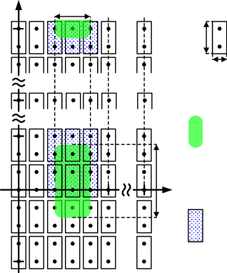
Figure 1: Illustration of the 2D block tiling $\{\mathcal{B}_{b}\}$, the effective support of a shifted leakage kernel $\Lambda_{p}^{(\theta)}[m,i]$, and the $\widetilde{N}_{\Lambda}$ blocks containing this effective support. In this example, $\Delta\widetilde{m}=2$, $\Delta\tilde{i}=4$, $\Delta m^{\prime}=1$, $\Delta i^{\prime}=2$, and $\widetilde{N}_{\Lambda}=9$.

IV-B Group Sparsity

We first analyze the group sparsity of $F_{m,i}^{(\theta)}$ for a single $\theta$. Consider a tiling of $\mathbb{Z}\times\mathbb{Z}$ into 2D blocks $\mathcal{B}_{b}$ of equal size $\Delta m^{\prime}\!\times\Delta i^{\prime}$, where $\Delta m^{\prime}$ divides $D$, $\Delta i^{\prime}$ divides $J/2$, and $[0,\Delta m^{\prime}\!-\!1]\times[0,\Delta i^{\prime}\!-\!1]$ is one of these blocks. As visualized in Fig. 1, the effective support of each shifted leakage kernel $\Lambda_{p}^{(\theta)}[m,i]$ within $[0,K\!-\!1]\times[0,L_{\textnormal{r}}-\!1]$ is contained in at most $\widetilde{N}_{\Lambda}$ blocks $\mathcal{B}_{b}$, where

$$\widetilde{N}_{\Lambda}\,\triangleq\hskip 0.85358pt\bigg{(}\bigg{\lceil}\frac{\Delta\widetilde{m}}{\Delta m^{\prime}}\bigg{\rceil}+1\bigg{)}\bigg{(}\bigg{\lceil}\frac{\Delta\tilde{i}}{\Delta i^{\prime}}\bigg{\rceil}+1\bigg{)}\hskip 0.85358pt.\vspace{-1.5mm}$$ (23)

Thus, by (21), the support of $S_{h}^{(\theta)}[m,i]$ is contained in at most $P\widetilde{N}_{\Lambda}$ blocks. Since $\Delta i^{\prime}$ divides $L$ (because $\Delta i^{\prime}$ divides $J/2$ and $J$ divides $L$), the summation in (19) only adds up whole blocks. Hence, the nonzeros contained in a single block are not spread over several blocks and thus no “new” nonzero blocks within the fundamental region $[0,D-1]\times[-J/2,J/2-1]$ are created. Also, since $\Delta m^{\prime}$ divides $D$ and $\Delta i^{\prime}$ divides $J/2$, the support restriction of $F_{m,i}^{(\theta)}$ to $[0,D\!-\!1]\times[-J/2,J/2\!-\!1]$ is compatible with the block boundaries. Thus, the effective support of $F_{m,i}^{(\theta)}$ within $[0,D-1]\times[-J/2,J/2-1]$ is contained in at most $P\widetilde{N}_{\Lambda}$ blocks. Therefore, $F_{m,i}^{(\theta)}$ is approximately group $P\widetilde{N}_{\Lambda}$-sparse with respect to the tiling $\{\mathcal{B}_{b}\}$.

IV-C Joint Sparsity

Next, we analyze the joint sparsity of the $F_{m,i}^{(\theta)}$, $\theta\in\Theta$. We first consider the shifted leakage kernels $\Lambda_{p}^{(\theta_{1})}[m,i]$ and $\Lambda_{p}^{(\theta_{2})}[m,i]$ of two different channels $\theta_{1}=(r_{1},s_{1})$ and $\theta_{2}=(r_{2},s_{2})$, corresponding to the same scatterer $p$. As mentioned in Section IV-A, these leakage kernels are effectively supported in rectangular regions of equal size $\Delta\widetilde{m}\times\Delta\tilde{i}$ that are centered about $\zeta_{p}^{(\theta_{1})}\!=\!\big{(}\tau_{p}^{(\theta_{1})}\!/\hskip 0.85358ptT_{{\text{s}}}\hskip 0.85358pt,\nu_{p}^{(\theta_{1})}T_{{\text{s}}}L_{\textnormal{r}}\big{)}$ and $\zeta_{p}^{(\theta_{2})}\!=\!\big{(}\tau_{p}^{(\theta_{2})}\!/\hskip 0.85358ptT_{{\text{s}}}\hskip 0.85358pt,\nu_{p}^{(\theta_{2})}T_{{\text{s}}}L_{\textnormal{r}}\big{)}$. We will show that, typically, these center points are very close to each other, and therefore the supports of the two leakage kernels strongly overlap.

Figure 2: Illustration of the propagation paths from the transmit antennas to the receive antennas via a scatterer $p$ in a $3\!\times\!3$ MIMO system.

IV-C1 Time delay

Consider the transmit antennas, the receive antennas, and some scatterer $p$, as shown in Fig. 2. Let $\mathbf{w}_{\textnormal{T},p}^{(s)}$ and $\mathbf{w}_{\textnormal{R},p}^{(r)}$ denote the vectors connecting scatterer $p$ with transmit antenna $s$ and receive antenna $r$, respectively, and let $w_{\textnormal{T},p}^{(s)}\triangleq\big{\|}\mathbf{w}_{\textnormal{T},p}^{(s)}\big{\|}_{2}$ and $w_{\textnormal{R},p}^{(r)}\triangleq\big{\|}\mathbf{w}_{\textnormal{R},p}^{(r)}\big{\|}_{2}$. The time delay $\tau_{p}^{(\theta)}$ for scatterer $p$ and antenna pair $\theta=(r,s)$ is then obtained as

$$\tau_{p}^{(\theta)}=\hskip 0.85358pt\frac{w_{\textnormal{T},p}^{(s)}+w_{\textnormal{R},p}^{(r)}}{c}\,,$$ (24)

where $c$ denotes the speed of light. We can bound the difference between the time delays of two channels $\theta_{1}$ and $\theta_{2}$, $\Delta\tau_{p}^{(\theta_{1},\theta_{2})}\triangleq\big{|}\tau_{p}^{(\theta_{1})}\!-\tau_{p}^{(\theta_{2})}\big{|}$, as

$$\Delta\tau_{p}^{(\theta_{1},\theta_{2})} =\hskip 0.85358pt\frac{1}{c}\hskip 0.85358pt\big{|}w_{\textnormal{T},p}^{(s_{1})}+w_{\textnormal{R},p}^{(r_{1})}-w_{\textnormal{T},p}^{(s_{2})}-w_{\textnormal{R},p}^{(r_{2})}\big{|}$$

$$\leq\hskip 0.85358pt\frac{1}{c}\hskip 0.85358pt\big{(}\big{|}w_{\textnormal{T},p}^{(s_{1})}-w_{\textnormal{T},p}^{(s_{2})}\big{|}+\big{|}w_{\textnormal{R},p}^{(r_{1})}-w_{\textnormal{R},p}^{(r_{2})}\big{|}\big{)}\,.$$ (25)

From geometric considerations, the difference between the transmitter-scatterer path lengths, $\big{|}w_{\textnormal{T},p}^{(s_{1})}-w_{\textnormal{T},p}^{(s_{2})}\big{|}$, cannot be larger than the distance between the two transmit antennas $s_{1}$ and $s_{2}$. This distance, in turn, is bounded by the maximum distance between any two transmit antennas, denoted by $d_{\textnormal{T}}$. Thus, $\big{|}w_{\textnormal{T},p}^{(s_{1})}-w_{\textnormal{T},p}^{(s_{2})}\big{|}\leq d_{\textnormal{T}}$. Using the same argument for the scatterer-receiver path, we obtain $\big{|}w_{\textnormal{R},p}^{(r_{1})}-w_{\textnormal{R},p}^{(r_{2})}\big{|}\leq d_{\textnormal{R}}$, where $d_{\textnormal{R}}$ denotes the maximum distance between any two receive antennas. Inserting these bounds into (25) gives

$$\Delta\tau_{p}^{(\theta_{1},\theta_{2})}\leq\tau_{\text{B}}\triangleq\frac{d_{\textnormal{T}}+d_{\textnormal{R}}}{c}\,.$$ (26)

IV-C2 Doppler frequency shift

Next, we consider the Doppler frequency shift $\nu_{p}^{(\theta)}$ for scatterer $p$ and antenna pair $\theta=(r,s)$. If the source of a sinusoidal wave with frequency $f_{\textnormal{0}}$ moves towards an observer with relative velocity $v$, at an angle $\alpha$ relative to the observer-source direction, the Doppler frequency shift is approximately $\nu=f_{\textnormal{0}}\frac{v}{c}\cos{\alpha}$ [65]. In our case, because transmitter, receiver, and scatterers are moving, the Doppler effect occurs twice. Let $\mathbf{v}_{\textnormal{T},p}$ and $\mathbf{v}_{\textnormal{R},p}$ denote the velocity vectors of scatterer $p$ relative to transmitter and receiver, respectively, and let $v_{\textnormal{T},p}\triangleq\left\lVert\mathbf{v}_{\textnormal{T},p}\right\rVert_{2}$ and $v_{\textnormal{R},p}\triangleq\left\lVert\mathbf{v}_{\textnormal{R},p}\right\rVert_{2}$. First, we consider the transmission from antenna $s$ to scatterer $p$, with carrier (center) frequency $f_{\textnormal{0}}$. Let $\alpha$ denote the angle between $\mathbf{v}_{\textnormal{T},p}$ and $\mathbf{w}_{\textnormal{T},p}^{(s)}$, and note that $\cos{\alpha}=\frac{\mathbf{v}_{\textnormal{T},p}^{T}\mathbf{w}_{\textnormal{T},p}^{(s)}}{v_{\textnormal{T},p}w_{\textnormal{T},p}^{(s)}}$. The carrier frequency observed at scatterer $p$ is approximately $f_{1}=f_{\textnormal{0}}+\nu_{\textnormal{T},p}^{(s)}\hskip 0.85358pt$, with

$$\nu_{\textnormal{T},p}^{(s)}\hskip 0.85358pt=\hskip 0.85358ptf_{\textnormal{0}}\hskip 0.85358pt\frac{v_{\textnormal{T},p}}{c}\hskip 0.85358pt\cos{\alpha}\,=\hskip 0.85358ptf_{\textnormal{0}}\hskip 0.85358pt\frac{v_{\textnormal{T},p}}{c}\hskip 0.85358pt\frac{\mathbf{v}_{\textnormal{T},p}^{T}\mathbf{w}_{\textnormal{T},p}^{(s)}}{v_{\textnormal{T},p}w_{\textnormal{T},p}^{(s)}}\hskip 0.85358pt=\hskip 0.85358pt\frac{f_{\textnormal{0}}}{c}\hskip 0.85358pt\frac{\mathbf{v}_{\textnormal{T},p}^{T}\mathbf{w}_{\textnormal{T},p}^{(s)}}{w_{\textnormal{T},p}^{(s)}}\,.$$ (27)

After transmission from scatterer $p$ to receive antenna $r$, the observed carrier frequency at receive antenna $r$ is given by $f_{2}=f_{1}+\nu_{\textnormal{R},p}^{(r)}\hskip 0.85358pt$, with the Doppler frequency shift (cf. (27))

$$\nu_{\textnormal{R},p}^{(r)}\hskip 0.85358pt=\hskip 0.85358pt\frac{f_{1}}{c}\hskip 0.85358pt\frac{\mathbf{v}_{\textnormal{R},p}^{T}\mathbf{w}_{\textnormal{R},p}^{(r)}}{w_{\textnormal{R},p}^{(r)}}\,.\vspace{-1.5mm}$$ (28)

Inserting for $f_{1}$ yields $f_{2}=f_{\textnormal{0}}+\nu_{\textnormal{T},p}^{(s)}+\nu_{\textnormal{R},p}^{(r)}$. Thus, the total Doppler frequency shift is

$$\nu_{p}^{(\theta)}=\hskip 0.85358pt\nu_{\textnormal{T},p}^{(s)}+\nu_{\textnormal{R},p}^{(r)}\,.$$ (29)

We can now bound the difference between the Doppler frequency shifts of two channels $\theta_{1}$ and $\theta_{2}$, $\Delta\nu_{p}^{(\theta_{1},\theta_{2})}\triangleq\big{|}\nu_{p}^{(\theta_{1})}\!-\nu_{p}^{(\theta_{2})}\big{|}$, as

$$\Delta\nu_{p}^{(\theta_{1},\theta_{2})} =\hskip 0.85358pt\big{|}\nu_{\textnormal{T},p}^{(s_{1})}+\nu_{\textnormal{R},p}^{(r_{1})}-\nu_{\textnormal{T},p}^{(s_{2})}-\nu_{\textnormal{R},p}^{(r_{2})}\big{|}$$

$$\leq\hskip 0.85358pt\big{|}\nu_{\textnormal{T},p}^{(s_{1})}-\nu_{\textnormal{T},p}^{(s_{2})}\big{|}+\big{|}\nu_{\textnormal{R},p}^{(r_{1})}-\nu_{\textnormal{R},p}^{(r_{2})}\big{|}\,.$$ (30)

For the transmitter-scatterer path, we obtain using (27)

$$\big{|}\nu_{\textnormal{T},p}^{(s_{1})}-\nu_{\textnormal{T},p}^{(s_{2})}\big{|} \,=\,\frac{f_{\textnormal{0}}}{c}\left|\mathbf{v}_{\textnormal{T},p}^{T}\!\left(\frac{\mathbf{w}_{\textnormal{T},p}^{(s_{1})}}{w_{\textnormal{T},p}^{(s_{1})}}-\frac{\mathbf{w}_{\textnormal{T},p}^{(s_{2})}}{w_{\textnormal{T},p}^{(s_{2})}}\right)\right|$$

$$\overset{(a)}{\leq}\hskip 0.85358pt\frac{f_{\textnormal{0}}}{c}\,v_{\textnormal{T},p}\,\Bigg{\|}\frac{\mathbf{w}_{\textnormal{T},p}^{(s_{1})}}{w_{\textnormal{T},p}^{(s_{1})}}-\frac{\mathbf{w}_{\textnormal{T},p}^{(s_{2})}}{w_{\textnormal{T},p}^{(s_{2})}}\Bigg{\|}_{2}$$

$$\overset{(b)}{\leq}\hskip 0.85358pt\frac{f_{\textnormal{0}}}{c}\,v_{\textnormal{T},p}\hskip 0.85358pt\frac{\big{\|}\mathbf{w}_{\textnormal{T},p}^{(s_{1})}-\mathbf{w}_{\textnormal{T},p}^{(s_{2})}\big{\|}_{2}}{w_{\textnormal{T},p,\textnormal{min}}^{(s_{1},s_{2})}}$$

$$\overset{(c)}{\leq}\hskip 0.85358pt\frac{f_{\textnormal{0}}}{c}\,\frac{v_{\textnormal{T},p}\hskip 0.85358ptd_{\textnormal{T}}}{w_{\textnormal{T},p,\textnormal{min}}^{(s_{1},s_{2})}}\,,$$

with $w_{\textnormal{T},p,\textnormal{min}}^{(s_{1},s_{2})}\triangleq\min\big{\{}w_{\textnormal{T},p}^{(s_{1})},w_{\textnormal{T},p}^{(s_{2})}\big{\}}$. Here, $(a)$ is due to the Cauchy-Schwarz inequality, $(b)$ follows from the inequality

$$\left\lVert\frac{\mathbf{a}}{{\|\mathbf{a}\|}_{2}}-\frac{\mathbf{b}}{{\|\mathbf{b}\|}_{2}}\right\rVert_{2}\hskip 0.85358pt\leq\,\frac{\left\lVert\mathbf{a}-\mathbf{b}\right\rVert_{2}}{\min\{\left\lVert\mathbf{a}\right\rVert_{2},\left\lVert\mathbf{b}\right\rVert_{2}\}}\;,$$ (31)

which is proven in Appendix A, and $(c)$ is a consequence of $\big{\|}\mathbf{w}_{\textnormal{T},p}^{(s_{1})}-\mathbf{w}_{\textnormal{T},p}^{(s_{2})}\big{\|}_{2}\leq d_{\textnormal{T}}$. A similar derivation for the scatterer-receiver path, using (28), yields $\big{|}\nu_{\textnormal{R},p}^{(r_{1})}-\nu_{\textnormal{R},p}^{(r_{2})}\big{|}\leq\frac{f_{1}}{c}\hskip 0.85358pt\frac{v_{\textnormal{R},p}\hskip 0.85358ptd_{\textnormal{R}}}{w_{\textnormal{R},p,\textnormal{min}}^{(r_{1},r_{2})}}$, where $w_{\textnormal{R},p,\textnormal{min}}^{(r_{1},r_{2})}\triangleq\min\big{\{}w_{\textnormal{R},p}^{(r_{1})},w_{\textnormal{R},p}^{(r_{2})}\big{\}}$. Inserting these bounds into (30), we obtain

$$\Delta\nu_{p}^{(\theta_{1},\theta_{2})}\leq\hskip 0.85358pt\nu_{\text{B},p}^{(\theta_{1},\theta_{2})}\triangleq\hskip 0.85358pt\frac{1}{c}\!\left(\frac{f_{\textnormal{0}}\hskip 0.85358ptv_{\textnormal{T},p}\hskip 0.85358ptd_{\textnormal{T}}}{w_{\textnormal{T},p,\textnormal{min}}^{(s_{1},s_{2})}}+\frac{f_{1}v_{\textnormal{R},p}\hskip 0.85358ptd_{\textnormal{R}}}{w_{\textnormal{R},p,\textnormal{min}}^{(r_{1},r_{2})}}\right).$$ (32)

IV-C3 Joint sparsity of the $F_{m,i}^{(\theta)}$

From (26) and (32), it follows that the center points $\zeta_{p}^{(\theta_{1})}\!=\!\big{(}\tau_{p}^{(\theta_{1})}\!/\hskip 0.85358ptT_{{\text{s}}}\hskip 0.85358pt,\nu_{p}^{(\theta_{1})}T_{{\text{s}}}L_{\textnormal{r}}\big{)}$ and $\zeta_{p}^{(\theta_{2})}\!=\!\big{(}\tau_{p}^{(\theta_{2})}\!/\hskip 0.85358ptT_{{\text{s}}}\hskip 0.85358pt,\nu_{p}^{(\theta_{2})}T_{{\text{s}}}L_{\textnormal{r}}\big{)}$ of $\Lambda_{p}^{(\theta_{1})}[m,i]$ and $\Lambda_{p}^{(\theta_{2})}[m,i]$ differ by at most $\tau_{\text{B}}/T_{{\text{s}}}$ in the $m$-direction and by at most $\nu_{\text{B},p}^{(\theta_{1},\theta_{2})}\hskip 0.85358ptT_{{\text{s}}}L_{\textnormal{r}}$ in the $i$-direction. Since this holds for any pair of channels $\theta_{1}$ and $\theta_{2}$, we conclude that all $\Lambda_{p}^{(\theta)}[m,i]$, $\theta\in\Theta$ are (approximately) jointly $\Delta m\hskip 0.85358pt\Delta i$-sparse, where

$$\Delta m\,\triangleq\,\Delta\widetilde{m}+\lceil\tau_{\text{B}}/T_{{\text{s}}}\rceil\quad\;\text{and}\quad\;\Delta i\,\triangleq\,\Delta\tilde{i}+\lceil\nu_{\text{B}}\hskip 0.85358ptT_{{\text{s}}}L_{\textnormal{r}}\rceil\,,$$

with $\nu_{\text{B}}\triangleq\max_{p,\hskip 0.85358pt\theta_{1}\neq\theta_{2}}\!\big{\{}\nu_{\text{B},p}^{(\theta_{1},\theta_{2})}\big{\}}$. (Here, we used the fact that the effective supports of $\Lambda_{p}^{(\theta_{1})}[m,i]$ and $\Lambda_{p}^{(\theta_{2})}[m,i]$ have size $\Delta\widetilde{m}\times\Delta\tilde{i}$.) With (21), it then follows that the spreading functions $S_{h}^{(\theta)}[m,i]$ are (approximately) jointly $P\Delta m\hskip 0.85358pt\Delta i$-sparse. Finally, because of (19), the same is true for the $F_{m,i}^{(\theta)}$ (as discussed before).

Since the antenna spacings are typically much smaller than the path lengths, i.e., $d_{\textnormal{T}}\ll w_{\textnormal{T},p}^{(s)}$ and $d_{\textnormal{R}}\ll w_{\textnormal{R},p}^{(r)}\hskip 0.85358pt$, and for practical velocities $v_{\textnormal{T},p}$ and $v_{\textnormal{R},p}\hskip 0.85358pt$, $\lceil\tau_{\text{B}}/T_{{\text{s}}}\rceil$ and $\lceil\nu_{\text{B}}\hskip 0.85358ptT_{{\text{s}}}L_{\textnormal{r}}\rceil$ will be small compared to $\Delta\widetilde{m}$ and $\Delta\tilde{i}$, respectively. Therefore, the joint sparsity order $P\Delta m\hskip 0.85358pt\Delta i=P\hskip 0.85358pt\big{(}\Delta\widetilde{m}+\lceil\tau_{\text{B}}/T_{{\text{s}}}\rceil\big{)}\hskip 0.85358pt\big{(}\Delta\tilde{i}+\lceil\nu_{\text{B}}\hskip 0.85358ptT_{{\text{s}}}L_{\textnormal{r}}\rceil\big{)}$ will not be much larger than the individual sparsity orders $P\Delta\widetilde{m}\hskip 0.85358pt\Delta\tilde{i}$ of the $F_{m,i}^{(\theta)}$.

IV-D Joint Group Sparsity

We reconsider the tiling of $\mathbb{Z}\times\mathbb{Z}$ into the 2D blocks $\mathcal{B}_{b}$ as previously considered in Section IV-B, restricting it to $[0,D\!-\!1]\times[-J/2,J/2\!-\!1]$ (see Fig. 1). Within that region, we obtain a finite number $B$ of blocks $\mathcal{B}_{b}$, $b\in\{1,\dots,B\}$. We recall that the blocks are of equal size $|\mathcal{B}_{b}|=\Delta m^{\prime}\Delta i^{\prime}$, and hence $B=\frac{JD}{\Delta m^{\prime}\Delta i^{\prime}}$. Since the leakage kernels $\Lambda_{p}^{(\theta)}[m,i]$, $\theta\in\Theta$ are (approximately) jointly $\Delta m\hskip 0.85358pt\Delta i$-sparse, as we just showed in Section IV-C, it follows by the same reasoning as in Section IV-B that their effective supports are jointly contained in at most $N_{\Lambda}$ blocks $\mathcal{B}_{b}$, where (cf. (23))

$$N_{\Lambda}\,\triangleq\hskip 0.85358pt\bigg{(}\bigg{\lceil}\frac{\Delta m}{\Delta m^{\prime}}\bigg{\rceil}+1\bigg{)}\bigg{(}\bigg{\lceil}\frac{\Delta i}{\Delta i^{\prime}}\bigg{\rceil}+1\bigg{)}\hskip 0.85358pt.\vspace{-1mm}$$

Thus, again because of (21) and (19), the $F_{m,i}^{(\theta)}\hskip 0.85358pt$, $\theta\in\Theta$ are (approximately) jointly group $PN_{\Lambda}$-sparse with respect to the tiling ${\{\mathcal{B}_{b}\}}_{b=1}^{B}$.

This joint group sparsity of the $F_{m,i}^{(\theta)}$ translates into a joint group sparsity of the vectors $\operatorname{{rvec}}_{m,i}\big{\{}F_{m,i}^{(\theta)}\big{\}}$, $\theta\in\Theta$ defined in Section IV-A. The stacking operator $\operatorname{{rvec}}_{m,i}\{\cdot\}$ corresponds to the one-to-one 2D $\to$ 1D index mapping $\mathsf{S}\!:\{0,\dots,D\!-\!1\}\times\{-J/2,\dots,J/2\!-\!1\}\rightarrow\{1,\dots,JD\}$ given by

$$\mathsf{S}(m,i)\,\triangleq\,mJ+i+\frac{J}{2}+1\hskip 0.85358pt.$$ (33)

Under this index mapping, the 2D blocks $\mathcal{B}_{b}$ are converted into the 1D groups $\mathcal{I}_{b}\triangleq\mathsf{S}(\mathcal{B}_{b})\subseteq\{1,\dots,JD\}$, $b\in\{1,\dots,B\}$, which are of equal size $|\mathcal{I}_{b}|=|\mathcal{B}_{b}|=\Delta m^{\prime}\Delta i^{\prime}$. Clearly, $\mathcal{J}\triangleq{\{\mathcal{I}_{b}\}}_{b=1}^{B}$ constitutes a partition of $\{1,\dots,JD\}$, as required by the definition of joint group sparsity in Section III-C. Then, because the effective supports of all the $F^{(\theta)}_{m,i}$ within $\{0,\dots,D\!-\!1\}\times\{-J/2,\dots,J/2\!-\!1\}$ are jointly contained in at most $PN_{\Lambda}$ blocks $\mathcal{B}_{b}$, it follows that the vectors $\operatorname{{rvec}}_{m,i}\big{\{}F_{m,i}^{(\theta)}\big{\}}$ are (approximately) jointly group $PN_{\Lambda}$-sparse with respect to the 1D partition $\mathcal{J}$.

V Compressive MIMO Channel Estimation
Exploiting Joint Group Sparsity

The MGCS-based MC-MIMO channel estimator presented in this section exploits the joint group sparsity of doubly selective MC-MIMO channels studied in Section IV. It generalizes the estimators previously presented in [17, 32, 29].

V-A Subsampled Time-Frequency Grid and Pilot Arrangement

As in Section IV, we assume that the support of $\mathbf{F}_{m,i}$ is contained in $[0,D\!-\!1]\times[-J/2,J/2\!-\!1]$. By the 2D discrete Fourier transform (DFT) relation in (8), the channel coefficient matrices $\mathbf{H}_{l,k}$ are then uniquely determined by their values on the subsampled time-frequency grid

$$\mathcal{G} \hskip 0.85358pt\triangleq\hskip 0.85358pt\big{\{}(l,k)=(\lambda\,\Delta L,\kappa\,\Delta K)\,\big{|}\,\lambda\in\{0,\dots,J\!-\!1\},$$

$$\hskip 142.26378pt\kappa\in\{0,\dots,D\!-\!1\}\big{\}}\,.$$

Due to (8), these subsampled values are given by

$$\mathbf{H}_{\lambda\,\Delta L,\kappa\,\Delta K}\,=\,\sum_{m=0}^{D-1}\sum_{i=-J/2}^{J/2-1}\!\!\mathbf{F}_{m,i}\,e^{-j2\pi(\frac{\kappa m}{D}-\frac{\lambda i}{J})},\vspace{-.5mm}$$ (34)

with jointly group sparse coefficient matrices $\mathbf{F}_{m,i}$ (cf. Section IV). However, the sparsity is impaired by leakage effects. To reduce them and, thereby, improve the joint group sparsity of $\mathbf{F}_{m,i}$, we generalize (34) to an orthonormal 2D basis expansion

$$\mathbf{H}_{\lambda\,\Delta L,\kappa\,\Delta K}\,=\,\sum_{m=0}^{D-1}\sum_{i=-J/2}^{J/2-1}\!\!\mathbf{G}_{m,i}\,u_{m,i}[\lambda,\kappa]\,,\vspace{-.5mm}$$ (35)

with some orthonormal 2D basis $\{u_{m,i}[\lambda,\kappa]\}$. The construction of a basis yielding improved joint group sparsity of the $G_{m,i}^{(\theta)}\triangleq{[\mathbf{G}_{m,i}]}_{r,s}$ (recall that $\theta\!=\!(r,s)$) will be studied in Section VI. Clearly, the 2D DFT (34) is a special case of (35) with $\mathbf{G}_{m,i}=\sqrt{JD}\,\mathbf{F}_{m,i}$ and $u_{m,i}[\lambda,\kappa]=\frac{1}{\sqrt{JD}}\,e^{-j2\pi(\frac{\kappa m}{D}-\frac{\lambda i}{J})}$.

Let $\mu\triangleq(l,k)$ index the (nonsubsampled) time-frequency positions. For pilot-aided channel estimation, we choose $N_{\text{T}}$ linearly independent pilot vectors $\mathbf{p}^{(s)}\!\triangleq\big{(}p_{1}^{(s)}\cdots\hskip 0.85358ptp_{N_{\text{T}}}^{(s)}\big{)}^{T}\!$, $s\in$$\{1,\dots,N_{\text{T}}\}$ and $N_{\text{T}}$ pairwise disjoint sets of pilot time-frequency positions $\mathcal{P}^{(s)}\!$, $s\in\{1,\dots,N_{\text{T}}\}$. The $\mathcal{P}^{(s)}$ are subsets of the subsampled time-frequency grid $\mathcal{G}$, i.e., $\mathcal{P}^{(s)}\!\subseteq\mathcal{G}$, with equal size $Q\triangleq|\mathcal{P}^{(s)}|$. Let $\mu_{q}^{(s)}\!$, $q\in\{1,\dots,Q\}$ denote the pilot time-frequency positions in $\mathcal{P}^{(s)}\!$. For each $s\in\{1,$$\dots,N_{\text{T}}\}$, the pilot vector $\mathbf{p}^{(s)}$ is transmitted at all $Q$ time-frequency positions $\mu_{q}^{(s)}\!\in\!\mathcal{P}^{(s)}\!$, i.e., $\mathbf{a}_{\mu_{q}^{(s)}}\!=\!\mathbf{p}^{(s)}$ for all $q\in\{1,$$\dots,Q\}$ in (1). Thus, $N_{\text{T}}Q$ pilot vectors, or $N_{\text{T}}^{2}Q$ pilots symbols, are transmitted in total. An example of such a pilot arrangement is shown in Fig. 3. Note that the individual entries of $\mathbf{a}_{\mu_{q}^{(s)}}\!=\!\mathbf{p}^{(s)}$ correspond to pilots at the same time-frequency position, but transmitted from different antennas.

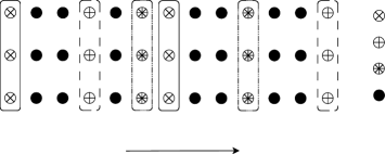
Figure 3: Example of a pilot arrangement for $N_{\text{T}}=3$ transmit antennas. For each $s\in\{1,2,3\}$, the same length-$3$ pilot vector $\mathbf{p}^{(s)}$ is transmitted at all time-frequency positions $(l,k)\in\mathcal{P}^{(s)}$. Note that $Q=|\mathcal{P}^{(s)}|=2$.

V-B The Estimator

Let $y^{(r)}_{\mu}\!\triangleq{[\mathbf{y}_{\mu}]}_{r}$ (cf. (3)) denote the demodulated symbol at receive antenna $r$ and time-frequency position $\mu$, with $z^{(r)}_{\mu}\!\triangleq{[\mathbf{z}_{\mu}]}_{r}$ (cf. (5)) the associated noise component. Furthermore let

$$\tilde{G}_{m,i}^{(\theta)}\hskip 0.85358pt\triangleq\,\mathbf{g}^{(r)T}_{m,i}\mathbf{p}^{(s)},\vspace{-1mm}$$ (36)

where $\mathbf{g}^{(r)T}_{m,i}\!$ denotes the $r\hskip 0.85358pt$th row of $\mathbf{G}_{m,i}$. Then, writing $\mu_{q}^{(s)}\triangleq(\lambda_{q}^{(s)}\Delta L,\kappa_{q}^{(s)}\Delta K)$ for the pilot time-frequency positions and using (5), (35), and (36), we obtain

$$y^{(r)}_{\mu_{q}^{(s)}} \,=\,{\big{[}\mathbf{y}_{\!\mu_{q}^{(s)}}\big{]}}_{r}$$

$$\hskip 0.85358pt\overset{(\ref{gen.io.rel})}{=}\,{\big{[}\mathbf{H}_{\mu_{q}^{(s)}}\mathbf{p}^{(s)}+\mathbf{z}_{\mu_{q}^{(s)}}\big{]}}_{r}$$

$$\overset{(\ref{Gen_Basis_Exp})}{=}\Bigg{[}\Bigg{(}\sum_{m=0}^{D-1}\sum_{i=-J/2}^{J/2-1}\!\mathbf{G}_{m,i}\,u_{m,i}\big{[}\lambda_{q}^{(s)},\kappa_{q}^{(s)}\big{]}\Bigg{)}\hskip 0.85358pt\mathbf{p}^{(s)}+\mathbf{z}_{\mu_{q}^{(s)}}\Bigg{]}_{r}$$

$$\,=\,\sum_{m=0}^{D-1}\sum_{i=-J/2}^{J/2-1}\!\mathbf{g}_{m,i}^{(r)T}\mathbf{p}^{(s)}\hskip 0.85358ptu_{m,i}\big{[}\lambda_{q}^{(s)},\kappa_{q}^{(s)}\big{]}\hskip 0.85358pt+\hskip 0.85358ptz_{\mu_{q}^{(s)}}^{(r)}$$

$$\overset{(\ref{eq_G-k})}{=}\sum_{m=0}^{D-1}\sum_{i=-J/2}^{J/2-1}\!\tilde{G}_{m,i}^{(\theta)}\,u_{m,i}\big{[}\lambda_{q}^{(s)},\kappa_{q}^{(s)}\big{]}\,+\,z^{(r)}_{\mu_{q}^{(s)}}\,,$$ (37)

for all $q\in\{1,\dots,Q\}$, $s\in\{1,\dots,N_{\text{T}}\}$, and $r\in\{1,\dots,N_{\text{R}}\}$. To rewrite this relation in vector-matrix notation, we define $\mathbf{U}$ to be the unitary $JD\times\!JD$ matrix whose $(mJ+i+J/2+1)\hskip 0.85358pt$th column is given by $\operatorname{{rvec}}_{\lambda,\kappa}\big{\{}u_{m,i}[\lambda,\kappa]\big{\}}=\big{(}u_{m,i}[0,0]$$u_{m,i}[0,1]\,\cdots\,u_{m,i}[1,0]\,\cdots\,u_{m,i}[J\!-\!1,D\!-\!1]\big{)}^{T}\!$ (this denotes the rowwise stacking with respect to $\lambda,\kappa$ of the $J\!\times\!D$ “matrix” $u_{m,i}[\lambda,\kappa]$ into a $JD$-dimensional vector). Furthermore, we set

$$\mathbf{\Phi}^{(s)}\triangleq\hskip 0.85358pt\sqrt{\frac{JD}{Q}}\,\mathbf{U}^{(s)}\in\hskip 0.85358pt\mathbb{C}^{Q\times JD},\vspace{.5mm}$$ (38)

where $\mathbf{U}^{(s)}$ denotes the $Q\!\times\!JD$ submatrix of $\mathbf{U}$ constituted by the $Q$ rows corresponding to the pilot positions $\mu_{q}^{(s)}\!\in\mathcal{P}^{(s)}$, $q\in\{1,\dots,Q\}$. We also define the vectors

$$\mathbf{x}^{(\theta)}\,\triangleq\,\sqrt{\frac{Q}{JD}}\,\operatorname{{rvec}}_{m,i}\big{\{}\tilde{G}_{m,i}^{(\theta)}\big{\}}\in\hskip 0.85358pt\mathbb{C}^{JD},$$ (39)

as well as the vectors $\mathbf{y}^{(\theta)}\triangleq\big{(}y^{(\theta)}_{1}\cdots\hskip 0.85358pty^{(\theta)}_{Q}\big{)}^{T}\!\!\in\mathbb{C}^{Q}$ with $y^{(\theta)}_{q}\!\triangleq y^{(r)}_{\mu_{q}^{(s)}}$ and $\mathbf{z}^{(\theta)}\!\triangleq\big{(}z^{(\theta)}_{1}\cdots\hskip 0.85358ptz^{(\theta)}_{Q}\big{)}^{T}\!\!\in\mathbb{C}^{Q}$ with $z^{(\theta)}_{q}\triangleq z^{(r)}_{\mu_{q}^{(s)}}$. We can then rewrite (37) as

$$\mathbf{y}^{(\theta)}=\hskip 0.85358pt\mathbf{\Phi}^{(s)}\mathbf{x}^{(\theta)}+\mathbf{z}^{(\theta)},\quad\theta=(r,s)\in\Theta\hskip 0.85358pt.\vspace{-.5mm}$$ (40)

Thus, we obtained measurement equations of the form (14), of dimension $Q\times\!JD$ (i.e., $M=JD$). In practice, $Q\ll\!JD$. Since the coefficients $G_{m,i}^{(\theta)}$ are (approximately) jointly group sparse, the functions $\tilde{G}_{m,i}^{(\theta)}=\mathbf{g}^{(r)T}_{m,i}\mathbf{p}^{(s)}$ and, consequently, the vectors $\mathbf{x}^{(\theta)}$ are (approximately) jointly group sparse as well. Therefore, (40) is recognized as an instance of the MGCS problem introduced in Section III-C, and thus any MGCS reconstruction method can be used to reconstruct the $\mathbf{x}^{(\theta)}$.

We can now state the overall channel estimation algorithm:

1. Stack the demodulated symbols at the pilot positions, $y^{(r)}_{\mu_{q}^{(s)}}$, into vectors $\mathbf{y}^{(\theta)}$ (see above) and obtain estimates $\hat{\mathbf{x}}^{(\theta)}$ of the $\mathbf{x}^{(\theta)}$ via an MGCS reconstruction method based on the measurement matrices $\mathbf{\Phi}^{(s)}\!$.

2. Rescale these estimates $\hat{\mathbf{x}}^{(\theta)}$ with $\sqrt{JD/Q}$ to obtain estimates $\hat{\tilde{G}}_{m,i}^{(\theta)}$ of $\tilde{G}_{m,i}^{(\theta)}$, i.e., calculate $\operatorname{{rvec}}_{m,i}\{\hat{\tilde{G}}_{m,i}^{(\theta)}\}=\sqrt{JD/Q}\,\hat{\mathbf{x}}^{(\theta)}$ (cf. the definition of $\mathbf{x}^{(\theta)}$ in (39)).

3. Calculate (cf. (36))

   $$\hat{\mathbf{g}}^{(r)}_{m,i}\hskip 0.85358pt=\hskip 0.85358pt\mathbf{P}^{-T}\big{(}\hat{\tilde{G}}_{m,i}^{(r,1)}\cdots\,\hat{\tilde{G}}_{m,i}^{(r,N_{\text{T}})}\big{)}^{T}\vspace{-.5mm}$$

   with $\mathbf{P}\triangleq\big{(}\mathbf{p}^{(1)}\cdots\hskip 0.85358pt\mathbf{p}^{(N_{\text{T}})}\big{)}$. Note that $\mathbf{P}$ is nonsingular as the $\mathbf{p}^{(s)}$ were chosen linearly independent.

4. From $\hat{\mathbf{g}}^{(r)}_{m,i}$, calculate estimates $\hat{\mathbf{H}}_{\lambda\,\Delta L,\kappa\,\Delta K}$ of the subsampled channel coefficient matrices $\mathbf{H}_{\lambda\,\Delta L,\kappa\,\Delta K}$ according to (35) with $\mathbf{G}_{m,i}$ replaced by $\hat{\mathbf{G}}_{m,i}$.

5. Calculate estimates of the 2D DFT coefficients $\mathbf{F}_{m,i}$ according to the inversion of (34), i.e.,

   $$\hat{\mathbf{F}}_{m,i}\hskip 0.85358pt=\hskip 0.85358pt\frac{1}{JD}\sum_{\lambda=0}^{J-1}\sum_{\kappa=0}^{D-1}\hat{\mathbf{H}}_{\lambda\,\Delta L,\kappa\,\Delta K}\,e^{-j2\pi(\frac{i\lambda}{J}-\frac{m\kappa}{D})}\vspace{-1mm}$$ (41)

   for $m\in\{0,\dots,D\!-\!1\}$ and $i\in\{-J/2,\dots,J/2\!-\!1\}$. Set $\hat{\mathbf{F}}_{m,i}=\mathbf{0}$ otherwise.

6. Calculate estimates $\hat{\mathbf{H}}_{l,k}$ of all $\mathbf{H}_{l,k}$ by using the 2D DFT expansion (8) with $\mathbf{F}_{m,i}$ replaced by $\hat{\mathbf{F}}_{m,i}$.

In the special case where the 2D DFT basis is used, steps 4 and 5 can be omitted because $\mathbf{F}_{m,i}=\mathbf{G}_{m,i}/\sqrt{JD}$.

According to their definition in (38), the measurement matrices $\mathbf{\Phi}^{(s)}$ are constructed by selecting those $|\mathcal{P}^{(s)}|\!=\!Q$ rows of the scaled unitary matrix $\sqrt{JD/Q}\,\mathbf{U}$ that correspond to the pilot positions $\mu_{q}^{(s)}\!\in\mathcal{P}^{(s)}\!$. Therefore, motivated by the construction of measurement matrices described in Section III-A, we choose these rows—or, in other words, the pilot positions $\mu_{q}^{(s)}$—uniformly at random from the subsampled grid $\mathcal{G}$. More precisely, we first choose a subset of $\mathcal{G}$ of size $N_{\text{T}}Q$ uniformly at random, and then we partition it into $N_{\text{T}}$ pairwise disjoint sets $\mathcal{P}^{(s)}\!$, $s\in\{1,\dots,N_{\text{T}}\}$ of equal size $Q$. This construction differs from the construction of measurement matrices explained in Section III-A in that here the pilot sets $\mathcal{P}^{(s)}$ (i.e. the rows of the unitary matrix $\sqrt{JD/Q}\,\mathbf{U}$) have to be chosen pairwise disjoint, which contradicts the assumption underlying (13) that each row of $\sqrt{JD/Q}\,\mathbf{U}$ be chosen with equal probability. Unfortunately, an analysis of the G-RIC for this exact scenario does not seem to exist. Nevertheless, we can expect $\mathbf{\Phi}^{(s)}$ to satisfy the group restricted isometry property with a small G-RIC with high probability (as explained in Section III-A) if the pilot sets are chosen sufficiently large. We also note that CS channel estimation methods have been shown to be robust to the choice of the pilot pattern [66].

The pilot positions are chosen in a design phase before the start of data transmission and then remain fixed. Therefore, once pilot sets $\mathcal{P}^{(s)}$ yielding matrices $\mathbf{\Phi}^{(s)}$ with “good” MGCS reconstruction properties are found, they can be used for all future data transmissions.

V-C Performance Analysis

We next present upper bounds on the estimation error of our channel estimator. Let $\mathcal{J}={\{\mathcal{I}_{b}\}}_{b=1}^{B}$ be the partition used by the MGCS reconstruction method in step $1$, let $\mathcal{S}\subseteq\{1,\ldots,$$B\}$ comprise the indices $b$ of those $S$ groups $\mathcal{I}_{b}$ that contain the effective joint support of the vectors $\operatorname{{rvec}}_{m,i}\big{\{}G_{m,i}^{(\theta)}\big{\}}$, and let $\big{(}\operatorname{{rvec}}_{m,i}\big{\{}G_{m,i}^{(\theta)}\big{\}}\big{)}[b]\in\mathbb{C}^{|\mathcal{I}_{b}|}$ be composed of those entries of $\operatorname{{rvec}}_{m,i}\big{\{}G_{m,i}^{(\theta)}\big{\}}$ whose indices are in $\mathcal{I}_{b}$. Then, the leakage of the vectors $\operatorname{{rvec}}_{m,i}\big{\{}G_{m,i}^{(\theta)}\big{\}}$ outside $\mathcal{S}$ and, thus, the error of a joint group $S$-sparsity assumption (i.e., the error incurred when the entries of the vectors $\operatorname{{rvec}}_{m,i}\big{\{}G_{m,i}^{(\theta)}\big{\}}$ outside these $S$ groups are set to zero) can be quantified by

$$C_{G,\mathcal{S},\mathcal{J}}\hskip 0.85358pt\triangleq\,\sum_{b\hskip 0.85358pt\notin\mathcal{S}}\bigg{(}\sum_{\theta\in\Theta}\big{\|}\big{(}\operatorname{{rvec}}_{m,i}\big{\{}G_{m,i}^{(\theta)}\big{\}}\big{)}[b]\big{\|}_{2}^{2}\bigg{)}^{\!1/2}.$$ (42)

We also define the root mean square error (RMSE) of channel estimation

$$E\,\triangleq\hskip 0.85358pt\Bigg{(}\sum_{\theta\in\Theta}\sum_{l=0}^{L-1}\sum_{k=0}^{K-1}\big{|}\hat{H}^{(\theta)}_{l,k}-H^{(\theta)}_{l,k}\big{|}^{2}\Bigg{)}^{\!1/2},$$ (43)

with $H^{(\theta)}_{l,k}\triangleq{[\mathbf{H}_{l,k}]}_{r,s}$ and $\hat{H}^{(\theta)}_{l,k}\triangleq{[\hat{\mathbf{H}}_{l,k}]}_{r,s}$. In the following theorem, we consider the MGCS-based channel estimator described in Section V-B, where the MGCS reconstruction method in step $1$ is G-BPDN or G-CoSaMP (see Section III-A) operating in the MGCS mode (see Section III-C), so that joint and group sparsity are leveraged simultaneously. The proof of the theorem is given in Appendix B.

Theorem 1

Assume that the noise $\mathbf{z}^{(\theta)}$ in (40) satisfies $\big{(}\sum_{\theta\in\Theta}{\|\mathbf{z}^{(\theta)}\|}_{2}^{2}\big{)}^{1/2}\leq\epsilon$ for some $\epsilon>0$. First, let the MGCS reconstruction method in step 1 be G-BPDN operating in MGCS mode. If all $\mathbf{\Phi}^{(s)}$ in (40) satisfy the group restricted isometry property of order $2S$ with respect to $\mathcal{J}$ with G-RIC $\delta_{2S|\mathcal{J}}^{(s)}\leq\sqrt{2}-1$, then

$$E\hskip 0.85358pt\leq\,C_{0}^{\prime}\frac{C_{G,\mathcal{S},\mathcal{J}}}{\sqrt{S}}+C_{1}^{\prime}\epsilon\,,\vspace{-1.5mm}$$ (44)

with the constants $C_{0}^{\prime}\triangleq c_{0}\sqrt{KL/(JD)}\,\|\mathbf{P}\|\hskip 0.85358pt\|\mathbf{P}^{-1}\|$ and $C_{1}^{\prime}\triangleq c_{1}\sqrt{KL/Q}\hskip 0.85358pt\|\mathbf{P}^{-1}\|$, where $c_{0}=\frac{2\hskip 0.85358pt(1\hskip 0.85358pt-\hskip 0.85358pt\delta_{2S|\mathcal{J}})}{1\hskip 0.85358pt-\hskip 0.85358pt(1\hskip 0.85358pt+\hskip 0.85358pt\sqrt{2})\hskip 0.85358pt\delta_{2S|\mathcal{J}}}$, $c_{1}=\frac{4\hskip 0.85358pt\sqrt{1\hskip 0.85358pt+\hskip 0.85358pt\delta_{2S|\mathcal{J}}}}{1\hskip 0.85358pt-\hskip 0.85358pt(1\hskip 0.85358pt+\hskip 0.85358pt\sqrt{2})\hskip 0.85358pt\delta_{2S|\mathcal{J}}}$, and $\left\lVert\cdot\right\rVert$ denotes the spectral norm [67]. Alternatively, assume that step 1 uses G-CoSaMP with $n$ iterations operating in MGCS mode. If all $\mathbf{\Phi}^{(s)}$ satisfy the group restricted isometry property of order $4S$ with respect to $\mathcal{J}$ with G-RIC $\delta_{4S|\mathcal{J}}^{(s)}\leq 0.1$, then

$$E\hskip 0.85358pt\leq\,C_{0}^{\prime\prime}\Big{(}1+\frac{1}{\sqrt{S}}\Big{)}\hskip 0.85358ptC_{G,\mathcal{S},\mathcal{J}}+\hskip 0.85358ptC_{1}^{\prime\prime}\epsilon\hskip 0.85358pt+\hskip 0.85358ptC_{2}^{\prime\prime}(n)\,,\vspace{-1.5mm}$$ (45)

with the constants $C_{0}^{\prime\prime}\triangleq 20\hskip 0.85358pt\sqrt{KL/(JD)}\,\|\mathbf{P}\|\hskip 0.85358pt\|\mathbf{P}^{-1}\|$, $C_{1}^{\prime\prime}\triangleq 20\hskip 0.85358pt\sqrt{KL/Q}\hskip 0.85358pt\|\mathbf{P}^{-1}\|$, and $C_{2}^{\prime\prime}(n)\triangleq 2^{-n}\hskip 0.85358pt\|\mathbf{P}\|\hskip 0.85358pt\|\mathbf{P}^{-1}\|\hskip 0.85358pt\big{(}KL/(JD)$$\times\sum_{\theta\in\Theta}\sum_{m=0}^{D-1}\sum_{i=-J/2}^{J/2-1}\big{|}G_{m,i}^{(\theta)}\big{|}^{2}\big{)}^{1/2}$.

Note that $C_{2}^{\prime\prime}(n)$ can be made arbitrarily small by increasing the number $n$ of G-CoSaMP iterations. Furthermore, as mentioned at the end of Section V-B, the $\mathbf{\Phi}^{(s)}$ can be expected to satisfy the group restricted isometry property with sufficiently small G-RICs $\delta_{2S|\mathcal{J}}^{(s)}$ and $\delta_{4S|\mathcal{J}}^{(s)}$ (with high probability) if the size of the pilot sets $\mathcal{P}^{(s)}$ is sufficiently large. Finally, while the bounds (44) and (45) are pessimistic in general, i.e., the actual estimation accuracy is typically much better, they express the dependence on various system parameters and can therefore provide valuable design guidelines.

V-D Computational Complexity

To analyze the complexity of the proposed method, we consider each step individually. The complexity of step 1 depends on the MGCS algorithm used and will be denoted as $\mathcal{O}(\text{MGCS})$. The rescaling performed in step 2 requires $\mathcal{O}\big{(}N_{\text{T}}N_{\text{R}}JD\big{)}$ operations. The complexity of step 3 is $\mathcal{O}\big{(}N_{\text{T}}^{2}N_{\text{R}}JD\big{)}$, because $\mathbf{P}^{-T}$ is of size $N_{\text{T}}\times N_{\text{T}}$, and thus each of the $N_{\text{R}}$ matrix-vector products has complexity $\mathcal{O}\big{(}N_{\text{T}}^{2}\big{)}$ (note that $\mathbf{P}$ has to be inverted only once before the start of data transmission). Evaluating (35) in step 4 in an entrywise (i.e., channel-by-channel) fashion requires $\mathcal{O}\big{(}N_{\text{T}}N_{\text{R}}(JD)^{2}\big{)}$ operations; a more efficient computation of (35) may be possible if the matrix $\mathbf{U}$ with columns $\operatorname{{rvec}}_{\lambda,\kappa}\big{\{}u_{m,i}[\lambda,\kappa]\big{\}}$ has a suitable structure. In step 5, again proceeding entrywise, the calculation of (41) can be performed efficiently in $\mathcal{O}\big{(}N_{\text{T}}N_{\text{R}}JD\log(JD)\big{)}$ operations by using the FFT. By the same reasoning, step 6 has complexity $\mathcal{O}\big{(}N_{\text{T}}N_{\text{R}}KL\log(KL)\big{)}$. Therefore, the overall complexity of the proposed channel estimator is obtained as

$$\mathcal{O}(\text{MGCS})+\hskip 0.85358pt\mathcal{O}\big{(}N_{\text{T}}N_{\text{R}}\hskip 0.85358pt(JD)^{2}\big{)}+\hskip 0.85358pt\mathcal{O}\big{(}N_{\text{T}}N_{\text{R}}KL\log(KL)\big{)}\,,\vspace{-1mm}$$ (46)

since typically $N_{\text{T}}\ll JD$ in practice.

Usually, the term $\mathcal{O}(\textnormal{MGCS})$ will dominate the overall complexity. The complexity of the various MGCS algorithms depends on the implementation. For G-CoSaMP (see Section III-A), we have $\mathcal{O}(\textnormal{MGCS})=\mathcal{O}(\textnormal{G-CoSaMP})=n_{\textnormal{G-CoSaMP}}\hskip 0.85358pt\hskip 0.85358pt\mathcal{O}(\mathbf{\Phi})$, where $n_{\textnormal{G-CoSaMP}}$ is the number of G-CoSaMP iterations and $\mathcal{O}(\mathbf{\Phi})$ denotes the complexity of multiplying $\mathbf{\Phi}$ or $\mathbf{\Phi}^{H}$ by a vector of appropriate length. Taking advantage of the block-diagonal structure of $\mathbf{\Phi}$ (see (16) and (40)), we have $\mathcal{O}(\mathbf{\Phi})\leq N_{\text{R}}\sum_{s=1}^{N_{\text{T}}}\mathcal{O}(\mathbf{\Phi}^{(s)})$ and, hence, $\mathcal{O}(\textnormal{G-CoSaMP})\leq n_{\textnormal{G-CoSaMP}}\hskip 0.85358ptN_{\text{R}}\sum_{s=1}^{N_{\text{T}}}\mathcal{O}(\mathbf{\Phi}^{(s)})$. For G-DCS-SOMP (see Section III-C), following the implementation of OMP in [68], the complexity in the special setting (40), where only $N_{\text{T}}$ different matrices are involved, is $\mathcal{O}(\textnormal{G-DCS-SOMP})=$$n_{\textnormal{G-DCS-SOMP}}\hskip 0.85358ptN_{\text{R}}\sum_{s=1}^{N_{\text{T}}}\mathcal{O}(\mathbf{\Phi}^{(s)})+\mathcal{O}\big{(}N_{\text{T}}JD\hskip 0.85358pt(n_{\textnormal{G-DCS-SOMP}}^{\prime})^{2}\big{)}$. Here, $n_{\textnormal{G-DCS-SOMP}}$ denotes the number of G-DCS-SOMP iterations and $n_{\textnormal{G-DCS-SOMP}}^{\prime}$ denotes the sum of the cardinalities of the chosen groups. Finally, we note that a complexity analysis of G-BPDN does not seem to be available.

As mentioned in Section V-B, if the 2D DFT basis is used, steps 4 and 5 can be omitted; the second term in (46) then is replaced by $\mathcal{O}(N_{\text{T}}^{2}\hskip 0.85358ptN_{\text{R}}\hskip 0.85358ptJD)$ (which is due to step 3). More importantly, also the complexity of the MGCS algorithms is typically reduced, because the vector-matrix products can be calculated using FFT methods.

VI Basis Optimization

We now consider the design of the basis $\{u_{m,i}[\lambda,\kappa]\}$ with the goal of maximizing the joint group sparsity of the coefficients $G_{m,i}^{(\theta)}$ in the expansion (35). The proposed basis optimization methodology extends the methodology presented for single-channel, nonstructured sparsity in [17] to the case of joint group sparsity. We note that separate extensions to group sparsity and joint sparsity individually were presented in [29] and [32], respectively.

VI-A Basis Optimization Framework

Following [17], we set

$$u_{m,i}[\lambda,\kappa]\,\triangleq\,\frac{1}{\sqrt{D}}\,v_{m,i}[\lambda]\,e^{-j2\pi\frac{\kappa m}{D}},\vspace{-1.5mm}$$ (47)

where ${\{v_{m,i}[\lambda]\}}_{i=-J/2}^{J/2-1}$ is an orthonormal 1D basis for each $m\in\{0,\ldots,D-\!1\}$. Note that with respect to its dependence on $\kappa$, $\{u_{m,i}[\lambda,\kappa]\}$ conforms to the 2D Fourier basis underlying (34); this is motivated by the fact that the leakage effects in the $m$ direction are relatively weak (as noted below (22)), and thus little improvement of the joint group sparsity can be achieved by optimizing the $\kappa$ dependence. However, with respect to $\lambda$, $\{u_{m,i}[\lambda,\kappa]\}$ uses optimized 1D basis functions $v_{m,i}[\lambda]$; this accounts for the fact that the leakage effects in the $i$ direction are relatively strong (again as noted below (22)).

Our development is motivated by the channel model (20) but does not require knowledge of the parameters $P$, $\eta_{p}^{(\theta)}\!$, $\tau_{p}^{(\theta)}\!$, and $\nu_{p}^{(\theta)}\!$. More specifically, we consider elementary single-scatterer channels $h^{(\theta)}(t,\tau)=\delta(\tau-\tau_{1}^{(\theta)})\,e^{j2\pi\nu_{1}^{(\theta)}t}$, $\theta\in\Theta$, where $\tau_{1}^{(\theta)}$ and $\nu_{1}^{(\theta)}$ are modeled as random variables with some probability density function (pdf) $p(\bm{\tau}_{1},\bm{\nu}_{1})\triangleq p\big{(}\tau_{1}^{(\theta_{1})}\!,$$\ldots,\tau_{1}^{(\theta_{N_{\text{T}}N_{\text{R}}})}\!,\nu_{1}^{(\theta_{1})}\!,\dots,\nu_{1}^{(\theta_{N_{\text{T}}N_{\text{R}}})}\big{)}$ representing a priori knowledge about the distribution of the delays and Doppler frequency shifts. If such knowledge is unavailable, an uninformative pdf is used, e.g., a uniform distribution on some feasible delay-Doppler region. We emphasize that the optimized basis is not restricted to a specular channel model of the form (20) but can be used for general doubly selective MIMO channels as defined in (2).

To optimize the 1D basis functions $v_{m,i}[\lambda]$, we consider a given 2D tiling ${\{\mathcal{B}_{b}\}}_{b=1}^{B}$ with corresponding 1D partition $\mathcal{J}={\{\mathcal{I}_{b}\}}_{b=1}^{B}$ of $\{1,\dots,JD\}$ defined by the groups $\mathcal{I}_{b}=\mathsf{S}(\mathcal{B}_{b})$ (see Section IV-D). We wish to find $\{v_{m,i}[\lambda]\}_{i=-J/2}^{J/2-1}$, $m\in\{0,\dots,D\!-\!1\}$ such that, for the random single-scatterer channels $h^{(\theta)}(t,\tau)$ discussed above, the vectors $\operatorname{{rvec}}_{m,i}\big{\{}G_{m,i}^{(\theta)}\big{\}}$, $\theta\in\Theta$ are maximally jointly group sparse with respect to $\mathcal{J}$ on average. Let $\mathbf{G}\in\mathbb{C}^{JD\times N_{\text{T}}N_{\text{R}}}$ denote the matrix with columns $\operatorname{{rvec}}_{m,i}\big{\{}G_{m,i}^{(\theta)}\big{\}}$, i.e.,

$${[\mathbf{G}]}_{\mathsf{S}(m,i),\xi}=G_{m,i}^{(\theta_{\xi})}\,,\quad\xi\in\{1,\dots,|\Theta|\}=\{1,\dots,N_{\text{T}}N_{\text{R}}\}\hskip 0.85358pt.$$ (48)

Motivated by (M)GCS theory—see Sections III-A and III-C—we measure the joint group sparsity of $\operatorname{{rvec}}_{m,i}\big{\{}G_{m,i}^{(\theta)}\big{\}}$, $\theta\in\Theta$ with respect to $\mathcal{J}$ by

$${\|\mathbf{G}\|}_{\textnormal{F}|\mathcal{J}}\,\triangleq\,\sum_{b=1}^{B}\Bigg{(}\sum_{(m,i)\in\mathcal{B}_{b}}\hskip 0.85358pt\sum_{\theta\in\Theta}\big{|}G_{m,i}^{(\theta)}\big{|}^{2}\Bigg{)}^{\!\!1/2}.\vspace{-.5mm}$$ (49)

We note for later use that this norm can also be written as

$${\|\mathbf{G}\|}_{\textnormal{F}|\mathcal{J}}\hskip 0.85358pt=\sum_{b=1}^{B}{\|\mathbf{G}[b]\|}_{\textnormal{F}}\,\hskip 0.85358pt,\vspace{-1.5mm}$$ (50)

where $\mathbf{G}[b]\in\mathbb{C}^{|\mathcal{I}_{b}|\times|\Theta|}$ denotes the matrix that is constituted by the rows of $\mathbf{G}$ indexed by $\mathcal{I}_{b}$ and ${\|\cdot\|}_{\textnormal{F}}$ denotes the Frobenius norm. Furthermore, ${\|\mathbf{G}\|}_{\textnormal{F}|\mathcal{J}}={\|\mathbf{g}\|}_{2,\tilde{\mathcal{J}}}$, where $\mathbf{g}\triangleq$$\big{(}\mathbf{g}^{(\theta_{1})T}\cdots\hskip 0.85358pt\mathbf{g}^{(\theta_{|\Theta|})T}\big{)}^{T}$ with $\mathbf{g}^{(\theta)}\triangleq\operatorname{{rvec}}_{m,i}\big{\{}G_{m,i}^{(\theta)}\big{\}}$ corresponds to the stacking explained in Section III-A and the associated partition $\tilde{\mathcal{J}}$ of $\{1,\ldots,JDN_{\text{T}}N_{\text{R}}\}$ defined in Section III-C is used.

We aim to minimize $\mathbb{E}\big{\{}{\|\mathbf{G}\|}_{\textnormal{F}|\mathcal{J}}\big{\}}$ (expectation with respect to $(\bm{\tau}_{1},\bm{\nu}_{1})$) with respect to ${\{v_{m,i}[\lambda]\}}_{i=-J/2}^{J/2-1}\hskip 0.85358pt$, $m\in\{0,\ldots,D-\!1\}$. This minimization can be rephrased as follows. Let $\mathbf{V}\triangleq\textnormal{diag}\{\mathbf{V}_{0},\dots,\mathbf{V}_{D-1}\}\in\mathbb{C}^{JD\times JD}$ be the unitary block diagonal matrix with $\mathbf{V}_{m}\in\mathbb{C}^{J\!\times\!J}$ given by ${[\mathbf{V}_{m}]}_{i+J/2+1,\,\lambda+1}\triangleq v^{*}_{m,i}[\lambda]$, $i\in\{-J/2,\dots,J/2-1\}$, $\lambda\in\{0,\dots,J-1\}$. Furthermore, let

$$C^{(\nu)}[m,\lambda]$$

$$\;\triangleq\sum_{i=-J/2}^{J/2-1}\sum_{q=0}^{N-1}\psi^{(\nu)}(i+qL)\,A^{*}_{\gamma,g}\bigg{(}m,\frac{i+qL}{L_{\textnormal{r}}}\bigg{)}\,e^{j2\pi\frac{\lambda i}{J}},\!$$ (51)

with $\psi^{(\nu)}(i)\triangleq e^{j\pi(\nu T_{{\text{s}}}-\frac{i}{L_{\textnormal{r}}})(L_{\textnormal{r}}-1)}\psi(i-\nu T_{{\text{s}}}L_{\textnormal{r}})$, and define

$$\mathbf{c}_{m}(\tau,\nu)\hskip 0.85358pt\triangleq\sqrt{D}\,\phi^{(\nu)}\bigg{(}m-\frac{\tau}{T_{{\text{s}}}}\bigg{)}\big{(}C^{(\nu)}[m,0]\hskip 0.85358pt\cdots\hskip 0.85358ptC^{(\nu)}[m,J\!-\!1]\big{)}^{T}$$

and, in turn,

$$\mathbf{c}(\tau,\nu)\hskip 0.85358pt\triangleq\hskip 0.85358pt\big{(}\mathbf{c}_{0}^{T}(\tau,\nu)\hskip 0.85358pt\cdots\hskip 0.85358pt\mathbf{c}_{D-1}^{T}(\tau,\nu)\big{)}^{T}.$$

We evaluate $\mathbf{c}(\tau,\nu)$ at $\tau=\tau_{1}^{(\theta)}$ and $\nu=\nu_{1}^{(\theta)}$ for all $\theta$ and arrange the resulting vectors $\mathbf{c}\big{(}\tau_{1}^{(\theta_{\xi})},\nu_{1}^{(\theta_{\xi})}\big{)}$, $\xi\in\{1,\dots,N_{\text{T}}N_{\text{R}}\}$ into the matrix

$$\mathbf{C}(\bm{\tau}_{1},\bm{\nu}_{1}) \hskip 0.85358pt\triangleq\hskip 0.85358pt\Big{(}\mathbf{c}\big{(}\tau_{1}^{(\theta_{1})}\!,\nu_{1}^{(\theta_{1})}\big{)}\;\,\mathbf{c}\big{(}\tau_{1}^{(\theta_{2})}\!,\nu_{1}^{(\theta_{2})}\big{)}$$

$$\hskip 36.98857pt\hskip 0.85358pt\cdots\hskip 0.85358pt\hskip 0.85358pt\mathbf{c}\big{(}\tau_{1}^{(\theta_{N_{\text{T}}N_{\text{R}}})}\!,\nu_{1}^{(\theta_{N_{\text{T}}N_{\text{R}}})}\big{)}\Big{)}\in\mathbb{C}^{JD\times N_{\text{T}}N_{\text{R}}}\,.$$

Then, it is shown in Appendix C that

$$\mathbf{G}=\mathbf{V}\mathbf{C}(\bm{\tau}_{1},\bm{\nu}_{1})\,,\vspace*{-1mm}$$ (52)

and thus we can rephrase our minimization problem as

$$\hat{\mathbf{V}}_{\!\text{opt}}\hskip 0.85358pt=\,\underset{\mathbf{V}\in\hskip 0.85358pt\mathcal{U}^{\hskip 0.56905pt\text{bl}}}{\arg\min}\ \mathbb{E}\big{\{}{\|\mathbf{V}\mathbf{C}(\bm{\tau}_{1},\bm{\nu}_{1})\|}_{\textnormal{F}|\mathcal{J}}\big{\}}\,,\vspace{-1mm}$$ (53)

where $\mathcal{U}^{\hskip 0.56905pt\text{bl}}$ denotes the set of unitary block diagonal $JD\times JD$ matrices with blocks of equal size $J\times J$ on the diagonal. Finally, with a view towards a numerical algorithm, we use the following Monte-Carlo approximation of (53):

$$\hat{\mathbf{V}}\hskip 0.85358pt=\,\underset{\mathbf{V}\in\hskip 0.85358pt\mathcal{U}^{\hskip 0.56905pt\text{bl}}}{\arg\min}\,\sum_{\rho}{\|\mathbf{V}\mathbf{C}((\bm{\tau}_{1},\bm{\nu}_{1})_{\rho})\|}_{\textnormal{F}|\mathcal{J}}\,,\vspace{-1.5mm}$$ (54)

where the $(\bm{\tau}_{1},\bm{\nu}_{1})_{\rho}$ denote samples of the random vector $(\bm{\tau}_{1},\bm{\nu}_{1})$ independently drawn from its pdf $p(\bm{\tau}_{1},\bm{\nu}_{1})$.

VI-B Basis Optimization Algorithm

Because the set $\mathcal{U}^{\hskip 0.56905pt\text{bl}}$ is not convex, the minimization problem (54) is not convex. An approximate solution can be obtained by an algorithm that extends the basis optimization algorithm presented for single-channel, nonstructured sparsity in [17] to the case of joint group sparsity. We first exploit the fact that (54)—which is a minimization problem of dimension $DJ^{2}$—can be decomposed into $D/\Delta m^{\prime}$ separate minimization problems of dimension $\Delta m^{\prime}J^{2}$ each. To obtain this decomposition, we first partition the set $\{0,\ldots,D\!-\!1\}$ into the $D/\Delta m^{\prime}$ pairwise disjoint subsets $\mathcal{M}_{b^{\prime}}\triangleq\{(b^{\prime}\!-\!1)\Delta m^{\prime},(b^{\prime}\!-\!1)\Delta m^{\prime}+1,\dots,b^{\prime}\Delta m^{\prime}-1\}$, for $b^{\prime}\in\{1,\dots,D/\Delta m^{\prime}\}$, and we consider the $D/\Delta m^{\prime}$ sets $\mathcal{A}_{b^{\prime}}$, $b^{\prime}\in\{1,\dots,D/\Delta m^{\prime}\}$ that consist of the indices $b$ of all those $J/\Delta i^{\prime}$ blocks $\mathcal{B}_{b}$ that contain pairs $(m,i)$ with $m\in\mathcal{M}_{b^{\prime}}$, i.e., $\mathcal{A}_{b^{\prime}}\triangleq\big{\{}b\in\{1,\dots,B\}\,\big{|}\,\exists\,m\!\in\!\mathcal{M}_{b^{\prime}}\;\textnormal{such that}\;(m,i)\in\mathcal{B}_{b}\big{\}}$. (In Fig. 1, $\mathcal{A}_{b^{\prime}}$ corresponds to all the blocks placed on top of each other in the $b^{\prime}$th vertical column within the fundamental domain.) Now recall (cf. (50)) that

$$\|\mathbf{V}\mathbf{C}(\bm{\tau}_{1},\bm{\nu}_{1})\|_{\textnormal{F}|\mathcal{J}}\hskip 0.85358pt=\hskip 0.85358pt\sum_{b=1}^{B}\big{\|}\big{(}\mathbf{V}\mathbf{C}(\bm{\tau}_{1},\bm{\nu}_{1})\big{)}[b]\big{\|}_{\textnormal{F}}\,,\vspace{-.7mm}$$ (55)

where $\big{(}\mathbf{V}\mathbf{C}(\bm{\tau}_{1},\bm{\nu}_{1})\big{)}[b]\in\mathbb{C}^{|\mathcal{I}_{b}|\times N_{\text{T}}N_{\text{R}}}$ denotes the matrix that is constituted by the rows of $\mathbf{V}\mathbf{C}(\bm{\tau}_{1},\bm{\nu}_{1})$ indexed by $\mathcal{I}_{b}=\mathsf{S}(\mathcal{B}_{b})$. Furthermore, note that due to the block-diagonal structure of $\mathbf{V}$, we have $\mathbf{V}\mathbf{C}(\bm{\tau}_{1},\bm{\nu}_{1})=\big{(}\big{(}\mathbf{V}_{0}\hskip 0.85358pt\mathbf{C}_{0}(\bm{\tau}_{1},\bm{\nu}_{1})\big{)}^{T}$$\cdots\,\big{(}\mathbf{V}_{D-1}\mathbf{C}_{D-1}(\bm{\tau}_{1},\bm{\nu}_{1})\big{)}^{T}\big{)}^{T}\!$ with $\mathbf{C}_{m}(\bm{\tau}_{1},\bm{\nu}_{1})\triangleq$$\Big{(}\mathbf{c}_{m}\big{(}\tau_{1}^{(\theta_{1})}\!,\nu_{1}^{(\theta_{1})}\big{)}\cdots\,\mathbf{c}_{m}\big{(}\tau_{1}^{(\theta_{N_{\text{T}}N_{\text{R}}})}\!,\nu_{1}^{(\theta_{N_{\text{T}}N_{\text{R}}})}\big{)}\Big{)}$. It follows that each summand $\big{\|}\big{(}\mathbf{V}\mathbf{C}(\bm{\tau}_{1},\bm{\nu}_{1})\big{)}[b]\big{\|}_{\textnormal{F}}$ in (55) involves only the submatrices $\mathbf{V}_{m}\mathbf{C}_{m}(\bm{\tau}_{1},\bm{\nu}_{1})$ of $\mathbf{V}\mathbf{C}(\bm{\tau}_{1},\bm{\nu}_{1})$ for those $m$ for which there is an $i\in\{-J/2,\dots,J/2\!-\!1\}$ such that $\mathsf{S}(m,i)\in\mathcal{I}_{b}\,$ (or equivalently $(m,i)\in\mathcal{B}_{b}\,$). Therefore, for any fixed $b^{\prime}\in\{1,\dots,D/\Delta m^{\prime}\}$, the set of summands $\big{\{}\big{\|}\big{(}\mathbf{V}\mathbf{C}(\bm{\tau}_{1},\bm{\nu}_{1})\big{)}[b]\big{\|}_{\textnormal{F}}\big{\}}_{b\in\mathcal{A}_{b^{\prime}}}$ involves exactly the set of submatrices $\big{\{}\mathbf{V}_{m}\mathbf{C}_{m}(\bm{\tau}_{1},\bm{\nu}_{1})\big{\}}_{m\in\mathcal{M}_{b^{\prime}}}$. As a consequence, a reordering of the summands in (55) yields

$$\sum_{b=1}^{B}\big{\|}\big{(}\mathbf{V}\mathbf{C}(\bm{\tau}_{1},\bm{\nu}_{1})\big{)}[b]\big{\|}_{\textnormal{F}}\hskip 0.85358pt=\sum_{b^{\prime}=1}^{D/\Delta m^{\prime}}\!\!\sum_{b\in\mathcal{A}_{b^{\prime}}}\!\big{\|}\big{(}\mathbf{V}\mathbf{C}(\bm{\tau}_{1},\bm{\nu}_{1})\big{)}[b]\big{\|}_{\textnormal{F}}\,.$$

Finally, using (55) and (LABEL:reord_summ), the function minimized in (54) can be developed as

$$\sum_{\rho}{\|\mathbf{V}\mathbf{C}((\bm{\tau}_{1},\bm{\nu}_{1})_{\rho})\|}_{\textnormal{F}|\mathcal{J}}$$

$$\hskip 28.45274pt=\hskip 0.85358pt\sum_{\rho}\!\sum_{b^{\prime}=1}^{D/\Delta m^{\prime}}\!\!\sum_{b\in\mathcal{A}_{b^{\prime}}}\!\big{\|}\big{(}\mathbf{V}\mathbf{C}((\bm{\tau}_{1},\bm{\nu}_{1})_{\rho})\big{)}[b]\big{\|}_{\textnormal{F}}$$

$$\hskip 28.45274pt=\sum_{b^{\prime}=1}^{D/\Delta m^{\prime}}\!\!Y_{b^{\prime}}\big{(}{\{\mathbf{V}_{m}\}}_{m\in\mathcal{M}_{b^{\prime}}}\big{)}\,,$$

with

$$Y_{b^{\prime}}\big{(}{\{\mathbf{V}_{m}\}}_{m\in\mathcal{M}_{b^{\prime}}}\big{)}$$

$$\;\triangleq\,\sum_{\rho}\!\sum_{b\in\mathcal{A}_{b^{\prime}}}\!\!\big{\|}\big{(}\mathbf{V}\mathbf{C}((\bm{\tau}_{1},\bm{\nu}_{1})_{\rho})\big{)}[b]\big{\|}_{\textnormal{F}}$$

$$\;=\,\sum_{\rho}\!\sum_{b\in\mathcal{A}_{b^{\prime}}}\!\!\Bigg{(}\sum_{\xi=1}^{N_{\text{T}}N_{\text{R}}}\!\sum_{(m,i)\in\mathcal{B}_{b}}\!\big{|}\big{[}\mathbf{V}\mathbf{C}((\bm{\tau}_{1},\bm{\nu}_{1})_{\rho})\big{]}_{\mathsf{S}(m,i),\xi}\big{|}^{2}\Bigg{)}^{\!\!1/2}$$

$$\;=\,\sum_{\rho}\!\sum_{b\in\mathcal{A}_{b^{\prime}}}\!\Bigg{(}\sum_{\xi=1}^{N_{\text{T}}N_{\text{R}}}\!\sum_{m\in\mathcal{M}_{b^{\prime}}}\sum_{i:(m,i)\in\mathcal{B}_{b}}$$

$$\hskip 76.82243pt\big{|}\big{[}\mathbf{V}_{m}\mathbf{C}_{m}((\bm{\tau}_{1},\bm{\nu}_{1})_{\rho})\big{]}_{i+J/2+1,\xi}\big{|}^{2}\Bigg{)}^{\!\!1/2}\!.$$

Because $Y_{b^{\prime}}\big{(}{\{\mathbf{V}_{m}\}}_{m\in\mathcal{M}_{b^{\prime}}}\big{)}$ involves only the $\mathbf{V}_{m}$ for $m\in\mathcal{M}_{b^{\prime}}$ and the sets $\mathcal{M}_{b^{\prime}}$ are pairwise disjoint, the minimization problem (54) reduces to the $D/\Delta m^{\prime}$ separate problems

$${\{\hat{\mathbf{V}}_{m}\}}_{m\in\mathcal{M}_{b^{\prime}}}=\,\underset{}{\arg\min}\;\hskip 0.85358ptY_{b^{\prime}}\big{(}{\{\mathbf{V}_{m}\}}_{m\in\mathcal{M}_{b^{\prime}}}\big{)}\hskip 0.85358pt,\vspace{-2mm}$$ (57)

for $b^{\prime}\in\{1,\dots,D/\Delta m^{\prime}\}$. Here, the minimization is with respect to ${\{\mathbf{V}_{m}\}}_{m\in\mathcal{M}_{b^{\prime}}}\!$ with $\mathbf{V}_{m}\in\mathcal{U}$, where $\mathcal{U}$ denotes the nonconvex set of unitary $J\times J$ matrices. Note that each problem (57) is only of dimension $\Delta m^{\prime}J^{2}$, since $|\mathcal{M}_{b^{\prime}}|=\Delta m^{\prime}$ and $\mathbf{V}_{m}\in\mathbb{C}^{J\times J}\!$, whereas problem (54) has dimension $DJ^{2}\!$.Typically, $\Delta m^{\prime}$ is small because $\phi^{(\nu^{(\theta)})}(m-\tau^{(\theta)}/T_{{\text{s}}})$ decays fast. The final matrix $\hat{\mathbf{V}}\in\mathbb{C}^{JD\times JD}$ minimizing (54) is then given as $\hat{\mathbf{V}}=\textnormal{diag}\{\hat{\mathbf{V}}_{0},\dots,\hat{\mathbf{V}}_{D-1}\}$.

To (approximately) solve (57), we use the fact that a unitary matrix $\mathbf{V}_{m}\!\in\mathcal{U}$ can be approximated as $\mathbf{V}_{m}=e^{j\mathbf{A}_{m}}\approx\mathbf{I}_{J}+j\mathbf{A}_{m}$, where $\mathbf{A}_{m}$ is a Hermitian $J\times J$ matrix and $\mathbf{I}_{J}$ denotes the $J\times J$ identity matrix [67]. This approximation is good if $\mathbf{A}_{m}$ is sufficiently “small.” Therefore, following [17], we construct ${\{\mathbf{V}_{m}\}}_{m\in\mathcal{M}_{b^{\prime}}}\!$ iteratively by performing a sequence of small updates. To guarantee that the iterated $\mathbf{V}_{m}$ are unitary, we use the approximations $\mathbf{V}_{m}\approx\mathbf{I}_{J}+j\mathbf{A}_{m}$ in the optimization criterion but not for actually updating $\mathbf{V}_{m}$. The resulting iterative basis optimization algorithm is a straightforward adaptation of the algorithm presented in [17] and will be stated without a detailed discussion. In iteration $\ell\geq 1$, a standard convex optimization technique [69] is used to solve the convex problem

$${\big{\{}\hat{\mathbf{A}}_{m}^{(\ell)}\big{\}}}_{m\in\mathcal{M}_{b^{\prime}}}$$

$$\;\,=\!\!\underset{{\{\mathbf{A}_{m}\}}_{m\in\mathcal{M}_{b^{\prime}}}\in\hskip 0.85358pt\mathcal{A}^{(\ell)}}{\arg\min}\!\!Y_{b^{\prime}}\big{(}{\big{\{}(\mathbf{I}_{J}+j\mathbf{A}_{m})\mathbf{V}_{m}^{(\ell)}\big{\}}}_{m\in\mathcal{M}_{b^{\prime}}}\big{)}\hskip 0.85358pt,\!\!$$

where $\mathcal{A}^{(\ell)}$ is the set of all sets of $|\mathcal{M}_{b^{\prime}}|\!=\!\Delta m^{\prime}$ Hermitian $J\!\times\!J$ matrices $\mathbf{A}$ satisfying $\max_{i,j}|{[\mathbf{A}]}_{i,j}|\!<\varepsilon^{(\ell)}$. Then, if $Y_{b^{\prime}}\big{(}{\big{\{}e^{j\hat{\mathbf{A}}_{m}^{(\ell)}}\mathbf{V}_{m}^{(\ell)}\big{\}}}_{m\in\mathcal{M}_{b^{\prime}}}\big{)}<Y_{b^{\prime}}\big{(}{\big{\{}\mathbf{V}_{m}^{(\ell)}\big{\}}}_{m\in\mathcal{M}_{b^{\prime}}}\big{)}$, the algorithm sets $\mathbf{V}_{m}^{(\ell+1)}\!=e^{j\hat{\mathbf{A}}_{m}^{(\ell)}}\mathbf{V}_{m}^{(\ell)}$, $m\!\in\!\mathcal{M}_{b^{\prime}}$ and $\varepsilon^{(\ell+1)}=\varepsilon^{(\ell)}$; otherwise $\mathbf{V}_{m}^{(\ell+1)}\!=\mathbf{V}_{m}^{(\ell)}$, $m\!\in\!\mathcal{M}_{b^{\prime}}$ and $\varepsilon^{(\ell+1)}=\varepsilon^{(\ell)}/2$. The algorithm stops either if the threshold $\varepsilon^{(\ell)}$ falls below a prescribed value or after a prescribed number of iterations. It is initialized with an initial threshold $\varepsilon^{(1)}$ and initial matrices $\mathbf{V}_{m}^{(1)}$ that are chosen as unitary $J\!\times\!J$ DFT matrices. For this choice, the analysis in Section IV shows that the coefficients $G_{m,i}^{(\theta)}=\sqrt{JD}\,F_{m,i}^{(\theta)}$ are already jointly group sparse to a certain degree, so that it can be expected that the algorithm converges to a “good” local minimum.

The algorithm reduces the objective function in (54) in each iteration. Although it only aims at maximizing joint group sparsity and does not take into account CS-relevant properties of the resulting measurement matrices $\mathbf{\Phi}^{(s)}$ (in particular, $\mu_{\mathbf{U}}$, cf. (13)), our simulation results in Section VII demonstrate the excellent performance of the optimized basis. Note that the algorithm has to be performed only once before the start of data transmission because it does not involve the receive signal.

VII Simulation Results

We present simulation results demonstrating the performance gains of the proposed MGCS channel estimator relative to existing compressive channel estimators [17, 32, 29]. We also consider the special case of a SISO system.

VII-A Simulation Setup

We simulated CP MIMO-OFDM systems with $N_{\text{T}}=N_{\text{R}}\in\{1,2,3,4\}$ transmit and receive antennas, $K\!=512$ subcarriers, symbol duration $N=640$, CP length $N-K\!=128$, carrier frequency $f_{0}=5\,$GHz, transmit bandwidth $1/T_{{\text{s}}}=5\,$MHz, and $L\!=\!32$ transmitted OFDM symbols. The filters $f_{1}(t)\!=\!f_{2}(t)$ were root-raised-cosine filters with roll-off factor $0.25$. The size of the pilot sets was $Q=|\mathcal{P}^{(s)}|=1024$. Thus, the total number of pilot symbols was $QN_{\text{T}}^{2}=1024\cdot N_{\text{T}}^{2}$, corresponding to a fraction of $6.25\cdot N_{\text{T}}\hskip 0.85358pt\%$ of all the $KLN_{\text{T}}=16.384\cdot N_{\text{T}}$ transmitted symbols. The pilot time-frequency positions $\mu_{q}^{(s)}$ were chosen uniformly at random from a subsampled time-frequency grid $\mathcal{G}$ with spacings $\Delta L\!=\!1$ and $\Delta K\!=\!4$, and partitioned into $N_{\text{T}}$ pairwise disjoint pilot time-frequency position sets $\mathcal{P}^{(s)}\!$, $s\in\{1,\dots,N_{\text{T}}$}. Note that $J=L/\Delta L=32$ and $D=K/\Delta K=128$. The pilot matrix $\mathbf{P}=\big{(}\mathbf{p}^{(1)}\cdots\hskip 0.85358pt\mathbf{p}^{(N_{\text{T}})}\big{)}$ had a constant diagonal and was zero otherwise; the pilot (QPSK) symbol on the diagonal was scaled such that its power was equal to the total power of $N_{\text{T}}$ data (QPSK) symbols.

We used the geometry-based channel simulator IlmProp [70] to generate 500 realizations of a doubly selective MIMO channel during blocks of $L\!=\!32$ OFDM symbols. Transmitter and receiver were separated by about 1500 m. Seven clusters of ten specular scatterers each were randomly placed in an area of size 2500 m $\!\times\!$ 800 m; additionally, three clusters of ten specular scatterers each were randomly placed within a circle of radius 100 m around the receiver. For each cluster and the receiver, the speed was uniform on $[0,50]$ m/s, the acceleration was uniform on $[0,7]$ m/s², and the angles of the velocity and acceleration vectors were uniform on $[0^{\circ},360^{\circ})$. In the MIMO case, the transmit antennas as well as the receive antennas were spaced $c/(2f_{0})$ apart. The noise $\mathbf{z}[n]$ in (4) was independent and identically distributed across time $n$ and the vector entries, and circularly symmetric complex Gaussian with component variance $\sigma_{z}$ chosen such that a prescribed signal-to-noise-ratio (SNR) was achieved. Here, the SNR is defined as the mean received signal power averaged over one block of length $LN$ and all receive antennas, divided by $\sigma_{z}^{2}$.

The reconstruction method employed by the proposed channel estimator was G-BPDN or G-OMP in the SISO case and G-BPDN (operating in MGCS mode, cf. Section III-C), DCS-SOMP, or G-DCS-SOMP in the MIMO case. The performance of G-CoSaMP (not shown to avoid cluttered figures) was observed to be intermediate between G-BPDN and G-DCS-SOMP. The pdf for basis optimization (see Section VI-A) was constructed as $p(\bm{\tau}_{1},\bm{\nu}_{1})\!=\!p\big{(}\tau_{1}^{(\theta_{1})}\!,\nu_{1}^{(\theta_{1})}\big{)}\,p\big{(}\tau_{1}^{(\theta_{2})}\!,$$\nu_{1}^{(\theta_{2})}\big{|}\tau_{1}^{(\theta_{1})}\!,\nu_{1}^{(\theta_{1})}\big{)}\hskip 0.85358pt\cdots\hskip 0.85358ptp\big{(}\tau_{1}^{(\theta_{N_{\text{T}}N_{\text{R}}})}\!,\nu_{1}^{(\theta_{N_{\text{T}}N_{\text{R}}})}\big{|}\tau_{1}^{(\theta_{1})},\nu_{1}^{(\theta_{1})}\big{)}$. Here, the first factor was uniform on $[0,\tau_{\textnormal{max}}]\times[-\nu_{\textnormal{max}},\nu_{\textnormal{max}}]$, where $\tau_{\textnormal{max}}\!=25.6\mu s$ is the CP length and $\nu_{\textnormal{max}}\!\approx 293\hskip 0.85358pt$Hz is $3\%$ of the subcarrier spacing. The remaining factors were uniform on $\{0\}\times[-1.4,1.4]\hskip 0.85358pt$Hz, i.e., the time delays of the individual component channels were equal whereas the Doppler frequency shifts differed by at most $\pm 1.4$ Hz. The channel estimation performance was measured by the empirical mean square error (MSE) normalized by the mean energy of the channel coefficients.

VII-B Performance Gains Due to Exploiting Group Sparsity

For the SISO case, we compare the performance of the proposed compressive channel estimator leveraging group sparsity—i.e., using G-BPDN or G-OMP as GCS reconstruction method—with that of the conventional compressive channel estimator using BPDN or OMP [17].

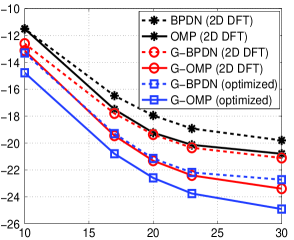
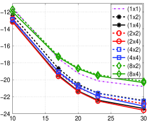
Figure 4: MSE versus SNR for various compressive estimators in the SISO case: (a) using different CS reconstruction methods, the 2D DFT basis and the optimized basis, and block size $\Delta m^{\prime}\!\times\Delta i^{\prime}=1\!\times 4$; (b) using G-OMP, the 2D DFT basis, and different block sizes $\Delta m^{\prime}\!\times\Delta i^{\prime}$.

Fig. 4 shows the channel estimation MSE versus the SNR. The blocks $\mathcal{B}_{b}$ of the delay-Doppler tiling used in the definition of group sparsity (see Section IV-B) were of size $\Delta m^{\prime}\!\times\Delta i^{\prime}=1\!\times 4$. For the proposed channel estimator, we used both the 2D DFT basis and the optimized basis. It is seen that exploiting the inherent group sparsity of the channel yields a substantial reduction of the MSE, and an additional substantial MSE reduction is obtained by using the optimized basis.

Fig. 4 shows the MSE versus the SNR for the proposed channel estimator using G-OMP, the 2D DFT basis, and different block sizes $\Delta m^{\prime}\!\times\Delta i^{\prime}$ (note that the case $\Delta m^{\prime}\!\times\Delta i^{\prime}=1\!\times 1$ corresponds to the conventional compressive channel estimator of [17]). One can observe a strong dependence of the performance on the block size. This can be explained by the fact that if the blocks $\mathcal{B}_{b}$ are chosen too large in a certain direction, many entries not belonging to the (effective) support of $\tilde{\mathbf{x}}$ in (40) will be assigned nonzero values during reconstruction since they belong to blocks containing some large entries.

VII-C Performance Gains Due to Exploiting Joint Sparsity

Next, we consider the MIMO case. We first compare our channel estimator leveraging only joint sparsity (hereafter referred to as MCS channel estimator, cf. also [32]) with the conventional compressive channel estimator. At this point, the proposed estimator does not exploit group sparsity; it uses G-BPDN or DCS-SOMP, where G-BPDN is based on blocks $\mathcal{B}_{b}$ of size $\Delta m^{\prime}\!\times\Delta i^{\prime}=1\!\times 1$ but runs in MGCS mode in order to exploit joint sparsity (this will be abbreviated as “MG-BPDN-$1\!\times\!1$”). The reason for choosing MG-BPDN-$1\!\times\!1$ instead of M-BPDN is its ability to handle the different measurement matrices $\mathbf{\Phi}^{(\theta)}$ in (14) (note that our application involves different measurement matrices, cf. (40)). As a performance benchmark, we also consider a conventional compressive channel estimator that uses BPDN or OMP for each component channel individually.

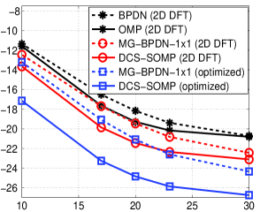
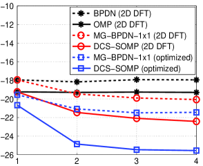
Figure 5: MSE performance (a) versus SNR for a $2\!\times\!2$ MIMO system, (b) versus the number $N_{\text{T}}=N_{\text{R}}$ of transmit/receive antennas at an SNR of 20 dB.

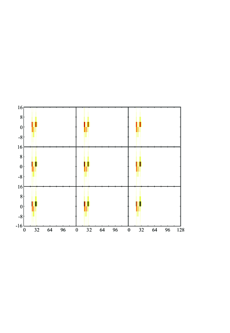
Figure 6: Visualization of the joint group sparsity of the 2D DFT coefficients $F_{m,i}^{(\theta)}$ for a $3\!\times\!3$ MIMO system and block size $\Delta m^{\prime}\!\times\Delta i^{\prime}=1\!\times 4$.

Fig. 5 shows the MSE versus the SNR for a MIMO system with $N_{\text{T}}\!=\!N_{\text{R}}\!=\!2$ transmit/receive antennas. It is seen that substantial reductions of the MSE are obtained by exploiting the channel’s joint sparsity via MCS methods and, additionally, by using the optimized basis. Fig. 5 shows the MSE versus $N_{\text{T}}\!=\!N_{\text{R}}\in\{1,2,3,4\}$ at an SNR of 20 dB. The MSE is seen to decrease for an increasing number of antennas. This is because the estimation of the joint support becomes more accurate when a larger number of jointly sparse signals are available; this behavior has been studied in [59] for M-BPDN and SOMP. The flattening of the MSE curves is caused by the fact that the component channels, besides being jointly sparse in the sense of similar effective supports, are also similar with respect to the values of their nonzero entries. As explained in [59], the case where all jointly sparse signals are equal is a worst-case scenario for MCS, since no additional support information can be gained from additional signals. In our case, this effect is alleviated since the jointly sparse signals are observed through different measurement matrices $\mathbf{\Phi}^{(s)}\!$, $s\in\{1,\dots,N_{\text{T}}\}$. The MSE of the conventional compressive channel estimator is essentially independent of the number of antennas.

VII-D Performance Gains Due to Exploiting Joint Group Sparsity

Next, we consider the case where the proposed channel estimator fully exploits the available structure, i.e., the joint group sparsity of the $F_{m,i}^{(\theta)}$ or $G_{m,i}^{(\theta)}$. Fig. 6 shows the energy of the 2D DFT coefficients $F_{m,i}^{(\theta)}$ accumulated in blocks $\mathcal{B}_{b}$ of size $\Delta m^{\prime}\!\times\Delta i^{\prime}=1\!\times 4$ for the nine component channels $\theta=$$(1,1),(1,2),\ldots,(3,3)$ of a $3\!\times\!3$ MIMO system. It is seen that the $F_{m,i}^{(\theta)}$ are effectively supported on the same blocks for all $\theta$. This demonstrates the strong available joint group sparsity, and thus suggests that significant performance gains can be obtained by using MGCS channel estimation.

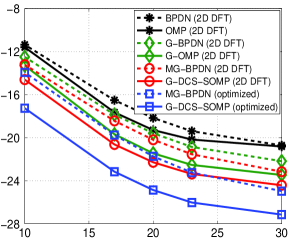
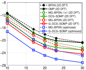
Figure 7: MSE versus SNR for a $2\!\times\!2$ MIMO system: (a) MGCS estimators, GCS estimators, and conventional compressive estimators; (b) MGCS estimators, MCS estimators, and conventional compressive estimators.

To assess the actual gains, we simulated MGCS estimators, GCS estimators (exploiting only group sparsity), MCS estimators (exploiting only joint sparsity), and conventional compressive estimators for a $2\!\times\!2$ MIMO system. We used the 2D DFT basis and, for the MGCS estimator, additionally an optimized basis. Fig. 7 shows the MSE versus the SNR. Both parts (a) and (b) show identical MSE curves for the MGCS estimators (using MG-BPDN or G-DCS-SOMP) and the conventional compressive estimators (using BPDN or OMP); however, part (a) compares these curves with the GCS estimators (using G-BPDN or G-OMP) and part (b) with the MCS estimators (using MG-BPDN-$1\!\times\!1$ or DCS-SOMP). For the MGCS and GCS estimators, the blocks $\mathcal{B}_{b}$ were of size $\Delta m^{\prime}\!\times\Delta i^{\prime}\!=1\!\times 4$. It can be seenthat exploiting group or joint sparsity separately already outperforms conventional compressive channel estimation. Moreover, substantial additional gains are obtained by exploiting the joint group sparsity structure through the proposed MGCS estimator, and even larger gains are achieved when the MGCS estimator is used with an optimized basis.

VIII Conclusion

For multicarrier MIMO systems transmitting over doubly selective channels, we demonstrated that leakage effects induce an approximate group sparsity structure of the individual component channels in the delay-Doppler domain. We also showed that the effective delay-Doppler supports of the component channels overlap significantly, which implies that these channels are approximately jointly group sparse. Using the methodology of multichannel group sparse compressed sensing (MGCS), we then devised a compressive channel estimator that leverages the joint group sparsity structure. We also presented an upper bound on the MSE of this estimator, and we analyzed the estimator’s computational complexity. Furthermore, we proposed an optimization of a basis involved in the estimator that aims at maximizing joint group sparsity. We presented an iterative approximate optimization algorithm consisting of a sequence of convex programming problems. Statistical information about the channel can be incorporated in this algorithm if available.

Simulations using a geometry-based channel simulator demonstrated substantial performance gains over conventional compressive channel estimation. Large gains can already be obtained by exploiting only group sparsity or joint sparsity, and the combined MGCS approach yields an even larger gain. An additional gain results from the proposed basis optimization.

Appendix A:  Proof of Inequality (31)

Supposing, without loss of generality, that $\left\lVert\mathbf{a}\right\rVert_{2}\geq\left\lVert\mathbf{b}\right\rVert_{2}$, the inequality (31) is equivalent to

$$\left\lVert\frac{\mathbf{a}}{\left\lVert\mathbf{a}\right\rVert_{2}}-\frac{\mathbf{b}}{\left\lVert\mathbf{b}\right\rVert_{2}}\right\rVert_{2}^{2}\hskip 0.85358pt\leq\,\frac{\left\lVert\mathbf{a}-\mathbf{b}\right\rVert_{2}^{2}}{\left\lVert\mathbf{b}\right\rVert_{2}^{2}}\;,\vspace{-.5mm}$$

and, expanding the squared norms, to

$$2-2\hskip 0.85358pt\frac{\mathbf{a}^{T}\mathbf{b}}{\left\lVert\mathbf{a}\right\rVert_{2}\left\lVert\mathbf{b}\right\rVert_{2}}\,\leq\,\frac{\left\lVert\mathbf{a}\right\rVert_{2}^{2}+\left\lVert\mathbf{b}\right\rVert_{2}^{2}-2\hskip 0.85358pt\mathbf{a}^{T}\mathbf{b}}{\left\lVert\mathbf{b}\right\rVert_{2}^{2}}\;.$$

Rearranging terms, this is furthermore equivalent to

$$\frac{\left\lVert\mathbf{a}\right\rVert_{2}^{2}}{\left\lVert\mathbf{b}\right\rVert_{2}^{2}}\hskip 0.85358pt\hskip 0.85358pt+\hskip 0.85358pt2\hskip 0.85358pt\frac{\mathbf{a}^{T}\mathbf{b}}{\left\lVert\mathbf{b}\right\rVert_{2}}\left(\frac{1}{\left\lVert\mathbf{a}\right\rVert_{2}}-\frac{1}{\left\lVert\mathbf{b}\right\rVert_{2}}\right)\hskip 0.85358pt\geq\hskip 0.85358pt1\,.$$ (58)

To prove (58), we use the Cauchy-Schwarz inequality, noting that $\frac{1}{\left\lVert\mathbf{a}\right\rVert_{2}}-\frac{1}{\left\lVert\mathbf{b}\right\rVert_{2}}\leq 0$:

$$\frac{\left\lVert\mathbf{a}\right\rVert_{2}^{2}}{\left\lVert\mathbf{b}\right\rVert_{2}^{2}}\hskip 0.85358pt\hskip 0.85358pt+\hskip 0.85358pt2\hskip 0.85358pt\frac{\mathbf{a}^{T}\mathbf{b}}{\left\lVert\mathbf{b}\right\rVert_{2}}\left(\frac{1}{\left\lVert\mathbf{a}\right\rVert_{2}}-\frac{1}{\left\lVert\mathbf{b}\right\rVert_{2}}\right)$$

$$\hskip 19.91692pt\geq\,\frac{\left\lVert\mathbf{a}\right\rVert_{2}^{2}}{\left\lVert\mathbf{b}\right\rVert_{2}^{2}}\hskip 0.85358pt\hskip 0.85358pt+\hskip 0.85358pt2\hskip 0.85358pt\frac{\left\lVert\mathbf{a}\right\rVert_{2}\left\lVert\mathbf{b}\right\rVert_{2}}{\left\lVert\mathbf{b}\right\rVert_{2}}\left(\frac{1}{\left\lVert\mathbf{a}\right\rVert_{2}}-\frac{1}{\left\lVert\mathbf{b}\right\rVert_{2}}\right)$$

$$\hskip 19.91692pt=\,\frac{\left\lVert\mathbf{a}\right\rVert_{2}^{2}}{\left\lVert\mathbf{b}\right\rVert_{2}^{2}}\hskip 0.85358pt\hskip 0.85358pt+\hskip 0.85358pt2\left(1-\frac{\left\lVert\mathbf{a}\right\rVert_{2}}{\left\lVert\mathbf{b}\right\rVert_{2}}\right)$$

$$\hskip 19.91692pt=\,\frac{\left\lVert\mathbf{a}\right\rVert_{2}^{2}}{\left\lVert\mathbf{b}\right\rVert_{2}^{2}}\hskip 0.85358pt-\hskip 0.85358pt2\frac{\left\lVert\mathbf{a}\right\rVert_{2}}{\left\lVert\mathbf{b}\right\rVert_{2}}\hskip 0.85358pt+\hskip 0.85358pt2$$

$$\hskip 19.91692pt=\hskip 0.85358pt\left(\frac{\left\lVert\mathbf{a}\right\rVert_{2}}{\left\lVert\mathbf{b}\right\rVert_{2}}-1\right)^{\!2}+1$$

$$\hskip 19.91692pt\geq\,1\hskip 0.85358pt.$$

Appendix B:  Proof of Theorem 1

Let $\mathbf{h}^{(\theta)}\!\triangleq\operatorname{{rvec}}_{l,k}\big{\{}H^{(\theta)}_{l,k}\big{\}}\in\mathbb{C}^{KL}\!$, i.e., ${[\mathbf{h}^{(\theta)}]}_{k+lK+1}\!=H^{(\theta)}_{l,k}$;let $\mathbf{f}^{(\theta)}\triangleq\operatorname{{rvec}}_{m,i}\big{\{}F_{m,i}^{(\theta)}\big{\}}\in\mathbb{C}^{KL}$, i.e., ${[\mathbf{f}^{(\theta)}]}_{mL+i+L/2+1}=F_{m,i}^{(\theta)}$; and let $\mathbf{U}_{\textnormal{F}}\in\mathbb{C}^{KL\times KL}$ be the unitary matrix with entries ${[\mathbf{U}_{\textnormal{F}}]}_{k+lK+1,\hskip 0.85358ptmL+i+L/2+1}=\frac{1}{\sqrt{KL}}\,e^{-j2\pi(\frac{km}{K}-\frac{li}{L})}$, where $l\in\{0,\dots,L-1\}$, $k\in\{0,\dots,K-1\}$, $m\in\{0,\dots,K-1\}$, and $i\in\{-L/2,\dots,L/2-1\}$. Then, (8) can be written as $\mathbf{h}^{(\theta)}=\sqrt{KL}\,\mathbf{U}_{\textnormal{F}}\hskip 0.85358pt\mathbf{f}^{(\theta)}$, which implies

$${\|\mathbf{h}^{(\theta)}\|}_{2}\hskip 0.85358pt=\hskip 0.85358pt\sqrt{KL}\,{\|\mathbf{f}^{(\theta)}\|}_{2}\,.\vspace{-1mm}$$ (59)

Furthermore, let $\mathbf{h}^{(\theta)}_{\Delta}\!\triangleq\operatorname{{rvec}}_{\lambda,\kappa}\big{\{}H^{(\theta)}_{\lambda\Delta L,\kappa\Delta K}\big{\}}\!\in\!\mathbb{C}^{JD}$, i.e., ${[\mathbf{h}^{(\theta)}_{\Delta}]}_{\kappa+\lambda D+1}=H^{(\theta)}_{\lambda\Delta L,\kappa\Delta K}$; let $\tilde{\mathbf{f}}^{(\theta)}\in\mathbb{C}^{JD}$ be defined by ${[\tilde{\mathbf{f}}^{(\theta)}]}_{mJ+i+J/2+1}=F_{m,i}^{(\theta)}$ (this is the subvector of $\mathbf{f}^{(\theta)}$ that corresponds to the restriction of $F_{m,i}^{(\theta)}$ to $\{0,\dots,D-1\}\times\{-J/2,\dots,J/2-1\}$); and let $\tilde{\mathbf{U}}_{\textnormal{F}}\in\mathbb{C}^{JD\times JD}$ be the unitary matrix with entries ${[\tilde{\mathbf{U}}_{\textnormal{F}}]}_{\kappa+\lambda D+1,\hskip 0.85358ptmJ+i+J/2+1}=\frac{1}{\sqrt{JD}}\,e^{-j2\pi(\frac{\kappa m}{D}-\frac{\lambda i}{J})}$, where $\kappa\in\{0,\dots,D-\!1\}$, $\lambda\in\{0,\dots,$$J-\!1\}$, $m\in\{0,\dots,D-\!1\}$, and $i\in\{-J/2,\dots,J/2-\!1\}$. Then, we can rewrite (34) as $\mathbf{h}^{(\theta)}_{\Delta}=\sqrt{JD}\,\tilde{\mathbf{U}}_{\textnormal{F}}\hskip 0.85358pt\tilde{\mathbf{f}}^{(\theta)}$. We thus obtain

$${\|\mathbf{h}^{(\theta)}_{\Delta}\|}_{2}\hskip 0.85358pt=\hskip 0.85358pt\sqrt{JD}\,{\|\tilde{\mathbf{f}}^{(\theta)}\|}_{2}\hskip 0.85358pt=\hskip 0.85358pt\sqrt{JD}\,{\|\mathbf{f}^{(\theta)}\|}_{2}\,,$$ (60)

since $\mathbf{f}^{(\theta)}$ differs from its subvector $\tilde{\mathbf{f}}^{(\theta)}$ only by additional zero entries. Finally, let $\mathbf{g}^{(\theta)}\triangleq\operatorname{{rvec}}_{m,i}\big{\{}G_{m,i}^{(\theta)}\big{\}}\in\mathbb{C}^{JD}$, i.e., ${[\mathbf{g}^{(\theta)}]}_{mJ+i+J/2+1}=G_{m,i}^{(\theta)}$, and let $\mathbf{U}\in\mathbb{C}^{JD\times JD}$ be the unitary matrix with entries ${[\mathbf{U}]}_{\kappa+\lambda D+1,\hskip 0.85358ptmJ+i+J/2+1}=u_{m,i}[\lambda,\kappa]$. Then (35) can be written as $\mathbf{h}^{(\theta)}_{\Delta}=\mathbf{U}\mathbf{g}^{(\theta)}$, which implies

$${\|\mathbf{h}^{(\theta)}_{\Delta}\|}_{2}\hskip 0.85358pt=\hskip 0.85358pt{\|\mathbf{g}^{(\theta)}\|}_{2}\,.\vspace{.5mm}$$ (61)

Combining (59)–(61), we obtain ${\|\mathbf{h}^{(\theta)}\|}_{2}=\sqrt{\frac{KL}{JD}}\,{\|\mathbf{g}^{(\theta)}\|}_{2}$ and, furthermore,

$$\Bigg{(}\sum_{l=0}^{L-1}\sum_{k=0}^{K-1}\big{|}\hat{H}^{(\theta)}_{l,k}-H^{(\theta)}_{l,k}\big{|}^{2}\Bigg{)}^{\!\!1/2}\! =\hskip 0.85358pt\big{\|}\hat{\mathbf{h}}^{(\theta)}-\mathbf{h}^{(\theta)}\big{\|}_{2}$$

$$=\hskip 0.85358pt\sqrt{\frac{KL}{JD}}\,\big{\|}\hat{\mathbf{g}}^{(\theta)}-\mathbf{g}^{(\theta)}\big{\|}_{2}\,,$$ (62)

where $\hat{\mathbf{h}}^{(\theta)}\triangleq\operatorname{{rvec}}_{l,k}\big{\{}\hat{H}^{(\theta)}_{l,k}\big{\}}$ and $\hat{\mathbf{g}}^{(\theta)}\triangleq\operatorname{{rvec}}_{m,i}\big{\{}\hat{G}^{(\theta)}_{m,i}\big{\}}$ denote the estimates of $\mathbf{h}^{(\theta)}$ and $\mathbf{g}^{(\theta)}$, respectively.

Next, let $\tilde{\mathbf{G}}_{m,i}$ be the $N_{\text{R}}\!\times\!N_{\text{T}}$ matrix with entries $\big{[}\tilde{\mathbf{G}}_{m,i}\big{]}_{r,s}\!\triangleq\tilde{G}_{m,i}^{(r,s)}$ for $r\in\{1,\dots,N_{\text{R}}\}$ and $s\in\{1,\dots,N_{\text{T}}\}$, and let (cf. (39))

$$\tilde{\mathbf{g}}^{(\theta)}\hskip 0.85358pt\triangleq\,\operatorname{{rvec}}_{m,i}\big{\{}\tilde{G}_{m,i}^{(\theta)}\big{\}}\hskip 0.85358pt=\hskip 0.85358pt\sqrt{\frac{JD}{Q}}\,\mathbf{x}^{(\theta)}.\vspace{-1mm}$$ (63)

By the definition of $\tilde{G}_{m,i}^{(\theta)}$ in (36), we have $\tilde{\mathbf{G}}_{m,i}=\mathbf{G}_{m,i}\hskip 0.85358pt\mathbf{P}$ and, in turn, $\mathbf{G}_{m,i}=\tilde{\mathbf{G}}_{m,i}\hskip 0.85358pt\mathbf{P}^{-1}$. Similarly, we have $\hat{\mathbf{G}}_{m,i}=\hat{\tilde{\mathbf{G}}}_{m,i}\hskip 0.85358pt\mathbf{P}^{-1}$, where $\hat{\tilde{\mathbf{G}}}_{m,i}$ denotes the estimate of $\tilde{\mathbf{G}}_{m,i}$ (cf. step 2 in Section V-B). We then obtain

$$\sum_{\theta\in\Theta}\big{\|}\hat{\mathbf{g}}^{(\theta)}-\mathbf{g}^{(\theta)}\big{\|}_{2}^{2}\, \overset{(a)}{\,=\,}\,\sum_{m=0}^{D-1}\sum_{i=-J/2}^{J/2-1}\big{\|}\hat{\mathbf{G}}_{m,i}-\mathbf{G}_{m,i}\big{\|}_{\text{F}}^{2}$$

$$\,=\,\,\sum_{m=0}^{D-1}\sum_{i=-J/2}^{J/2-1}\big{\|}\big{(}\hat{\tilde{\mathbf{G}}}_{m,i}-\tilde{\mathbf{G}}_{m,i}\big{)}\mathbf{P}^{-1}\big{\|}_{\text{F}}^{2}$$

$$\,\overset{(b)}{\leq}\,\sum_{m=0}^{D-1}\sum_{i=-J/2}^{J/2-1}\big{\|}\hat{\tilde{\mathbf{G}}}_{m,i}-\tilde{\mathbf{G}}_{m,i}\big{\|}_{\text{F}}^{2}\,\|\mathbf{P}^{-1}\|^{2}$$

$$\overset{(c)}{\,=\,}\|\mathbf{P}^{-1}\|^{2}\sum_{\theta\in\Theta}\big{\|}\hat{\tilde{\mathbf{g}}}^{(\theta)}-\tilde{\mathbf{g}}^{(\theta)}\big{\|}_{2}^{2}$$

$$\,=\,\|\mathbf{P}^{-1}\|^{2}\,\frac{JD}{Q}\sum_{\theta\in\Theta}\big{\|}\hat{\mathbf{x}}^{(\theta)}-\mathbf{x}^{(\theta)}\big{\|}_{2}^{2}$$

$$\,=\,\frac{JD}{Q}\,\|\mathbf{P}^{-1}\|^{2}\,{\|\mathbf{\hat{x}}-\mathbf{x}\|}_{2}^{2}\;,$$ (64)

where $\left\lVert\cdot\right\rVert$ denotes the spectral norm [67], $\mathbf{x}\triangleq\big{(}\mathbf{x}^{(\theta_{1})\hskip 0.85358ptT}\cdots$$\mathbf{x}^{(\theta_{N_{\text{T}}N_{\text{R}}})\hskip 0.85358ptT}\big{)}^{T}$, and $\mathbf{\hat{x}}\triangleq\big{(}\hat{\mathbf{x}}^{(\theta_{1})\hskip 0.85358ptT}\cdots\,\hat{\mathbf{x}}^{(\theta_{N_{\text{T}}N_{\text{R}}})\hskip 0.85358ptT}\big{)}^{T}$. Here, $(a)$ and $(c)$ are obtained by reordering the sums, and $(b)$ follows by the general inequality ${\|\mathbf{A}\mathbf{B}\|}_{\text{F}}\leq{\|\mathbf{A}\|}_{\text{F}}\hskip 0.85358pt\|\mathbf{B}\|$ [67, problem 20 in ch. 5.6]. A combination of (62) and (64) then yields

$$E \,=\hskip 0.85358pt\Bigg{(}\sum_{\theta\in\Theta}\sum_{l=0}^{L-1}\sum_{k=0}^{K-1}\big{|}\hat{H}^{(\theta)}_{l,k}-H^{(\theta)}_{l,k}\big{|}^{2}\Bigg{)}^{\!\!1/2}$$

$$\,=\,\bigg{(}\sum_{\theta\in\Theta}\frac{KL}{JD}\,\big{\|}\hat{\mathbf{g}}^{(\theta)}-\mathbf{g}^{(\theta)}\big{\|}_{2}^{2}\bigg{)}^{\!1/2}$$

$$\,\leq\,\sqrt{\frac{KL}{Q}}\,\|\mathbf{P}^{-1}\|\,{\|\mathbf{\hat{x}}-\mathbf{x}\|}_{2}\,.$$ (65)

We now consider the first part of Theorem 1, concerning the use of G-BPDN for MGCS reconstruction. We will use the following result on the performance of G-BPDN. Let $\mathbf{\hat{x}}$ denote the solution of (11), and let $\mathbf{x}^{S|\mathcal{J}}$ denote the best group $S$-sparse approximation of $\mathbf{x}$ with respect to $\mathcal{J}$, i.e., the $\mathbf{x}^{\prime}\!\in\Sigma_{S|\mathcal{J}}$ minimizing ${\|\mathbf{x}^{\prime}\!-\mathbf{x}\|}_{2|\mathcal{J}}$. Then, as shown in [36], if $\mathbf{y}$ satisfies ${\|\mathbf{\Phi}\mathbf{x}-\mathbf{y}\|}_{2}={\|\mathbf{z}\|}_{2}\leq\epsilon$ and $\mathbf{\Phi}$ satisfies the group restricted isometry property of order $2S$ with G-RIC $\delta_{2S|\mathcal{J}}\leq\sqrt{2}-1$, then

$${\|\mathbf{\hat{x}}-\mathbf{x}\|}_{2}\,\leq\,\frac{c_{0}}{\sqrt{S}}\,{\|\mathbf{x}-\mathbf{x}^{S|\mathcal{J}}\|}_{2|\mathcal{J}}\hskip 0.85358pt+\hskip 0.85358ptc_{1}\epsilon\,,\vspace{-1mm}$$ (66)

with $c_{0}$ and $c_{1}$ as given in Theorem 1. This result bounds the reconstruction error ${\|\mathbf{\hat{x}}-\mathbf{x}\|}_{2}$ in terms of ${\|\mathbf{x}-\mathbf{x}^{S|\mathcal{J}}\|}_{2|\mathcal{J}}$, which characterizes the deviation of $\mathbf{x}$ from being group $S$-sparse with respect to $\mathcal{J}$, and in terms of $\epsilon$.

Recall (18), i.e., the fact that the G-RIC of the stacked measurement matrix $\mathbf{\Phi}$ in (16) with respect to the associated partition $\tilde{\mathcal{J}}$ (cf. (15)) satisfies $\delta_{S|\tilde{\mathcal{J}}}=\max_{s}\delta_{S|\mathcal{J}}^{(s)}$. Our assumption on the $\mathbf{\Phi}^{(s)}$, i.e., $\delta_{2S|\mathcal{J}}^{(s)}\leq\sqrt{2}-1$ for all $s\in\{1,\dots,N_{\text{T}}\}$, then implies that $\delta_{2S|\tilde{\mathcal{J}}}\leq\sqrt{2}-1$. Thus, with our additional assumption that $\big{(}\sum_{\theta\in\Theta}{\|\mathbf{z}^{(\theta)}\|}_{2}^{2}\big{)}^{1/2}\leq\epsilon$, we have (cf. (66)) ${\|\mathbf{\hat{x}}-\mathbf{x}\|}_{2}\leq\frac{c_{0}}{\sqrt{S}}\hskip 0.85358pt{\|\mathbf{x}-\mathbf{x}^{S|\tilde{\mathcal{J}}}\|}_{2|\tilde{\mathcal{J}}}+c_{1}\epsilon$. Inserting into (65) yields the bound

$$E\,\leq\,\sqrt{\frac{KL}{Q}}\,\|\mathbf{P}^{-1}\|\,\bigg{(}\frac{c_{0}}{\sqrt{S}}\hskip 0.85358pt{\|\mathbf{x}-\mathbf{x}^{S|\tilde{\mathcal{J}}}\|}_{2|\tilde{\mathcal{J}}}+c_{1}\epsilon\bigg{)}\,.$$ (67)

Now recall that $\mathbf{x}^{S|\tilde{\mathcal{J}}}$ is the group $S$-sparse vector $\mathbf{x}^{\prime}\!\in\Sigma_{S|\tilde{\mathcal{J}}}$ minimizing $\|\mathbf{x}-\mathbf{x}^{\prime}\|_{2|\tilde{\mathcal{J}}}$, and note that the subvectors $\mathbf{x}^{S|\tilde{\mathcal{J}}}[b]$ coincide with the subvectors $\mathbf{x}[b]$ for $b\in\mathcal{T}$, where $\mathcal{T}\subseteq\{1,\dots,B\}$ denotes the set of those $S$ group indices that yield the largest norms ${\|\mathbf{x}[b]\|}_{2}\hskip 0.85358pt$, and $\mathbf{x}^{S|\tilde{\mathcal{J}}}[b]=\mathbf{0}$ for $b\notin\mathcal{T}$. Therefore,

$${\big{\|}\mathbf{x}-\mathbf{x}^{S|\tilde{\mathcal{J}}}\big{\|}}_{2|\tilde{\mathcal{J}}}=\sum_{b\hskip 0.85358pt=1}^{B}\big{\|}\mathbf{x}[b]-\mathbf{x}^{S|\tilde{\mathcal{J}}}[b]\big{\|}_{2}=\sum_{b\hskip 0.85358pt\notin\mathcal{T}}\|\mathbf{x}[b]\|_{2}\,.$$

Moreover, by the definition of $\mathcal{T}$, we have ${\|\mathbf{x}[b]\|}_{2}\geq{\|\mathbf{x}[b^{\prime}]\|}_{2}$ for all $b\!\in\!\mathcal{T}$ and $b^{\prime}\!\notin\!\mathcal{T}$, which yields $\sum_{b\hskip 0.85358pt\in\mathcal{T}}{\|\mathbf{x}[b]\|}_{2}\geq\sum_{b\hskip 0.85358pt\in\mathcal{T}^{\prime}}{\|\mathbf{x}[b]\|}_{2}$ for any set $\mathcal{T}^{\prime}\!\subseteq\{1,\dots,B\}$ of cardinality $|\mathcal{T}^{\prime}|=|\mathcal{T}|=S$, and in turn $\sum_{b\hskip 0.85358pt\notin\mathcal{T}}{\|\mathbf{x}[b]\|}_{2}\hskip 0.85358pt\leq\sum_{b\hskip 0.85358pt\notin\mathcal{T}^{\prime}}{\|\mathbf{x}[b]\|}_{2}$. Inserting into (LABEL:bestappr) gives

$${\big{\|}\mathbf{x}-\mathbf{x}^{S|\tilde{\mathcal{J}}}\big{\|}}_{2|\tilde{\mathcal{J}}}\hskip 0.85358pt\leq\sum_{b\hskip 0.85358pt\notin\mathcal{T}^{\prime}}\!{\|\mathbf{x}[b]\|}_{2}\,,\vspace{-1mm}$$ (69)

for any such set $\mathcal{T}^{\prime}$ of cardinality $S$. Then, with $\mathcal{S}$ defined as in Section V-C, we obtain

$${\big{\|}\mathbf{x}-\mathbf{x}^{S|\tilde{\mathcal{J}}}\big{\|}}_{2|\tilde{\mathcal{J}}} \overset{(a)}{\,\leq\,}\sum_{b\hskip 0.85358pt\notin\mathcal{S}}{\|\mathbf{x}[b]\|}_{2}$$

$$\!\overset{\eqref{x_b_theta_vector}}{\,\,=\,\,}\sum_{b\hskip 0.85358pt\notin\mathcal{S}}\bigg{(}\sum_{\theta\in\Theta}\big{\|}\mathbf{x}^{(\theta)}[b]\big{\|}_{2}^{2}\bigg{)}^{\!1/2}$$

$$\!\overset{\eqref{eq_tildeg_G_x}}{\,\,=\,\,}\sqrt{\frac{Q}{JD}}\sum_{b\hskip 0.85358pt\notin\mathcal{S}}\bigg{(}\sum_{\theta\in\Theta}\big{\|}\tilde{\mathbf{g}}^{(\theta)}[b]\big{\|}_{2}^{2}\bigg{)}^{\!1/2}\;,$$ (70)

where $(a)$ follows from (69) and the fact that $|\mathcal{S}|=S$. Now for each group $\mathcal{I}_{b}$ of $\mathcal{J}$ we have (with $\mathcal{B}_{b}=\mathsf{S}^{-1}(\mathcal{I}_{b})$, cf. (33) and the discussion following (33))

$$\sum_{\theta\in\Theta}\big{\|}\tilde{\mathbf{g}}^{(\theta)}[b]\big{\|}_{2}^{2} \hskip 0.85358pt\overset{(a)}{\,=\,}\hskip 0.85358pt\sum_{\theta\in\Theta}\sum_{(m,i)\in\mathcal{B}_{b}}\!\!|\tilde{G}_{m,i}^{(\theta)}|^{2}$$

$$\hskip 0.85358pt\overset{(b)}{\,=\,}\hskip 0.85358pt\!\!\!\sum_{(m,i)\in\mathcal{B}_{b}}\!\!\big{\|}\tilde{\mathbf{G}}_{m,i}\big{\|}_{\textnormal{F}}^{2}$$

$$\hskip 0.85358pt\overset{(c)}{\leq}\!\sum_{(m,i)\in\mathcal{B}_{b}}\!\!{\|\mathbf{G}_{m,i}\|}_{\textnormal{F}}^{2}\hskip 0.85358pt\|\mathbf{P}\|^{2}$$

$$\overset{(d)}{\,=\,}\hskip 0.85358pt\|\mathbf{P}\|^{2}\sum_{\theta\in\Theta}\big{\|}\mathbf{g}^{(\theta)}[b]\big{\|}_{2}^{2}\,.$$ (71)

Here, $(a)$ follows from $\tilde{\mathbf{g}}^{(\theta)}=\operatorname{{rvec}}_{m,i}\big{\{}\tilde{G}_{m,i}^{(\theta)}\big{\}}$, $(b)$ follows from $\tilde{G}_{m,i}^{(r,s)}=\big{[}\tilde{\mathbf{G}}_{m,i}\big{]}_{r,s}$, $(c)$ follows from $\tilde{\mathbf{G}}_{m,i}=\mathbf{G}_{m,i}\hskip 0.85358pt\mathbf{P}$ and ${\|\mathbf{AB}\|}_{\textnormal{F}}\leq{\|\mathbf{A}\|}_{\textnormal{F}}\|\mathbf{B}\|$, and $(d)$ follows from $\mathbf{g}^{(\theta)}=\operatorname{{rvec}}_{m,i}\big{\{}G_{m,i}^{(\theta)}\big{\}}$. Inserting (71) into (70) yields

$${\big{\|}\mathbf{x}-\mathbf{x}^{S|\tilde{\mathcal{J}}}\big{\|}}_{2|\tilde{\mathcal{J}}} \,\leq\,\sqrt{\frac{Q}{JD}}\,\|\mathbf{P}\|\sum_{b\hskip 0.85358pt\notin\mathcal{S}}\bigg{(}\hskip 0.85358pt\sum_{\theta\in\Theta}\big{\|}\mathbf{g}^{(\theta)}[b]\big{\|}_{2}^{2}\bigg{)}^{\!1/2}$$

$$\overset{(a)}{\,=\,}\hskip 0.85358pt\sqrt{\frac{Q}{JD}}\,\|\mathbf{P}\|\,C_{G,\mathcal{S},\mathcal{J}}\,,$$ (72)

where $(a)$ follows from $\mathbf{g}^{(\theta)}=\operatorname{{rvec}}_{m,i}\big{\{}G_{m,i}^{(\theta)}\big{\}}$ and (42). Inserting this bound into (67) finally yields

$$E\,\leq\,c_{0}\hskip 0.85358pt\sqrt{\frac{KL}{JD}}\hskip 0.85358pt\|\mathbf{P}^{-1}\|\left\lVert\mathbf{P}\right\rVert\frac{C_{G,\mathcal{S},\mathcal{J}}}{\sqrt{S}}+\hskip 0.85358ptc_{1}\hskip 0.85358pt\sqrt{\frac{KL}{Q}}\hskip 0.85358pt\|\mathbf{P}^{-1}\|\hskip 0.85358pt\epsilon\,,\vspace{-2mm}$$

which is (44).

Next, we consider the second part of Theorem 1, concerning the use of G-CoSaMP for MGCS reconstruction. We will use the following result on the performance of G-CoSaMP, obtained by specializing results from [39]. Consider a partition $\mathcal{J}$ with groups of equal size. If $\mathbf{y}$ satisfies ${\|\mathbf{\Phi}\mathbf{x}-\mathbf{y}\|}_{2}\leq\epsilon$ and $\mathbf{\Phi}$ satisfies the group restricted isometry property of order $4S$ with respect to $\mathcal{J}$ with G-RIC $\delta_{4S|\mathcal{J}}\leq 0.1$, the result $\hat{\mathbf{x}}$ of G-CoSaMP after $j$ iteration steps satisfies

$${\|\hat{\mathbf{x}}-\mathbf{x}\|}_{2}\,\leq\,\frac{1}{2^{j}}\hskip 0.85358pt{\|\mathbf{x}\|}_{2}\hskip 0.85358pt+\hskip 0.85358pt20\hskip 0.85358pt\bigg{(}1+\frac{1}{\sqrt{S}}\bigg{)}{\|\mathbf{x}-\mathbf{x}^{S|\mathcal{J}}\|}_{2|\mathcal{J}}\hskip 0.85358pt+\hskip 0.85358pt20\hskip 0.85358pt\epsilon\,.$$ (73)

Under our assumption on the $\mathbf{\Phi}^{(s)}$, i.e., $\delta_{4S|\mathcal{J}}^{(s)}\leq 0.1$, the G-RIC of the stacked measurement matrix $\mathbf{\Phi}$ with respect to the associated partition $\tilde{\mathcal{J}}$ satisfies $\delta_{4S|\tilde{\mathcal{J}}}\leq 0.1$ (cf. (18)). With our additional assumption that $\big{(}\sum_{\theta\in\Theta}{\|\mathbf{z}^{(\theta)}\|}_{2}^{2}\big{)}^{1/2}\leq\epsilon$, we obtain (cf. (73)) ${\|\mathbf{\hat{x}}-\mathbf{x}\|}_{2}\leq\frac{1}{2^{j}}\hskip 0.85358pt{\|\mathbf{x}\|}_{2}+20\hskip 0.85358pt\big{(}1+\frac{1}{\sqrt{S}}\big{)}{\|\mathbf{x}-\mathbf{x}^{S|\tilde{\mathcal{J}}}\|}_{2|\tilde{\mathcal{J}}}+20\hskip 0.85358pt\epsilon$. Inserting into (65) yields the bound

$$E\,\leq\,\sqrt{\frac{KL}{Q}}\,\|\mathbf{P}^{-1}\|\,\bigg{[}\frac{1}{2^{j}}\hskip 0.85358pt{\|\mathbf{x}\|}_{2}\hskip 0.85358pt+\hskip 0.85358pt20\hskip 0.85358pt\bigg{(}1+\frac{1}{\sqrt{S}}\bigg{)}$$

$$\hskip 105.27519pt\times\!\big{\|}\mathbf{x}-\mathbf{x}^{S|\tilde{\mathcal{J}}}\big{\|}_{2|\tilde{\mathcal{J}}}+\hskip 0.85358pt20\hskip 0.85358pt\epsilon\bigg{]}\,.$$ (74)

We have

$${\|\mathbf{x}\|}_{2}^{2}\hskip 0.85358pt\overset{\eqref{x_b_theta_vector}}{\,\,=\,\,}\sum_{\theta\in\Theta}\big{\|}\mathbf{x}^{(\theta)}\big{\|}_{2}^{2}\hskip 0.85358pt\overset{\eqref{eq_tildeg_G_x}}{\,\,=\,\,}\frac{Q}{JD}\sum_{\theta\in\Theta}\big{\|}\tilde{\mathbf{g}}^{(\theta)}\big{\|}_{2}^{2}\,.\vspace{.5mm}$$ (75)

Following a similar reasoning as in (71), we obtain

$$\sum_{\theta\in\Theta}\big{\|}\tilde{\mathbf{g}}^{(\theta)}\big{\|}_{2}^{2} \,=\,\sum_{\theta\in\Theta}\sum_{m=0}^{D-1}\sum_{i=-J/2}^{J/2-1}\!\big{|}\tilde{G}_{m,i}^{(\theta)}\big{|}^{2}$$

$$\,=\,\sum_{m=0}^{D-1}\sum_{i=-J/2}^{J/2-1}\!\!\big{\|}\tilde{\mathbf{G}}_{m,i}\big{\|}_{\textnormal{F}}^{2}$$

$$\,\leq\hskip 0.85358pt\sum_{m=0}^{D-1}\sum_{i=-J/2}^{J/2-1}\!\!{\|\mathbf{G}_{m,i}\|}_{\textnormal{F}}^{2}\hskip 0.85358pt\|\mathbf{P}\|^{2}$$

$$\,=\,\|\mathbf{P}\|^{2}\sum_{\theta\in\Theta}\big{\|}\mathbf{g}^{(\theta)}\big{\|}_{2}^{2}\,.$$

Thus, (75) becomes further

$${\|\mathbf{x}\|}_{2}^{2} \,\leq\,\frac{Q}{JD}\,{\|\mathbf{P}\|}^{2}\sum_{\theta\in\Theta}\big{\|}\mathbf{g}^{(\theta)}\big{\|}_{2}^{2}$$

$$\,=\,\frac{Q}{JD}\big{\|}\mathbf{P}\big{\|}^{2}\sum_{\theta\in\Theta}\sum_{m=0}^{D-1}\sum_{i=-J/2}^{J/2-1}\!\big{|}G_{m,i}^{(\theta)}\big{|}^{2}.$$ (76)

Inserting (Appendix B:  Proof of Theorem 1) and (72) into (74), we finally obtain

$$E \,\leq\,\frac{1}{2^{j}}\hskip 0.85358pt\sqrt{\frac{KL}{JD}}\hskip 0.85358pt\|\mathbf{P}^{-1}\|\|\mathbf{P}\|\hskip 0.85358pt\Bigg{(}\sum_{\theta\in\Theta}\sum_{m=0}^{D-1}\sum_{i=-J/2}^{J/2-1}\!\big{|}G_{m,i}^{(\theta)}\big{|}^{2}\Bigg{)}^{\!\!1/2}$$

$$\hskip 42.67912pt+\,20\hskip 0.85358pt\sqrt{\frac{KL}{JD}}\hskip 0.85358pt\|\mathbf{P}^{-1}\|\|\mathbf{P}\|\,C_{G,\mathcal{S},\mathcal{J}}\bigg{(}1+\frac{1}{\sqrt{S}}\bigg{)}$$

$$\hskip 42.67912pt+\hskip 0.85358pt\sqrt{\frac{KL}{Q}}\hskip 0.85358pt\|\mathbf{P}^{-1}\|\,20\hskip 0.85358pt\epsilon\hskip 0.85358pt\,,$$

which is (45).

Appendix C:  Proof of Equation (52)

We will calculate the entries $G_{m,i}^{(\theta)}$ of $\mathbf{G}$ for elementary single-scatterer channels $h^{(\theta)}(t,\tau)=\delta(\tau-\tau_{1}^{(\theta)})\,e^{j2\pi\nu_{1}^{(\theta)}t}$,$\theta\in\Theta$. Combining (34) and (35) and using (47), we have

$$\sum_{m=0}^{D-1}\sum_{i=-J/2}^{J/2-1}\!\!\mathbf{G}_{m,i}\,\frac{1}{\sqrt{D}}\,v_{m,i}[\lambda]\,e^{-j2\pi\frac{\kappa m}{D}}$$

$$\quad\;=\hskip 0.85358pt\sum_{m=0}^{D-1}\sum_{i=-J/2}^{J/2-1}\!\!\mathbf{F}_{m,i}\,e^{-j2\pi(\frac{\kappa m}{D}-\frac{\lambda i}{J})}\hskip 0.85358pt,$$

or, equivalently,

$$\frac{1}{\sqrt{D}}\sum_{i=-J/2}^{J/2-1}\!\!\mathbf{G}_{m,i}\,v_{m,i}[\lambda]\,=\sum_{i=-J/2}^{J/2-1}\!\!\mathbf{F}_{m,i}\,e^{j2\pi\frac{\lambda i}{J}}\hskip 0.85358pt.$$

Expressing the $\mathbf{F}_{m,i}$ by (9), the previous relation written entrywise becomes

$$\frac{1}{\sqrt{D}}\sum_{i=-J/2}^{J/2-1}\!\!G_{m,i}^{(\theta)}\,v_{m,i}[\lambda]$$

$$\,=\sum_{i=-J/2}^{J/2-1}\sum_{q=0}^{N-1}S_{h}^{(\theta)}[m,i+qL]\,A^{*}_{\gamma,g}\bigg{(}m\hskip 0.85358pt,\frac{i+qL}{L_{\textnormal{r}}}\bigg{)}\hskip 0.85358pte^{j2\pi\frac{\lambda i}{J}},$$

for $\theta\in\Theta$. Inserting (21) (specialized to $P\!=\!1$, i.e., a single-scatterer channel with $\eta_{1}^{(\theta)}=1$) and (22) yields

$$\frac{1}{\sqrt{D}}\sum_{i=-J/2}^{J/2-1}\!\!G_{m,i}^{(\theta)}\,v_{m,i}[\lambda]\,=\,\phi^{(\nu_{1}^{(\theta)})}\bigg{(}m-\frac{\tau_{1}^{(\theta)}}{T_{{\text{s}}}}\bigg{)}\hskip 0.85358ptC^{(\nu_{1}^{(\theta)})}[m,\lambda]\,,\vspace{-.7mm}$$

with $C^{(\nu)}[m,\lambda]$ as defined in (51). Since ${\{v_{m,i}[\lambda]\}}_{i=-J/2}^{J/2-1}$ is an orthonormal basis, the last relation is equivalent to the following expression of $G_{m,i}^{(\theta)}$:

$$G_{m,i}^{(\theta)}\,=\,\sqrt{D}\,\hskip 0.85358pt\phi^{(\nu_{1}^{(\theta)})}\bigg{(}m-\frac{\tau_{1}^{(\theta)}}{T_{{\text{s}}}}\bigg{)}\sum_{\lambda=0}^{J-1}v^{*}_{m,i}[\lambda]\,C^{(\nu_{1}^{(\theta)})}[m,\lambda]\,.$$

For $\theta=\theta_{\xi}$ with $\xi\in\{1,\ldots,N_{\text{T}}N_{\text{R}}\}$, this can be rewritten as

$$G_{m,i}^{(\theta_{\xi})} \,=\,\big{[}\mathbf{V}_{m}\hskip 0.85358pt\mathbf{c}_{m}\big{(}\tau_{1}^{(\theta_{\xi})},\nu_{1}^{(\theta_{\xi})}\big{)}\big{]}_{i+J/2+1}$$

$$\,=\,\big{[}\mathbf{V}\mathbf{c}\big{(}\tau_{1}^{(\theta_{\xi})},\nu_{1}^{(\theta_{\xi})}\big{)}\big{]}_{\mathsf{S}(m,i)}$$

$$\,=\,\big{[}\mathbf{V}\mathbf{C}(\bm{\tau}_{1},\bm{\nu}_{1})\big{]}_{\mathsf{S}(m,i),\xi}\,,$$

and finally, because $G_{m,i}^{(\theta_{\xi})}={[\mathbf{G}]}_{\mathsf{S}(m,i),\xi}\hskip 0.85358pt$ (see (48)), as

$$\mathbf{G}=\mathbf{V}\mathbf{C}(\bm{\tau}_{1},\bm{\nu}_{1}).$$

References

- [1] E. Biglieri, R. Calderbank, A. Constantinides, A. Goldsmith, A. Paulraj, and H. V. Poor, MIMO Wireless Communications. Cambridge (UK): Cambridge University Press, 2010.
- [2] E. J. Candès, J. Romberg, and T. Tao, “Robust uncertainty principles: Exact signal reconstruction from highly incomplete frequency information,” IEEE Trans. Inf. Theory, vol. 52, pp. 489–509, Feb. 2006.
- [3] D. L. Donoho, “Compressed sensing,” IEEE Trans. Inf. Theory, vol. 52, pp. 1289–1306, Apr. 2006.
- [4] S. Foucart and H. Rauhut, A Mathematical Introduction to Compressive Sensing. Applied and Numerical Harmonic Analysis, Basel, Switzerland: Birkhäuser, 2013.
- [5] M. Jiang and L. Hanzo, “Multiuser MIMO-OFDM for next-generation wireless systems,” Proc. IEEE, vol. 95, pp. 1430–1469, Jul. 2007.
- [6] IEEE P802 LAN/MAN Committee, “The working group for wireless local area networks (WLANs).” http://grouper.ieee.org/groups/802/11/index.html.
- [7] IEEE P802 LAN/MAN Committee, “The working group on broadband wireless access standards.” http://grouper.ieee.org/groups/802/16/index.html.
- [8] 3GPP. http://www.3gpp.org/article/lte.
- [9] J. Jayakumari, “MIMO-OFDM for 4G wireless systems,” Int. J. Eng. Sc. Tech., vol. 2, pp. 2886–2889, Jul. 2010.
- [10] K. P. Bagadi and S. Das, “MIMO-OFDM channel estimation using pilot carries,” Int. J. Comp. Appl., vol. 2, pp. 81–88, May 2010.
- [11] Y. Li, L. Cimini, and N. Sollenberger, “Robust channel estimation for OFDM systems with rapid dispersive fading channels,” IEEE Trans. Comm., vol. 46, pp. 902–915, Jul. 1998.
- [12] Y. Li, N. Seshadri, and S. Ariyavisitakul, “Channel estimation for OFDM systems with transmitter diversity in mobile wireless channels,” IEEE J. Sel. Areas Comm., vol. 17, pp. 461–471, Mar. 1999.
- [13] Y. Li, “Simplified channel estimation for OFDM systems with multiple transmit antennas,” IEEE Trans. Wireless Comm., vol. 1, pp. 67–75, Jan. 2002.
- [14] I.-T. Lu and K.-J. Tsai, “Channel estimation in a proposed IEEE802.11n OFDM MIMO WLAN system,” in Proc. IEEE Sarnoff Symposium, (Princeton, USA), pp. 1–5, April 2007.
- [15] G. Leus, Z. Tang, and P. Banelli, “Estimation of time-varying channels — A block approach,” in Wireless Communications over Rapidly Time-Varying Channels (F. Hlawatsch and G. Matz, eds.), ch. 4, pp. 155–197, Academic Press, 2011.
- [16] L. Rugini, P. Banelli, and G. Leus, “OFDM communications over time-varying channels,” in Wireless Communications over Rapidly Time-Varying Channels (F. Hlawatsch and G. Matz, eds.), ch. 7, pp. 285–336, Academic Press, 2011.
- [17] G. Tauböck, F. Hlawatsch, D. Eiwen, and H. Rauhut, “Compressive estimation of doubly selective channels in multicarrier systems: Leakage effects and sparsity-enhancing processing,” IEEE J. Sel. Topics Signal Process., vol. 4, pp. 255–271, Apr. 2010.
- [18] W. U. Bajwa, J. Haupt, A. M. Sayeed, and R. Nowak, “Compressed channel sensing: A new approach to estimating sparse multipath channels,” Proc. IEEE, vol. 98, pp. 1058–1076, Jun. 2010.
- [19] V. Raghavan, G. Hariharan, and A. M. Sayeed, “Capacity of sparse multipath channels in the ultra-wideband regime,” IEEE J. Sel. Areas Comm., vol. 1, pp. 357–371, Oct. 2007.
- [20] S. F. Cotter and B. D. Rao, “Sparse channel estimation via matching pursuit with application to equalization,” IEEE Trans. Comm., vol. 50, pp. 374–377, Mar. 2002.
- [21] W. Li and J. C. Preisig, “Estimation of rapidly time-varying sparse channels,” IEEE J. Oceanic Eng., vol. 32, pp. 927–939, Oct. 2007.
- [22] M. Sharp and A. Scaglione, “Application of sparse signal recovery to pilot-assisted channel estimation,” in Proc. IEEE ICASSP-2008, (Las Vegas, NV), pp. 3469–3472, Apr. 2008.
- [23] D. Eiwen, G. Tauböck, F. Hlawatsch, and H. G. Feichtinger, “Compressive tracking of doubly selective channels in multicarrier systems based on sequential delay-Doppler sparsity,” in Proc. IEEE ICASSP-11, (Prague, Czech Republic), pp. 2928–2931, May 2011.
- [24] C. Chen and M. D. Zoltowski, “A modified compressed sampling matching pursuit algorithm on redundant dictionary and its application to sparse channel estimation on OFDM,” in Proc. Asilomar Conf. Signals, Systems, Computers, (Pacific Grove, CA), pp. 1929–1934, Nov. 2011.
- [25] P. Schniter, “A message-passing receiver for BICM-OFDM over unknown clustered-sparse channels,” IEEE J. Sel. Topics Signal Process., vol. 5, pp. 1462–1474, Dec. 2011.
- [26] P. Schniter, “Belief-propagation-based joint channel estimation and decoding for spectrally efficient communication over unknown sparse channels,” Physical Communication (Special Issue on Compressive Sensing in Communications), vol. 5, no. 2, pp. 91–101, 2012.
- [27] N. L. Pedersen, C. N. Manchon, D. Shutin, and B. H. Fleury, “Application of Bayesian hierarchical prior modeling to sparse channel estimation,” in Proc. IEEE ICC-2012, (Ottawa, Canada), pp. 3487–3492, Jun. 2012.
- [28] R. Prasad, C. R. Murthy, and B. D. Rao, “Joint approximately sparse channel estimation and data detection in OFDM systems using sparse Bayesian learning,” IEEE Trans. Signal Processing, vol. 62, pp. 3591–3603, Jul. 2014.
- [29] D. Eiwen, G. Tauböck, F. Hlawatsch, and H. G. Feichtinger, “Group sparsity methods for compressive channel estimation in doubly dispersive multicarrier systems,” in Proc. IEEE SPAWC-2010, (Marrakech, Morocco), pp. 1–5, Jun. 2010.
- [30] W. U. Bajwa, A. M. Sayeed, and R. Nowak, “Compressed sensing of wireless channels in time, frequency, and space,” in Proc. 42nd Asilomar Conf. Sig., Syst., Comp., (Pacific Grove, CA), pp. 2048–2052, Oct. 2008.
- [31] R. Prasad, C. Murthy, and B. D. Rao, “Joint channel estimation and data detection in MIMO-OFDM systems: A sparse Bayesian learning approach,” IEEE Trans. Signal Processing, vol. 63, pp. 5369–5382, Oct. 2015.
- [32] D. Eiwen, G. Tauböck, F. Hlawatsch, H. Rauhut, and N. Czink, “Multichannel-compressive estimation of doubly selective channels in MIMO-OFDM systems: Exploiting and enhancing joint sparsity,” in Proc. IEEE ICASSP-10, (Dallas, TX), pp. 3082–3085, Mar. 2010.
- [33] Y. Chi, L. Scharf, A. Pezeshki, and A. R. Calderbank, “Sensitivity to basis mismatch in compressed sensing,” IEEE Trans. Signal Processing, vol. 59, pp. 2182–2195, May 2011.
- [34] G. Tang, B. Bhaskar, P. Shah, and B. Recht, “Compressed sensing off the grid,” IEEE Trans. Inf. Theory, vol. 59, pp. 7465–7490, Nov. 2013.
- [35] E. van den Berg, M. Schmidt, M. P. Friedlander, and K. Murphy, “Group sparsity via linear-time projection,” Tech. Rep. TR-2008-09, University of British Columbia, Department of Computer Science, Vancouver, BC, Jun. 2008.
- [36] Y. C. Eldar and M. Mishali, “Robust recovery of signals from a structured union of subspaces,” IEEE Trans. Inf. Theory, vol. 55, pp. 5302–5316, Nov. 2009.
- [37] M. Stojnic, F. Parvaresh, and B. Hassibi, “On the reconstruction of block-sparse signals with an optimal number of measurements,” IEEE Trans. Signal Processing, vol. 57, pp. 3075–3085, Aug. 2009.
- [38] Y. C. Eldar, P. Kuppinger, and H. Bölcskei, “Compressed sensing of block-sparse signals: Uncertainty relations and efficient recovery,” IEEE Trans. Signal Processing, vol. 58, pp. 3042–3054, Jun. 2010.
- [39] R. G. Baraniuk, V. Cevher, M. F. Duarte, and C. Hegde, “Model-based compressive sensing,” IEEE Trans. Inf. Theory, vol. 56, pp. 1982–2001, Apr. 2010.
- [40] J. A. Tropp, A. C. Gilbert, and M. J. Strauss, “Algorithms for simultaneous sparse approximation. Part I: Greedy pursuit,” Signal Processing, vol. 86, pp. 572–588, Mar. 2006.
- [41] J. A. Tropp, “Algorithms for simultaneous sparse approximation. Part II: Convex relaxation,” Signal Processing, vol. 86, pp. 589–602, Mar. 2006.
- [42] M. F. Duwarte, S. Sarvotham, D. Baron, M. B. Wakin, and R. G. Baraniuk, “Distributed compressed sensing of jointly sparse signals,” in Proc. 39th Asilomar Conf. Sig., Syst., Comp., (Pacific Grove, CA), pp. 3469–3472, Nov. 2005.
- [43] W. Kozek and A. F. Molisch, “Nonorthogonal pulseshapes for multicarrier communications in doubly dispersive channels,” IEEE J. Sel. Areas Comm., vol. 16, pp. 1579–1589, Oct. 1998.
- [44] G. Matz, D. Schafhuber, K. Gröchenig, M. Hartmann, and F. Hlawatsch, “Analysis, optimization, and implementation of low-interference wireless multicarrier systems,” IEEE Trans. Wireless Comm., vol. 6, pp. 1921–1931, May 2007.
- [45] G. Matz and F. Hlawatsch, “Fundamentals of time-varying communication channels,” in Wireless Communications over Rapidly Time-Varying Channels (F. Hlawatsch and G. Matz, eds.), ch. 1, pp. 1–53, Academic Press, 2011.
- [46] P. A. Bello, “Characterization of randomly time-variant linear channels,” IEEE Trans. Comm. Syst., vol. 11, pp. 360–393, 1963.
- [47] P. Flandrin, Time-Frequency/Time-Scale Analysis. San Diego, CA: Academic Press, 1999.
- [48] J. A. Tropp, “Just relax: Convex programming methods for identifying sparse signals,” IEEE Trans. Inf. Theory, vol. 51, pp. 1030–1051, Mar. 2006.
- [49] E. J. Candès, J. Romberg, and T. Tao, “Stable signal recovery from incomplete and inaccurate measurements,” Comm. Pure Appl. Math., vol. 59, pp. 1207 –1223, Mar. 2006.
- [50] D. L. Donoho, M. Elad, and V. N. Temlyakov, “Stable recovery of sparse overcomplete representations in the presence of noise,” IEEE Trans. Inf. Theory, vol. 52, pp. 6–18, Jan. 2006.
- [51] G. Davis, S. Mallat, and M. Avellaneda, “Adaptive greedy approximation,” Constr. Approx., vol. 13, pp. 57–98, Jan. 1997.
- [52] J. A. Tropp, “Greed is good: Algorithmic results for sparse approximation,” IEEE Trans. Inf. Theory, vol. 50, pp. 2231–2242, Oct. 2004.
- [53] J. A. Tropp and D. Needell, “CoSaMP: Iterative signal recovery from incomplete and inaccurate samples,” Appl. Comput. Harmon. Anal., vol. 26, pp. 301–321, May 2009.
- [54] Z. Ben-Haim and Y. C. Eldar, “Near-oracle performance of greedy block-sparse estimation techniques from noisy measurements,” IEEE J. Sel. Topics Signal Process., vol. 5, pp. 1032–1047, Sep. 2011.
- [55] E. J. Candès, “The restricted isometry property and its implications for compressed sensing,” C. R. Acad. Sci. Paris, Ser. I, vol. 346, pp. 589–592, May 2008.
- [56] H. Rauhut and R. Ward, “Interpolation via weighted l1 minimization,” preprint, 2013. arXiv:1308.0759 [math.FA].
- [57] E. J. Candès and T. Tao, “Near-optimal signal recovery from random projections: Universal encoding strategies?,” IEEE Trans. Inf. Theory, vol. 52, pp. 5406–5425, Dec. 2006.
- [58] M. Rudelson and R. Vershynin, “On sparse reconstruction from Fourier and Gaussian measurements,” Commun. Pure Appl. Math., vol. 61, no. 8, pp. 1025–1045, 2008.
- [59] Y. C. Eldar and H. Rauhut, “Average case analysis of multichannel sparse recovery using convex relaxation,” IEEE Trans. Inf. Theory, vol. 56, pp. 505–519, Jan. 2010.
- [60] M. F. Duarte, V. Cevher, and R. G. Baraniuk, “Model-based compressive sensing for signal ensembles,” in Proc. 47th Ann. Allerton Conf. Communication, Control, Computing, (Monticello, IL), pp. 244–250, Sep. 2009.
- [61] S. F. Cotter, B. D. Rao, K. Engan, and K. Kreutz-Delgado, “Sparse solutions to linear inverse problems with multiple measurement vectors,” IEEE Trans. Signal Processing, vol. 53, pp. 2477–2488, Jul. 2005.
- [62] A. F. Molisch, ed., Wideband Wireless Digital Communications. Englewood Cliffs, NJ: Prentice Hall, 2001.
- [63] J. Karedal, F. Tufvesson, N. Czink, A. Paier, C. Dumard, T. Zemen, C. Mecklenbrauker, and A. Molisch, “A geometry-based stochastic MIMO model for vehicle-to-vehicle communications,” IEEE Trans. Wireless Comm., vol. 8, no. 7, pp. 3646–3657, 2009.
- [64] N. Czink, T. Zemen, J.-P. Nuutinen, J. Ylitalo, and E. Bonek, “A time-variant MIMO channel model directly parametrised from measurements,” EURASIP J. Wirel. Commun. Netw., vol. 2009, pp. 4:1–4:16, Feb. 2009.
- [65] A. F. Molisch, Wireless Communications. Chichester, UK: Wiley, 2005.
- [66] M. Gay, A. Lampe, and M. Breiling, “Sparse OFDM channel estimation based on regular pilot grids,” in Proc. 9th Int. ITG Conf. Systems, Commun., Coding (SCC), pp. 1–6, 2013.
- [67] R. A. Horn and C. R. Johnson, Matrix Analysis. Cambridge, UK: Cambridge Univ. Press, 1999.
- [68] T. Blumensath and M. E. Davies, “Gradient pursuits,” IEEE Trans. Signal Processing, vol. 56, pp. 2370–2382, Jun. 2008.
- [69] S. Boyd and L. Vandenberghe, Convex Optimization. Cambridge, UK: Cambridge Univ. Press, 2004.
- [70] G. Del Galdo and M. Haardt, “IlmProp: A flexible geometry-based simulation environment for multiuser MIMO communications,” in COST 273 Temporary Document, No. TD(03)188, (Prague, Czech Republic), Sep. 2003.