The Role of Variability in Transport for Large-Scale Flow Dynamics

Abstract

We develop a framework to study the role of variability in transport across a streamline of a reference flow. Two complementary schemes are presented: a graphical approach for individual cases, and an analytical approach for general properties. The spatially nonlinear interaction of dynamic variability and the reference flow results in flux variability. The characteristic time-scale of the dynamic variability and the length-scale of the flux variability in a unit of flight-time govern the spatio-temporal interaction that leads to transport. The non-dimensional ratio of the two characteristic scales is shown to be a a critical parameter. The pseudo-lobe sequence along the reference streamline describes spatial coherency and temporal evolution of transport. For finite-time transport from an initial time up to the present, the characteristic length-scale of the flux variability regulates the width of the pseudo-lobes. The phase speed of pseudo-lobe propagation averages the reference flow and the flux variability. In contrast, for definite transport over a fixed time interval and spatial segment, the characteristic time-scale of the dynamic variability regulates the width of the pseudo-lobes. Generation of the pseudo-lobe sequence appears to be synchronous with the dynamic variability, although it propagates with the reference flow. In either case, the critical characteristic ratio is found to be one, corresponding to a resonance of the flux variability with the reference flow. Using a kinematic model, we demonstrate the framework for two types of transport in a blocked flow of the mid-latitude atmosphere: across the meandering jet axis and between the jet and recirculating cell.

1 Introduction

1.1 Geophysical flows and variability

Large-scale planetary flows are approximately two-dimensional. Quite often their time evolution may be described as unsteady fluctuations around a prominent time-averaged structure. Instantaneous flow fields for the velocity ${\bf{u}}$ and a flow property $q$ at time $t$ in two-dimensional ${\bf{x}}=(x,y)$ space can be written as:

$${\bf{u}}({\bf{x}},t) = {\bar{{\bf{u}}}}({\bf{x}})+{\bf{u}}^{\prime}({\bf{x}},t)~{},$$ (1a)

$$q({\bf{x}},t) = {\bar{q}}({\bf{x}})+q^{\prime}({\bf{x}},t)~{}$$ (1b)

where ${\bar{\{\cdot\}}}$ and ${\{\cdot\}}^{\prime}$ stand for time-averaged (“reference”) and residual fluctuation (“anomaly” or “transient eddy”) fields, respectively. The flow property $q$ here collectively represents possible passive tracers; examples are (potential) temperature, (potential) vorticity, chemical concentrations, humidity in the atmosphere and salinity in the ocean. Usually, the flow dynamics is given by a time series of the instantaneous fields. In contrast, transport is a time-integrated phenomenon. The main goal of this paper is to identify general properties of transport by connecting the flow dynamics and transport systematically. To achieve this, we take hierarchical steps which combine a spatio-temporal analysis for the anomaly field with a geometric method for quantifying transport.

Transport depends significantly on the flow geometry. Hence, we start by describing the basic nature of the flow geometry used in this study. Given ${\bf{u}}({\bf{x}},t)$, streamlines to which ${\bf{u}}({\bf{x}},t)$ is locally tangent describe the instantaneous flow geometry. If the flow is incompressible, then the streamlines are the contours of a streamfunction $\psi({\bf{x}},t)$ that satisfies ${\bf{u}}({\bf{x}},t)=[-\frac{\partial{}}{\partial{y}},\frac{\partial{}}{\partial{x}}]\psi({\bf{x}},t)$. However, we make no assumption concerning incompressibility, but we still use a streamline field $\chi({\bf{x}},t)$ to describe the flow geometry:

$${\bf{u}}({\bf{x}},t)\wedge\left[\frac{\partial{}}{\partial{x}},\frac{\partial{}}{\partial{y}}\right]\chi({\bf{x}},t) = 0~{}.$$ (2)

By this general definition, a streamline coincides with a contour of $\chi({\bf{x}},t)$. Because we do not use the functional form of $\chi({\bf{x}},t)$ to derive any mathematical formulae, we impose no specification on $\chi({\bf{x}},t)$ other than the direction of the vector $[-\frac{\partial{}}{\partial{y}},\frac{\partial{}}{\partial{x}}]\chi({\bf{x}},t)$ to be consistent with ${\bf{u}}({\bf{x}},t)$. If the flow is incompressible, then $\psi({\bf{x}},t)$ can be used as $\chi({\bf{x}},t)$. Remarks concerning incompressibility are provided throughout the paper using $\psi({\bf{x}},t)$, since large-scale planetary flows can often be treated as incompressible.

More often than not, anomaly fields of large-scale planetary flows exhibit significant spatio-temporal coherency called “variability.” An anomaly velocity field is typically represented as a finite linear sum of $i_{{\rm max}}$ modes and noise, i.e., ${\bf{u}}^{\prime}({\bf{x}},t)=\sum_{i=1}^{i_{{\rm max}}}\tilde{{\bf{u}}}_{i}({\bf{x}},t)+\mbox{ noise}$. The $i$-th “dynamic mode” may be written as a spatio-temporal decomposition:

$$\tilde{{\bf{u}}}_{i}({\bf{x}},t) = \sigma_{i}~{}{\bf{u}}_{i}({\bf{x}})~{}f_{i}(t)~{},$$ (3)

where $\tilde{\{\cdot\}}$ stands for spatial-temporal decomposition from here on. A commonly used technique for such a spatio-temporal decomposition is an empirical orthogonal function, or principal component (PC) analysis, based on the covariance matrix of the anomaly field. Another spatio-temporal decomposition technique uses spectral analysis, such as a normal mode analysis decomposition (Eremeev et al., 1992). In general, the spatial PC ${\bf{u}}_{i}({\bf{x}})$ is normalized over the entire flow domain so that it averages to zero and the norm is the same for any $i$. Similarly, the temporal PC $f_{i}(t)$ is normalized over the entire time interval. Hence, the (ordered, positive) variance $\sigma_{i}$ with $\sigma_{i}\geq\sigma_{i+1}>0$ reflects the statistical significance of mode $i$.

We introduce here some basic properties of spatio-temporal coherency on which we develop the framework to study the role of variability in transport. As a single dynamic mode, $\tilde{\chi}_{i}({\bf{x}},t)$ describes a standing geometry in ${\bf{x}}$ which pulsates in $t$ with $f_{i}(t)$, where $\chi_{i}({\bf{x}})$ is the streamline field of ${\bf{u}}_{i}({\bf{x}})$. Quite often $\chi_{i}({\bf{x}})$ consists of coherent structures which we call “dynamic eddies.” A positive eddy corresponds to a locally anti-cyclonic flow around a maxima of $\chi_{i}({\bf{x}})$. A negative eddy corresponds to a cyclonic flow. We define the dynamic characteristic length-scale $L^{({\bf{u}})}_{i}$ by the typical width of the dynamic eddies in $\chi_{i}({\bf{x}})$. Temporal coherency is described by the positive and negative phases of $f_{i}(t)$ based on the sign. In this study, we define a characteristic time-scale $T^{({\bf{u}})}_{i}$ by individual intervals of the phases: one recurrent cycle takes $2T^{({\bf{u}})}_{i}$. If $f_{i}(t)$ is regular, then $T^{({\bf{u}})}_{i}$ is constant and the phase condition can be given by:

$$f_{i}(t)\approx-f_{i}(t+T^{({\bf{u}})}_{i})~{}.$$ (4)

If irregular, then $T^{({\bf{u}})}_{i}$ may be a function of $t$ and $f_{i}(t)$ may possibly be described by a linear sum of several regular components. For simplicity, we proceed with a regular $f_{i}(t)$ assumption. (In this paper, by the term “regular”, we mean periodic.) Additional comments on irregular $f_{i}(t)$ are provided in later sections.

In the large-scale atmospheric and oceanic flows, dominant modes with significant variance tend to have larger characteristic scales (i.e., $L^{({\bf{u}})}_{i}\geq L^{({\bf{u}})}_{i+1}$ and $T^{({\bf{u}})}_{i}\geq T^{({\bf{u}})}_{i+1}$ for $\sigma_{i}\geq\sigma_{i+1}$). Variability may be described by the recurrent time interval $2T^{({\bf{u}})}_{i}$ and geographic location of dynamic eddies. Because of its role in the understanding of the atmospheric general circulation and in extended-range weather forecasting, low-frequency variability of the eastward jet in the mid-latitude atmosphere has attracted significant interest over several decades (Tian et al., 2001, and references therein). Using a kinematic model, we study the role of the variability in transport for a blocked atmospheric flow as a demonstration of our methodology.

If a mode pair $\tilde{{\bf{u}}}_{i}({\bf{x}},t)$ and $\tilde{{\bf{u}}}_{i+1}({\bf{x}},t)$ satisfies certain conditions, then dynamic eddies in the corresponding streamfunction field

$$\tilde{\chi}_{[i,i+1]}({\bf{x}},t) \equiv \tilde{\chi}_{i}({\bf{x}},t)+\tilde{\chi}_{i+1}({\bf{x}},t)~{}:$$ (5)

can exhibit recurrent evolution as follows. A pair  has approximately equal variance and characteristic scales. Spatially, there are some sets of dynamic eddies in $\chi_{i}({\bf{x}})$ and $\chi_{i+1}({\bf{x}})$ which align along common curves in ${\bf{x}}$, with their centers staggered with respect to each other. Temporally, individual phases of :$f_{i}(t)$ and $f_{i+1}(t)$ are lag-correlated

$$f_{i}(t)\approx f_{i+1}(t+\frac{T^{({\bf{u}})}_{i}}{2})~{},$$ (6)

whether they are regular or not. We always choose the first mode $i$ so that $f_{i}(t)$ precedes $f_{i+1}(t)$. Hence, dynamic eddies in $\tilde{\chi}_{[i,i+1]}({\bf{x}},t)$ evolve and recur along these alignment curves. The phase speed $b^{({\bf{u}})}_{[i,i+1]}$ of the dynamic eddies is $L^{({\bf{u}})}_{i}/T^{({\bf{u}})}_{i}$ because they move a distance $2L^{({\bf{u}})}_{i}$ over one recurrent cycle time $2T^{({\bf{u}})}_{i}$. The four phases of $\tilde{\chi}_{[i,i+1]}({\bf{x}},t)$ at every ${T^{({\bf{u}})}_{i}}/{2}$ are $\chi_{i}({\bf{x}})$, $\chi_{i+1}({\bf{x}})$, $-\chi_{i}({\bf{x}})$, and $-\chi_{i+1}({\bf{x}})$ in a time sequence. We call such a mode pair the “dynamically coherent pair $[i,i+1]$,” or simply “pair,” denoted by paired subscripts in brackets. The spatial and temporal conditions mentioned above govern the transport mechanism by a pair.

A spatio-temporal decomposition of the form (3) arises also from numerical modeling of large-scale planetary flow dynamics using a spectral method. Given a set of pre-selected spatial modes ${\bf{u}}_{i}({\bf{x}})$, $\sigma_{i}f_{i}(t)$ can be given as the residual of the spectral coefficients around the time average. Therefore, an individual spectral mode can be treated as one dynamic mode for studying its role in transport. If several spectral coefficients share the same temporal spectra, then they can be linearly rearranged into a set of dynamic modes which better describe the variability.

1.2 Transport

Transport issues arise in a number of different settings in the climate system. For example, heat and water exchanges at the interface of the atmosphere and ocean are important for maintaining the earth’s energetics. The streamwise transport of momentum, energy and other physical properties are important elements of the atmospheric and oceanic general circulation.

In this study, we focus on the coherency of spanwise transport across a reference streamline due to variability. If the flow dynamics has no variability, then no transport, except via molecular diffusion, occurs across a reference streamline. Unsteady fluctuations stir the flow and induce kinematic transport. Lagrangian lobe dynamics is a deterministic technique which computes fluid particle transport between two kinematically distinct regions in an unsteady flow (Wiggins, 1992). Another branch of transport theory uses stochastic models and describes material transport by the random motion of fluid particles (Berloff et al., 2002; Berloff & McWilliams, 2002, 2003, and references therein). The combined effects of molecular diffusion and kinematic advection can be studied by treating the unsteady fluctuation at the high- and low-frequency limits (Rom-Kedar & Poje, 1999). These methods take the Lagrangian view: to obtain properties associated with transport, they follow individual particles according to:

$$\frac{d{}}{d{t}}{\bf{x}}={\bf{u}}({\bf{x}},t)~{}.$$ (7)

Flow geometry plays a critical role in transport. Lagrangian lobe dynamics uses the geometric approach of dynamical systems theory. It relies on both an unstable manifold from an upstream distinguished hyperbolic trajectory (DHT) and a stable manifold from a downstream DHT in the unsteady flow. If these manifolds intersect, then a series of Lagrangian lobes containing fluid particles becomes a deformable boundary. Lobe-by-lobe, the “turnstile” mechanism transports fluid particles between the regions as the lobes advect downstream. Over the past decade, Lagrangian transport theory has been applied to many geophysical transport problems; see Wiggins (2005); Mancho et al. (2006) for a review of lobe dynamics applications in geophysical flows.

Using the geometric approach of dynamical systems theory, Ide & Wiggins (2014b, a) recently developed a parallel formulation of the Transport Induced by Mean-Eddy Interaction (TIME) theory. Unlike Lagrangian lobe dynamics, TIME can compute transport of fluid particles and flow properties across any boundary defined by a reference streamline. When applied to a separatrix connecting upstream and downstream DHTs, The TIME gives a leading order approximation to Lagrangian lobe dynamics.

A critical distinction between these two transport theories is that TIME uses the interaction of the anomaly velocity with the reference flow as in (1a), while the Lagrangian uses the full velocity as in (7). Therefore, TIME is natural for studying the role of variability in transport. Using an idealized kinematic model of a large-scale atmospheric flow associated with Rossby traveling waves, we demonstrate our method throughout this paper. The kinematic model has a reference flow similar to that in the Charney & De Vore (1979) model based on the dynamic quasi-geostrophic equations with topography. The dynamic model has frequently been used to study low-frequency variability of atmospheric dynamics (Tian et al., 2001, and references therein). The idealized model has been used to study Lagrangian transport by Pierrehumbert (1991) for chaotic mixing of particles and tracers, and by Malhotra & Wiggins (1998) using Lagrangian lobe dynamics. This study emphasizes the role of variability and deepens our understanding of the transport mechanism as a spatio-temporal interaction of the reference meandering jet and the Rossby traveling waves.

This paper is organized as follows. In Section 2, we briefly describe the model. In Section 3, we schematically present the basic ideas and formulae of the TIME. In Section 4, we connect dynamic variability to transport step by step. In Section 5, we use a graphical approach for individual cases. In Section 6 and Appendix A, we explore the general properties of the TIME and the role played by the variability using the analytic approach. Finally we give concluding remarks in Section 7.

2 Atmospheric model

The model flow is incompressible in the $x$-periodic channel domain. The reference streamfunction:

$${\bar{\psi}}({\bf{x}}) = a_{(0)}\sin(\pi x)\sin(\pi y)-y$$ (8)

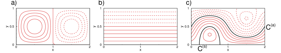
Figure 1: Reference streamfunction fields with solid and broken lines for positive and negative contour values: a) principal Rossby wave; b) eastward jet; and c) total for a supercritical case with $a_{(0)}=0.5$. Two thick lines in c are the kinematically defined boundary curves used in this study: a periodic orbit $C^{{\rm(a)}}$ corresponding to the jet axis with period $T^{(a)}=1.260549$; a separatrix $C^{{\rm(u)}}$ dividing the southern anti-cyclonic recirculating cell from the eastward jet. The trough and ridges of the reference flow are at $x=1/2$ and $3/2$, respectively.

satisfies the steady state condition of the dynamic quasi-geostrophic (QG) model for large-scale planetary flows, $\frac{\partial{}}{\partial{t}}{\bar{q}}({\bf{x}},t)=0$, where ${\bar{q}}({\bf{x}})=\nabla_{{\bf{x}}}^{2}{\bar{\psi}}({\bf{x}})+y$ is the potential vorticity of the reference flow. The first term of the right-hand side is the principal Rossby wave with amplitude $a_{(0)}$ and wave-number vector $(1,1)$ in ${\bf{x}}$, which consists of the upstream anti-cyclonic and downstream cyclonic recirculating cells (Figure 1a). The second term is a uniform jet induced by moving with the principal Rossby wave relative to the earth-fixed frame at a constant phase speed $1$ (Figure 1b). The geometry of the reference flow (8) bifurcates as the amplitude $a_{(0)}$ varies. In this study, we consider a case where the flow is supercritical, i.e., $1>a_{(0)}>{1}/{\pi}$, so that it corresponds to a blocked state of the atmospheric jet over topography (Charney & De Vore, 1979). If the flow field is given by a numerical simulation of the QG model, then the time average of $\psi({\bf{x}},t)$ can be used as ${\bar{\psi}}({\bf{x}})$. In a blocked flow, the two separatrices divide the reference flow field into three kinematically distinct regions: a pair of upstream and downstream recirculation cells and an eastward jet (Figure 1c). The jet flows faster where it makes turns at the trough $(x=1/2)$ and ridge $(x=3/2)$ to pass the recirculating cells.

In this kinematic model, $N$ additional Rossby traveling waves  comprise the anomaly field $\psi^{\prime}({\bf{x}},t)=\sum_{n=1}^{N}\psi_{(n)}({\bf{x}},t)$, where the $n$-th wave

$$\psi_{(n)}({\bf{x}},t) = \epsilon_{(n)}\sin[k_{(n)}\pi(x-b_{(n)}t)]\sin(l_{(n)}\pi y)~{}:$$ (9)

is defined by amplitude $\epsilon_{(n)}$ and wave-number vector $(k_{(n)},l_{(n)})$ for $k_{(n)}l_{(n)}>1$. Because a Rossby wave with a higher wave number travels faster, the phase speed $b_{(n)}\equiv 1-{2}/({k_{(n)}^{2}+l_{(n)}^{2}})$ is positive. Throughout the paper, the subscript in parentheses represents the identity of the Rossby traveling wave. Table 1 summarizes the five additional Rossby traveling waves used in this study. For comparison purposes, we fix the amplitude $\epsilon_{(n)}=0.1$ for all $n$.

Based on the spatio-temporal decomposition (Section 1.1), the $n$-th Rossby traveling wave is made up by a pair $[2n-1,2n]$, i.e., $\psi_{(n)}({\bf{x}},t)\equiv\tilde{\psi}_{[2n-1,2n]}({\bf{x}},t)$, where the notation convention for the pair follows (5). The variance, spatial PC, and temporal PC of $\tilde{\psi}_{2n-1}({\bf{x}},t)$ and $\tilde{\psi}_{2n}({\bf{x}},t)$ corresponding to (3) can be defined as:

$$\begin{array}[]{lllclrr}(\sigma_{2n-1},&\psi_{2n-1}({\bf{x}}),&f_{2n-1}(t))&=&(\epsilon_{(n)},&\sin(k_{(n)}\pi x)\sin(l_{(n)}\pi y),&\cos(k_{(n)}b_{(n)}\pi t)~{})~{},\\ (\sigma_{2n},&\psi_{2n}({\bf{x}}),&f_{2n}(t))&=&(\epsilon_{(n)},&-\cos(k_{(n)}\pi x)\sin(l_{(n)}\pi y),&\sin(k_{(n)}b_{(n)}\pi t)~{})~{}.\end{array}$$ (12)

In the spectral representation of the dynamic QG model, $\sigma_{i}f_{i}(t)$ can be thought of as the residual of the spectral coefficients for pre-selected $psi_{i}({\bf{x}})$.

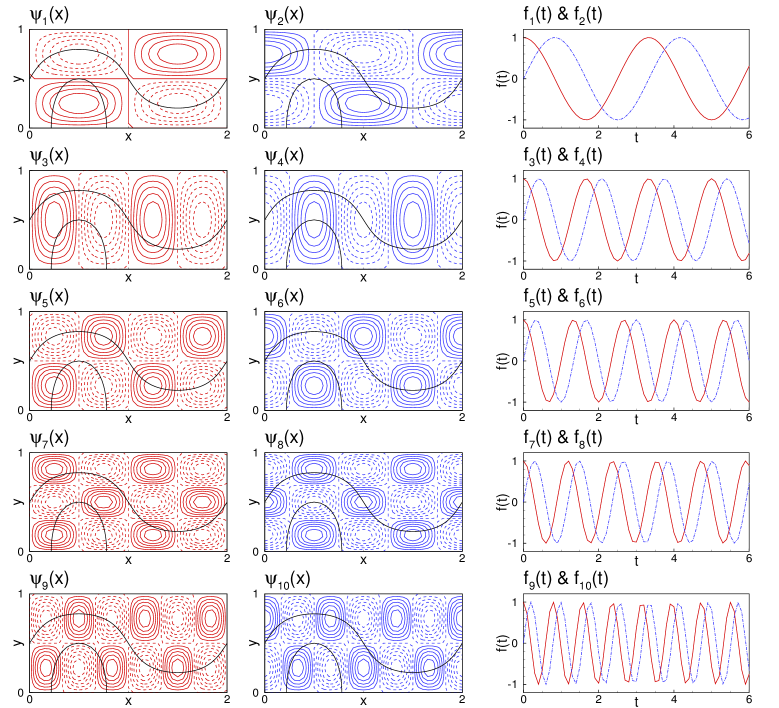
Figure 2: Spatial and temporal components of the dynamical modes corresponding to the five Rossby traveling waves (see Table 1). The left and center panels are $\psi_{2n-1}({\bf{x}})$ and $\psi_{2n}({\bf{x}})$, respectively, where solid and dashed lines represent positive and negative contour values with contour interval 0.2. The two boundary curves $C^{{\rm(a)}}$ and $C^{{\rm(u)}}$ are also shown by the solid curves. The right panels are $f_{2n-1}(t)$ and $f_{2n}(t)$ in solid and dashed lines, respectively.

Variability of this model has the properties commonly observed in large-scale planetary flows as discussed in Section 1.1, if we choose $\epsilon_{(n)}\geq\epsilon_{({n+1})}$, $k_{(n)}\leq k_{({n+1})}$, and $l_{(n)}\leq l_{({n+1})}$ with $k_{(n)}l_{(n)}<k_{({n+1})}l_{({n+1})}$. The spatial PCs of pair $[2n-1,2n]$ have $l_{(n)}$ latitudinal lines along which $2k_{(n)}$ dynamic eddies align (Figure 2). The characteristic length-scale is $L^{({\bf{u}})}_{2n-1}={1}/{k_{(n)}}$ along the dynamic alignment curve. The temporal PCs have the characteristic time-scale $T^{({\bf{u}})}_{2n-1}=1/(k_{(n)}b_{(n)})$. Pair by pair, $L^{({\bf{u}})}_{2n-1}$ and $T^{({\bf{u}})}_{2n-1}$ decreases as $k_{(n)}l_{(n)}$ increases.

Because the coherent evolution of dynamic eddies is essential in understanding the role of variability in transport, we briefly demonstrate how a pair generates a Rossby traveling wave by following Section 1.1. The spatial PC of the first dynamic mode $2n-1$ has $l_{(n)}$ sets of $2N^{({\bf{u}})}_{2n-1}=2k_{(n)}$ dynamic eddies (left panels of Figure 2) which alternate in sign along the dynamic alignment curves $y=(j-\frac{1}{2})/l_{(n)}$ for $j=1,\ldots,l_{(n)}$. The spatial PC of the second dynamic mode $2n$ also has $l_{(n)}$ sets of $2N^{({\bf{u}})}_{2n-1}$ dynamic eddies along the same curves (middle panels of Figure 2). The two spatial PCs have the centers of the dynamic eddies staggered with respect to each other along the alignment curves, while their corresponding temporal PCs satisfy (4) and (6). The four phases of $\tilde{\psi}_{{[2n-1,2n]}}({\bf{x}},t)$ over one recurrent cycle $2T^{({\bf{u}})}_{2n-1}$ are $\psi_{2n-1}({\bf{x}})$, $\psi_{2n}({\bf{x}})$, $-\psi_{2n-1}({\bf{x}})$, and $-\psi_{2n}({\bf{x}})$ in a time sequence (Figure 2). In summary, $\tilde{\psi}_{[2n-1,2n]}({\bf{x}},t)$ has $l_{(n)}$ sets of $N^{({\bf{u}})}_{2n-1}$ positive and $N^{({\bf{u}})}_{2n-1}$ negative dynamic eddies that propagate straight eastward with the positive phase speed $b^{({\bf{u}})}_{{[2n-1,2n]}}=L^{({\bf{u}})}_{2n-1}/T^{({\bf{u}})}_{2n-1}=b_{(n)}$.

It is worth noting the case where the spatial PCs of a pair have an opposite phase relation, i.e., $\psi_{2n-1}(x,y)=\psi_{2n}(x-{L^{({\bf{u}})}_{2n-1}}/{2},y)$ instead of $\psi_{2n-1}(x,y)=\psi_{2n}(x+{L^{({\bf{u}})}_{2n-1}}/{2},y)$ as in (12). In $\tilde{\psi}_{[2n-1,2n]}({\bf{x}},t)$, $l_{(n)}$ sets of $2N^{({\bf{u}})}_{2n-1}$ dynamic eddies would advect in the reverse direction with a negative constant phase speed $-b^{({\bf{u}})}_{{[2n-1,2n]}}$ along the same curves. This artificial setting could happen if a Rossby traveling wave with smaller length-scale travels slower in the earth-fixed frame.

3 Basics of TIME

We briefly present basic ideas and formulae of the TIME used in later sections. The mathematical derivations and a detailed discussion can be found in Ide & Wiggins (2014b, a).

3.1 Boundary of transport

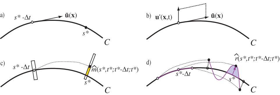
Figure 3: Geometry associated with the TIME: a) boundary curve $C$ and particle motion in the steady reference flow; b) instantaneous flux across $C$ in the unsteady flow; c) fluid column evolution in the unsteady flow and accumulation of flow property; d) geometry of particle transport $C$ and pseudo-lobe defined by $R$ and $C$.

In TIME, we evaluate transport across a stationary boundary defined by a reference streamline ${\bar{\chi}}({\bf{x}})$ of our choice. We denote this boundary curve by $C$. To present the theory using the geometric approach of dynamical systems, we define two coordinate variables along $C=\{{\bar{\bf{x}}}^{C}(s)\}$. Here $s$ is the flight-time coordinate in a unit of time so that a fluid particle starting from ${\bar{\bf{x}}}^{C}(s^{*}-\triangle t)$ reaches ${\bar{\bf{x}}}^{C}(s^{*})$ after a time interval $\triangle t$ in the reference flow (Figure 3a). By this definition, $s$ satisfies $\frac{d{}}{d{s}}{\bar{\bf{x}}}^{C}(s)={\bar{{\bf{u}}}}({\bar{\bf{x}}}^{C}(s))$ and any particle travels with a non-dimensional phase speed $\frac{d{}}{d{t}}s=1$.

We denote the upstream and downstream end points of $C$ by $s_{-}$ and $s_{+}$, respectively. The length of $C$ measured in a unit of (flight) time depends on the kinematic type of $C$ as follows. If $C$ is an unstable or stable invariant manifold associated with a DHT (i.e., a hyperbolic stagnation point in the reference flow), then it has a semi-infinite length with $s_{-}\to-\infty$ or $s_{+}\to\infty$ towards the direction of the DHT. If $C$ is a separatrix along which an unstable and stable invariant manifold coincide, then it has a bi-infinite length. If $C$ has no DHT at either end point, then it has a finite length. Using an example (Figure 1), this study demonstrates our method across two types of $C$: an infinite length along the upstream separatrix $C^{{\rm(u)}}$ between the jet and the recirculating cell, and a finite length along the jet axis $C^{{\rm(a)}}$ between the northern and southern parts of the jet.

Arc-length $l=l^{C}(s)$ is another coordinate variable along $C$ corresponding to the arc-length distance traveled by a particle. The geometry of TIME can be naturally described using $l$ because it has a unit of length. The two coordinate variables are related by the local velocity, i.e., $\frac{d{}}{d{s}}l^{C}(s)=|{\bar{{\bf{u}}}}({\bar{\bf{x}}}^{C}(s))|$. From here on, we let $(s,t)$ and $(l^{C}(s),t)$ represent the combination of a position ${\bar{\bf{x}}}^{C}(s)$ along $C$ at a time $t$.

3.2 Mechanism of TIME

In an unsteady flow, a component of instantaneous velocity normal to $C$ repels particles away from $C$. The instantaneous flux normal to $C$ at $(s,t)$

$$\tilde{\mu}^{C}(s,t) \equiv {\bar{{\bf{u}}}}({\bar{\bf{x}}}^{C}(s))\wedge{\bf{u}}^{\prime}({\bar{\bf{x}}}^{C}(s),t)~{}:$$ (13)

is the signed area of the parallelogram defined by ${\bar{{\bf{u}}}}({\bar{\bf{x}}}^{C}(s))$ and ${\bf{u}}^{\prime}({\bar{\bf{x}}}^{C}(s),t)$ (Figure 3b), where “$\wedge$” denotes the normal wedge product. For $\tilde{\mu}^{C}(s,t)>0$, the instantaneous flux is from right to left across $C$ with respect to the forward direction of the reference flow. The direction of the flux reverses for $\tilde{\mu}^{C}(s,t)<0$.

There are two approaches to the TIME. One considers the net transport of the flow property $q$ defined in (1b). This is pursued by accumulating instantaneous flux while advecting with the flow. Another approach determines the geometry associated with particle transport. This is pursued by computing the displacement distance of a particle originally placed on $C$. In the special case of mass transport with $q=1$ in an incompressible flow, the two approaches lead to the same formula.

We illustrate the first approach using a fluid column that originally intersects with $C$ at $(s^{*}-\triangle t,t^{*}-\triangle t)$ (marked by a white circle in Figure 3c). If the flow is steady, then that original intersection remains on $C$ at $(s^{*}-t^{*}+\tau,\tau)$ for $t^{*}-\triangle t<\tau<t^{*}$ and reaches $(s^{*},t^{*})$ after a time interval $\triangle t$. In the unsteady flow, the original intersection moves away from $C$ due to the component of ${\bf{u}}^{\prime}({\bf{x}},t)$ normal to $C$ (marked by a dark circle). The displaced portion of the column (marked by a shaded area) stores continuously accumulating instantaneous flux of $q$ across $C$. This accumulation of $q$ is the TIME we wish to compute. It can be shown that the net accumulation of $q$ in the column over the time interval is:

$$\hat{m}(s^{*},t^{*};t^{*}-\triangle t:t^{*})=\int_{t^{*}-\triangle t}^{t^{*}}{\bar{q}}({\bar{\bf{x}}}^{C}(s^{*}-t^{*}+\tau))\tilde{\mu}^{C}(s^{*}-t+^{*}\tau,\tau)d\tau~{},$$ (14)

up to the leading order, where the integrand is instantaneous flux of $q$ at $(s^{*}-t^{*}+\tau,\tau)$ for $\tau\in[t^{*}-\triangle t,t^{*}]$.

In the illustration above, TIME is evaluated over the time interval just past the evaluation time $t^{*}$. A straightforward extension of (14) gives the TIME of $q$ evaluated at an arbitrary $(s,t)$ that occurs over a spatial segment $[s_{a},b_{b}]$ during a time interval $[t_{0},t_{1}]$:

$$m^{C}(s,t;s_{a}:s_{b},t_{0}:t_{1})=\int_{t_{0}}^{t_{1}}H(s-t+\tau;s_{a}:s_{b})\tilde{\mu}^{C,q}(s-t+\tau,\tau)d\tau~{},$$ (15)

where $\tilde{\mu}^{C,q}(s,t)\equiv{\bar{q}}({\bar{\bf{x}}}^{C}(s))\mu^{C}(s,t)$. The two limits of the integral specify the temporal interval and

$$H(\theta;s_{a}:s_{b})=\left\{\begin{array}[]{ll}1&\mbox{ for $s_{a}\leq\theta\leq s_{b}$},\\ 0&\mbox{ otherwise}~{}:\end{array}\right.$$ (18)

takes care of the spatial segment. The sign of $m^{C}(s,t;s_{a}:s_{b},t_{0}:t_{1})$ shows the direction of TIME: a positive sign corresponds to accumulation of $q$ from the right to left region across $C$ (with respect to the forward direction of the reference flow). The directions reverse for the negative sign. We call $m^{C}(s,t;s_{a}:s_{b},t_{0}:t_{1})$ the “accumulation function,” where the two sets of arguments $(s,t)$ and $(s_{a}:s_{b},t_{0}:t_{1})$ are the “evaluation point and time” and “domain of integration,” respectively.

We illustrate the second approach for the geometry associated with particle transport using a material line $R$ initially placed along $C$ at time $t^{*}-\triangle t$ (Figure 3d). In the unsteady flow, the normal component of the unsteady velocity displaces $R$ from $C$. The deformed $R$ and stationary $C$ form structures called “pseudo-lobes” which show the local coherency of TIME. The prefatory word “pseudo” is used to distinguish from its counterpart in Lagrangian lobe dynamics. In Figure 3d, the shaded area surrounded by $R$ and $C$ is a pseudo-lobe of TIME over the immediate past time interval $\triangle t$. The arrow at $(s^{*},t^{*})$ is the corresponding signed distance $\hat{r}(s^{*},t^{*};t^{*}-\triangle t:t^{*})$. In general, the “displacement distance” function for the signed normal distance from $C$ to $R$ can be written as:

$$r^{C}(l^{C}(s),t;s_{a}:s_{b},t_{0}:t_{1}) = {a^{C}(s,t;s_{a}:s_{b},t_{0}:t_{1})}/{||{\bar{{\bf{u}}}}({\bar{\bf{x}}}^{C}(s))||}~{},$$ (19a)

where

$$a^{C}(s,t;s_{a}:s_{b},t_{0}:t_{1}) = e(s:s_{a})\int_{t_{0}}^{t_{1}}H(s-t+\tau;s_{a}:s_{b})\tilde{\mu}^{C,e}(s-t+\tau,\tau)d\tau~{}:$$ (19b)

is the so-called “displacement area” function having a unit of area per (flight) time and taking the compressibility of the reference flow into account:

$$e(s:s_{a}) = \exp\left\{\int_{s}^{s_{a}}J[{\bar{{\bf{u}}}},{\bf{x}}]({\bar{\bf{x}}}^{C}(\theta))d\theta\right\}~{},$$ (20)

and $\tilde{\mu}^{C,e}(s,t)\equiv e(s_{a}:s)\tilde{\mu}^{C}(s,t)$. The convention of the arguments follows that of $m^{C}(s,t;s_{a}:s_{b},t_{0}:t_{1})$, but $l^{C}(s)$ replaces $s$ for the distance function (19a) to describe the transport geometry in a physically consistent unit of length along $C$. The sign of the displacement functions represents the transport direction, as in the accumulation function.

When the displacement functions are applied to a separatrix with the infinite domain of integration in both $s$ and $t$, $a^{C}(s,t;-\infty:\infty,-\infty:\infty)$ coincides with the so-called “Melnikov function” used in Lagrangian lobe dynamics. Accompanying $r^{C}(l^{C}(s),t;-\infty:\infty,-\infty:\infty)$ can be interpreted as the leading order approximation of the signed distance from the stable to unstable invariant manifolds measured at $(s,t)$ normal to $C$.

We call the accumulation and displacement functions in (15) and (19) collectively the “TIME functions.” They can be evaluated at any point and time in the $(s,t)$ space, and represent the amount of transport that has occurred, is occurring, or will occur, depending on the relative relation of $(s,t)$ to $(s_{a}:s_{b},t_{0}:t_{1})$. We define two categories of TIME relevant to large-scale geophysical flows as follows. “Definite” TIME measures the net amount of transport for a fixed $(s_{a}:s_{b},t_{0}:t_{1})$ which can extend to $(-\infty:\infty,-\infty:\infty)$ if $C$ is a separatrix, as above. In contrast, “Finite-time” TIME measures transport over the immediate past time interval starting at time $t^{\dagger}$ up to the present $t$, i.e., the domain of integration $(s^{\dagger}:s,t^{\dagger}:t)$ varies as $t$ progresses.

3.3 Spatial coherency and temporal evolution

Using, for simplicity, the displacement area function $a^{C}(s,t)=a^{C}(s,t:s_{a}:s_{b},t_{0}:t_{1})$ related to particle transport, we describe the spatial coherency of TIME based on the geometry of pseudo-lobes at $t$ and the temporal evolution based on the phase speed and deformation in $t$. For simplicity of notation, we drop the argument for the domain of integration. It is straightforward to extend this discussion for TIME of a flow property $q$ by replacing $a^{C}(s,t)$ with $m^{C}(s,t)$. We drop the arguments corresponding to the domain of integration for notational convenience.

We start from spatial coherency at time $t$. The zero sequence $\{s^{C}_{j}(t)\}$ of $a^{C}(s,t)$ defined by

$$a^{C}(s^{C}_{j}(t),t) = 0~{}:$$ (21)

is the ordered intersection sequence of $R$ with $C$ from upstream to downstream (Figure 3), because the zeros of $a^{C}(s,t)$ and $r^{C}(l^{C}(s),t)$ have one-to-one correspondence from (19a). We call $\{s^{C}_{j}(t)\}$ the “pseudo-PIP” sequence.

The definition of the “pseudo-lobe” ${\cal L}^{C}_{j:j+1}(t)$ follows naturally in the $(s,a)$ coordinate as the region defined by the two curves, $a=a^{C}(s,t)$ for $R$ and $a=0$ for $C$, over the segment between the two adjacent pseudo-PIPs, $s\in[s^{C}_{j}(t),s^{C}_{j+1}(t)]$. The sign of $a^{C}(s,t)$ normally alternates pseudo-lobe by pseudo-lobe along $C$: a positive pseudo-lobe with $a^{C}(s,t)>0$ lies on the left of $C$ and represents local coherency of TIME from the right across $C$. The directions are reversed for a negative pseudo-lobe. The definition of ${\cal L}^{C}_{j:j+1}(t)$ can be extended into the $(l,r)$ space, which can in turn be projected into the ${\bf{x}}$ space along $C$. Given $a^{C}(s,t)$, the signed area of ${\cal L}^{C}_{j:j+1}(t)$ is:

$$A^{C}_{j:j+1}(t) \equiv \int_{l^{C}(s^{C}_{j}(t))}^{l^{C}(s^{C}_{j+1}(t))}r^{C}(l,t)dl=\int_{s^{C}_{j}(t)}^{s^{C}_{j+1}(t)}a^{C}(s,t)ds~{}.$$ (22)

In the $(s,a)$ space, spatial coherency of TIME is described by the geometry of ${\cal L}^{C}_{j:j+1}(t)$, i.e., the separation distance of pseudo-PIPs $\triangle s^{C}_{j:j+1}(t)\equiv s^{C}_{j+1}(t)-s^{C}_{j}(t)$ and average height $\check{a}^{C}_{j:j+1}(t)\equiv A^{C}_{j:j+1}(t)/\triangle s^{C}_{j:j+1}(t)$. The latter also measures transport efficiency of ${\cal L}^{C}_{j:j+1}(t)$ in a unit of area per time. Naturally, temporal evolution can be described by the phase speed $\frac{d{}}{d{t}}s^{C}_{j}(t)$ for propagation, and change of $A^{C}_{j:j+1}(t)$ for deformation. In the $(l,r)$ and ${\bf{x}}$ spaces, the geometry of ${\cal L}^{C}_{j:j+1}(t)$ can be significantly distorted if ${\bar{{\bf{u}}}}({\bar{\bf{x}}}^{C}(s))\approx 0$. The effect is most apparent along a separatrix near the DHT.

4 Variability in instantaneous flux

In a series of steps, we build a framework to identify the signature of dynamic variability in transport.

4.1 Global instantaneous flux

We begin by globally examining the instantaneous flux field in ${\bf{x}}$:

$$\phi({\bf{x}},t) \equiv {\bar{{\bf{u}}}}({\bf{x}})\wedge{\bf{u}}^{\prime}({\bf{x}},t).$$ (23a)

Using the spatio-temporal decomposition of dynamic variability (3), the “flux variability” is:

$$\tilde{\phi}_{i}({\bf{x}},t) \equiv {\bar{{\bf{u}}}}({\bf{x}})\wedge\tilde{{\bf{u}}}_{i}({\bf{x}},t)=\sigma_{i}\phi_{i}({\bf{x}})f_{i}(t)~{},$$ (23b)

for mode $$i \tilde{\phi}_{[i,i+1]}({\bf{x}},t)\equiv\tilde{\phi}_{i}({\bf{x}},t)+\tilde{\phi}_{i+1}({\bf{x}},t) [i,i+1] \phi({\bf{x}},t)$$ and for pair . The total instantaneous flux field is a linear sum of contributions from all modes and noise.

An expected, yet striking feature of (23b), is that flux variability preserves the temporal PCs of the dynamic variability. This is because the reference flow ${\bar{{\bf{u}}}}({\bf{x}})$ has no temporal component to interact with $\tilde{{\bf{u}}}_{i}({\bf{x}},t)$. The temporal signature of dynamic variability is carried into the flux variability as the characteristic time-scale $T^{({\bf{u}})}_{i}$. In contrast, the spatial component of the flux mode

$$\phi_{i}({\bf{x}}) \equiv {\bar{{\bf{u}}}}({\bf{x}})\wedge{\bf{u}}_{i}({\bf{x}})~{}:$$ (23c)

is the result of the nonlinear interaction between the dynamic variability and the reference flow. If the flow is incompressible, then it leads to a geometric representation using the streamfunction, i.e., $\phi_{i}({\bf{x}})=-J[{\bar{\psi}}({\bf{x}}),\psi_{i}({\bf{x}})]$. Locally at ${\bf{x}}$, $\phi_{i}({\bf{x}})$ is the signed area of the parallelogram defined by ${\bar{{\bf{u}}}}({\bf{x}})$ and ${\bf{u}}_{i}({\bf{x}})$ (see also Figure 3c). Globally, it may have coherent structures which we call “flux eddies.” A positive flux eddy represents local coherency of the instantaneous flux from right to left across the reference streamline. The direction of the flux reverses for a negative flux eddy. We define the characteristic length-scale $L^{(\phi)}_{i}$ of $\phi_{i}({\bf{x}})$ by the typical width of the flux eddies.

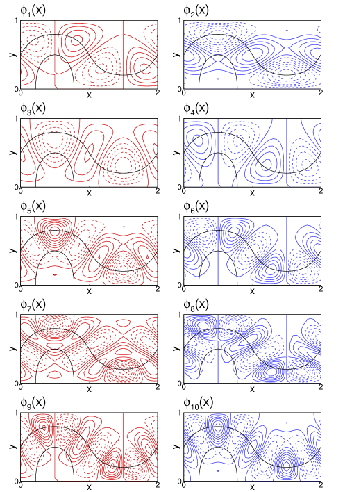
Figure 4: Spatial components $\phi_{i}({\bf{x}})$ of the flux mode corresponding to Figure 2 , where solid and dashed lines represent positive and negative contour values with contour interval 1.

The spatial signatures of dynamic variability in $\phi_{i}({\bf{x}})$ can be found in the nonlinear generation of flux eddies from the interaction of dynamic eddies and the reference flow. The amplitude of ${\bar{{\bf{u}}}}({\bf{x}})$, ${\bf{u}}_{i}({\bf{x}})$, and angle between them define the spatially nonlinear interaction (23c). Hence flux eddies tend to form where ${\bar{{\bf{u}}}}({\bf{x}})$ is swift and the dynamic eddies concentrate. The center of a dynamic eddy should be near the edge of a flux eddy because $|{\bf{u}}_{i}({\bf{x}})|=0$ and hence $\phi_{i}({\bf{x}})=0$ there (compare Figure 4 with Figure 2). Conversely, the center of a flux eddy may be located between two adjacent dynamic eddies because $|{\bf{u}}_{i}({\bf{x}})|$ may be large there. As a result, flux eddies tend to stagger with respect to dynamic eddies in a nonlinear way. They may not distribute homogeneously even where dynamic eddies do. Due to the spatially nonlinear interaction, $L^{(\phi)}_{i}$ and $L^{({\bf{u}})}_{i}$ can be different.

Using the atmospheric model, we demonstrate the nonlinear generation of flux eddies. Because the reference flow is swift along the jet axis and dynamic eddies distribute homogeneously everywhere, all significant flux eddies emerge along the reference jet only. The flux eddies may distribute inhomogeneously even along the jet: strong flux eddies lie near the ridge and trough where the jet flows fastest. For the $n$-th Rossby traveling wave, both $\phi_{2n-1}({\bf{x}})$ and $\phi_{2n}({\bf{x}})$ have $N^{(\phi)}_{2n-1}$ positive and $N^{(\phi)}_{2n-1}$ negative flux eddies (Table 1). The two strong flux eddies at the ridge and trough have the same sign unless the wave numbers $(k_{(n)},l_{(n)})$ are both even. Because $2N^{(\phi)}_{2n-1}$ flux eddies emerge as the jet cuts across $l_{(n)}$ horizontal lines of $2N^{({\bf{u}})}_{2n-1}$ dynamic eddies, Flux eddies outnumber dynamical eddies per respective alignment curve, i.e., $2N^{(\phi)}_{2n-1}>2N^{({\bf{u}})}_{2n-1}$ for $l_{(n)}>1$. Thus, the characteristic length-scale $L^{(\phi)}_{2n-1}=1/N^{(\phi)}_{2n-1}$ is smaller than $L^{({\bf{u}})}_{2n-1}=1/N^{({\bf{u}})}_{2n-1}$.

Having understood the spatial features in $\phi_{i}({\bf{x}})$ and $\phi_{i+1}({\bf{x}})$, we now describe the evolution of flux eddies in the spatio-temporal decomposition $\tilde{\phi}_{i}({\bf{x}},t)$ and $\tilde{\phi}_{[i,i+1]}({\bf{x}},t)$. The temporal PCs $f_{i}(t)$ and $f_{i+1}(t)$ satisfy the phase conditions (4) and (6). As a single mode, $\tilde{\phi}_{i}({\bf{x}},t)$ is a geometric pattern that pulsates with the same recurrent cycle $2T^{({\bf{u}})}_{i}$ as $\tilde{\chi}_{i}({\bf{x}},t)$. As a pair $[i,i+1]$, $\tilde{\phi}_{[i,i+1]}({\bf{x}},t)$ has some ‘flux alignment curves” along which flux eddies undergo recurrent evolution. The four phases of $\tilde{\phi}_{[i,i+1]}({\bf{x}},t)$ at every ${T^{({\bf{u}})}_{i}}/{2}$ are $\phi_{i}({\bf{x}})$, $\phi_{i+1}({\bf{x}})$, $-\phi_{i}({\bf{x}})$, and $-\phi_{i+1}({\bf{x}})$ over one recurrent cycle $2T^{({\bf{u}})}_{i}$ (Figure 4). The flux phase speed $b^{(\phi)}_{[i,i+1]}$ is $L^{(\phi)}_{i}/T^{({\bf{u}})}_{i}$. Because of the spatially nonlinear interaction, the evolution of flux and dynamic eddies may not exhibit a one-to-one correspondence, except for the same recurrent cycle: their alignment curves and respective phase speeds can differ.

In the atmospheric model, any $\tilde{\phi}_{i}({\bf{x}},t)$ has $2N^{(\phi)}_{i}$ flux eddies that pulsate with the recurrent cycle $2T^{({\bf{u}})}_{i}$. As the $n$-th Rossby traveling wave travels straight eastward along $l_{(n)}$ lines, it generates $N^{(\phi)}_{2n-1}$ positive and $N^{(\phi)}_{2n-1}$ negative flux eddies that propagate eastward along the reference jet in $\tilde{\phi}_{[2n-1,2n]}({\bf{x}},t)$. The flux eddies have a phase speed $b^{(\phi)}_{[2n-1,2n]}=L^{(\phi)}_{2n-1}/T^{({\bf{u}})}_{2n-1}$, which is smaller than $b^{({\bf{u}})}_{[2n-1,2n]}$ of the dynamic eddies by a factor $N^{({\bf{u}})}_{2n-1}/N^{(\phi)}_{2n-1}$ for $l_{(n)}>1$. Two flux eddies pass the ridge and trough synchronously when their amplitude reaches maximum. The sign of the two is the same, unless both wave numbers $(k_{(n)},l_{(n)})$ are even. Strikingly, these Rossby traveling waves inducing instantaneous flux near the meandering jet but not so much in the recirculation cells, despite traveling homogeneously throughout the flow domain.

It is worth mentioning the additional case discussed in Section 2 where the pair’s spatial PCs have an opposite phase relation. Then, the flux eddies in $\tilde{\phi}_{[2n-1,2n]}({\bf{x}},t)$ would propagate in the reverse direction with a negative constant phase speed $-b^{(\phi)}_{[2n-1,2n]}$ along the flux alignment curve.

4.2 Instantaneous flux across $C$

The most basic element of the TIME functions is the instantaneous flux $\tilde{\mu}^{C}(s,t)$ across $C$ as in (15) and (19). Using $\tilde{\phi}_{i}({\bf{x}},t)$, we identify the signature of dynamic variability in $\tilde{\mu}^{C}_{i}(s,t)$. Applying (3) to (13) and using

(23b) give:

$$\tilde{\mu}^{C}_{i}(s,t) \equiv\sigma_{i}\mu^{C}_{i}(s)f_{i}(t)~{}.$$ (24a)

The temporal component $$f_{i}(t) \tilde{{\bf{u}}}_{i}({\bf{x}},t)$$ directly relates to the dynamic variability . The spatial component

$$\mu^{C}_{i}(s)=\phi_{i}({\bar{\bf{x}}}^{C}(s))~{}:$$ (24b)

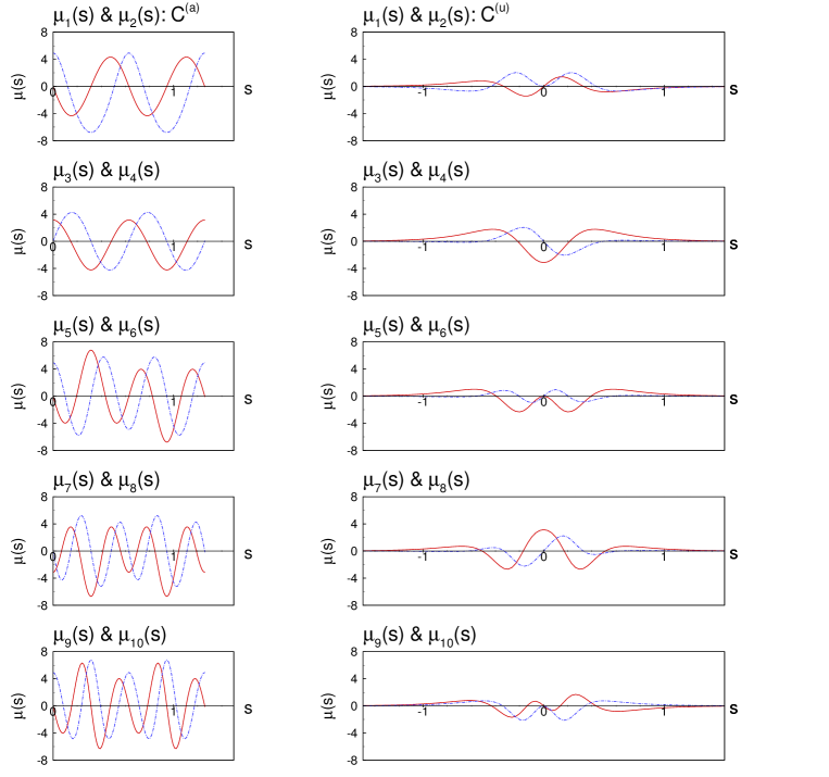
Figure 5: Spatial component $\mu^{C}_{i}(s)$ of flux mode along $C^{{\rm(a)}}$ (left panels) and $C^{{\rm(u)}}$ (right panels) corresponding to Figure 4, where solid and dashed lines are for $\mu^{C}_{2n-1}(s)$ and $\mu^{C}_{2n}(s)$, respectively. In the left panels, $s=0.3157$ and $0.9454$ correspond to the two turning points of $C^{{\rm(a)}}$ at $x=1/2$ and $3/2$ over the trough and ridge. In the right panels, $s=0$ corresponds to the trough along $C^{{\rm(u)}}$. All flux eddies of $\mu^{{\rm(u)}}_{i}(s)$ concentrate over the segment $s\in[-1,1]$ where ${\bar{\bf{x}}}^{{\rm(u)}}(-1)$ and ${\bar{\bf{x}}}^{{\rm(u)}}(1)$ are near the upstream and downstream DHTs ${\bar{\bf{x}}}^{{\rm(u)}}(-\infty)$ and ${\bar{\bf{x}}}^{{\rm(u)}}(\infty)$ in the ${\bf{x}}$ space, respectively.

is extracted from the global mode $\phi_{i}({\bf{x}})$ in terms of flux eddies along $C$ (e.g., Figure 4). Over a positive flux eddy, $\mu^{C}_{i}(s)>0$ represents local coherency of instantaneous flux from right to left across $C$. The sign and direction reverse over a negative flux eddy. Therefore, the dynamic roots of $\mu^{C}_{i}(s)$ (Figure 5) can be traced back to dynamic eddies in $\chi_{i}({\bf{x}})$ (Figure 2) through flux eddies in $\phi_{i}({\bf{x}})$ (Figure 4). The characteristic length-scale $S^{C}_{i}$ of $\mu^{C}_{i}(s)$ is defined by typical width of flux eddies in a unit of flight time by a reference trajectory along $C$. Given $\phi_{i}({\bf{x}})$, $\mu^{C}_{i}(s)$ depends critically on $C$ as shown for $C^{{\rm(a)}}$ and $C^{{\rm(u)}}$ of the atmospheric model in Figure 5 . The two main controlling factors for $C$ are listed below. $C$ may consist of more than one segment with different factors.

1. Geographic location.

   The geographic location of $C$ with respect to flux eddies can lead to the spatial phase conditions for $\mu^{C}_{i}(s)$ and $\mu^{C}_{i+1}(s)$: counterparts of the temporal phase conditions for $f_{i}(t)$ and $f_{i+1}(t)$ as in (4) and (6).

   For a single mode $i$, if $C$ goes through the middle of flux eddies in $\phi_{i}({\bf{x}})$, then $\mu^{C}_{i}(s)$ may be regular and have the spatial phase condition:

   $$\mu^{C}_{i}(s) \approx -\mu^{C}_{i}(s+S^{C}_{i})~{}.$$ (25)

   (left panels of Figure 5 in comparison with Figure 4). In contrast, if $C$ runs near the edge of the flux eddies, then $\mu^{C}_{i}(s)$ may be irregular (right panels of Figure 5).

   For a pair $[i,i+1]$, if $C$ goes along (a part of) a flux alignment curve, then $\mu^{C}_{i}(s)$ and $\mu^{C}_{i+1}(s)$ may be regular and have a similar structure over the segment. However, there is a phase shift between them due to the staggered centers of the flux eddies in $\phi_{i}({\bf{x}})$ and $\phi_{i+1}({\bf{x}})$. Such a phase shift can be one of the following:

   $$\mu^{C}_{i}(s) \approx \left\{\begin{array}[]{ll}\mu^{C}_{i+1}(s+\frac{S^{C}_{i}}{2})~{}:&\mbox{phase type (i)}~{},\\ \mu^{C}_{i+1}(s-\frac{S^{C}_{i}}{2})~{}:&\mbox{phase type (ii)}~{}.\end{array}\right.$$ (28)

   Phase type (i) corresponds to downstream propagation of the flux eddies in $\phi_{[i,i+1]}({\bf{x}},t)$ (Section 4.1). For the atmospheric model, all Rossby traveling waves belong to this type along $C^{{\rm(a)}}$ (left panels of Figure 5). For phase type (ii), the flux eddies propagate upstream against the reference flow, as for the additional case discussed in Sections 2 and 4.1. In contrast, if $C$ has little association with a flux alignment curve like $C^{{\rm(u)}}$ of the atmospheric model, then $\mu^{C}_{i}(s)$ and $\mu^{C}_{i+1}(s)$ are unlikely to satisfy either spatial phase conditions (28).

2. Kinematic type.

   If $C$ is either a semi- or bi-infinite boundary of transport associated with an invariant manifold or separatrix like $C^{{\rm(u)}}$ (Section 3), then $\mu^{C}_{i}(s)$ must decay exponentially to zero as $s$ approaches the corresponding DHT. Therefore, flux eddies must concentrate over some bounded segments of $s$ away from the DHT. In contrast, if $C$ has no DHT at the end points like $C^{{\rm(a)}}$, then the flux eddies may distribute along the entire segment of $C$, depending on the geographic location of $C$ with respect to flux eddies in $\phi_{i}({\bf{x}})$. If $C$ is a closed curve associated with a periodic orbit of period $T^{C}$, then $\mu^{C}_{i}(s)$ is also periodic.

Having described $\mu^{C}_{i}(s)$ and $\mu^{C}_{i+1}(s)$, we consider $\tilde{\mu}^{C}_{i}(s,t)$ and $\tilde{\mu}^{C}_{[i,i+1]}(s,t)$ as representative of evolving flux eddies extracted along $C$. As a single mode $i$, individual flux eddies act like stationary pistons that synchronously push flux across $C$. One push in each direction takes $T^{({\bf{u}})}_{i}$. The non-dimensional characteristic scale ratio for the flux eddies is:

$$\Gamma^{C}_{i} \equiv \frac{S^{C}_{i}}{T^{({\bf{u}})}_{i}}~{}.$$ (29)

As a pair, $\tilde{\mu}^{C}_{[i,i+1]}(s,t)$ significantly depends on the geographic location of $C$. If $C$ goes along (a part of) a flux alignment curve of phase type (i), then the flux eddies act like sliding pistons along $C$. Because they slide a distance $2S^{C}_{i}$ in a unit of flight time over $2T^{({\bf{u}})}_{i}$, the non-dimensional phase speed is $\Gamma^{C}_{i}$ in $\tilde{\mu}^{C}_{[i,i+1]}(s,t)$, which relates to dimensional phase speed $b^{(\phi)}_{[i,i+1]}$ in $\phi_{[i,i+1]}({\bf{x}},t)$. For phase type (ii), the non-dimensional phase speed is $-\Gamma^{C}_{i}$.

4.3 Spatio-temporal interaction

Having described $\tilde{\mu}^{C}_{i}(s,t)$ and $\tilde{\mu}^{C}_{[i,i+1]}(s,t)$, we identify the signature of dynamic variability in TIME using the graphical approach. Whenever possible, we use the subscript $\{\cdot\}_{\diamond}$ to represent mode $i$, $i+1$ or pair $[i,i+1]$ from here on. Using (15), (19) and (24), the corresponding TIME functions are:

$$m^{C}_{\diamond}(s,t;s_{a}:s_{b},t_{0}:t_{1}) = \int_{t_{0}}^{t_{1}}H(s-t+\tau;s_{a}:s_{b})\tilde{\mu}^{C,q}_{\diamond}(s-t+\tau,\tau)d\tau~{};$$ (30a)

$$a^{C}_{\diamond}(s,t;s_{a}:s_{b},t_{0}:t_{1}) = e(s:s_{a})\int_{t_{0}}^{t_{1}}H(s-t+\tau;s_{a}:s_{b})\tilde{\mu}^{C,e}_{\diamond}(s-t+\tau,\tau)d\tau~{},$$ (30b)

and $$r^{C}_{\diamond}(l^{C}(s),t;s_{a}:s_{b},t_{0}:t_{1})=a^{C}_{\diamond}(s,t;s_{a}:s_{b},t_{0}:t_{1})/||{\bar{{\bf{u}}}}({\bar{\bf{x}}}^{C}(s))||$$.

For simplicity, we focus on $a^{C}_{\diamond}(s,t;s_{a}:s_{b},t_{0}:t_{1})$ with $\tilde{\mu}^{C,e}_{\diamond}(s,t)=\tilde{\mu}^{C}_{\diamond}(s,t)$, which concerns incompressible particle transport. A full description of the TIME functions can be given by replacing $\tilde{\mu}^{C}_{\diamond}(s,t)$ with $\tilde{\mu}^{C,q}_{\diamond}(s,t)$ for flow property $q$, or by explicitly including $e(s_{a}:s)$ in $\tilde{\mu}^{C,e}_{\diamond}(s,t)$ for compressible particles. It is worth adding that $\tilde{\mu}^{C,q}_{\diamond}(s,t)$ and $\tilde{\mu}^{C,e}_{\diamond}(s,t)$ are roughly proportional to $\tilde{\mu}^{C}_{\diamond}(s,t)$ in large-scale planetary flows.

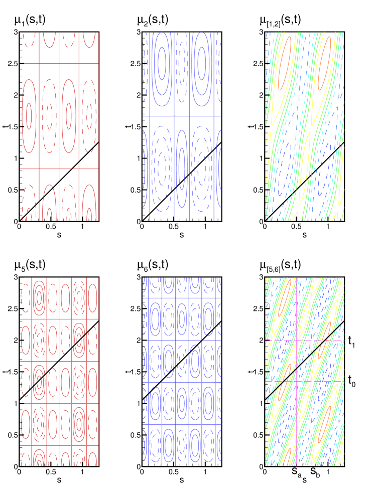
Figure 6: Instantaneous flux $\tilde{\mu}^{{\rm(a)}}(s,t)$ along $C^{{\rm(a)}}$ corresponding to Figures 4 and 5 where the solid and dashed lines are for positive and negative contour values with the contour interval 0.2; top panels are $\tilde{\mu}^{{\rm(a)}}_{{1}}(s,t)$, $\tilde{\mu}^{{\rm(a)}}_{{2}}(s,t)$, and $\tilde{\mu}^{{\rm(a)}}_{{[1,2]}}(s,t)$, and bottom panels are $\tilde{\mu}^{{\rm(a)}}_{{5}}(s,t)$, $\tilde{\mu}^{{\rm(a)}}_{{6}}(s,t)$, and $\tilde{\mu}^{{\rm(a)}}_{{[5,6]}}(s,t)$. An example for a diagonal line of integration $(s-t+\tau,\tau)$ going through $(0.625,1.675)$ is shown in each panel; an example for domain of integration $(s_{a}:s_{b},t_{0},t_{1})=(0.51:0.74,1.35:2)$ is shown in $\tilde{\mu}^{{\rm(a)}}_{{[5,6]}}(s,t)$.

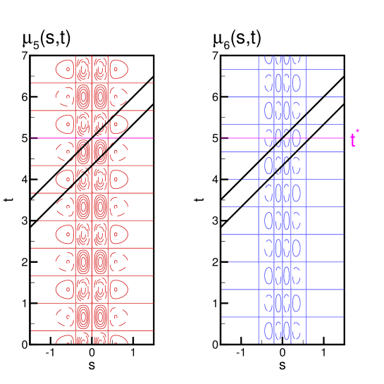
Figure 7: Instantaneous flux $\tilde{\mu}^{{\rm(u)}}_{{5}}(s,t)$ and $\tilde{\mu}^{{\rm(u)}}_{{6}}(s,t)$ for modes 5 and 6 along $C^{{\rm(u)}}$ corresponding to Instantaneous flux $\tilde{\mu}^{{\rm(u)}}_{{5}}(s,t)$ and $\tilde{\mu}^{{\rm(u)}}_{{6}}(s,t)$ for modes 5 and 6 along $C^{{\rm(u)}}$ corresponding to Figures 4 and 5 where the solid and dashed lines are for positive and negative contour values with the contour interval 0.05; Two example reference trajectories $(s-t+\tau,\tau)$ are separated by $T^{({\bf{u}})}_{{5}}$ in $s$ and $t$. An example evaluation time $t^{*}=5$ is also shown in the right panel.

The graphical approach examines the integration of $\tilde{\mu}^{C}_{\diamond}(s-t+\tau,\tau)$ along a reference trajectory $(s-t+\tau,\tau)$ (Figures 6, 7 and ). In the $(s,t)$ space, any reference trajectory is a diagonal line with the unit phase speed $\frac{d{}}{d{t}}s=1$. As a single mode, zero-$\tilde{\mu}^{C}_{\diamond}(s,t)$ contours divide the $(s,t)$ space vertically for flux eddies with width $S^{C}_{i}$, and horizontally for phases of $f_{i}(t)$ with interval $T^{({\bf{u}})}_{i}$. Individual “boxes” defined by these horizontal and vertical contours have an aspect ratio $1/\Gamma^{C}_{i}$ and represent spatial-temporal coherency in the instantaneous flux along $C$. At $\Gamma^{C}_{i}=1$, a reference trajectory cuts across a box diagonally: the flux mode is resonant with the reference flow over the eddies. As a pair for phase type (i), the zero-contours with a positive slope $1/\Gamma^{C}_{i}$ divide $\tilde{\mu}^{C}_{[i,i+1]}(s,t)$ into slices. Each slice corresponds to a flux eddy which propagates faster than a reference trajectory for $\Gamma^{C}_{i}>1$, together at $\Gamma^{C}_{i}=1$, and slower for $\Gamma^{C}_{i}<1$. For phase type (ii), the slope is negative $-1/\Gamma^{C}_{i}$ and a reference trajectory always faces flux eddies head on. If $C$ has little association with any flux alignment curve, then the zero-contours may divide $\tilde{\mu}^{C}_{[i,i+1]}(s,t)$ into a number of irregular regions (right panel of Figure 7 for $C^{{\rm(u)}}$).

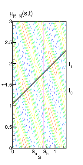
Figure 12: Instantaneous flux $\tilde{\mu}^{{\rm(a)}}_{{[5,-6]}}(s,t)$ along $C^{{\rm(a)}}$ for phase type (ii), corresponding to upstream propagation of the flux eddies as a counterpart of $\tilde{\mu}^{{\rm(a)}}_{{[5,6]}}(s,t)$ in Figure 6.

From a Lagrangian view point, integration (30) assumes spatial-temporal interaction by moving with a reference trajectory. The role of variability is determined by how the reference trajectory encounters flux eddies along $C$. From the view of the mean-eddy interaction by the variability, it is determined by how boxes and slices distribute diagonally in the domain of integration $(s_{a}:s_{b},t_{0}:t_{1})$. The rectangles surrounded by two vertical lines and two horizontal lines in the right bottom panel of Figure 6 (also left panel of Figure 12) exemplify a fixed domain of integration concerning definite TIME (Section 3.2). If we wish to compute TIME associated with a specific event of flow dynamics, a more geometrically complex domain can be judiciously chosen. For finite-time TIME, the domain increases as $t$ progresses.

To highlight the spatio-temporal interaction in (30), we introduce spatial and temporal integrations of $\tilde{\mu}^{C}_{i}(s,t)$ not associated with transport directly. Spatial integration at time $t$ is $\int_{s_{a}}^{s_{b}}\tilde{\mu}^{C}_{i}(s,t)ds=F^{C}_{i}f_{i}(t)$, where

$$F^{C}_{i}\equiv\sigma_{i}\int_{s_{a}}^{s_{b}}\mu^{C}_{i}(s)ds~{}:$$ (31)

is along a horizontal line and measures the spatial bias (Table 2). If it is nonzero, then net instantaneous flux oscillates with $f_{i}(t)$ and may lead to biased distribution of signed pseudo-lobes. In contrast, temporal integration is along a vertical line. Over the entire time interval $t\in[t_{-},t_{+}]$, it must be zero at any $s$, i.e., $\int_{t_{-}}^{t_{+}}\tilde{\mu}^{C}_{i}(s,t)dt=0$.

5 Graphical approach

Using the atmospheric model, we demonstrate the graphical approach for individual cases. Given $a^{C}_{\diamond}(s,t;s_{a}:s_{b},t_{0}:t_{1})$, spatial coherency and temporal evolution of transport is naturally described in terms of pseudo-PIPs and pseudo-lobes (Section 3). Some phenomena described below will be revisited in the next section using the analytic approach.

5.1 Finite-time TIME across the jet axis $C^{{\rm(a)}}$

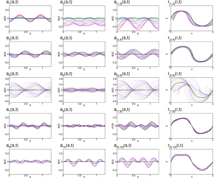
Figure 8: Envelopes of $a^{{\rm(a)}}_{2n-1}(s,t)$, $a^{{\rm(a)}}_{2n}(s,t)$ and $a^{{\rm(a)}}_{{[2n-1,2n]}}(s,t)$ in the $(s,a)$ space (panels in three left columns, respectively) and $r^{{\rm(a)}}_{{[2n-1,2n]}}(l,t)$ in the ${\bf{x}}$ space (panels in right column) along $C^{{\rm(a)}}$ where 20 envelopes are taken at every one half $T^{{\rm(a)}}$. The scales of $a^{{\rm(a)}}$ for $a^{{\rm(a)}}_{{5}}(s,t)$, $a^{{\rm(a)}}_{{6}}(s,t)$, and $a^{{\rm(a)}}_{{[5,6]}}(s,t)$ differ from others due to large amplitude, while $r^{{\rm(a)}}_{{[5,6]}}(s,t)$ is unscaled for comparison with pseudo-lobes of other pairs in ${\bf{x}}$.

We consider the finite-time TIME $a^{{\rm(a)}}_{\diamond}(s,t)=a^{{\rm(a)}}_{\diamond}(s,t;s^{\dagger}:s,t^{\dagger}:t)$ for $C^{{\rm(a)}}$, from time $t^{\dagger}$ up to the present $t$. We use the spatial periodic condition $\tilde{\mu}^{{\rm(a)}}_{\diamond}(s,t)=\tilde{\mu}^{{\rm(a)}}_{i}(s+T^{{\rm(a)}},t)$, where $T^{{\rm(a)}}=1.260549$ is the period of $C^{{\rm(a)}}$. As $t$ progresses, $a^{{\rm(a)}}_{\diamond}(s,t)$ changes because $\tilde{\mu}^{{\rm(a)}}_{\diamond}(s,t)$ keeps adding to the integration. Figure 8 shows the evolution of pseudo-lobes as 20 envelopes of $a^{{\rm(a)}}_{\diamond}(s,t)$ taken at every $T^{{\rm(a)}}/2$.

We start with the third pair $[5,6]$ whose pseudo-lobes have larger width and amplitude than any other pairs. Neither mode 5 nor 6 has spatial bias due to the symmetry (Figure 4). Mode 5 has a total of six flux eddies along $C^{{\rm(a)}}$. The two opposite-signed ones at $s=0.3157$ and $0.9454$ are much stronger than the others (Figure 5). As they pulsate, a diagonal line can go through the boxes associated with these two flux eddies when they have the same sign. By considering only them, the two opposite-signed pseudo-lobes emanate along $C^{{\rm(a)}}$ in $a^{{\rm(a)}}_{{5}}(s,t)$. It also leads to $\Gamma^{{\rm(a)}}_{{5}}\sim 1$: the most efficient spatio-temporal interaction as we shall see in the next section. In mode 6, the two pairs replace those two flux eddies in mode 5 (Figure 6). This process can be also thought as $\Gamma^{{\rm(a)}}_{{6}}\sim 1$; however, it is not as efficient as that for mode 5. Therefore, $a^{{\rm(a)}}_{{6}}(s,t)$ has two opposite-signed pseudo-lobes with smaller amplitude. Given the temporal phase condition (6) and the spatial phase type (i) of (28), modes 5 and 6 cooperate to form two large pseudo-lobes in $a^{{\rm(a)}}_{{[5,6]}}(s,t)$.

For any other pairs, one of the two modes has no spatial bias and almost satisfies the spatial regularity, i.e., $|F_{i}^{{\rm(a)}}|=0$ and $S^{{\rm(a)}}_{i}=T^{{\rm(a)}}/2N^{(\phi)}_{i}$ for $i=1,4,8$ and $9$ (Figure 6 for mode 1). The pseudo-lobes of these modes have a wave number $N^{(\phi)}_{i}$ pattern. Other modes have non-zero $|F_{i}^{{\rm(a)}}|$, mainly due to the same-signed flux eddies centered at $s=0.3157$ and $0.9454$. This $|F^{{\rm(a)}}_{i}|$ effect leads to a biased distribution of the signed pseudo-lobes. It is more substantial for even modes, embraced by the phase of $f_{i}(t)$ starting from $t^{\dagger}(=0)$ until $T^{({\bf{u}})}_{i}$ when the phase reverses. Accordingly, $a^{{\rm(a)}}_{{2}}(s,t)$ is heavily dominated by negative pseudo-lobes due to the spatial, temporal, and spatio-temporal reinforcers as follows: 1) $|F^{{\rm(a)}}_{{2}}|$ is large because the two negative flux eddies are much wider and stronger than the two positive ones; 2) the phases of $f_{{2}}(t)$ heighten the $|F^{{\rm(a)}}_{{2}}|$ effect; 3) the small characteristic ratio $\Gamma^{{\rm(a)}}_{{2}}\ll 1$ allows the $|F^{{\rm(a)}}_{{2}}|$ effect to spread over $C^{{\rm(a)}}$ along all diagonal lines (Figure 6 for mode 2). Biased pseudo-lobes are also observed in $a^{{\rm(a)}}_{{10}}(s,t)$, but not as significant as in $a^{{\rm(a)}}_{{2}}(s,t)$, because the spatial and spatio-temporal reinforcers are weaker for mode 10. Odd modes show little bias and have $N^{(\phi)}_{i}$ pairs of signed pseudo-lobes in $a^{{\rm(a)}}_{{i}}(s,t)$. As a pair, negative pseudo-lobes almost always dominate $a^{{\rm(a)}}_{{[1,2]}}(s,t)$. The pseudo-lobes in $a^{{\rm(a)}}_{{[3,4]}}(s,t)$, $a^{{\rm(a)}}_{{[7,8]}}(s,t)$ and $a^{{\rm(a)}}_{{[9,10]}}(s,t)$ have a slight bias in their wave number $N^{(\phi)}_{2n-1}$ pattern.

How can these results be interpreted as atmospheric transport phenomena? We recall that the $n$-th Rossby traveling wave $(k_{(n)},l_{(n)})$ generates flux eddies along the reference jet as it propagates (straight) eastward with phase speed $b^{({\bf{u}})}_{{[2n-1,2n]}}$ along $l_{(n)}$ lines. The flux eddies so generated intensify when passing the trough and ridge where the jet flows faster. The phase speed $b^{(\phi)}_{{[2n-1,2n]}}$ is slower than $b^{({\bf{u}})}_{{[2n-1,2n]}}$. All waves have positive characteristic ratios $\Gamma^{{\rm(a)}}_{2n-1}<1$. Therefore, a reference trajectory passes flux eddies from behind.

For the third Rossby traveling wave $(k_{({3})},l_{({3})})=(2,2)$, this process leads to synchronized bursts of opposite-signed flux eddies over the trough and ridge that change sign every $T^{({\bf{u}})}_{{5}}$. The time interval between consecutive bursts approximately equals the flight-time of a reference particle from the trough to ridge, i.e., $T^{({\bf{u}})}_{{5}}\sim T^{{\rm(a)}}/2$. Therefore, a particle can be almost always pushed in the same direction by every burst. Thus, the envelope of transport has large amplitude. The wave number 1 pattern mainly emanates opposite-signed bursts at the ridge and trough. This process can be thought of as resonance between the reference jet and the wave.

For the first Rossby traveling wave $(k_{({1})},l_{({1})})=(1,2)$, the bursts have the same sign in mode 2, leading to a strong southward spatial bias $F^{{\rm(a)}}_{{2}}$. The positive phase of $f_{{2}}(t)$ supports this effect starting from $t^{\dagger}=0$ up to $T^{({\bf{u}})}_{i}$ until the phase reverses. The temporal variability of this wave is slow enough that kinematic advection by the underlying reference flow can spread the spatial bias effect all along $C^{{\rm(a)}}$. Thus, this wave strongly favors southward finite-time transport starting at $t^{\dagger}=0$. If starting at $t^{\dagger}=T^{({\bf{u}})}_{{1}}$, then it favors northward. The envelopes of transport show a shadow of a wave number $N^{(\phi)}_{{1}}=2$ pattern.

The fifth Rossby traveling wave $(k_{({5})},l_{({5})})=(3,2)$ has a northward spatial bias $F^{{\rm(a)}}_{{10}}$. Its effect is not as distinguished as $F^{{\rm(a)}}_{{2}}$ because the bursts are weaker and the temporal variability is too fast to spread the spatial bias. Thus, the envelopes of transport almost always sustain a wave number $N^{(\phi)}_{{10}}=3$ pattern with slight northward bias.

The second and fourth Rossby traveling waves $(k_{({2})},l_{({2})})=(2,1)$ and $(k_{({4})},l_{({4})})=(2,3)$ have little bias in the distribution of signed pseudo-lobes, because $f_{i}(t)$ dissipates the spatial bias. The envelopes of transport have the wave number $N^{(\phi)}_{{3}}=2$ and $N^{(\phi)}_{{7}}=3$ patterns, respectively.

For all waves, the area of pseudo-lobes fluctuates as they propagate along $C^{{\rm(a)}}$. Surprisingly, the fluctuation frequency and propagation phase speed have no direct tie to the corresponding flux eddies or reference flow. Using an analytic approach, we explain these phenomena in Section 6.1.

5.2 Definite TIME across the separatrix $C^{{\rm(u)}}$

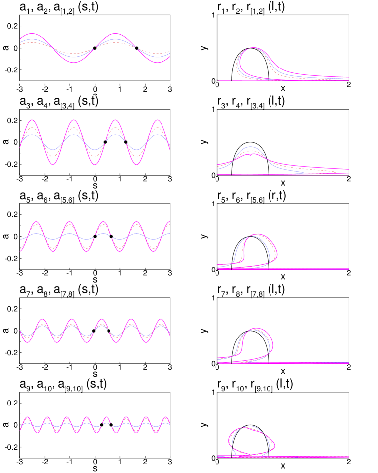
Figure 9: $a^{{\rm(u)}}_{2n-1}(s,t)$, $a^{{\rm(u)}}_{2n}(s,t)$ and $a^{{\rm(u)}}_{{[2n-1,2n]}}(s,t)$ in the $(s,a)$ space (left panels) and $r^{{\rm(u)}}_{2n-1}(l,t)$, $r^{{\rm(u)}}_{2n}(l,t)$ and $r^{{\rm(u)}}_{{[2n-1,2n]}}(l,t)$ in the ${\bf{x}}$ space (right panels) along $C^{{\rm(u)}}$ at $t^{*}=5$; solid and dashed lines are for even and odd modes, respectively, and thick line is for the pair. The circles are the upstream pseudo-PIP at $s^{*}$ downstream pseudo-PIP at $s^{*}+T^{({\bf{u}})}_{{2n-1}}$ for the positive pseudo-lobe ${\cal L}^{*}$. The pseudo-PIPs correspond to the diagonal lines in Figure 10.

We consider definite TIME $a^{{\rm(u)}}_{\diamond}(s,t)=a^{{\rm(u)}}_{\diamond}(s,t;-\infty:\infty,-\infty:\infty)$ across $C^{{\rm(u)}}$. We refer to the two segments of $C^{{\rm(u)}}$ as the “western” ($s<0$) and “eastern” ($s>0$) regions with respect to the trough ($s=0$). Due to the particular choice for the domain of integration along the separatrix, pseudo-lobes of $a^{{\rm(u)}}_{\diamond}(s,t)$ relate to lobes of Lagrangian transport theory up to the leading order (this is explained in Ide & Wiggins (2014b)). Because $C^{{\rm(u)}}$ is away from the flux alignment curve, any mode has an irregular distribution of flux eddies (Figure 5). Nonetheless, $a^{{\rm(u)}}_{\diamond}(s,t)$ shows some remarkable similarities. The pseudo-PIP sequence has a constant separation distance $T^{({\bf{u}})}_{i}$ in a unit of flight time. The pseudo-lobe sequence spreads homogeneously along $C^{{\rm(u)}}$. Because the sequence propagates with the reference flow without deformation in the $(s,a)$ space, it suffices to consider one snap shot of $a^{{\rm(u)}}_{\diamond}(s,t)$ (Figure 9). These are general properties of definite TIME and will be explained in Section 6.2. Due to the (anti-)symmetry in $\mu^{{\rm(u)}}_{i}(s)$ and $f_{i}(t)$, any $a^{{\rm(u)}}_{\diamond}(s,t)$ share the same pseudo-PIP sequence.

For example, mode 5 has two flux eddies in $\mu^{{\rm(u)}}_{{5}}(s)$ over both the western and eastern regions (Figure 5). The second and third flux eddies around the trough are positive. They are stronger than the first and fourth ones that are negative. The characteristic ratio over the positive ones are slightly larger than 0.5 in $\tilde{\mu}^{{\rm(u)}}_{{5}}(s,t)$ (Figure 7). Hence, a diagonal line can go through just about all boxes of spatio-temporal coherency while they have the same sign. For a given $\mu^{{\rm(u)}}_{{5}}(s)$, $f_{{5}}(t)$ has an effective $T^{({\bf{u}})}_{{5}}$ that enhances spatio-temporal interaction in $\tilde{\mu}^{{\rm(u)}}_{{5}}(s,t)$: all flux eddies may favor inflating the pseudo-lobes of $a^{{\rm(u)}}_{{5}}(s,t)$. In contrast, four flux eddies of the complementary mode 6 alternate the signs in $\mu^{{\rm(u)}}_{{6}}(s)$ and have relatively small characteristic ratios in $\tilde{\mu}^{{\rm(u)}}_{{6}}(s,t)$. Contributions from these pulsating flux eddies tend to hinder each other along the diagonal line, resulting in the flat pseudo-lobes of $a^{{\rm(u)}}_{{6}}(s,t)$. Mode 5 rules $a^{{\rm(u)}}_{{[5,6]}}(s,t)$ when the two modes are combined (Figure 9).

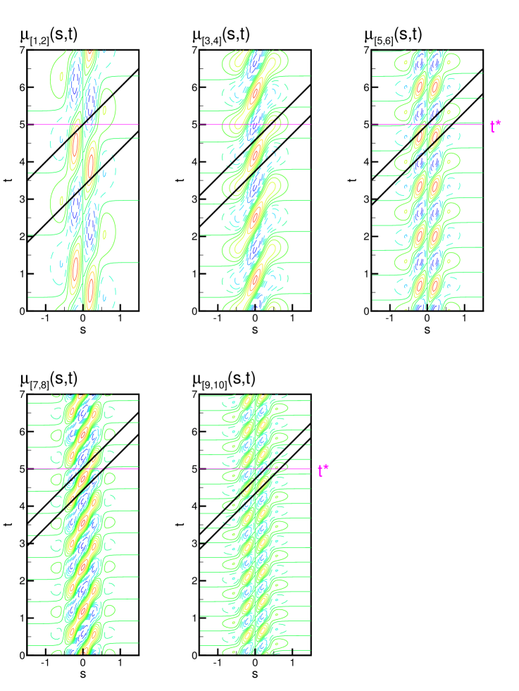
Figure 10: Instantaneous flux $\tilde{\mu}^{{\rm(u)}}_{{[2n-1,2n]}}(s,t)$ for the five Rossby traveling waves along $C^{{\rm(u)}}$. The two diagonal lines correspond to the two pseudo-PIPs of the pseudo-lobe ${\cal L}^{*}$, as indicated by the circles in Figure 9; $t^{*}$ is the evaluation time.

For the $n$-th Rossby traveling wave as a pair $[2n-1,2n]$, downstream propagation of flux eddies in $\tilde{\mu}^{{\rm(u)}}_{{[2n-1,2n]}}(s,t)$ can be irregular and discontinuous (Figure 10). For the first, third, and fifth Rossby traveling waves, propagation splits into the two segments because the flux eddy along the alignment curve does not reach $C^{{\rm(u)}}$ at the trough ($x=1/2$) in $\phi_{{2}}({\bf{x}})$, $\phi_{{7}}({\bf{x}})$ and $\phi_{{10}}({\bf{x}})$, respectively. This leads to the propagation that looks as if the flux eddies disappear at the trough ($s=0$) and reappear in the downstream with a reversed sign. For the second Rossby traveling wave, propagation in $\tilde{\mu}^{{\rm(u)}}_{{[3,4]}}(s,t)$ is irregular but continuous because all flux eddies in $\phi_{{3({\bf{x}})}}$ and $\phi_{{4}}({\bf{x}})$ reach $C^{{\rm(u)}}$ for $0<x<1$. The fourth Rossby traveling wave also has a continuous propagation in $\tilde{\mu}^{{\rm(u)}}_{{[7,8]}}(s,t)$, although $C^{{\rm(u)}}$ skips a couple of flux eddies in $\phi_{{7}}({\bf{x}})$ and $\phi_{{8}}({\bf{x}})$ along the flux alignment curve. For these second and fourth Rossby traveling waves, propagating flux eddies in $\tilde{\mu}^{{\rm(u)}}_{{[2n-1,2n]}}(s,t)$ intensify when passing the trough.

Using the graphical approach, we examine the role of Rossby traveling waves in transport with a focus on a pseudo-lobe. We show what the positive pseudo-lobe ${\cal L}^{*}={\cal L}^{({\bf{u}})}_{{[2n-1,2n],0:1}}(t^{*})$ closest to the trough along $C^{{\rm(u)}}$ at time $t^{*}=5$ is made of. The two pseudo-PIPs that define ${\cal L}^{*}$ are shown in Figure 9 by the circles. We denote the upstream pseudo-PIP by $s^{({\bf{u}})}_{{[2n-1,2n],0}}(t^{*})=s^{*}$. Then the downstream one is $s^{({\bf{u}})}_{{[2n-1,2n],1}}(t^{*})=s^{*}+T^{({\bf{u}})}_{{2n-1}}$.

The two diagonal lines in Figure 10 go through the two pseudo-PIPs. Because the definite TIME $a^{({\bf{u}})}_{{[2n-1,2n]}}(s,t)$ propagates with the reference flow, they also coincide with the trajectories of the two pseudo-PIPs. The region bounded by these diagonal lines shows the makeup of ${\cal L}^{*}$. The propagation phase speed of flux eddies is slower than a reference trajectory for any wave, i.e., $\Gamma^{{\rm(u)}}_{{2n-1}}<1$.

For the first, third, and fifth Rossby traveling waves, the region contains four propagating flux eddies. Over the western region, a positive follows a negative. The order reverses over the eastern region. The maximum amplitude of ${\cal L}^{*}$ occurs at $s^{*}+T^{({\bf{u}})}_{{2n-1}}/2$. The corresponding reference trajectory moves through the positive flux eddies over the western region, reaches the trough at the same time as the head of the same flux eddy, and moves into another positive flux eddy over the eastern region. Therefore, $a^{{\rm(u)}}(s^{*}+T^{({\bf{u}})}_{{2n-1}}/2,t^{*})$ has equal and positive contributions from both regions. Such spatio-temporal interaction can be more efficient for smaller $\Gamma^{{\rm(u)}}_{{2n-1}}$ if $\Gamma^{{\rm(u)}}_{{2n-1}}<1$. Therefore, the first Rossby traveling wave is most efficient among the three due to the large ${\bar{T}}^{({\bf{u}})}_{{1}}$. At $\Gamma^{{\rm(u)}}_{{2n-1}}\approx 1$, contribution from either region becomes zero. (compare $\mu^{{\rm(u)}}_{{[1,2]}}(s,t)$ and $\mu^{{\rm(u)}}_{{[9.10]}}(s,t)$ in Figure 10).

In the upstream portion of ${\cal L}^{*}$, a negative contribution develops from the trough due to the second propagating flux eddy over the eastern region and it propagates upstream. At the upstream pseudo-PIP $s^{*}$, this negative contribution balances the positive contribution from the western region. Conversely, in the downstream portion of ${\cal L}^{*}$, negative contribution develop from the trough over the western region and propagate downstream. At the downstream pseudo-PIP $s^{*}+T^{({\bf{u}})}_{{2n-1}}$, it balances the positive contribution from the eastern region.

By tracing its dynamic roots in $\tilde{\psi}_{{[2n-1,2n]}}({\bf{x}},t)$, we find that the reference trajectory $(s^{*}+T^{({\bf{u}})}_{{2n-1}}/2-t^{*}+\tau,\tau)$ for the maximum pseudo-lobe amplitude goes through the trough at the same time as the center of a positive dynamic eddy in the south reaches the trough over the recirculating cell. In addition, $(s^{*}+T^{({\bf{u}})}_{{2n-1}}-t^{*}+\tau,\tau)$ for the downstream pseudo-PIP and the head of that dynamic eddy arrive at the trough simultaneously; $(s^{*}-t^{*}+\tau,\tau)$ for the upstream pseudo-PIP and the tail of the dynamic eddy go through the trough simultaneously.

Accordingly, the pseudo-lobe sequence of these Rossby traveling waves appears to evolve as if they move with the dynamic eddies in ${\bf{x}}$. Note that the pseudo-lobe sequence itself propagates with the reference flow along $C^{{\rm(u)}}$.

The role of variability completely differs for the second and fourth Rossby traveling waves. The two diagonal lines associated with ${\cal L}^{*}$ mainly contain a positive propagating flux eddy. Due to $\Gamma^{{\rm(u)}}_{{2n-1}}<1$, the western region includes a negative propagating flux eddy that succeeds the positive. Over the eastern region, a negative one precedes.

The center of the main positive flux eddy and the reference trajectory $(s^{*}+T^{({\bf{u}})}_{{2n-1}}/2-t^{*}+\tau,\tau)$ going through the center of ${\cal L}^{*}$ reaches the trough simultaneously. Therefore the trajectory receives the maximum contribution from it.

Clearly, the maximum amplitude of ${\cal L}^{*}$ occurs along the reference trajectory that goes though the trough at the same time as the center of the positive flux eddy does. In the upstream portion of ${\cal L}^{*}$, a negative contribution develops from the upstream of $C^{{\rm(u)}}$ due to the succeeding negative flux eddy over the western region. In contrast, the downstream portion of ${\cal L}^{*}$ develops a negative contribution from the downstream of $C^{{\rm(u)}}$ due to the preceding negative flux eddy over the eastern regions.

Such spatio-temporal interaction along the diagonal line is most efficient at $\Gamma^{({\bf{u}})}_{{2n-1}}\approx 1$, unlike the three Rossby traveling waves mentioned above. Moreover, we find that the spatio-temporal interaction for the fourth Rossby traveling wave is inefficient, because intensifications of the positive flux eddy off the trough (around $|s|\approx 0.3$) are wasted along the two diagonal lines for the pseudo-PIPs. If $T^{({\bf{u}})}_{{7}}$ decreases to increase $\Gamma^{{\rm(u)}}_{{7}}$ to near 1, then these intensifications can significantly help enhance $a^{{\rm(u)}}(s,t^{*})$ around $s\sim s^{*}+T^{({\bf{u}})}_{{2n-1}}/2$.

By tracing the dynamic root of the spatio-temporal interaction for the second Rossby traveling wave, we find that the center of a positive dynamic eddy in $\tilde{\psi}_{{[3,4]}}({\bf{x}},t)$ and the reference trajectory associated downstream pseudo-PIP go though the trough simultaneously. After $T^{({\bf{u}})}_{{3}}$, the center of the succeeding positive dynamic eddy and the reference trajectory of the upstream pseudo-PIP go though the trough together. Accordingly, the evolution of the pseudo-lobe sequence appears to succeed the dynamic eddies with a $T^{({\bf{u}})}_{{3}}/2$ time-lag.

For the fourth Rossby traveling wave, two southern dynamic eddies in each column act together. The evolution of the pseudo-lobe sequence succeeds the dynamic eddies in the middle row with a $T^{({\bf{u}})}_{{7}}/2$ time-lag.

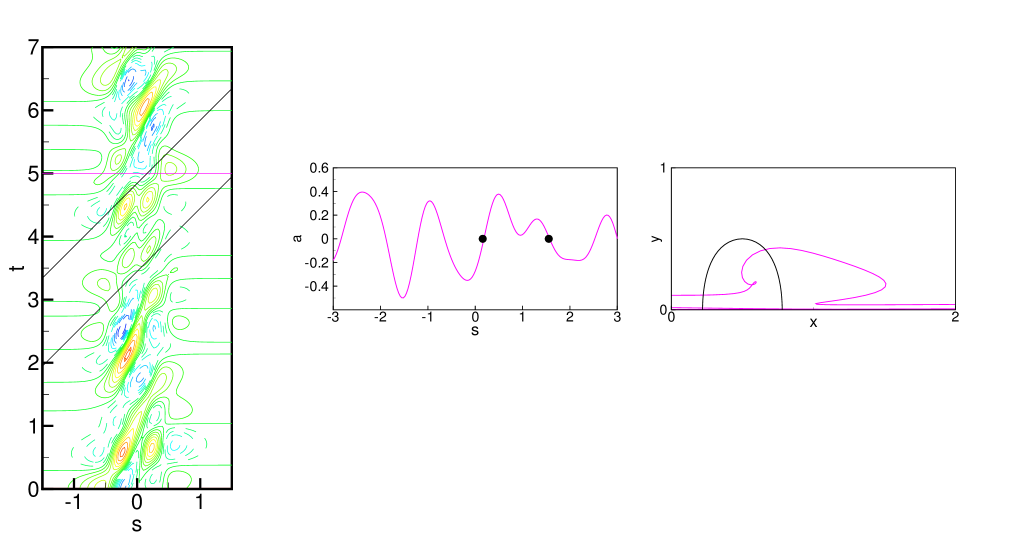
Figure 11: Same as Figures 9 and 10, but for all five Rossby waves together.

Definite TIME due to all five Rossby traveling waves is shown in Figure 11. The graphical approach can be used in two ways. Given $a^{({\bf{u}})}(s,t)$, comparing $\tilde{\mu}_{{[2n-1,n]}}^{({\bf{u}})}(s,t)$ to $\tilde{\mu}^{({\bf{u}})}(s,t)$ identify the variability which is responsible for individual pseudo-lobes. Inversely, given individual $\tilde{\mu}_{{[2n-1,n]}}^{({\bf{u}})}(s,t)$, we obtain how they collaborate to produce net $a^{({\bf{u}})}(s,t)$. Finally, we note that the graphical approach can be used to identify role of variability when $f_{2n-1}(t)$ is irregular, i.e., $T^{({\bf{u}})}_{2n-1}$ varies in time.

6 Analytical approach

Motivated by Section 5, we now explore the underlying properties of finite-time and definite TIME that are relevant to large-scale geophysical flows. We highlight the results of the analytical approach in this section while details are provided in Appendix A.

6.1 Finite-time TIME

To identify the basic properties of finite-time transport $a^{C}_{\diamond}(s,t)=a^{C}_{\diamond}(s,t:s-t+t^{\dagger}:s,t-t^{\dagger}:t)$, we consider an idealized case: $\tilde{\mu}^{C}_{\diamond}(s,t)$ arising from regularly distributed flux eddies (see upper panels of Figure 6). If $C$ is periodic with period $T^{C}$ and $\mu^{C}_{i}(s)$ has $2N^{(\phi)}_{i}$ flux eddies like $C^{{\rm(a)}}$, then $S^{C}_{i}=T^{C}/2N^{(\phi)}_{i}$ gives $\Gamma^{C}_{i}=T^{C}/(2N^{(\phi)}_{i}T^{({\bf{u}})}_{i})$. First, we revisit the graphical approach $a^{C}_{\diamond}(s,t)$. This time, we focus on a single diagonal line of integration where the evaluation point $s=s^{\dagger}-t^{\dagger}+t$ moves downstream as $t$ increases.

• Mode $i$: The corresponding $\tilde{\mu}^{C}_{i}(s,t)$ has uniform boxes of a size $S^{C}_{i}\times T^{({\bf{u}})}_{i}$ (Figure 6). Integration (30a) may be most efficient for $\Gamma^{C}_{i}\approx 1$, because $a^{C}_{i}(s,t)$ can increase monotonically if the diagonal line of integration goes through one box to another without ever changing the sign of $\tilde{\mu}^{C}_{i}(s^{\dagger}-t^{\dagger}+t,t)$ as $t$ increases. In contrast, for $\Gamma^{C}_{i}\not\approx 1$, $a^{C}_{i}(s,t)$ fluctuates because $\tilde{\mu}^{C}_{i}(s^{\dagger}-t^{\dagger}+t,t)$ changes sign regularly by running through one box to another. For $\Gamma^{C}_{i}\gg 1$, $a^{C}_{i}(s,t)$ oscillates with a period roughly $2T^{({\bf{u}})}_{i}$ because the diagonal line goes through horizontally-thin boxes in the $(s,t)$ space. In contrast, for $\Gamma^{C}_{i}\ll 1$, $a^{C}_{i}(s,t)$ oscillates with a period roughly $2S^{C}_{i}$.

• Pair $[i,i+1]$: The corresponding $\tilde{\mu}^{C}_{[i,i+1]}(s,t)$ has slanting contours in the $(s,t)$ as shown in right bottom panel of Figure 6 for phase type (i) and left panel of Figure 12 for (ii). It is clear that $a^{C}_{[i,i+1]}(s,t)$ for phase type (ii) oscillates faster because $\tilde{\mu}^{C}_{[i,i+1]}(s,t)$ changes sign more frequently along the diagonal line.

Next, we use the analytical approach on the idealized models to quantify the spatio-temporal interaction as a function of $\Gamma^{C}_{i}$ (Appendix A.1, Model case 1.1). Highlights of the phenomena follow.

• Mode $i$: Finite-time TIME can be represented as a sum of low- and high-frequency responses to pulsating flux eddies whose amplitude and period depend on $S^{C}_{i}/(1-\Gamma^{C}_{i})$ and $S^{C}_{i}/(1+\Gamma^{C}_{i})$, respectively (A.2). Based on amplitude, the low-frequency tends to overcome the high-frequency response; especially for $\Gamma^{C}_{i}\approx 1$. At $\Gamma^{C}_{i}=1$, the low-frequency response becomes resonant and exhibits linear growth as in (A.2d). Table 2 summarizes the predicted values of the amplitude and period along $C^{{\rm(a)}}$.

• Pair $[i,i+1]$: The response is restricted to low-frequency for phase type (i) and high-frequency for phase type (ii), confirming the results using the graphical approach.

We see from Table 1 that $\Gamma^{C}_{i}$ is fairly small with respect to 1 for any Rossby traveling wave. This means that, if the wave travels faster, then more TIME can be expected. If we use $N^{(\phi)}_{{3}}=1$ (Section 5) for pair $[3,4]$, then $\Gamma^{C}_{{3}}\approx 1$ (Table 2) leads to a large values of $S^{C}_{i}/(1-\Gamma^{C}_{i})$. This would explain the extremely large pseudo-lobes when compared to other pairs.

Using the spatial phase conditions (25) and (28),

$$a^{C}_{\diamond}(s,t)\approx-a^{C}_{\diamond}(s-S^{C}_{i},t)~{}$$ (32)

holds independent of the temporal components $f_{i}(t)$ and $f_{i+1}(t)$. This confirms the observations made in Section 5 that $a^{C}_{\diamond}(s,t)$ along $C^{{\rm(a)}}$ may have the same wave number as the flux eddies for $|F^{C}_{i}|\neq 0$ is nonzero. Therefore, the separation distance of the pseudo-PIP sequence is a constant $\triangle s^{C}_{{\diamond,j:j+1}}=S^{C}_{i}$. At time $t$, the corresponding pseudo-lobe sequence has a homogeneous configuration with alternating sign along $C$.

The analytical approach in Appendix A.1 (Model case 1.2) relates the geometry and evolution of pseudo-lobes to the characteristic ratio $\Gamma^{C}_{i}$. For simplicity, we summarize the two cases of response for $a^{C}_{[i,i+1]}(s,t)$. The case for $a^{C}_{i}(s,t)$ is given as a linear sum of the two responses.

• A low-frequency response for phase type (i) (A.9): A pseudo-lobe sequence propagates downstream at a constant phase speed $(1+\Gamma^{C}_{i})/2$ (A.9a), which averages the phase speed of a reference trajectory and flux eddy propagation. At $\Gamma^{C}_{i}=1$ when the flux eddies propagate with the reference flow, so too do all pseudo-lobes whose signed area $A^{C}_{{[i,i+1],j:j+1}}(t)$ grows linearly in $t$ (A.9d). For $\Gamma^{C}_{i}\neq 1$, maximum amplitude of $A^{C}_{{[i,i+1],j:j+1}}(t)$ oscillates with the period $4S^{C}_{i}/(1-\Gamma^{C}_{i})$. As $\Gamma^{C}_{i}$ varies from 1, $A^{C}_{{[i,i+1],j:j+1}}(t)$ decays like $1/\Gamma^{C}_{i}$.

• A high-frequency response for phase type (ii) (A.10): The same formulae obtained for the low-frequency response hold by replacing $\Gamma^{C}_{i}$ with $-\Gamma^{C}_{i}$. The main difference appears in propagation where all pseudo-lobes travel downstream for $\Gamma^{C}_{i}<1$ and upstream for $\Gamma^{C}_{i}>1$. At $\Gamma^{C}_{i}=1$, $a^{C}_{{[i,i+1]}}(s,t)$ behaves like standing waves with oscillation period $2T^{({\bf{u}})}_{i}$.

Table 2 shows the predicted phase speed of the pseudo-lobes for our example problem.

6.2 Definite TIME

Here we explore general properties associated with definite TIME $a^{C}_{\diamond}(s,t)=a^{C}_{\diamond}(s,t;s_{a}:s_{b},t_{0}:t_{1})$ for a fixed $(s_{a}:s_{b},t_{0}:t_{1})$, where $C$ is not necessarily a separatrix. Substituting temporal phase conditions (4) and (6) into (30b) gives two useful relations:

$$a^{C}_{\diamond}(s,t) \approx -a^{C}_{\diamond}(s-T^{({\bf{u}})}_{i},t)~{},$$ (33a)

$$a^{C}_{\diamond}(s,t) \approx a^{C}_{\diamond}(s+\triangle t,t+\triangle t)~{}.$$ (33b)

The first relation means that the separation distance $\triangle s^{C}_{{\diamond,j:j+1}}$ of the pseudo-PIP sequence is a constant $T^{({\bf{u}})}_{i}$ and the pseudo-lobe sequence has a homogeneous configuration with alternating signs in the $(s,a)$ space. This result can be confirmed graphically along the two diagonal lines of integration separated by $T^{({\bf{u}})}_{i}$ in $t$ (Figure 7). The second relation means that the pseudo-PIP and pseudo-lobe sequences propagate with the reference flow without deformation in the $(s,a)$ space. This invariance can be confirmed graphically along any diagonal line.

Motivated by Section 5.2 using the graphical approach, we consider the following two cases. The first case focuses on contributions from individual flux eddies in $\mu^{C}_{i}(s)$. This is useful to understand not only the role of individual flux eddies but also how they are combined in the total transport. The second case considers the spectral response of the spatial component $\mu^{C}_{i}(s)$ to the temporal PC $f_{i}(t)$. This helps us understand the effect of having more than one spectral component in $f_{i}(t)$ or sensitivity with respect to temporal frequency. Details of both analyses are given in Appendix A.2 for both cases.

We first consider the contribution of $a^{C}_{{\diamond.p}}(s,t)$ from the $p$-th flux eddy, where the subscript $\{\cdot\}_{{\diamond.p}}$ corresponds to the $p$-th flux eddy of variability $\diamond$. The relations in (33) hold for $a^{C}_{{\diamond.p}}(s,t)$ by adjusting $(s_{a}:s_{b},t_{0}:t_{1})$ to a corresponding vertical column in $\tilde{\mu}^{C}_{\diamond}(s,t)$ (A.14). The analytical approach based on a highly idealized model in Appendix A.2 (Model case 2.1) illuminates the dependence on $\Gamma^{C}_{i.p}$, as briefly summarized below.

• Mode $i$: Definite TIME $a^{C}_{i.p}(s,t)$ splits into two elements: amplitude and normalized configuration (A.16a). The normalized configuration is based on $f_{i}(s-t)$, confirming the constant separation distance $T^{({\bf{u}})}_{i}$ of the pseudo-PIP sequence. The amplitude $M^{C}_{i.p}$ has a maximum at $\Gamma^{C}_{i.p}=1$ and decays like $S^{C}_{i}/\{1-(\Gamma^{C}_{i.p})^{2}\}$ with fluctuations (A.16d). Since the fluctuation is due to cancelation along the diagonal line by frequent sign changes of $f_{i}(t)$, for an even integer $\Gamma^{C}_{i}$, the spatio-temporal interaction is subharmonic and cancels the net transport completely.

• Pair $[i,i+1]$: For the complementary mode of the pair, $a^{C}_{i+1.p}(s,t)$ also splits into the two elements. The normalized configuration is based on $f_{i}(s-t)$, but there is a phase shift $\pm 2\theta^{C}_{[i,i+1].p}$ from $a^{C}_{i.p}(s,t)$ where $+$ and $-$ for phase type (i) and (ii) of (28), respectively. As a pair, amplitude $M^{C}_{{[i,i+1].p}}$ has a fluctuating multiplication factor to $M^{C}_{i.p}$, while the normalized configuration has a phase shift $\pm\theta^{C}_{[i,i+1].p}$ from $a^{C}_{[i,i+1].p}(s,t)$ At $\Gamma^{C}_{i.p}=1$, phase type (i) has the maximum enhancement $a^{C}_{{[i,i+1].p}}(s,t)=2a^{C}_{i.p}(s,t)$ while phase type (ii) results in a complete suppression $a^{C}_{{[i,i+1].p}}(s,t)=0$. Therefore, $\Gamma^{C}_{i.p}$ governs how the two modes may incorporate each other in forming $a^{C}_{{[i,i+1].p}}(s,t)$.

Given contributions from individual flux eddies, the total $a^{C}_{\diamond}(s,t)$ can be given as a linear sum of individual contributions (Appendix A.2, Model case 2.2a).

The second is more general. It considers the total $a^{C}_{\diamond}(s,t)$ as a spectral response of the flux spatial component $\mu^{C}_{\diamond}(s)$ to the temporal variability $f(t)=\cos\pi t/T$ where $T$ is the characteristic time scale (Appendix A.2, Model case 2.2b). It is easy to show that $a^{C}_{\diamond}(s,t)$ consists of an amplitude $M^{C}_{i}$ and normalized configuration $f(s-t+\theta)$ where $\theta-t$ is the phase lag between the temporal forcing and geometry at a fixed $t$. Since $\mu^{C}_{i}(s)$ is given without specifying $S^{C}_{i}$, the efficiency of the spatio-temporal interaction is given as a function of $1/T$, rather than $\Gamma^{C}_{i}=S^{C}_{i}/T^{({\bf{u}})}_{i}$ (A.24b). By definition, the limit of the amplitude corresponds to the spatial bias: $\lim_{1/T\to 0}M^{C}_{i}=F^{C}_{i}$ (31).

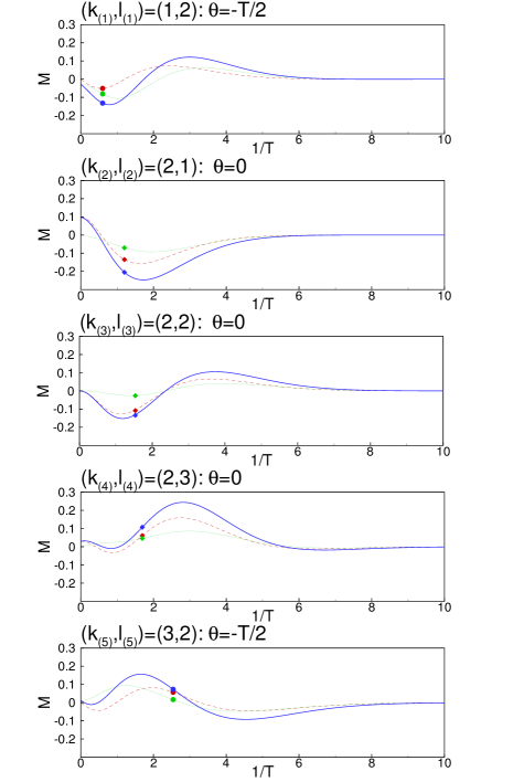
Figure 13: $M^{{\rm(u)}}_{\diamond}$ as function of $1/T$ using the spatial components $\mu^{{\rm(u)}}_{2n-1}(s)$ and $\mu^{{\rm(u)}}_{2n}(s)$ along $C^{{\rm(u)}}$ but $f(t)=\cos\pi t/T$ instead of $f_{2n-1}(t)$ and $f_{2n}(t)$, respectively. The symbols corresponding to $T=T^{({\bf{u}})}_{i}$ for the atmospheric model.

Figure 13 shows $M^{C}_{i}$ as a function of $1/T$ for the atmospheric model along $C^{{\rm(u)}}$. It also gives the sensitivity of definite transport with respect to the temporal component, given the spatial component of dynamic variability. We confirm our observation in Section 5.2 that the spatio-temporal interaction of the third Rossby traveling wave is efficient and that it is not for the forth and fifth Rossby traveling waves. We also confirms that the forth Rossby traveling wave can be enhanced significantly by decreasing $T$. The first and second Rossby traveling waves are also found to be efficient from the figure.

7 Concluding remarks

By combining a spatio-temporal analysis for variability and the geometrical method for transport, we have studied how variability affects transport of fluid particles and flow properties across a stationary boundary curve defined kinematically by a streamline of the mean flow. The Transport Induced by Mean-Eddy Interaction (TIME) theory is natural for this because it presents transport as the integration of the spatio-temporal interaction between the steady reference flow and the unsteady anomaly. Through the spatially nonlinear interaction with the reference flow, the dynamic mode $i$ in the velocity anomaly leads to the flux mode $i$. Therefore, global evolution of dynamic eddies and flux eddies in the flow field can be spatially different. Along the boundary curve $C$ across which we evaluate transport, the characteristic length-scale $S^{C}_{i}$ is determined by the flux eddies in a unit of flight-time, while the characteristic time-scale $T^{({\bf{u}})}_{i}$ is given by the corresponding dynamic mode. The non-dimensional characteristic ratio $\Gamma^{C}_{i}=S^{C}_{i}/T^{({\bf{u}})}_{i}$ rates as the most important parameter by providing the spatio-temporal coherency of instantaneous flux. At $\Gamma^{C}_{i}=1$, the flux variability and the reference flow dynamics are resonant. When modes $i$ and $i+1$ are a dynamically coherent pair, $\Gamma^{C}_{i}$ may correspond to the propagation speed of flux eddies along $C$.

We have presented a graphical approach for individual cases and an analytical approach for general properties of transport. We focused on the two types of transport that may be most relevant to large-scale geophysical flows. One concerns finite-time transport starting from an initial time up to the present time. For each mode, the transport consists of low- and high-frequency responses to the pulsating flux eddies. The low-frequency response relates to downstream propagation of flux eddies and high-frequency response to upstream. The pseudo-lobes of both responses have the same width $S^{C}_{i}$ as the flux eddies. The propagation phase speed averages the reference flow and flux eddies, i.e., envelopes of transport is associated neither with particle motion nor dynamics (or even flux) waves. The amplitude and oscillation period of pseudo-lobes depend on $S^{C}_{i}/(1-\Gamma^{C}_{i})$ for low-frequency response and $S^{C}_{i}/(1+\Gamma^{C}_{i})$ for high-frequency response, respectively. Hence, the low-frequency response tends to dominate the high.

The other type concerns definite transport. The corresponding pseudo-lobes propagate with the reference flow without changing area. The width of the pseudo-lobes is determined by the characteristic time-scale $T^{({\bf{u}})}_{i}$ as flight-time along $C$ and has nothing to do with flux eddy structure. The amplitude decays like $S^{C}_{i}/\{1-(\Gamma^{C}_{i})^{2}\}$ with fluctuation as $\Gamma^{C}_{i}$ increases. Moreover, the pseudo-lobes appear to move with the dynamic eddies with a possible phase-lag, although it propagates downstream with the reference flow.

In the case where $C$ is a separatrix, the spatial segment and temporal interval can be chosen to be bi-infinite. Such a definite transport is equivalent to the Melnikov function for Lagrangian lobe dynamics (as shown in Ide & Wiggins (2014b)). Therefore, it can shed some light on the role of variability for Lagrangian particle transport as well.

By applying the graphical and analytical approaches to the kinematic model of the large-scale atmospheric flow for a blocked flow, we have examined the role of Rossby traveling waves in transport. We have identified similarities and differences in their spatio-temporal interaction.

Because of its flexibility, the framework presented here can be modified and extended for various types of transport studies.

Appendix A idealized model for TIME

A.1 Category 1: Finite-time TIME

Model case 1.1: Efficiency

We explore the dependence on characteristic scales using a highly idealized model that satisfies the spatial and temporal phase condition given by (4), (6), (25) and (28).

1. Single mode $i$: We consider a model:

   $$\tilde{\mu}^{C}_{i}(s,t) = \sigma^{C}_{i}\cos\left(\frac{\pi}{S^{C}_{i}}s\right)\cos\left(\frac{\pi}{T^{({\bf{u}})}_{i}}t\right)~{},$$ (A.1)

   where $\sigma^{C}_{i}$ has a unit of (velocity)² corresponding to $\sigma_{i}|{\bar{{\bf{u}}}}({\bar{\bf{x}}}^{C}(s))||{\bf{u}}_{i}({\bar{\bf{x}}}^{C}(s))|$ as in (24b). A straightforward integration of (30a) using (A.1) gives an analytical form for $a^{C}_{i}(s,t)=a^{C}_{i}(s,t;s^{\dagger}:s,t^{\dagger}:t)$:

   $$a^{C}_{i}(s,t) = b^{C}_{i}(t;s^{\dagger},t^{\dagger})+d^{C}_{i}(t;s^{\dagger},t^{\dagger})-[b^{C}_{i}(t^{\dagger};s^{\dagger},t^{\dagger})+d^{C}_{i}(t^{\dagger};s^{\dagger},t^{\dagger})]~{},$$ (A.2a)

   where $$s^{\dagger}=s-t+t^{\dagger}$$, and

   $$b^{C}_{i}(t;s^{\dagger},t^{\dagger}) = \sigma^{C}_{i}\left\{\begin{array}[]{ll}t~{}\cos\{\frac{\pi}{S^{C}_{i}}(s^{\dagger}-t^{\dagger})\}~{},&\mbox{for $\Gamma^{C}_{i}=1$}~{},\\ \frac{S^{C}_{i}}{2\pi(1-\Gamma^{C}_{i})}~{}\sin\{\frac{\pi}{S^{C}_{i}}\left(1-\Gamma^{C}_{i}\right)t+\frac{\pi}{S^{C}_{i}}(s^{\dagger}-t^{\dagger})\}~{},&\mbox{for $\Gamma^{C}_{i}\neq 1$}~{}:\end{array}\right.$$ (A.2d)

   $$d^{C}_{i}(t;s^{\dagger},t^{\dagger}) = \begin{array}[]{l}\sigma^{C}_{i}\frac{S^{C}_{i}}{2\pi(1+\Gamma^{C}_{i})}~{}\sin\{\frac{\pi}{S^{C}_{i}}\left(1+\Gamma^{C}_{i}\right)t+\frac{\pi}{S^{C}_{i}}(s^{\dagger}-t^{\dagger})\}~{},\end{array}$$ (A.2f)

   are respectively the low- and high-frequency responses of TIME to mode $i$. The last two terms of the right-hand side in (A.2a) are initial condition to satisfy $a^{C}(s,t^{\dagger})=0$.

2. A dynamically coherent pair $[i,i+1]$: Using $S^{C}_{i}=S^{C}_{i+1}$, instantaneous flux can be written in a form:

   $$\tilde{\mu}^{C}_{[i,i+1]}(s,t) = \left\{\begin{array}[]{rl}\sigma^{C}_{i}\cos\left\{\frac{\pi}{S^{C}_{i}}\left(s-\Gamma^{C}_{i}t\right)\right\}~{},&\mbox{for phase type (i)}~{},\\ \sigma^{C}_{i}\cos\left\{\frac{\pi}{S^{C}_{i}}\left(s+\Gamma^{C}_{i}t\right)\right\}~{},&\mbox{for phase type (ii)}~{}.\end{array}\right.$$ (A.5)

   The corresponding TIME function is:

   $$a^{C}_{[i,i+1]}(s,t) = \left\{\begin{array}[]{rl}2b^{C}_{i}(t;s^{\dagger},t^{\dagger})~{}-2b^{C}_{i}(t^{\dagger};s^{\dagger},t^{\dagger})~{},&\mbox{for phase type (i)}~{},\\ 2d^{C}_{i}(t;s^{\dagger},t^{\dagger})~{}-2d^{C}_{i}(t^{\dagger};s^{\dagger},t^{\dagger})~{},&\mbox{for phase type (ii)}~{}.\end{array}\right.$$ (A.8)

   Hence a pair $[i,i+1]$ has either the low- or high-frequency response to mode $i$ as in (A.2d), depending on the phase type.

Model case 1.2: Geometry and evolution of pseudo-lobes

Using the highly idealized model defined in Model case 1.1, we consider the spatial coherency and temporal evolution of $a^{C}_{[i,i+1]}(s,t)$.

1. Phase type (i) for low-frequency response: Solving for $a^{C}_{[i,i+1]}(s,t)=0$ gives the pseudo-PIP sequence:

   $$s^{C}_{{[i,i+1],j}}(t) = (j+\frac{1}{2})S^{C}_{i}+\frac{1}{2}(1+\Gamma^{C}_{i})t-\frac{1}{2}(1-\Gamma^{C}_{i})t^{\dagger}~{},$$ (A.9a)

   which is easily verified by a straightforward substitution. Using (22), the signed area of pseudo-lobe $${\cal L}^{C}_{[i,i+1],j:j+1}(t)$$ is given by:

   $$A^{C}_{[i,i+1],j:j+1}(t) = (-1)^{j}\sigma^{C}_{i}\left\{\begin{array}[]{ll}\frac{2(t-t^{\dagger})S^{C}_{i}}{\pi}~{},&\mbox{for $\Gamma^{C}_{i}=1$}~{},\\ \frac{4(S^{C}_{i})^{2}}{\pi^{2}(1-\Gamma^{C}_{i})}\sin\{\frac{\pi(1-\Gamma^{C}_{i})}{2S^{C}_{i}}(t-t^{\dagger})\}~{},&\mbox{for $\Gamma^{C}_{i}\neq 1$}~{}.\end{array}\right.$$ (A.9d)

2. Phase type (ii) for high-frequency response: Similar to phase type (i) but using $d^{C}(t;s^{\dagger},t^{\dagger})$ instead of $b^{C}(t;s^{\dagger},t^{\dagger})$, we obtain the following:

   $$s^{C}_{[i,i+1],j}(t) = (j+\frac{1}{2})S^{C}_{i}+\frac{1}{2}(1-\Gamma^{C}_{i})t-\frac{1}{2}(1+\Gamma^{C}_{i})t^{\dagger}~{};$$ (A.10a)

   $$A^{C}_{[i,i+1],j:j+1}(t) = (-1)^{j}\sigma^{C}_{i}\frac{4(S^{C}_{i})^{2}}{\pi^{2}(1+\Gamma^{C}_{i})}\sin\{\frac{\pi(1+\Gamma^{C}_{i})}{2S^{C}_{i}}(t-t^{\dagger})\}~{};$$ (A.10b)

A.2 Category 2: Definite TIME

We explore the dependence on characteristic scales using a highly idealized model that satisfies the temporal phase conditions given by (4) and (6). Spatial domain of integration for the $p$-th flux eddy is

$$(s_{a}:s_{b}) = \left\{\begin{array}[]{lclll}(s^{C}_{i.p}-\frac{S^{C}_{i.p}}{2}&:&s^{C}_{i.p}-\frac{S^{C}_{i.p}}{2})&\mbox{for mode $i$}&\\ (s^{C}_{i.p}&:&s^{C}_{i.p}+{S^{C}_{i.p}})&\mbox{for mode $i+1$}&\mbox{phase type (i)}\\ (s^{C}_{i.p}-{S^{C}_{i.p}}&:&s^{C}_{i.p})&\mbox{for mode $i+1$}&\mbox{phase type (ii)}\end{array}\right.$$ (A.14)

Model case 2.1: One flux eddy

1. Single mode $i$: We consider a highly idealized model for $p$-th flux eddy:

   $$\tilde{\mu}^{C}_{i.p}(s,t) = \sigma^{C}_{i.p}~{}\cos\frac{\pi}{S^{C}_{i.p}}(s-s^{C}_{i.p})\cos\frac{\pi}{T^{({\bf{u}})}_{i}}t~{},\qquad\mbox{for $|s-s^{C}_{i.p}|\leq\frac{S^{C}_{i.p}}{2}$}~{}.$$ (A.15)

   It is straightforward to show that (30a) leads to an analytical form:

   $$a^{C}_{i.p}(s,t) = M^{C}_{i.p}~{}\cos\{\frac{\pi}{T^{({\bf{u}})}_{i}}(s-t-s^{C}_{i.p})\}~{},$$ (A.16a)

   where

   $$M^{C}_{i.p} = \left\{\begin{array}[]{lcll}\sigma^{C}_{i.p}S^{C}_{i.p}{}&\mbox{for $\Gamma^{C}_{i.p}=1$}~{},\\ \sigma^{C}_{i.p}\frac{4S^{C}_{i.p}}{\pi\{1-(\Gamma^{C}_{i.p})^{2}\}}\cos\{\frac{\pi}{2}(1-\Gamma^{C}_{i.p})\}&\mbox{for $\Gamma^{C}_{i.p}\neq 1$}~{}.\end{array}\right.$$ (A.16d)

   Solving for $a^{C}_{i.p}(s,t)=0$ in (A.16a) gives the pseudo-PIP sequence, which in turn leads to the signed area by (22):

   $$s^{C}_{{i.p,j}}(t) = (j+\frac{1}{2})T^{({\bf{u}})}_{i}+t+s^{C}_{i.p}~{},$$ (A.17a)

   $$A^{C}_{{i.p,j}}(t) = (-1)^{j}M^{C}_{i.p}\frac{2T^{({\bf{u}})}_{i}}{\pi}~{}.$$ (A.17b)

2. A pair $[i,i+1]$: A complementary model for mode $i+1$ to (A.15) using $S^{C}_{{i+1,p}}=S^{C}_{i.p}$, $\Gamma^{C}_{i+1.p}=\Gamma^{C}_{i.p}$ and $\sigma^{C}_{i.p}=\sigma^{C}_{i+1.p}$ is:

   $$\tilde{\mu}^{C}_{i+1.p}(s,t) = \sigma^{C}_{i.p}~{}\cos\frac{\pi}{S^{C}_{i.p}}(s-s^{C}_{i.p}\pm\frac{S^{C}_{i.p}}{2})\sin\frac{\pi}{T^{({\bf{u}})}_{i}}t~{}\qquad\mbox{for $|s-s^{C}_{i.p}\pm\frac{S^{C}_{i.p}}{2}|\leq\frac{S^{C}_{i.p}}{2}$}~{},$$ (A.18)

   where $+$ and $-$ correspond to phase types (i) and (ii), respectively. It is straightforward to show that (30a) leads to

   $$a^{C}_{i+1.p}(s,t) = M^{C}_{i.p}~{}\cos\{\frac{\pi}{T^{({\bf{u}})}_{i}}(s-t-s^{C}_{i.p}+\theta^{C}_{[i,i+1].p})\}~{},$$ (A.19)

   where

   $$\theta^{C}_{[i,i+1].p} = \frac{S^{C}_{i.p}}{2}(1\mp\Gamma^{C}_{i.p})$$ (A.20)

   is the phase shift from mode $i$ with $-$ and $+$ for phase types (i) and (ii), respectively. As a pair $[i,i+1]$, we obtain from (A.16a) and (A.19):

   $$a^{C}_{[i,i+1].p}(s,t) = M^{C}{{}_{[i,i+1].p}}\cos\{\frac{\pi}{T^{({\bf{u}})}_{i}}(s-t-s^{C}_{i.p}+\frac{\theta^{C}_{[i,i+1].p}}{2})\}~{},$$ (A.21a)

   where

   $$M^{C}_{[i,i+1].p}=2~{}M^{C}_{i.p}~{}\cos\{\frac{\pi}{4}\Gamma^{C}_{i.p}(1\mp\Gamma^{C}_{i.p})\}~{}.$$ (A.21b)

   Solving for $$a^{C}_{[i,i+1].p}(s,t)=0$$ in (A.21a) gives the pseudo-PIPs, which in turn lead to the signed area:

   $$s^{C}_{{[i,i+1].p,j}}(t) = (j+\frac{1}{2})T^{({\bf{u}})}_{i}+t+s^{C}_{i.p}-\frac{\theta^{C}_{[i,i+1].p}}{2}~{},$$ (A.21c)

   $$A^{C}_{{[i,i+1].p,j}}(t) = (-1)^{j}M^{C}_{[i,i+1].p}\frac{2T^{({\bf{u}})}_{i}}{\pi}~{}.$$ (A.21d)

Model case 2.2: Entire $C$

1. Idealized model for $\mu^{C}_{i}(s)$. By modeling $\mu^{C}_{i}(s)$ as $N^{C}_{i}$ idealized flux eddies individually defined by (A.15), we obtain $a^{C}_{i}(s,t)$ in a form of:

   $$a^{C}_{i}(s,t) = M^{C}_{i}\cos\{\frac{\pi}{T^{({\bf{u}})}_{i}}(s-t-s^{C}_{i}+\theta^{C}_{i})\}~{}$$ (A.22a)

   similar to (A.16a) for $$a^{C}_{i.p}(s,t)$$. The amplitude and phase shift

   $$M^{C}_{i} = \sqrt{\{m^{C}_{{i,\sin}}\}^{2}+\{m^{C}_{{i,\cos}}\}^{2}}~{}:$$ (A.22b)

   $$\theta^{C}_{i} = \tan^{-1}\left(\frac{m^{C}_{{i,\sin}}}{m^{C}_{{i,\cos}}}\right)~{}.$$ (A.22c)

   include contribution from all individual flux eddies, where

   $$m^{C}_{{i,\sin}} = \sum_{p=1}^{N^{C}_{i}}M^{C}_{i.p}~{}\sin\frac{\pi}{T^{({\bf{u}})}_{i}}s^{C}_{i.p}~{},$$ (A.22d)

   $$m^{C}_{{i,\cos}} = \sum_{p=1}^{N^{C}_{i}}M^{C}_{i.p}~{}\cos\frac{\pi}{T^{({\bf{u}})}_{i}}s^{C}_{i.p}~{}.$$ (A.22e)

   Solving for $a^{C}_{i.p}(s,t)=0$ in (A.22a) gives the pseudo-PIPs, which in turn lead to the signed area:

   $$s^{C}_{{i,j}}(t) = (j+\frac{1}{2})T^{({\bf{u}})}_{i}+t+\theta^{C}_{i}~{}~{},$$ (A.23a)

   $$A^{C}_{{i,j:j+1}}(t) = (-1)^{j}\frac{2M^{C}_{i}T^{({\bf{u}})}_{i}}{\pi}~{}.$$ (A.23b)

2. General form of $\mu^{C}_{i}(s)$. Using $\mu^{C}_{i}(s)$ over a segment $[s_{a},s_{b}]$ of $C$, it is fairly straightforward to show that $a^{C}_{i}(s,t)$ has the same form as (A.22) by setting $s^{C}_{{i,1}}=0$ and replacing (A.22e) with

   $$m^{C}_{{i,\sin}} = \int_{s_{a}}^{s_{b}}\mu^{C}_{i}(\tau)\sin\frac{\pi}{T^{({\bf{u}})}_{i}}\tau~{}d\tau~{},$$ (A.24a)

   $$m^{C}_{{i,\cos}} = \int_{s_{a}}^{s_{b}}\mu^{C}_{i}(\tau)\cos\frac{\pi}{T^{({\bf{u}})}_{i}}\tau~{}d\tau~{}.$$ (A.24b)

Appendix Tables

					characteristic scale
mode		wave			temporal	spatial
						dynamic			global flux			flux alignment
$i$	$i+1$	$n$	$(k_{(n)},$	$l_{(n)})$	$T^{({\bf{u}})}_{i}$	$N^{({\bf{u}})}_{i}$	$L^{({\bf{u}})}_{i}$	$b^{({\bf{u}})}_{i}$	$N^{(\phi)}_{i}$	$L^{(\phi)}_{i}$	$b^{(\phi)}_{i}$	$S^{(\phi)}_{i}$	$\Gamma^{(\phi)}_{i}$
1,	2	1	(1,	2 )	1.66667	1	1	0.6	2	0.5	0.3	0.3151	0.189
3,	4	2	(2,	1 )	0.83333	2	0.5	0.6	2	0.5	0.6	0.3151	0.3781
5,	6	3	(2,	2 )	0.66667	2	0.5	0.75	3	0.3333	0.5	0.2101	0.3151
									1∗	1∗	1.5∗	0.6303 ∗	0.9454∗
7,	8	4	(2,	3 )	0.59090	2	0.5	0.84	4	0.25	0.42	0.15	0.26
9,	10	5	(3,	2 )	0.39393	3	0.3333	0.84	4	0.25	0.63	0.15	0.39

Table 1: Characteristic scales of the atmospheric model. The variance is $\sigma_{i}=0.1$ is for all ten modes (five Rossby traveling waves). For modes 5 and 6 of the third Rossby traveling wave, the case with $N^{(\phi)}_{({3})}=1^{*}$ is also listed with the superscript.

					response to variability
mode		wave	spatial bias		low-frequency		high-frequency
$i$	$i+1$	$n$	$F^{C}_{i}$	$(i)$	$S^{C}/(1-\Gamma^{C}_{i})$	$(1+\Gamma^{C}_{i})/2$	$S^{C}/(1+\Gamma^{C}_{i})$	$(1-\Gamma^{C}_{i})/2$
1,	2	1	-14.4841	$(2)$	0.3888	0.5945	0.26503	0.40546
3,	4	2	-4.3300	$(3)$	0.5068	0.6891	0.2287	0.3109
5,	6	3			0.3068	0.6576	0.1598	0.3424
					11.5456 ∗	0.9727 ∗	0.32398 ∗	0.02729∗
7,	8	4	0.6745	$(7)$	0.2149	0.6333	0.1244	0.3667
9,	10	5	4.6642	$(10)$	0.2626	0.7000	0.1126	0.3000

Table 2: The spatial bias of the instantaneous flux and properties concerning low- and high-frequency responses of finite-time TIME along $C^{{\rm(a)}}$ for the ten modes (five waves) as in Table 1. $F^{C}_{i}$ is listed only for those with non-zero value. For modes 5 and 6 of the third Rossby traveling wave, the results with $N^{(\phi)}_{({3})}=1^{*}$ are also listed with the superscript.

Appendix Figures

References

- Berloff & McWilliams (2002) Berloff, P. S. & McWilliams, J. C. (2002). Material transport in oceanic gyres. Part II: Hierarchy of stochastic models. J. Phys. Oceanogr., 32(3), 797–830.
- Berloff & McWilliams (2003) Berloff, P. S. & McWilliams, J. C. (2003). Material transport in oceanic gyres. Part III: Randomized stochastic models. J. Phys. Oceanogr., 33(7), 1416–1445.
- Berloff et al. (2002) Berloff, P. S., McWilliams, J. C., & Bracco, A. (2002). Material transport in oceanic gyres. Part I: Phenomenology. J. Phys. Oceanogr., 32(3), 764–796.
- Charney & De Vore (1979) Charney, J. & De Vore, J. (1979). Mutiple flow equilibria in the atmosphere and blocking. J. Atmos. Sci., 36, 1205–1216.
- Eremeev et al. (1992) Eremeev, V. N., Ivanov, L. M., & Kirwan Jr., A. D. (1992). Reconstruction of oceanic flow characteristics from quasi-Lagrangian data, 1. approach and mathematical methods. J. Geophys. Res., 97. 9733–9742.
- Ide & Wiggins (2014a) Ide, K. & Wiggins, S. (2014a). Transport induced by mean-eddy interaction: II. Analysis of transport processes. Communications in Nonlinear Science and Numerical Simulation.
- Ide & Wiggins (2014b) Ide, K. & Wiggins, S. (2014b). Transport induced by mean-eddy interaction:I. Theory, and relation to Lagrangian lobe dynamics. Communications in Nonlinear Science and Numerical Simulation.
- Malhotra & Wiggins (1998) Malhotra, N. & Wiggins, S. (1998). Geometric structures, lobe dynamics, and Lagrangian transport in flows with aperiodic time-dependence, with application to Rossby wave flow. J. Nonlin. Sci., 8, 401–456.
- Mancho et al. (2006) Mancho, A. M., Small, D., & Wiggins, S. (2006). A tutorial on dynamical systems concepts applied to Lagrangian transport in oceanic flows defined as finite time data sets: Theoretical and computational issues. Phys. Rep., 237(3-4).
- Pierrehumbert (1991) Pierrehumbert, R. (1991). Chaotic mixing of tracers and vorticity by modulated traveling Rossby waves. Geophys. Astrophys. Fluid Dyn., 58, 285–319.
- Rom-Kedar & Poje (1999) Rom-Kedar, V. & Poje, A. (1999). Universal properties of chaotic transport in the presence of diffusion. Physics of Fluids, 11, 2044–2057.
- Tian et al. (2001) Tian, Y., Weeks, E., Ide, K., Urbach, J., Baroud, C., Ghil, M., & Swinney, H. (2001). Experimental and numerical studies of an eastward jet over topography. J. Fluid Mech., 438, 129–157.
- Wiggins (1992) Wiggins, S. (1992). Chaotic transport in dynamical systems. Springer-Verlag, Berlin. 301pp.
- Wiggins (2005) Wiggins, S. (2005). The dynamical systems approach to Lagrangian transport in oceanic flows. Annu. Rev. Fluid Mech., 37, 295–328.