Multiple time scales from hard local constraints: Glassiness without disorder

Abstract

While multiple time scales generally arise in the dynamics of disordered systems, we find multiple time scales in the absence of disorder in a simple model with hard local constraints. The dynamics of the model, which consists of local collective rearrangements of various scales, is not determined by the smallest scale but by a length $l^{*}$ that grows at low energies. In real space we find a hierarchy of fast and slow regions: Each slow region is geometrically insulated from all faster degrees of freedom, which are localized in fast pockets below percolation thresholds. A tentative analogy with structural glasses is given, which attributes the slowing down of the dynamics to the growing size of mobile elementary excitations, rather than to the size of some domains.

I Introduction

Local collective rearrangements of molecules may play an important role in the dynamics of supercooled liquids and be at the origin of the slowing down of the relaxation time, leading to the glass transition.AG ; Stillingerreview The microscopic nature of them remains, however, elusive. The Adam-Gibbs interpretationAG of the slowing down involves the existence of “cooperatively rearranging regions” which progressively grow as the glass transition is approached, and argues for a connection between dynamics and thermodynamics. The limitations of the interpretation are clear. The analysis does not specify what the “cooperatively rearranging regions” are. It assumes that they are independent, so that the relaxation of the system occurs on the fastest time scale available, given by the smallest region. It further assumes a growing length scale and an activated behavior for the collective rearrangements, resulting in growing activation barriers. This is not obvious from comparison with critical slowing down. In particular, this interpretation does not say why the smallest region is not a single particle as in an Ising model, for instance. It is therefore desirable, as a point of principle, to have simple models with a similar phenomenology but where these issues can be addressed in a transparent way. Experimentally, however, it remains very difficult to identify the relevant local rearrangements of the molecules. Even at very low temperatures in the amorphous phase, a linear specific heat indicates unusual elementary excitations, but was attributed to a distribution of two-level systems for lack of more definite results from microscopic probes. Molecular dynamics simulations, on the other hand, have identified some collective motion of molecules along chains,Kob and those were argued to play a role in the glass transition,Langer an issue currently discussed.Stillingerreview

Simple models with local collective rearrangements can be defined on lattices, for example when hard local constraints (e.g. dimer, ice, tiling or coloring problems), together with close-packing, prevent the motion of single particles. Typically, the dynamics involves exchanging particles along loops of various lengths $l$, which constitute the elementary degrees of freedom. They may be slow (e.g. activated), and the ergodicity is not guaranteed in general. Such models were therefore argued to be interesting examples of glassy dynamics.Chakraborty ; Castelnovo Since they are lattice models, they can also help to address explicitly some issues raised by Langer,Langer such as the ergodicity of the dynamics when loops are involved. For example, the ergodicity of such models may depend explicitly on the length scales of the loops included in the dynamics.example Here, we employ a local dynamics of loops and define a length scale $l^{*}$, such that the dynamics of loops with length $l\geq l^{*}$ is able to completely reorganize the system (i.e., decorrelates a given state) while that with $l<l^{*}$ is not and generates “static” order. This static order is similar to that of a spin-glass, although there is no disorder in the model here. Contrary to spin-glass models,BiroliBouchaud at least when they are treated in mean-field, the system may, however, escape its basin of energy by passing an energy barrier of order $l^{*}$. In the dimer model on the square lattice, for instance, $l^{*}$ corresponds to the shortest loops:Hermele Even the shortest loops reorganize the system completely, so that the dynamics has a single time scale. There are no growing activation barriers in this case and the smallest existing length scale sets up the time scale.

For the degenerate three-color model on the hexagonal latticeBaxter (which is an ice-type modelPauling ), however, the dynamics of the shortest loops typically leaves some regions of space frozen.cepascanals This happens not simply because the shortest loops are scarce (since when a loop flips, a neighboring configuration may in turn be flippable) but because the frozen regions are geometrically insulatedSriram from these loops. The frozen regions disappear when the next longer loops are activated, which generates a second time scale in the dynamics.cepascanals We may expect a cascade of time scales, if, instead of considering typical random states as in the degenerate model, we consider the effect of some interactions that stabilize the configurations with long loops.Das Since longer loops are slower, this leads to some interplay between dynamics and thermodynamics. As the averaged loop length increases, does the system generate multiple time scales? We address this question here and show that growing activation barriers and multiple time scales occur in the three-color dimer model but not in the (two-color) dimer model. This gives therefore a concrete realization of the ideas of Adam and Gibbs in terms of a disorder-free model, but with different interpretations.

A property of “fragile” glasses is precisely to have dynamics on multiple time scales, and a relaxation time controlled by growing activation barriers when the temperature is lowered. Putting aside the exact nature of the microscopic degrees of freedom, one may wonder to what extent the present model could be a very simplified model of “fragile” glasses. It has indeed three important ad hoc ingredients: (i) many energy minima (identified with the “inherent structures” of glasses), resulting from the minimization of a strong local interaction (modelled by a hard constraint) that is frustrated; (ii) a smaller interaction that lifts the degeneracy and selects a long-loop phase with both translational and orientational order (“crystal”); and (iii) dynamics between local energy minima that involves local collective rearrangements of different scales, with their time scales. The three properties are generic and simpler in this context than in more realistic models, where the study of the long-time dynamics implies finding the saddle points between the energy minima.Angelani Here, the loop excitations have to be seen as an oversimplified model of local collective modes, in particular because they have a well-defined (nonrandom) sequence of lengths, fixed by the geometry of the lattice.

II Length-scale-dependent static moments in energy space

II.1 Model and local dynamics

We consider classical models with hard local constraints, with either two or three state spin variables, $S_{i}=A,B$ (dimer model) or $S_{i}=A,B,C$ (three-color model) on the bonds of the two-dimensional hexagonal lattice (note that the bonds of the hexagonal lattice are the sites of the kagome lattice). In the three-color model, hard local constraints force all nearest neighbor bonds to be of different colors,Baxter which can be seen as a form of ice-rule. There is an extensive number of states that satisfy the constraints and the entropy per site was calculated exactly, $S_{0}=0.126375...$ in the thermodynamic limit.Baxter The system is paramagnetic but has algebraic correlations because of the local constraints.Huse

We associate an energy $E$ for a configuration that satisfies the constraints,

$$E=J\sum_{<<i,j>>}S_{i}S_{j}$$ (1)

where the sum runs over second nearest neighbor bonds. By convention, the scalar product is chosen such that $S_{i}S_{j}=1$ if $S_{i}=S_{j}$ and $-1/2$ otherwise. The three-color variables $S_{i}$ can be seen as vector spins pointing along three directions at 120^o (from this point of view, the constrained states are ground states of the frustrated kagome Heisenberg modelHuse ; Chandra ). A finite $J$ lifts the degeneracy of the configurations. In the following we use $J=1$ and note $E$ the energy per site. The lowest-energy state is a “staggered” $Q=0$ phase ($E_{0}=-1$). It is a long-loop phase, characterized by dimers in two alternating colors along straight infinite loops. On the other hand, the highest energy state ($E=2$), is a short-loop phase where the spins alternate around the hexagons (“columnar” phase with a $\sqrt{3}\times\sqrt{3}$ unit-cell). While both break translation symmetry, only the former breaks orientational symmetry with a single orientation for all the dimers of a given color.

     

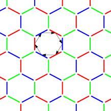
Figure 1: Dynamics of local collective rearrangements (alternating two-color loops of size $l$) satisfying the hard local constraints (no nearest neighbor bond in the same state).

Discrete classical models have no dynamics by themselves, but it is interesting to consider a standard stochastic dynamics which connects states by random local flips.effective In the present context, the only possible moves that are compatible with the constraints consist of an exchange of colors along two-color closed loops (an example is shown in Fig. 1). Note that there are always two loops going through each bond, and the loop lengths are broadly distributed.Chakraborty ; Chandra We assume that flipping a loop is governed by an activation process with a time scale $\tau_{l}=\tau_{0}\exp(\kappa l/T)$, which depends on the length of the loop $l$, but we do not specify the origin of $\kappa$.cepascanals In fact, we further simplify the dynamics and consider various “levels” of dynamics. At each level $l$, only the loops smaller than $l$ may flip. This does not mean that the sites belonging to longer loops never flip, because the neighboring loops reorganize the configuration. The dynamics here is therefore assumed to be local, contrary to previous works.Chakraborty ; Castelnovo

     

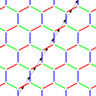
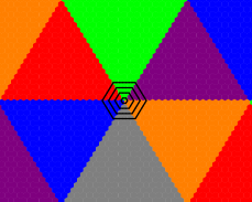
Figure 2: Right: Ground state (in the “zero flux sector”), consisting of six macroscopic mono-domains related by symmetry (one is shown on the left), fitting in the hexagonal shape of the boundaries. While in a mono-domain (left), the loop degrees of freedom are straight and infinite, here they form concentric loops of increasing size (some are shown in black).

We can thus address the issue of the relaxation of the dynamics by the short-scale degrees of freedom. In particular, what is the minimal scale that the system has to nucleate in order to relax and reach a typical state? By including an energy for the configurations, we can study this issue for very different states in the configuration space. It is indeed interesting since the short and long-loop phases are asymmetric with respect to the length of the loops.

We start from initial states in the microcanonical ensemble at any given energy $E$, and compute numerically the autocorrelation function,

$$C_{l}(t)=\frac{1}{N}\sum_{i}\langle S_{i}(t).S_{i}(0)\rangle_{E}$$ (2)

at various scales $l$, i.e., under the stochastic dynamics of all loops up to length $l$. The average $\langle\dots\rangle_{E}$ is done over up to 500 independent initial states in each energy bin $E$. These states are prepared by a Wang-Landau random walk in energy space,WL so as to cover the entire energy range. We use finite-size clusters of hexagonal shape (that has the same symmetries as the infinite lattice) with periodic boundary conditions, and sizes up to $L=30$ for the dynamics ($N=9\times L^{2}$) and $L=26$ for the computation of the density of states. For larger sizes, the density of states does not converge in the entire energy range (with up to $5\times 10^{6}$ Monte Carlo sweeps [MCS] for each Wang-Landau iteration) and we have used smaller energy intervals by starting from special states. When $l$ is large enough, the autocorrelation relaxes to zero from $C_{l}(0)=1$, in a few MCS. For small $l$, we use 200 MCS to allow for convergence (except for $l=6$ and high-energy states $E\sim 2$, where the convergence is much slower and we use $4\times 10^{3}$ MCS).

Since the dynamics is local, we reject in particular the infinite loops that wind around the periodic boundary conditions. As a consequence, the dynamics conserves some topological numbers,Castelnovotopo and we restrict the study to the “zero-flux sector”. This is without loss of generality since the lowest energy state in the zero-flux sector is not the mono-domain $Q=0$ state mentioned above (which is in the highest-flux sector) but consists of six triangular mono-domains, arranged in such a way as to be compatible with the hexagonal shape (see Fig. 2). Its energy per site $E$ is higher by a “surface” energy term, $E-E_{0}=3/L$, that vanishes in the thermodynamic limit. It is interesting to consider the latter since it allows to address the question as to whether it can be connected from a typical state by a local dynamics, whereas the former cannot.

For typical random states of dimer models, the dynamics is generally expected to be diffusive with $C_{l}(t)\sim t^{-\alpha}$ at long times.Henley For the degenerate three-coloring model, this is indeed the case when $l$ is large enough, with an exponent $\alpha=2/3$.cepascanals For smaller values of $l$, we now show that the diffusion is blocked and the autocorrelation saturates to a finite value after some short time,

$$q_{l}=\lim_{t\rightarrow\infty}C_{l}(t).$$ (3)

A finite value of $q_{l}$ indicates an overlap between the initial state and the final state, i.e., a static frozen moment, as in spin-glasses. $q_{l}$ is given in Fig. 3, for different $l$ and as a function of the energy $E$ of the initial state. They increase continuously below energy thresholds that depend on $l$, and reach values close to one at lower energies. The figure shows that the curves collapse approximately onto a single function $f(x)\approx(1+\exp x)^{-1}$ of the rescaled parameter $x=(E-E_{l})/\delta E_{l}$ (solid line in Fig. 3), where $E_{l}$ and $\delta E_{l}$ are given in the inset. Note that for $l=6$ at high-energy, there are some fluctuations in the points resulting from low statistics in this energy range. The collapse shows some self-similarity of the dynamics at different scales.

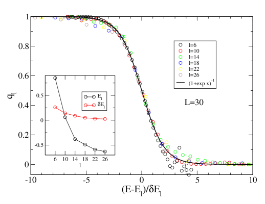
Figure 3: Static moments, $q_{l}=\lim_{t\rightarrow\infty}C_{l}(t)$ for the dynamics including loops up to length $l<l^{*}$, as functions of rescaled energy $x=(E-E_{l})/\delta E_{l}$, with parameters given in the inset. They collapse approximately onto a single curve (solid line).

II.2 Growing barriers and multiple time scales

We define an ergodic or relaxation length scale $l^{*}$ such that $q_{l^{*}}=0$, but $q_{l}\neq 0$ for $l<l^{*}$. Since the loops of length $l^{*}$ have to flip before the system can fully relax, the relaxation time of the system is given by $\tau_{l^{*}}$. In other words, when $q_{l}\neq 0$, the system is trapped into some basin of energy, and moves within smaller basins under the dynamics of loops of length $l<l^{*}$. It is only when the system passes energy barriers of order $l^{*}$ that it escapes its basin into a liquidlike regime.

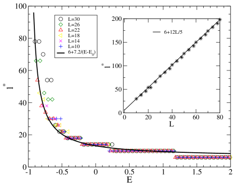
Figure 4: Minimal length $l^{*}$ of loops that need to be included in the dynamics to decorrelate a state with initial energy $E$: $l^{*}$ grows at low energies generating an additional time scale at each step. Inset: Diverging $l^{*}\sim L$ for the ground state (the solid line is exact when $L$ is a multiple of ten).

We have computed $l^{*}$ for the three-color model as a function of the energy of the initial state (Fig. 4), by using the data of Fig. 3. In practice, the thresholds slightly depend on the definition of $q_{l}\neq 0$ (which we have taken to be $q_{l}>0.2$). It is a discontinuous function since the allowed values of $l$ are a multiple of four on this lattice, starting from the smallest hexagonal loops with $l=l_{1}=6$. For the typical random states at $E\approx 1.03$ (corresponding to the maximum of entropy, see Fig. 5), we have $l^{*}=10$, giving two time scales, as shown earlier.cepascanals By reducing the energy further, $l^{*}$ increases to very large values. This corresponds to growing activation barriers in the relaxation time, $\tau_{l^{*}}$. Furthermore, the motion of loops with $l<l^{*}$ reorganizes the system partially (with the values of $q_{l}$ given in Fig. 3), on time scale, $\tau_{l}$. The dynamics is, therefore, characterized by multiple intermediate time scales, the number of which increases with $l^{*}$. The energy landscape becomes more and more hierarchical at low energy with basins within basins.

For the ground state, $l^{*}$ is growing with $L$ (inset of Fig. 4), in particular we find that $l^{*}=l_{1}(1+2L/5)$ (solid line) is exact when $L$ is a multiple of ten, which we explain below. It is therefore diverging in the thermodynamic limit and the ground state cannot be melt in a typical state by local processes. The ground state is truly metastable in this model. For intermediate energies, we find that

$$l^{*}=l_{1}+\frac{\beta}{E-E_{0}}$$ (4)

with $\beta=7.2$, is a rather good approximation in the entire energy range, bare the discreteness of the loop lengths (solid line in Fig. 4). We show that it is exact for all the finite-size ground states. From the numerics, it is not clear whether $l^{*}$ could diverge at an energy $E>E_{0}$. The statistics in averaging $C_{l}(t)$ is low for $E<-0.5$ because it is more difficult to generate independent states in this energy range. We construct in Sec. III.3 some excited states with $E>E_{0}$, where $l^{*}$ is also infinite but they have a finite overlap with the ground state. Nevertheless, Fig. 4 provides a connection between the energy of the system and its dynamics.

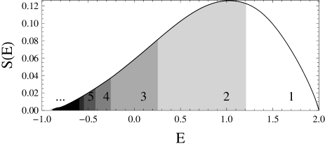
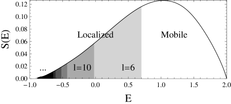
Figure 5: Logarithm of the density of states, $S(E)$, numerically determined by the Wang-Landau algorithm for $L=26$. The number of time scales in the dynamics and their energy thresholds are indicated (top panel), as well as the (classical) “mobility edges” for loops of length $l$ (bottom panel). The maximum of $S(E)$ is 0.1258, very close to Baxter’s result, 0.1264, in the thermodynamic limit.

The behavior of $l^{*}$ can be simply understood for the lowest and highest energy states. First, the state at $E=2$ has all its hexagons flippable: It is therefore clear that $l^{*}=6$. Incidentally, the averaged loop length is also $\langle l\rangle=6$. For the ground state, on the other hand, the two-color loops are straight lines in each mono-domain and form concentric structures around the three special points where all the domains join (see Fig. 2). Their lengths increase as $l_{k}=l_{1}(2k-1)$ with $k=1,\dots,L$ (in particular, the averaged loop length $\langle l\rangle=Ll_{1}$ and the size of each domain are diverging in the thermodynamic limit). However the concentric loops of small sizes create only localized rearrangements in small zones and create no new flippable loop of the same length. It is only when the loop size is of the order of the distance between two such zones that a complete reorganization becomes possible. Since the domains are macroscopic, we therefore conclude that $l^{*}\sim L$. Careful examination of the state shows that $l^{*}=l_{1}(1+2L/5)$ when $L$ is a multiple of ten, as found numerically. Since the ground state has energy $E=E_{0}+3/L$, we may rewrite $l^{*}=l_{1}+\beta/(E-E_{0})$ with $\beta=6l_{1}/5=7.2$, which is precisely Eq. (4). This formula is therefore exact for all the finite-size ground states (when $L$ is a multiple of ten), and is a good approximation in the entire energy range.

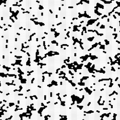
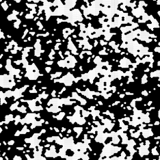
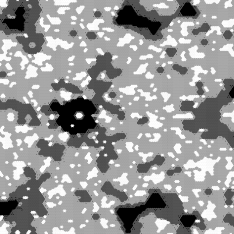
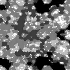
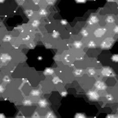
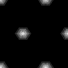
Figure 6: Hierarchies of frozen regions developing from high energy (typical state, top left) to low energy (ground state, bottom right). Each deeper level of gray corresponds to sites that move on a longer time scale $\tau_{l}$ ($l<l^{*}$), i.e., a region insulated from smaller faster loops ($<l$). There are energy thresholds $E_{l}$ for the appearance of time scales and thresholds for the localization (percolation) of the degrees of freedom of length $l$ in isolated pockets (see Fig. 5).

     

     

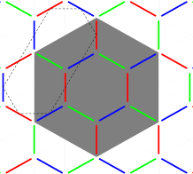
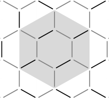
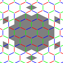
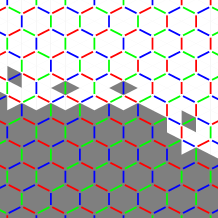
Figure 7: Simple examples of regions insulated from $l=6$ (top left) or $l=10$ (bottom left) degrees of freedom. In the dimer model, there is no insulated cluster (top right). Insulated regions are not necessarily a perfect domain of the long-loop phase (see, for instance, the bottom right figure).

We may now ask whether Eq. (4) is generic for models with long-loop ground states. When the averaged loop length $\langle l\rangle$ and the size of the ordered domains diverge at low energy, does the system necessarily have a diverging $l^{*}$? In order to understand this point, we consider the equivalent dimer model on the hexagonal lattice. It has a similar long-loop phase (staggered phase), which, in the zero-flux sector, has three domains made of the three long-range dimer orientations. By contrast, in this case, we find that $l^{*}=l_{1}$. This happens because flipping the single flippable hexagon located where the three domains meet generates in turn neighboring flippable hexagons which propagate in the entire system. This is very different from the three-color model studied above where flipping the same loop does not generate flippable neighboring loops. The important point is therefore not the density of small loops (a single loop may be sufficient) nor the presence of large domains with a diverging $\langle l\rangle$ but whether these loops are able to reorganize the system on a global scale. We now explain why they cannot in the three-color model.

II.3 Insulated regions

We study how the static moments at the different levels of the dynamics are structured in real space, in frozen regions. In order to do this, we record the spins which do not move within the time of the simulation (the persistent field) on different scales. In Fig. 6, each figure shows a real-space map of the persistent field at different levels $l<l^{*}$ of the dynamics (each level is shown in gray scale) for the same initial state. The figures correspond to different initial states with different energies which range from a typical state (top left) down to the ground state (bottom right). For the typical state, the two time scales are visible, with the fast $l=6$ (in white) and slow $l=10$ (in black) regions. For lower energy states, we see a developing hierarchy of regions, with higher-level regions fully insulated from all shorter loops. Each region at level $l_{0}$ is inaccessible to the loops of length $l<l_{0}$, but not to loops of length $l_{0}$. They are therefore frozen on all time scales, $\tau_{l}$ ($l<l_{0}$), but have some dynamics on the longer time scale $\tau_{l_{0}}$. The origin of this behavior is easy to understand by looking at the configurations.

A region is insulated, when its border is protected from the flippable degrees of freedom, whatever configuration the outside may take in the course of the dynamics. Examples are given in Fig. 7. The simplest example (top left) is a 12-site cluster of sites insulated from the loops of length 6: The central hexagon is not flippable (it is not a two-color loop) and the neighboring hexagons will never be flippable, since they have already three colors on the border. We therefore immediately see that this is not the case for the equivalent (two-color) dimer model (top right): There is nothing that prevents the border from being flippable. The insulated cluster, drawn on top left, is not insulated from loops of length 10 (one is shown by a dashed line). The simplest cluster insulated from loops of length 10 is shown at the bottom left. It has 48 sites and there is no loop of length 6 nor 10 inside or on its border. The smallest flippable one is 14. The simplest cluster insulated from loops of length 14 has one 108 sites, etc. Although all these clusters have the local order of the ground state with long loops, larger insulated regions do not (see an entire region insulated to loops 10 in Fig. 7, bottom right): The insulated regions do not coincide with the domains of the ordered state.

II.4 Percolation of the insulated regions

When the static moment $q_{l}$ becomes large, the corresponding frozen regions also become large and percolate. For example, at $E=0.6$, the frozen regions form an infinite percolating cluster (top right in Fig. 6). We find indeed that the first percolation threshold occurs at $E\sim 0.7$, where $q_{6}=0.64\equiv q_{p}$. The density of frozen sites is $0.44$, smaller than the standard bond-percolation threshold, $0.6527$, on the hexagonal lattice (or site-percolation threshold of the kagome lattice), but there are correlations here and the threshold is a nonuniversal quantity. As a consequence, the $l=6$ degrees of freedom are now localized in some pockets in space, and become more and more localized as the energy further decreases (see Fig. 6). As the energy is lowered, the longer scales also get successively localized and we have a cascade of percolation transitions. We have not computed the precise (classical) “mobility edges” for all scales, and some schematic ones are shown in Fig. 5, simply obtained by using $q_{l}=q_{p}$. For the ground state (bottom right), there is an infinite number of scales up to $l=l^{*}\sim L$, that are localized in the zones shown. Because of this localization, no local scale can rearrange the system globally.

This model therefore provides an example where classical dynamical degrees of freedom get localized in the absence of disorder. This implies, in particular, that the energy injected in a given state cannot diffuse on the time scale $\tau_{l}$ unless the corresponding region at level $l$ percolates.

III Thermal equilibrium and metastability

Among the states of energy $E$ studied above, we can study the most probable states at thermal equilibrium at a temperature $T$. We show below that the system undergoes a first-order phase transition at thermal equilibrium, between a paramagnetic phase and the ground state represented in Fig. 2. However, since we found that the ground state is dynamically unreachable by the local processes we have considered (the system has to pass a macroscopic barrier of order $\sim L$), the ergodicity is broken below $T_{m}$. Depending on thermal preparations, any energy state of the system may be relevant.

III.1 First-order transition at equilibrium

We have computed the equilibrium free-energy $F(E,T)=E-TS(E)$ from $S(E)$ shown in Fig. 5. The logarithm of the density of state $S(E)$ is obtained by the Wang-Landau Monte Carlo algorithm.WL In these simulations, we have flipped the loops irrespective of their sizes, according to the acceptation ratio that makes it possible to reach flat histograms in energy space. We have used a square root reduction of the modification factor at each Wang-Landau step and checked the convergence of $S(E)$. We have obtained the density of states in the entire energy range for $L\leq 26$, but not for larger sizes. We also mention that we could not directly equilibrate the system at low temperatures with the standard loop Metropolis algorithm for $L>20$ (with 10⁶ MCS per temperature). This is, in fact, similar to previous works where the equilibration of long-loop phases in the triangular Ising modelDasgupta or the three-color modelChakraborty ; Castelnovo is not possible for large sizes, even with a nonlocal dynamics.

As a test of the results, we note that the maximum of $S(E)$ obtained for $L=26$ is at $0.1258$, within 0.5% of Baxter’s thermodynamic result, $S_{0}=0.126375$… Simulations in the restricted energy range $[0,2]$ up to $L=40$ leads to a finite-size extrapolation of $0.12628$ or $0.12647$, depending on whether we include a $1/L$ contribution in the fit.

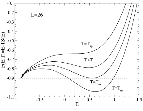
Figure 8: First-order phase transition at thermal equilibrium, obtained from Wang-Landau simulations. There are two minima in the free-energy $F(E,T)=E-TS(E)$ down to $T_{sp}=11.0$ (upper curve; vertical dashed line: $E_{sp}=0.19$), and equal at $T=T_{m}=13.6$ ($L=26$).

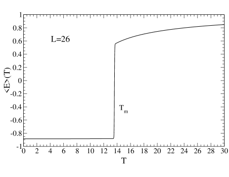
Figure 9: Jump in the internal energy as a function of temperature at the first-order transition, at equilibrium, from Wang-Landau simulations.

In Fig. 8, we show that the free-energy has two minima above a spinodal temperature $T_{sp}=11.0$, where the paramagnetic phase becomes unstable. The two minima have the same free-energy at $T=T_{m}(L=26)=13.6$. Finite-size scaling leads to $T_{m}=14.50$ in the thermodynamic limit. This is the predicted melting temperature where the internal energy of the system $\langle E\rangle(T)$ jumps (see Fig. 9, computed from the density of states by using canonical formulasWL ). The ground state energy is indeed $E=E_{0}+3/L$ as explained above. The simple argument for the first-order transition is that of an attraction between the long loops: Fitting two long loops as nearest neighbors costs twice the boundary energy, whereas fitting them apart costs four times the boundary energy.

III.2 Metastability and absence of critical droplets

The first-order transition takes place, provided that thermal equilibrium can be achieved. As the temperature is lowered below $T_{m}$, the system remains metastable in the supercooled phase down to $T_{sp}$. Its relaxation time is controlled by $\tau_{l^{*}}$, which increases faster than Arrhenius. At $T_{sp}$, we have $\langle E_{sp}\rangle=0.19$ (vertical dashed line in Fig. 8), so that we obtain $l^{*}=14$ from Fig. 4. The enhancement of the energy barrier is only a factor of $14/6$, when the liquid looses its stability. Usually, in a first-order transition, a critical droplet nucleates and grows. Here, this does not take place because the growth of droplets (as evidenced from the growth of $\langle l\rangle$) is accompanied by the growth of $l^{*}$, i.e., a slowing down of the dynamics. There is no critical size of the droplet above which the growth will be fast. For $T<T_{sp}$, the dynamics is out of equilibrium, and the system evolves in the hierarchical energy landscape that we have described, without being able to reach its ground state.

III.3 Linear specific heat due to localized rearrangements

We argue that the localized elementary excitations may give rise to a specific heat that is linear in temperature, in the metastable low-energy states. For this, we first consider the ground state (Fig. 2) and its excited configurations, obtained by flipping loops with $l<l^{*}$, so that the ground state remains mostly frozen, except in some local zones (see Fig. 6 bottom right). We consider a single zone, where each concentric loop with size $l_{k}\sim k$ can be in two states. As long as $l_{k}<l^{*}$ (this implies that $k=1,\dots,p=L/5$ where $p$ satisfies $l_{p+1}=l^{*}$) no new loop with $l<l^{*}$ is generated if a loop flips. There are therefore $2^{p}$ excited configurations that are specified by a set of $p$ integers $\{n_{k}\}$ denoting loops either in their ground state ($n_{k}=0$) or in an excited state ($n_{k}=1$). A single loop excitation with $k>1$ creates two interfaces and costs “surface” energy, $E_{k}\sim k$. Given that the model is short-ranged, there is a short-range interaction between two loops (nearest neighbor), which is an attraction. We find no interaction energy beyond two loops, except for the pairwise attraction. The energy of any of these restricted configurations reads

$$E=\sum_{k=1}^{p}E_{k}n_{k}-\sum_{k=1}^{p-1}(E_{k}+E_{1})n_{k}n_{k+1}$$ (5)

where $E_{k}=3l_{k}$ increases with $k$. If we flip all loops ($n_{k}=1$), we create a new ordered zone (but rotated by 60^o) and this costs only “surface” energy of order $L$. Since $E_{k}$ is linear in $k$, the first term has a contribution in $L^{2}$ (recall that $p\sim L$) which must be canceled by the second term. This explains the general form of the energy, Eq. (5). Note that the highest energy state (with the same diverging $l^{*}$) consists of flipping every other loop up to $p$. It has a finite excess energy per site of $1/25$.

The problem is the same as that of an Ising chain with $p$ sites and open boundary conditions, with a coupling constant which increases linearly with the bond position. Its partition function can be obtained exactly by transfer matrices (but has not as far as we know) and reads

$$Z=\sum_{C}e^{-\beta E}=\prod_{k=1}^{p}(1+x^{k})=\sum_{k=0}^{p(p+1)/2}p_{d}(k)x^{k}$$ (6)

where we have expanded the product as a polynomial of $x=\exp(-\beta E_{1})$. The coefficients $p_{d}(k)$ appear to be the number of partitions of the integer $k$ into distinct summands when $p$ is large enough. $p_{d}(k)$ can be computed exactly and, in the thermodynamic limit ($p\rightarrow\infty$), the asymptotic form reads,AbramowitzStegun

$$p_{d}(k)\sim\frac{1}{k^{3/4}}e^{\pi\sqrt{k/3}}$$ (7)

This is the degeneracy of the energy level $E_{k}=kE_{1}$, and therefore its logarithm is

$$S(E)\equiv\ln p_{d}(k)\sim\pi\sqrt{\frac{E}{3E_{1}}}$$ (8)

If we assume local thermal equilibrium at temperature $T$, we have $\frac{1}{T}=\frac{\partial S}{\partial E}$, leading to $E(T)=\frac{\pi^{2}}{4E_{1}}T^{2}$ for the three independent zones, hence a linear specific heat

$$C=\frac{\pi^{2}}{36}T$$ (9)

The linear dependence is rather unusual in classical systems, but might apply more generally at grain boundaries where localized excitations are. The important point is a linear increase of both the energy and the interaction for longer excitations that both compensate when a new ordered grain is formed [Eq. (5)]. Equation (9) is valid for the metastable ground state at temperatures above the energy gap, $E_{1}$, when many loops (a few in practice) are excited, and up to infinite temperatures (the ground state is metastable), since it is always possible in the thermodynamic limit to find longer loops. Importantly, note that $C$ is nonextensive and we need a finite density of such zones to obtain an extensive quantity. This is typically obtained in a polycrystalline state (see the density of “concentric” structures in Fig. 6, bottom left). In this case, the available loop lengths do not extend to infinity, and there is a maximum in the specific heat determined by the longer loop excited, at a given time scale.

IV Discussion of some analogy with structural glasses

IV.1 General slowing down mechanism

We discuss the hypothesis of Adam and GibbsAG in the view of the present model. We identify the “cooperatively rearranging regions” with the loop degrees of freedom, and the time scale is activated

$$\tau_{l}=\tau_{0}\exp(\kappa l/T),$$ (10)

for each individual rearranging region, a point that we discuss below. Each rearranging region of size $l$ has an entropy

$$s^{*}=\ln\Omega$$ (11)

($\Omega=2$ in the present model). In Adam and Gibbs, the rearranging regions are independent and form $N/l$ domains with $l$ molecules, so that the total entropy is

$$S=\frac{N}{l}s^{*}$$ (12)

A direct consequence of this assumption is that the size $l$ of the smallest cooperatively rearranging region increases as the entropy decreases (the domains grow).

The first essential difference with the present model is that the loop degrees of freedom are not independent: When a loop flips, it reorganizes the neighboring loops which may in turn be flippable. A second difference is that the size of the smallest cooperatively rearranging regions does not grow here: It is always $l=6$ (down to the ground state) and these loops do have dynamics. The point is that they can rearrange some regions locally but may not rearrange the system globally. Moreover, as the domains of the ordered state grow (at low energy), the regions insulated from the small-scale loops not only grow, but also get insulated from larger and larger scales. This gives a different interpretation for growing barriers. Note that the occurrence of growing domains is not sufficient. Indeed, in the dimer model, as we showed, the domains grow but $l^{*}$ does not, because these domains are not insulated. The Adam-Gibbs interpretation does not apply in this case, precisely because there is no way to protect the ordered domains from the cooperatively rearranging regions (which are not independent domains). Adam and Gibbs indeed do not describe why the dynamics is activated with a relaxation time $\tau_{0}\exp(\kappa l/T)$ for an entire domain of $l$ molecules. This is at odds with the dynamics of the dimer model as explained above, but also more simply with the Ising model, where rearranging a domain does not imply an activation energy: The domain walls may move and rearrange the domain on a fast time scale $l^{z}$ (where $z$ is a dynamical exponent). In the context of glasses, a mechanism must then protect the domain from this fast mechanism. The present model gives a solution to this point: No short scales can rearrange the insulated regions because their borders are protected. It is therefore not the number of molecules in the domain that controls the relaxation time, but the size $l^{*}$ of the smallest loops that will rearrange the deepest insulated region. Moreover, the hierarchical structure of these regions gives multiple intermediate time scales, a point which is also evidenced in structural glasses, for example, from the stretched exponential behavior of the relaxation functions, and was phenomenologically described.Palmer

IV.2 Microscopic analogy

The microscopic analogy consists of identifying the chain-like excitations observed in molecular dynamics simulations of structural glassesKob with the present loops. In fact, it was even found that their averaged size grows slightly on lowering the temperature,Kob just as in the present model. They are certainly more complicated because of the structurally disordered environment and their organization in space is not clear.

Pursuing the analogy, we may see (1) the monocrystal as infinite chains (in two spatial dimensions) that cannot rearrange themselves (then the crystal is metastable in absence of dislocations); (2) the supercooled liquid has local collective rearrangements on different scales because the chains are not structurally ordered, and has developed hierarchical insulated regions (which are not crystalline domains); (3) the liquid phase at higher energy has lost the hierarchical structure and can rearrange itself on the shortest time scale. We have distinguished two cases: Either the crystal can be reached by moving elemental loops of a few molecules (as in the two-color dimer model) or not (as in the three-color model). This is reminiscent of the physics of hard discs where the monodisperse particles can form a solid phase but the polydisperse ones generally leads to a glassy phase.

The activated behavior of the individual loops $\tau_{l}=\tau_{0}\exp(\kappa l/T)$ is also assumed in the present work, and we have not specified $\kappa$. The energy barriers may result from (1) a local thermodynamic equilibrium: Flipping a loop increases the energy because of the interactions with the neighboring sites. Alternatively, (2) it may result from an interaction with the long wavelength vibrations. If flipping a loop does not cost any energy (for instance, the local interactions are translationally invariant), such displacements create nevertheless some diffusing potentials for the long-wavelength harmonic oscillations, which may result in preferred positions and barriers between them.cepascanals An important point is the presence of hard local constraints. If the constraint is softened (noninfinite nearest-neighbor coupling $J_{1}$), it is possible to create a pair of defects that can diffuse fast and annihilate.Castelnovo This is equivalent to flipping the loops but it occurs typically on time scale $\tau_{d}\sim l^{2}\exp(J_{1}/T)$. This process is dominant for loops longer than $l>J_{1}/\kappa$, giving a cutoff for the diverging barriers. The activation is therefore relevant only if a strong enough local constraint prevents the nucleation of such defects.

We have identified the equilibrium long-range-ordered phase below $T_{m}$ with the solid phase since it breaks both the translational and the orientational symmetries; and the paramagnetic phase with the liquid which can be supercooled down to $T_{sp}$. The internal energy of the liquid is well defined down to $T_{sp}$. If we assume that it varies as $\langle E\rangle(T)\sim E_{\infty}-C/T$, a Vogel-Fulcher law results from Eq. (4), down to $T_{sp}$. In fact, there is only a discrete increase of the energy barriers ($l^{*}$ is discrete) and their enhancement factor, 14/6 at $T_{sp}$, is relatively small in this model. Below $T_{sp}$, there is no liquid “phase” anymore. The system is out-of-equilibrium and gets stuck into some basin of energy, which depends on the cooling rate. We may imagine that if the cooling is very slow and becomes comparable to $\tau_{d}$, the ground state may be reached, thanks to the defects. It is an interesting issue and the equilibration does not always occur either.Moessner ; Levis

Hard constraints also lead to some features apparently different from standard liquids. The paramagnetic phase does not break any symmetry but has, unlike a true liquid, an infinite correlation length. The correlations are algebraic and therefore a quasi-Bragg peak is expected in the structure factor instead of a broad feature. The quasi-Bragg peak appears at the $Q$ vector corresponding to the $\sqrt{3}\times\sqrt{3}$ unit-cell and is at a different position from that of the solid. It can be seen as a preferred structure in the liquid phase (minimizing the strong local constraint), and this structure is not compatible with long-range orientational order, since it favors short loops. Again, a softening of the hard constraint will generate defects and a finite correlation length.

The linear specific heat found in Sec. III.3 cannot be directly applied to amorphous states at low temperatures, because it is at temperatures above the energy gap, $T>E_{1}$, determined by the smallest loop. Note, however, that the quantum tunneling of the loops that we have not treated here, or a coupling to the bath of long wave-length vibrations, may extend its regime of validity to lower temperatures. Here the model simply assumes some classical interacting two-level systems, with a physical interpretation. They represent localized collective excitations that can reconstruct a new ordered domain locally, and may also be relevant under an external shear. The slope of the specific heat is argued to be proportional to the density of such zones in the limit of small density.

V Conclusion

We have identified a model within which static moments appear when the scales of the dynamical degrees of freedom are smaller than a length scale $l^{*}$ that we have computed. This length scale grows at low energy, providing growing energy barriers in the relaxation of the system. The smaller scales are unable to reorganize the system globally, leaving some insulated regions in space. These regions form a hierarchical structure, and the reorganization of the deeper levels implies multiple time scales in the dynamics. Although the system would undergo a first-order phase transition at thermal equilibrium, we have argued that it gets trapped in the complex energy landscape that we have described.

We have discussed a tentative analogy with structural glasses. The present model gives an interpretation of the assumptions made by Adam and Gibbs to explain the growing barriers. It suggests in particular that we replace the idea of independent domains by that of hierarchical insulated regions, the relaxation of which is controlled by a growing $l^{*}$ rather than its size.

- (1) G. Adam and J. H. Gibbs, J. Chem. Phys. 43, 139 (1965).
- (2) For a recent review, see F. H. Stillinger and P. G. Debenedetti, Annu. Rev. Condens. Matter Phys. 4, 263 (2013).
- (3) C. Donati, J. F. Douglas, W. Kob, S. J. Plimpton, P. H. Poole, and S. C. Glotzer, Phys. Rev. Lett. 80, 2338 (1998).
- (4) J. S. Langer, Phys. Rev. Lett. 97, 115704 (2006).
- (5) B. Chakraborty, D. Das, and J. Kondev, Eur. Phys. J. E 9, 227 (2002).
- (6) C. Castelnovo, P. Pujol, and C. Chamon, Phys. Rev. B 69, 104529 (2004).
- (7) A dynamics can be nonergodic because of conserved quantities. In hard-constrained systems with periodic boundary conditions, topological numbers are conserved when the dynamics is local and excludes infinite winding loops. Another example is given when the dynamics excludes all but the shortest loops. In this case, a Z2 conserved quantity was found in the dimer model on the three-dimensional pyrochlore lattice [O. Sikora, N. Shannon, F. Pollmann, K. Penc, and P. Fulde, Phys. Rev. B 84, 115129 (2011)], or on the cubic lattice [M. Freedman, M. B. Hastings, C. Nayak, and X.-L. Qi, Phys. Rev. B 84, 245119 (2011)].
- (8) For a recent discussion of this point, see G. Biroli and J.-P. Bouchaud, in Structural Glasses and Supercooled Liquids: Theory, Experiments and Applications, edited by P. G. Wolynes and V. Lubchenko (John Wiley and Sons, Hoboken, NJ, 2012); also in arxiv:0912.2542.
- (9) See appendix B in M. Hermele, M. P. A. Fisher, and L. Balents, Phys. Rev. B 69, 064404 (2004).
- (10) R. J. Baxter, J. Math. Phys. 11, 784 (1970).
- (11) L. Pauling, J. Am. Chem. Soc. 57, 2680 (1935); E. H. Lieb, Phys. Rev. 162, 162 (1967).
- (12) O. Cépas and B. Canals, Phys. Rev. B 86, 024434 (2012).
- (13) D. Das, G. Farrell, J. Kondev, and B. Chakraborty, J. Phys. Chem. B 109, 21413 (2005).
- (14) L. Angelani, G. Parisi, G. Ruocco, and G. Viliani, Phys. Rev. Lett. 81, 4648 (1998).
- (15) D. A. Huse and A. D. Rutenberg, Phys. Rev. B 45, 7536 (1992).
- (16) P. Chandra, P. Coleman, I. Ritchey, J. Phys. I France 3, 591 (1993).
- (17) This can be seen as an effective dynamics of the continuous frustrated Heisenberg model,cepascanals which was conjectured to be glassy.Chandra
- (18) F. Wang and D. P. Landau, Phys. Rev. Lett. 86, 2050 (2001).
- (19) For a definition of the topological numbers, see C. Castelnovo, C. Chamon, C. Mudry, and P. Pujol, Phys. Rev. B 72, 104405 (2005).
- (20) C. L. Henley, J. Stat. Phys. 89, 483 (1997).
- (21) A. Dhar, P. Chaudhuri, and C. Dasgupta, Phys. Rev. B 61, 6227 (2000).
- (22) M. Abramowitz and I. A. Stegun, Handbook of Mathematical Functions with Formulas, Graphs, and Mathematical Tables, Ninth printing (Dover Publications, New York), p. 826 (a formula originally due to G. H. Hardy and S. Ramanujan).
- (23) R. G. Palmer, D. L. Stein, E. Abrahams, P. W. Anderson, Phys. Rev. Lett. 53, 958 (1984).
- (24) C. Castelnovo, R. Moessner, S. L. Sondhi, Phys. Rev. Lett. 104, 107201 (2010).
- (25) D. Levis, L. F. Cugliandolo, EPL 97, (3), 30002 (2012).