Towards a public analysis database for LHC new physics searches using MadAnalysis 5
Abstract
We present the implementation, in the MadAnalysis 5 framework, of several ATLAS and CMS searches for supersymmetry in data recorded during the first run of the LHC. We provide extensive details on the validation of our implementations and propose to create a public analysis database within this framework.
pacs:
12.60.-iModels beyond the standard model and 14.80.-jOther particles (including hypothetical)1 Introduction
The LHC was designed as a machine of discovery. It was built to explore the TeV energy scale, in order to unravel the mechanism of electroweak symmetry breaking and shed light on new physics beyond the Standard Model (SM). The recent discovery Aad:2012tfa ; Chatrchyan:2012ufa of a new particle with mass of 125 GeV and properties consistent with the SM Higgs boson is a first triumph for the LHC physics program and has profound implications for our understanding of the universe. We are, however, still left with many fundamental questions open, and to address them it is imperative that the search for new physics continue, at the LHC and elsewhere.
During Run I of the LHC at center-of-mass energies of and 8 TeV, the ATLAS and CMS collaborations have carried out an extensive program searching for new physics in many different channels atlas:susytwiki ; atlas:exoticstwiki ; cms:susytwiki ; cms:exoticstwiki . Since no signal was found, the experimental collaborations interpreted their results setting limits in terms of popular models, such as the CMSSM (Constrained Minimal Supersymmetric Standard Model, see e.g. AbdusSalam:2011fc ), or in terms of so-called Simplified Model Spectra (SMS).111Simplified Models are effective-Lagrangian descriptions involving only a small number of new particles. They were designed as a useful tool for the characterization of new physics, see e.g. Alwall:2008ag ; Alves:2011wf . These searches will be pursued further at higher energies, with first results to be expected soon after the start of Run II in 2015.
There exist, however, many different beyond-the-SM (BSM) theories, and each of them comes with a large variety of concrete realizations. This leads to a multitude of possible scenarios, with complex interrelations between parameters and signatures. It is a challenge for the whole community to work out the implications of the LHC results in the contexts of all these different models, to derive the relevant limits, point out possible loopholes in the current searches, and help design the analyses for the next phase of LHC running at higher energy.
To this end, many groups have been developing private codes for the interpretation of the LHC results. Moreover, recently some public tools became available, which serve the whole community. For the interpretation in the context of Simplified Models, there are SModelS Kraml:2013mwa and Fastlim Papucci:2014rja . SModelS takes the spectrum of any BSM scenario, decomposes it into SMS topologies, and compares it to the cross section upper limits from more than 50 ATLAS and CMS SMS results. Fastlim reconstructs the visible cross sections from pre-calculated efficiency and cross section tables for simplified event topologies, currently taking into account 11 ATLAS analyses which mainly focus on searches for supersymmetric partners of the top and bottom quarks (stops and sbottoms, respectively). For confronting simulated events of any model to LHC results, there is CheckMATE Drees:2013wra . This program currently has 8 ATLAS and 1 CMS supersymmetry (SUSY) analyses implemented, which it re-interprets based on fast simulation. Another tool, XQCAT Barducci:2014ila , is designed specifically for testing scenarios with heavy extra quarks, based on a CMS search for top partners as well as two SUSY searches. Finally, ATOM ATOM is being developed for calculating the efficiencies of signal and control regions of various LHC searches based on the Rivet Buckley:2010ar toolkit.222We note that Rivet Buckley:2010ar itself is designed for unfolded data. Unfolding works very well for SM measurements, and consequently there are many SM analyses from the LHC available on Rivet. For BSM searches with large missing energy however (the typical SUSY case) unfolding is still an open issue. In addition to these stand-alone tools, developed mostly by theorists, one should note the RECAST framework Cranmer:2010hk , which aims at providing a generic platform for requests of re-interpretation of existing analyses; in this case the re-interpretation would be done by the experimental collaboration itself, using the official full simulation software.
In this paper, we follow a complementary approach. We present the implementation of several ATLAS and CMS SUSY analyses in MadAnalysis 5 Conte:2012fm ; Conte:2014zja , with simulation of detector effects based on Delphes 3 deFavereau:2013fsa , and propose to create a public analysis database (PAD) within this framework. MadAnalysis 5 offers a user-friendly platform for collider phenomenology, and the PAD we propose will be easily accessible to and extendible by the whole community. Our proposal is complementary to the existing tools mentioned above in that i) it is based on event simulation, thus avoiding the shortcomings of the Simplified Models approach; ii) the output is the number of events in the different experimental regions of an analysis , which can then be statistically interpreted by the user for a variety of tasks, including limit setting or developing efficiency maps for Simplified Models; and iii) it is a completely Open Source initiative.
In BSM searches, sets of selection criteria are designed in order to maximize the sensitivity to expected signals of new physics. These define so-called signal and control regions, described in the experimental publications. For interpreting a search in the context of a given new physics model, one has to implement these selection criteria together with a description of the detector performance (emulating the various object definitions and efficiencies) in a simulation tool. Based on simulated event samples for the model being tested, the expected number of signal events in the various signal regions (SRs) can then be computed and compared to the number of observed events and the number of expected SM background events, which are reported in the experimental publication.
Non-collaboration members however do not have access to the experimental data, nor the Monte Carlo (MC) event set simulated with an official collaboration detector simulation. This renders the implementation and validation of ATLAS and CMS analyses for re-interpretation of the experimental results in general contexts a tedious task, even more so as the information given in the experimental papers is often incomplete (we will comment more on this in Section 3). We therefore think that a common platform for collecting object definitions, cuts, and all other information necessary to reproduce or use the results of the analyses will be of great value to the high-energy physics community. Moreover, as our project follows an Open Access and Open Data approach, we hope that it will benefit the scientific communication and in particular motivate ATLAS and CMS to provide more information on their analyses, in line with the Les Houches Recommendations oai:arXiv.org:1203.2489 .
The rest of the paper is organized as follows. In Section 2, we briefly recall some new features in MadAnalysis 5, which are pertinent for implementing LHC analyses, and describe the modifications to the Delphes 3 detector simulation which we adopted for this project. In Section 3, we present some ATLAS and CMS analyses which we implemented in the MadAnalysis 5 framework and report in detail on their validation. The relevant C++ codes are all publicly available and may thus constitute the foundation of the PAD. A module for a simplified statistical interpretation of the simulated signals is presented in Section 4. In Section 5 we provide some guidelines, on the one hand for the experimental collaborations regarding what material is needed for a reliable implementation and validation of an analysis, on the other hand for potential contributors to the framework as to how to validate a new analysis implementation. Section 6 contains our conclusions.
2 New developments in MadAnalysis 5 and Delphes 3
2.1 Dealing with multiple signal regions in MadAnalysis 5
In most experimental analyses performed at the LHC, and in particular the searches considered in this work, a branching set of selection criteria (“cuts”) is used to define several different sub-analyses (“regions”) within the same analysis. In conventional coding frameworks, multiple regions are implemented with a nesting of conditions checking these cuts, which grows exponentially more complicated with the number of cuts. The scope of this project has therefore motivated us to extend the MadAnalysis 5 package to facilitate the handling of analyses with multiple regions, as first presented in Brooijmans:2014eja and described in detail in Conte:2014zja .
From version 1.1.10 onwards, the implementation of an analysis in the MadAnalysis 5 framework consists of implementing three basic functions:
-
•
Initialize, dedicated to the initialization of the signal regions, histograms, cuts and any user-defined variables;
-
•
Execute, containing the analysis cuts and weights applied to each event; and
-
•
Finalize, controlling the production of the results of the analysis, i.e., histograms and cut-flow charts.
The new functionalities of MadAnalysis 5 for implementing LHC analyses are described in detail in the new manual of its expert mode Conte:2014zja . To illustrate the handling of multiple regions, we present a few snippets of our implementation ma5code:cms-sus-13-011 of the CMS search for stops in final states with one lepton Chatrchyan:2013xna (see Section 3.1). This search comprises 16 SRs, all of which must be declared in the Initialize function. This is done through the AddRegionSelection method of the analysis manager class, of which Manager() is an instance provided by default with each analysis. It takes as its argument a string uniquely defining the SR under consideration. For instance, two of the 16 SRs of the CMS analysis are declared as
Manager()->AddRegionSelection( "Stop->t+neutralino,LowDeltaM,MET>150"); Manager()->AddRegionSelection( "Stop->t+neutralino,LowDeltaM,MET>200");
The Initialize function should also contain the declaration of selection cuts. This is handled by the AddCut method of the analysis manager class. If a cut is common to all SRs, the AddCut method takes as a single argument a string that uniquely identifies the cut. An example of the declaration of two common cuts is
Manager()->AddCut("1+ candidate lepton");
Manager()->AddCut("1 signal lepton");
If a cut is not common to all regions, the AddCut method requires a second argument, either a string or an array of strings, consisting of the names of all the regions to which the cut applies. For example, an GeV cut that applies to four SRs could be declared as
string SRForMet150Cut[] = {
"Stop->b+chargino,LowDeltaM,MET>150",
"Stop->b+chargino,HighDeltaM,MET>150",
"Stop->t+neutralino,LowDeltaM,MET>150",
"Stop->t+neutralino,HighDeltaM,MET>150"};
Manager()->AddCut("MET>150GeV",SRForMet150Cut);
Histograms are initialized in a similar fashion using the AddHisto method of the manager class. A string argument is hence required to act as a unique identifier for the histogram, provided together with its number of bins and bounds. A further optional argument consisting of a string or array of strings can then be used to associate it with specific regions. The exact syntax can be found in the manual Conte:2014zja .
Most of the logic of the analysis is implemented in the Execute function. This relies both on standard methods to declare particle objects and to compute the observables of interest for event samples including detector simulation Conte:2012fm and on the new manner in which cuts are applied and histograms filled via the analysis manager class Conte:2014zja . In particular, we emphasize the existence of a new isolCones method of the RecLeptonFormat class for testing the isolation of the leptons. This returns a vector of IsolationConeType objects describing the transverse activity in a cone of radius centered on the lepton and whose properties are the following:
-
•
deltaR(): returns the size of the cone;
-
•
ntracks(): returns the number of tracks present in the cone;
-
•
sumPT(): returns the scalar sum of the transverse momenta of all tracks lying in the cone;
-
•
sumET(): returns the scalar sum of the transverse energy deposits in the cone.
In general, experimental analyses only consider tracks with a transverse momentum larger than a given threshold. It should be noted that MadAnalysis 5 does not control this last functionality so that the threshold must be specified at the level of the detector simulator. All these features should be used together with the modifications of Delphes 3 described in the next subsection.
Below we provide a couple of examples for applying cuts and filling histograms. After having declared and filled two vectors, SignalElectrons and SignalMuons, with objects satisfying the signal lepton definitions used in the CMS-SUS-13-011 analysis, we require exactly one signal lepton with the following selection cut:
if( !Manager()->ApplyCut(
(SignalElectrons.size()+SignalMuons.size())>0,
"1+ candidate lepton") ) return true;
The if(...) syntax guarantees that a given event is discarded as soon as all regions fail the cuts applied so far. Histogramming is as easy as applying a cut. For example, as we are interested in the transverse-momentum distribution of the leading lepton, our code contains
Manager()->FillHisto("pT(l)",
SignalLeptons[0]->pt());
This results in the filling of a histogram, previously declared with the name "pT(l)" in the Initialize method, but only when all cuts applied to the relevant regions are satisfied.
Finally, event weights often need to be applied at the analysis level to correct for the efficiency with which physical objects, such as electrons or jets, are identified or likely to trigger the event. In MadAnalysis 5, the weight of an event can easily be modified, if necessary, by using the SetCurrentEventWeight method of the manager class.
After the execution of the program, a set of Saf files (an Xml-inspired format used by MadAnalysis 5) is created. These files are organized in an automatically generated output directory with the same name as the input file (containing the path(s) to the event file(s) to consider), chosen to be input.txt for the sake of the example. At the root of this output directory, one finds a file named in our case input.txt.saf with general information on the analyzed events, such as the associated cross section, the number of events, etc. It comes together with a series of subdirectories named according to the different analyses that have been executed. In the case of an analysis denoted by cms_sus_13_011, the corresponding subdirectory will contain:
-
•
a Saf file cms_sus_13_011.saf listing the names of all the implemented SRs;
-
•
a subdirectory Histograms with a Saf file histos.saf describing all the histograms that have been implemented; and
-
•
a subdirectory Cutflows with a series of Saf files (named according to the definition of the SRs) containing the cut flow tables of all declared SRs.
The structure of the various Saf files is detailed in Conte:2014zja .
2.2 The ‘MA5tune’ of Delphes 3
Delphes deFavereau:2013fsa is a C++ framework dedicated to the simulation of a generic detector such as those used in collider experiments. Contrary to full detector simulation software, Delphes does not simulate the particle-matter interactions, but uses instead a parameterization of the detector response and reconstructs the main physics objects considered in the analyses. This simplified picture results in much faster simulations, while the accuracy level is maintained suitable for realistic phenomenological investigations. From the computing side, Delphes is a modular framework where developers can both add their own contributions and tune the default parameterization according to their needs. This modularity is based on a division of the simulation process into modules inspired by the TTask Root class, and the addition and removal of new elements are easily achievable through a Tcl configuration file. Similarly, the content of the output Root files can be configured at will.
In order to properly recast ATLAS and CMS analyses, a tuning of the version 3 of Delphes has been performed. In the original version of Delphes, an isolation criterion is applied to both leptons and photons, and only particles satisfying this requirement are stored in the output files. We have designed a new Delphes module named CalculationIsolation that allows one to move the isolation requirements in the analysis selection. This module computes several variables useful for the implementation of isolation cuts. Defining cone sizes of and , the number of tracks with a transverse momentum larger than a given threshold, the scalar sum of the transverse momenta of these tracks and the scalar sum of the calorimetric transverse energy deposits lying in the cones are evaluated and saved. In addition, the default module of Delphes dedicated to the filtering of non-isolated lepton and photon candidates is switched off so that all candidates are kept in the output Root files. For consistency reasons, the Delphes module UniqueObjectFinder giving a unique identification to all reconstructed objects is bypassed. Isolation selection cuts can then be performed at the analysis level by means of the isolCones method of the RecLeptonFormat class of MadAnalysis 5, described in the previous subsection and in Conte:2014zja .
Adding the isolation information to the output format yields an increase of the size of the output files. A cleaning of all collections is therefore in order to reduce the file sizes. First, collections such as calorimeter towers and particle-flow objects are not stored. Next, the (heavy) collection of all particles that have been generated at the different level of the simulation chain (hard scattering process, parton showering and hadronization) is pruned. Only particles produced at the hard-scattering process level, as well as final-state leptons and quarks present after parton showering, are stored. In addition, the relations between generated and reconstructed leptons have been retained, together with information on the origin (the mother particle) of each lepton. All these changes result in a reduction of the size of the produced Root files by about a factor of ten when compared to the files produced with the original configuration of Delphes.
This tailored version of Delphes 3, which we internally call Delphes-MA5tune to avoid confusion with the original version, can conveniently be installed locally from the MadAnalysis 5 interpreter by typing in the command
install delphesMA5tune
Even if Delphes 3 is already installed on a given system, one will need this modified ‘MA5tune’ version of the program in order to run the MadAnalysis 5 analyses that we are presenting in this paper. Note however that for the moment MadAnalysis 5 is not able to run with both Delphes and Delphes-MA5tune installed in parallel. This means that the user must take care that only the directory tools/delphesMA5tune (but not the directory tools/delphes) be available in his/her local installation of MadAnalysis 5.
In order to process an (hadronized) event sample with the ‘MA5tune’ of Delphes, it is sufficient to start MadAnalysis 5 in the reconstructed mode, import the considered sample and type
set main.fastsim.package = delphesMA5tune set main.fastsim.detector = cms submit
where cms can be replaced by atlas according to the needs of the user. Default detector parameters are employed and can be modified by the user, following the guidelines displayed on the screen. The output Root file can then be retrieved from the automatically generated working directory.
3 Implemented Analyses and their Validation
To start the analysis database, we have implemented and validated the following ATLAS and CMS SUSY
searches at TeV and an integrated luminosity of about 20 fb-1:
ATLAS:
-
•
Search for stops and sbottoms in final states with no lepton and two -jets Aad:2013ija : ATLAS-SUSY-2013-05;
-
•
Search for charginos, neutralinos and sleptons in final states with two leptons Aad:2014vma : ATLAS-SUSY-2013-11;
CMS:
-
•
Search for stops in the single-lepton final state Chatrchyan:2013xna : CMS-SUS-13-011;
-
•
Search for gluinos and squarks in events with three or more jets and Chatrchyan:2014lfa : CMS-SUS-13-012;
-
•
Search for gluinos in opposite-sign dilepton events, large number of jets, -jets and CMS-PAS-SUS-13-016 : CMS-SUS-13-016.
Several more analyses are currently being implemented and validated.
Below we give some details on these analyses, the level of documentation by the experimental collaboration, and the validation of our MadAnalysis 5 implementations. We begin with the CMS stop search in the single-lepton channel, which also served as our template analysis for developing the extensions of MadAnalysis 5 described briefly in Section 2 and in detail in Conte:2014zja . The related recast code ma5code:cms-sus-13-011 contains extensive comments, which should allow the interested reader to easily use it as template for implementing a different analysis.
A list of all available analyses (which will certainly evolve quickly), instructions on how to use them, as well as more detailed validation notes can be found on the MadAnalysis 5 wiki page ma5wiki . The recast codes themselves are published via Inspire inspire , in order to make them citable (Inspire assigns each submission a DOI doi ) and to ensure that changes can be traced reliably through a rigorous versioning system.
Before proceeding, some general comments are in order. Generally, we cannot reproduce cleaning cuts (for, e.g., cosmic rays and beam effects). Moreover, some basic jet quality criteria must be skipped as we do not have vertex information. This is, however, expected to have a small impact on signal events. In addition, event weights are typically applied by ATLAS and CMS to correct simulated events with respect to data. We take such event weights into account whenever they are available. Otherwise they are neglected and contribute to the overall systematic uncertainty. We note that this uncertainty is expected to be larger when testing signals that are very different from the ones used for the validation, depending on the nature of the reconstructed objects and on the kinematic configuration of the events. In such a case one should interpret the result with care.
Finally, while the selection criteria that define the various SRs are usually clear and well documented, information on the preselection cuts is often missing. In particular, trigger efficiencies, information about isolation, efficiencies for leptons, and the order in which preselection cuts are applied is crucial for reliably reproducing an analysis, but this information is often incomplete in the experimental publications. We hope that this will improve over time and the necessary information will be given systematically either in the physics paper or in a performance note, as also advertised in oai:arXiv.org:1203.2489 .
3.1 CMS-SUS-13-011: search for stops in the single-lepton final state
The CMS search for stops in the single lepton and missing energy, , final state with full luminosity at TeV Chatrchyan:2013xna has been taken as a “template analysis” to develop a common language and framework for the analysis implementation. It also allowed us to test the new developments in MadAnalysis 5 which were necessary for carrying out this project.
The analysis targets two possible decay modes of the stop: and . Since the stops are pair-produced, their decays give rise to two -bosons in each event, one of which is assumed to decay leptonically, whilst the other one is assumed to decay hadronically. In the cut-based version of the analysis,333The search also contains an analysis based on multivariate analysis techniques (MVA); such analyses generically cannot be externally reproduced unless the final MVA is given. As this is not the case so far, we here only use the cut-based version of the analysis. two sets of signal regions with different cuts, each dedicated to one of the two decay modes, are defined. These two sets are further divided into “low ” and “high ” categories, targeting small and large mass differences with the lightest neutralino , respectively. Finally, each of these four categories are further sub-divided using four different requirements. In total, 16 different, potentially overlapping SRs are defined. Two cuts are based on rather complex and specific kinematic variables designed to reduce the dilepton background: a resulting from the full reconstruction of the hadronic top and – a variant of the observable. The implementation of the quantity in our code was straightforward thanks to the C++ Root code provided on the CMS Twiki page. The variable is calculated with the standard MadAnalysis 5 method, see Conte:2014zja , according to the algorithm presented in Bai:2012gs .
Overall, this analysis is very well documented. Some important pieces of information were however missing, in particular the detailed trigger efficiencies and the identification-only efficiencies for electron and muons. These were provided by the CMS collaboration upon request and are now available on the analysis Twiki page cms-sus-13-011-twiki in the section “Additional Material to aid the Phenomenology Community with Reinterpretations of these Results”. In addition, the -tagging efficiency as a function of is not given in the paper, but was taken from Chatrchyan:2013fea . Another technical difficulty came from the isolation criteria. Indeed, the CMS analysis considers the sum of transverse momenta of so-called ‘Particle Flow’ particles in a cone of given . This is difficult to reproduce in our case. Instead, we only use tracks in the inner detector for the isolation. From the two benchmark points for which cut flows are available (see Table 3) we found that a weighting factor of , applied on the events at the same time as the isolation, is sufficient to correct our track-only isolation. Therefore we incorporate this correction to our analysis code.
| benchmark point | CMS result | MA5 result |
|---|---|---|
| benchmark point | CMS result | MA5 result |
|---|---|---|
| GeV | GeV | |||
| cut | CMS result | MA 5 result | CMS result | MA5 result |
| GeV | ||||
| + GeV | ||||
| + | ||||
| + iso-track veto | ||||
| + tau veto | ||||
| + | ||||
| + hadronic | ||||
| + GeV | ||||
| — | — | |||
| — | — | |||
The validation of the reimplementation of the analysis can be done using the eleven benchmark points presented in the experimental paper: four for the “T2tt” simplified model (in which the stop always decays as ), and seven for the “T2bW” simplified model (in which the stop always decays as ), with different assumptions on the various masses. The distributions of the kinematic variables used in the analysis are given in Fig. 2 of Chatrchyan:2013xna after the preselection cuts, with at least one benchmark point for illustration. Also provided are the corresponding histograms after the GeV cut, as supplementary material on the CMS Twiki page cms-sus-13-011-twiki . We use this information, together with the final number of events in the individual SRs (i.e., after all selection cuts) for given benchmark points provided in Tables 4 and 6 of Chatrchyan:2013xna .
The validation material both before and after cuts defining the SRs is truly valuable information since one can separately check on the one hand the implementation of the kinematic variables and the preselection/cleaning cuts, and on the other hand the series of cuts defining the SRs. Furthermore, the large number of benchmark points allows us to check in detail the quality of the reimplementation in complementary regions of phase space.
The validation process was based on (partonic) event samples, in LHE format Boos:2001cv ; Alwall:2006yp , provided by the CMS collaboration. The provision of such event files greatly reduced the uncertainties in the first stage of validation since it avoided possible differences in the configuration of the used Monte Carlo tools. In the case of this CMS analysis, the setup of MadGraph 5 Alwall:2011uj ; Alwall:2014hca —the event generator employed for generating the necessary hard scattering matrix elements—is crucial, in particular with respect to the merging of samples with different (parton-level) jet multiplicities. The LHE files were passed through Pythia 6.4 Sjostrand:2006za for parton showering and hadronization, then processed by our modified version of Delphes 3 (see Section 2.2) for the simulation of the detector effects. The number of events after cuts and histograms produced by MadAnalysis 5 were then normalized to the correct luminosity after including cross sections at the next-to-leading order and next-to-leading logarithmic (NLO+NLL) accuracy Kramer:2012bx , as tabulated by the LHC SUSY Cross Section Working Group 8tevxs_susy .
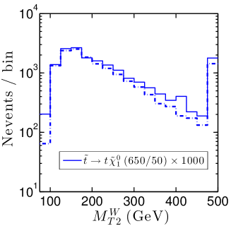
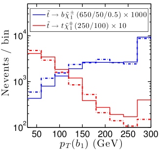
Some examples of histograms reproduced for the validation are shown in Fig. 1. The shapes of the distributions shown – as well as all other distributions that we obtained but do not show here – follow closely the ones from CMS, which indicates the correct implementation of the analysis and all the kinematic variables. (Note that discrepancies in bins where the number of events is relatively small, as seen on a logarithmic scale, suffers from larger statistical uncertainties and hence should not be over-interpreted.) The expected yields for several benchmark points in their relevant SRs are given in Tables 1 and 2. The agreement is good for all tested benchmark points.
Upon our request, the CMS SUSY group furthermore provided detailed cut-flow tables, which are now also available at cms-sus-13-011-twiki . These proved extremely useful because they allowed us to verify our implementation step-by-step in the analysis. A comparison of our results with the official CMS ones is given in Table 3. (Note that here no trigger efficiency or initial state radiation, ISR, reweighting is applied.) For both cases shown, CMS results are reproduced within about 20%. On the whole, we conclude that our implementation gives reasonably accurate results (to the level that can be expected from fast simulation) and declare it as validated. As mentioned, the MadAnalysis 5 code for this analysis, including extensive comments, is published as ma5code:cms-sus-13-011 . More detailed validation material, including extra histograms and validation of the limit-setting procedure (see Section 4), is available at ma5wiki .
3.2 CMS-SUS-13-012: search for new physics through jet multiplicity and missing energy
This CMS search for new physics in the hadronic activity in events with no leptons Chatrchyan:2014lfa targets a number of different signal topologies, in particular:
-
•
gluino-pair production with , denoted as T1qqqq topology in the following;
-
•
gluino-pair production with , denoted as T1tttt;
-
•
gluino-pair production with , followed by , generically denoted as T5VV; and
-
•
squark-pair production with , denoted as T2qq,
following the CMS simplified models naming scheme Chatrchyan:2013sza .
The analysis comprises 36 non-overlapping signal regions, each one defined as a rectangular box volume in the space spanned by the variables , , and . Here is the jet multiplicity of the event, is the scalar sum of the jet transverse momenta, and is the magnitude of the vector sum of the jets transverse momenta. Explicitly,
| (1) |
The event selection was primarily determined from the documentation in Chatrchyan:2014lfa . This document describes six baseline selection criteria on the events, named MET Cleaning, No Lepton, , GeV, GeV, and Min (jets, ). We note that the MET Cleaning cut involves a detailed consideration of spurious signals in the CMS detector, which we cannot simulate with Delphes. Instead, we simply multiply our event count by the efficiency given by CMS. (We stress again that such efficiencies being publicly available is extremely helpful.)
We validated the recast code against cut-flow tables and distributions of the kinematic variables provided by the CMS analysis team as per our request. The benchmark scenarios used are GeV for the T1qqqq, T1tttt and T5VV topologies, and GeV for the T2qq topology, with production cross sections of 10.2 fb and 63.4 fb, respectively Kramer:2012bx ; 8tevxs_susy . For the T5VV topology, one also needs the and masses; they are set to GeV for the GeV benchmark point.
The complete validation material from CMS is available in form of the PDF documents T1qqqq.pdf, T1tttt.pdf, T2qq.pdf and T5VV.pdf in the “Attachments” section on the analysis’ wiki page cms-sus-13-012-twiki . These files correspond to the simplified SUSY models of the same names. For each of the four simplified-model scenarios, the CMS collaboration provided us with events in LHE format along with cut-flow tables and distributions in the variables , , and after each cut. As before, we passed these LHE files to Pythia 6.4 Sjostrand:2006za for showering and hadronization and finally to Delphes for detector simulation. The merging of the partonic events that exhibit different jet multiplicities was performed according to the setup read from the LHE files provided by CMS.
A detail that required additional correspondence with the CMS analysis team were the pseudorapidity () cuts on the electrons and muons used for the lepton veto. We learned that the only requirement on these leptons is that , and they are allowed to reside in the overlap region between the electromagnetic calorimeter barrel and the endcap. We also checked the dependence on the jet energy scale (JES) correction, which is set in the CMS Delphes card, to have good agreement in the , and distributions, and found JES=1.0 to be optimal.
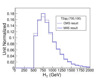
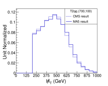
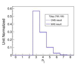
The results of our cut-flow counts for the various simplified models are shown alongside the official counts in Tables 4 and 5. The results were obtained by normalizing with the cross section for each of the benchmark points and for an integrated luminosity of 19.3 fb-1. Moreover, some distributions after the baseline cuts for the case of the T2qq topology are shown in Figs. 2–4. The distributions are normalized to unity and overlaid on the official plots obtained from the collaboration.
The agreement between the official and MadAnalysis 5 results is better than 10% throughout the baseline cut flows. The largest discrepancy arises from the lepton veto cut, which leads to a difference of up to about 5% in the cut flow. The shapes of the distributions qualitatively match very well, and the peaking bins are in accordance with the official results. (This also holds for the other distributions not shown here for space considerations). The MadAnalysis 5 implementation is available as ma5code:cms-sus-13-012 , and a detailed validation note comparing the recast results to the CMS ones can be found at ma5wiki .
| T1qqqq | T1tttt | |||
|---|---|---|---|---|
| cut | CMS result | MA 5 result | CMS result | MA5 result |
| MET Cleaning | 190.6 | 190.6 | 190.5 | 190.5 |
| No Lepton | 190.3 | 190.6 | 95.9 | 101.0 |
| + | 188.1 | 188.5 | 95.8 | 100.9 |
| + GeV | 187.6 | 188.1 | 95.1 | 100.0 |
| + GeV | 158.7 | 159.7 | 75.4 | 81.2 |
| + Min | 130.8 | 131.1 | 62.3 | 66.9 |
| T2qq | T5VV | |||
|---|---|---|---|---|
| cut | CMS result | MA 5 result | CMS result | MA5 result |
| MET Cleaning | 1215.2 | 1215.2 | 189.9 | 189.9 |
| No Lepton | 1212.8 | 1215.2 | 136.2 | 142.1 |
| + | 675.9 | 691.5 | 135.9 | 141.7 |
| + GeV | 619.5 | 638.4 | 135.5 | 141.3 |
| + GeV | 524.0 | 539.6 | 108.8 | 115.2 |
| + Min | 460.7 | 476.1 | 89.6 | 95.2 |
3.3 CMS-SUS-13-016: search for gluinos in events with opposite-sign leptons, -tagged jets and large missing energy
The CMS analysis CMS-PAS-SUS-13-016 searches for new physics in the multi-top final state. The primary target is gluino-pair production followed by , i.e. the T1tttt topology in the CMS simplified-model nomenclature. The dataset used corresponds to a total integrated luminosity of fb-1 at TeV.
The analysis is not published yet but available as a Public Analysis Summary (PAS), which is overall well-documented. The signal selection requires two isolated leptons of opposite sign, a large number of jets, at least three -tagged jets, and large missing transverse energy ( GeV). Moreover, is required for the two leading jets. As there is only one SR, the exclusion is directly obtained from the upper limit on the number of events in the SR.
Let us now turn to our MadAnalysis 5 implementation and its validation. For the lepton isolation, we follow the same procedure as described above for CMS-SUS-13-011 (see Section 3.1). Likewise, the -tagging efficiency as function of is taken from Chatrchyan:2013fea . The most important piece of missing information in this PAS was a cut flow, which was however provided by the collaboration upon request and is now available on the analysis Twiki page cms-sus-13-016-twiki .
Along with the cut flows, CMS provided LHE files corresponding to two benchmark points for the T1tttt simplified model, one with GeV, and one with GeV. The gluino-pair production cross section for these points is 6.7 fb with an uncertainty of 25% Kramer:2012bx ; 8tevxs_susy . Unfortunately, these benchmark points differ by 25 GeV in the neutralino mass from the ones used in the PAS, which have and 500 GeV, respectively. Although this is likely to induce some small differences in the event numbers and distributions, we chose to use the provided LHE files for validation because it avoids more important discrepancies due to differences in the configuration of the MC tools (e.g. the exact version and setup of MadGraph as well as the matching of parton-showers with hard scattering matrix elements and the merging of event samples exhibiting different jet multiplicities).444Note that having the exact same settings of the MC tools is important for purposes of validation. A future user of the recast code, using e.g. a different event generator, may obtain a different result.The LHE files were passed through Pythia 6.4 Sjostrand:2006za for parton showering and hadronization, with the correct merging parameters (given in the LHE files) taken into account. The detector simulation was then performed using the modified version of Delphes, with the -tagging efficiency taken from Chatrchyan:2013fea incorporated in the CMS card. The numbers of events after all cuts were normalized using the cross section information tabulated by the LHC SUSY Cross Section Working Group and for an integrated luminosity of . Our cut flow is compared to the official CMS numbers in Table 6.
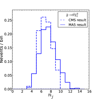
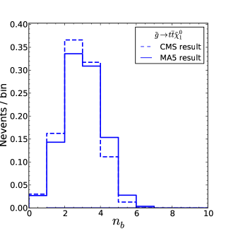
Figures 5–8 show histograms of the kinematic selection variables for the GeV benchmark point. Our MadAnalysis 5 results are overlaid on the official results from Fig. 1 of CMS-PAS-SUS-13-016 , which we digitized. The plots were made by applying all cuts except the one represented, and all the histograms are normalized to unity. We note that the shapes of the distributions are in close agreement with the official ones, with the exception of the distribution, which is slightly shifted towards higher jet multiplicity. Note also that the CMS histogram is cut off at , while the distribution in fact extends to higher .
| GeV | GeV | |||
|---|---|---|---|---|
| cut | CMS result | MA 5 result | CMS result | MA5 result |
| + GeV | ||||
| + | ||||
| + | ||||
| + | ||||
| + | ||||
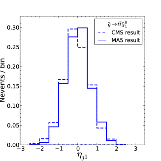
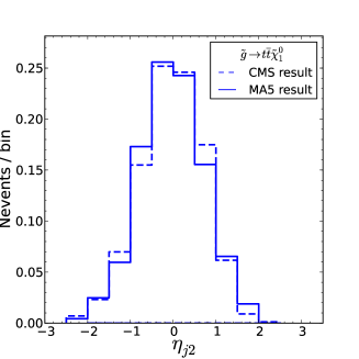
These differences can be attributed to various factors, one of which is the jet energy scale and resolution, for which a 8% uncertainty is quoted in CMS-PAS-SUS-13-016 . Our results shown here were obtained with the JES parameter set to in the CMS Delphes card. A change of this parameter to does not change the results significantly, while a change to changes the final event count by 5 after all cuts, and brings our distribution closer to the official one. Additionally there can be effects like pile-up or jet–lepton separation, which we cannot simulate reliably in this fast-simulation framework. Therefore we regard these effects as systematic uncertainties in our implementation.
Our final numbers of events for the two benchmark points agree within about 20% with the official CMS numbers, see Table 6. This is well within the 17–39% systematic uncertainty given in CMS-PAS-SUS-13-016 . Moreover, the individual cut efficiencies do not differ by more than 8% for any cut for either of the benchmark points. This leads us to conclude that this implementation is well validated. The MadAnalysis 5 code for this analysis is available as ma5code:cms-sus-13-016 and a detailed validation note is available on ma5wiki .
3.4 ATLAS-SUSY-2013-05: search for third-generation squarks in final states with zero leptons and two -jets
In this ATLAS analysis Aad:2013ija , stops and sbottoms are searched for in final states with large missing transverse momentum and two jets identified as -jets. The results are presented for an integrated luminosity of fb-1 at TeV. Two possible sets of SUSY mass spectra were investigated in this analysis:
-
•
sbottom pair production with , and
-
•
stop pair production with , where the subsequent decay of the is invisible due to a small mass splitting with the .
Two sets of SRs, denoted by SRA and SRB, are defined to provide sensitivity to the kinematic topologies associated with the two sets of mass spectra. SRA targets signal events with large mass splittings between the squark and the neutralino by selecting two hard -jets, while SRB is designed to enhance the sensitivity when the squark–neutralino mass difference is small by selecting a hard jet coming from ISR and two softer -jets.
| GeV | GeV | |||
|---|---|---|---|---|
| cut | ATLAS result | MA 5 result | ATLAS result | MA5 result |
| GeV filter | ||||
| + Lepton veto | ||||
| + GeV | ||||
| + Jet Selection | ||||
| + GeV | ||||
| + GeV | ||||
| + GeV | ||||
| + GeV | ||||
| + GeV | ||||
| GeV | GeV | |||
|---|---|---|---|---|
| cut | ATLAS result | MA 5 result | ATLAS result | MA5 result |
| GeV filter | ||||
| + Lepton veto | ||||
| + GeV | ||||
| + Jet Selection | ||||
| + GeV | ||||
For both SRs, events are selected by requiring a large amount of missing transverse energy, GeV, and any event containing an identified muon or electron is vetoed. For the SR selections, all jets with a pseudorapidity are ordered according to their , and two out of the selected jets are required to be -tagged.
In the SRA, the first two leading jets must be -tagged. The event is vetoed if any additional central jet () with GeV is found. To reject the multijet background, large and are required.555 is the minimum azimuthal distance between any of the three leading jets and the vector; is the scalar sum of the of the leading jets and the , with for SRA and for SRB. To reduce the SM background, a cut on the invariant mass of the -jet pair, GeV, is applied. As a final selection, five different thresholds on the contransverse mass Tovey:2008ui ranging from 150 GeV to 350 GeV are demanded to reduce backgrounds from top-quark production.666This peculiar kinematic variable is not yet implemented as a standard method in MadAnalysis 5. We thus used the public code computing this quantity, including the correction due to ISR, available at http://projects.hepforge.org/mctlib.
In SRB, the sensitivity to small squark-neutralino mass difference is increased by selecting events whose leading jet has a very large , which is likely to have been produced by ISR, recoiling against the squark-pair system. High thresholds on the leading jet and on the missing transverse momentum, which are required to be almost back-to-back in , are imposed. The leading jet is required to be non--tagged and two additional jets are required to be -tagged. Just like for SRA, large values of and are required, thereby suppressing the multijet background. The selection for SRB is finally completed by demanding that the additional hadronic activity is bounded from above, GeV. Here, is defined as the scalar sum of the of the jets, without including the three leading jets.
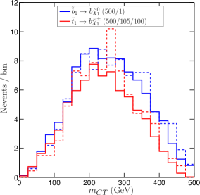
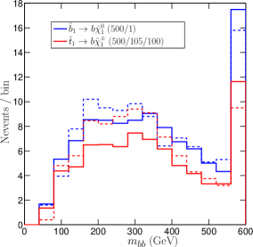
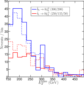
The analysis is very well documented regarding physics, but for recasting purposes more information than provided in the physics paper Aad:2013ija and on the analysis Twiki page atlas-sus-13-05-twiki was needed. Indeed this made the validation of the recast code seriously difficult in the earlier stages of the project. Since then, fortunately, two cut-flow tables were made public. Moreover, the ATLAS SUSY group provided us with general SUSY Les Houches Accord (SLHA) Skands:2003cj input files which we used to simulate the signal, as well as with the exact versions of the MC tools used to generate the SUSY samples, which were not given in Aad:2013ija . When we simulated the signal samples with Madgraph 5 1.4.8 Alwall:2011uj ; Alwall:2014hca and Pythia 6.4 Sjostrand:2006za , we introduced nonetheless additional sources of uncertainties since the complete MC configuration which was used for the signal simulation in ATLAS was not known. For example, the run card for MadEvent Maltoni:2002qb would be precious information. Also, we are missing information on the trigger only and -tagging efficiencies.
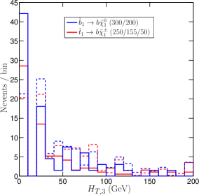
The comparison between the official cut flows and the ones obtained within MadAnalysis 5 are presented in Tables 7 and 8. The numbers were normalized to fb-1 of data using the cross sections tabulated by the LHC SUSY Cross Section Working Group Kramer:2012bx ; 8tevxs_susy . Overall the agreement is quite satisfactory, considering the expected accuracy for a fast simulation. We observe the largest discrepancy in Table 8 in the final number of events in SRB after the cut for the benchmark point = GeV. This discrepancy will also be exhibited in the histogram of the distribution. In the analysis paper Aad:2013ija there are four histograms of distributions that we can compare against. For SRA, there are histograms of and of . Two benchmark points are considered, = GeV and = GeV, which are different from those used for the cut flows. There are also two such distributions for SRB, the distribution and the missing transverse energy . The corresponding benchmark points are = GeV and = GeV.
As far as the SRA distributions are concerned, see Fig. 9, the agreement between our recast analysis and the official one is very good.
The situation is less satisfactory in the SRB case. As already pointed out regarding the cut flow of Table 8, the treatment of the variable seems problematic; we indeed observe a large excess of events in the very first bin of its distribution with respect to the official result from ATLAS. The very first bin corresponds to events where there are no additional jets ( GeV) except the ones which are required to select the event. The second bin is empty since jets are required to have GeV. This shows that, after detector simulation, we do no get enough jet activity. One possible explanation for this might be that we do not account for pile-up effects. According to private communication with ATLAS, the discrepancy is however too large to be accounted for by the pile-up only. Varying the JES by a fixed factor does not improve much the situation for the very first bin but can lead to improvement in the next bins of the distribution. However this also has an impact on the distribution, which gets significantly modified. A possible solution might be a parameterization of the JES in terms of the of the jets for these signal regions, since for low it may vary significantly. In any case, in Aad:2013ija , the JES uncertainty was carefully estimated and amounts to only 3% in SRB. Last but not least, it appears that, at the calorimeter level, Delphes undersmears jets (and thus MET) compared to ATLAS.777We thank Jamie Tattersall for pointing this fact out. Therefore the distribution of soft jets is too sharp and the hadronic activity is reduced too much by the GeV cut. Moreover, for such jets with low the QCD uncertainties are substantial. To investigate the issue more deeply, a more detailed cut flow apportioning the “Jet selection” line in Table 8 would be helpful.
We conclude that for SRA the agreement is quite good. For SRB the efficiency of the cut differs from the official analysis by about 20%, which is acceptable from a fast-simulation viewpoint. Moreover, according to Barnard:2014joa the sensitivity of SRB is difficult to reproduce while the analysis is generally dominated by SRA, as can also be seen in Fig. 3 of the auxiliary figures of atlas-sus-13-05-twiki . Overall this leads us to conclude that this implementation is validated to the best that could be done. The recast code is available as ma5code:atlas-susy-2013-05 , and a detailed validation note can be found on ma5wiki .
3.5 ATLAS-SUSY-2013-11: search for charginos, neutralinos and leptons in di-lepton final states
We consider the ATLAS search for the electroweak production of charginos, neutralinos and sleptons in final states with two leptons (electrons and muons) and missing transverse momentum based on fb-1 of data at 8 TeV Aad:2014vma . The event selection requires two signal leptons of opposite charge, with GeV and GeV. Two kind of final states are considered: same flavor (SF = or ) and different flavors (DF = ).
Three types of signal regions are defined in this analysis. First, the and signal regions require the invariant mass of the lepton pair to be outside the window, and jets are vetoed. The signal regions (SR ) target direct slepton-pair production and chargino-pair production followed by slepton-mediated decays. Each signal region is defined by its threshold on the (“stransverse mass”) variable Lester:1999tx ; Cheng:2008hk that is used for reducing the and backgrounds: , and GeV, for SR-, SR-, and SR-, respectively. The implementation of this requirement is straightforward as the variable is available as a standard method in MadAnalysis 5.
Next, the a, b and c signal regions (referred to as SR-) are designed to provide sensitivity to production followed by leptonic decays. Each of these three regions is optimized for a given kinematic configuration, using cuts on the invariant mass and/or transverse momentum of the slepton pair ( and , respectively), possibly combined with cuts on and on the “relative missing transverse momentum” . Here, is defined as the missing transverse momentum multiplied by of the azimuthal angle between the direction of and that of the closest lepton or jet, , is below . This modified aims at suppressing events where missing transverse momentum is likely to come from mis-measured jets and leptons.
Finally, the jets signal region (SR-jets) targets production, followed by and , with hadronic and leptonic decays. Unlike in the other regions, jets are not vetoed; instead at least two central “light” jets (non--tagged with ) are required. In addition to being consistent with leptonic decays, requirements are made on , , on the invariant mass of the two leading jets () and on the separation between the two leptons () in order to suppress, in particular, the + jets background.
All signal regions separately consider SF and DF leptons, except SR-jets where only SF leptons are considered. In total, 20 potentially overlapping signal regions are defined (considering and signal regions separately, as required for comparison with the official ATLAS cut flows). Detailed electron efficiencies as a function of and are available in ATLAS-CONF-2014-032 ; we used the electron efficiencies as a function of for , while muon efficiencies were taken to be 100% as a good approximation. The analysis is very well-documented and gives clearly the various preselection criteria and signal region cuts. Moreover, an effort was made in the definition of the tested new physics scenarios: a whole section of the experimental publication is dedicated to the description of the different SUSY scenarios. Furthermore, SLHA files were uploaded to HepData atlas-susy-11-hepdata in May 2014 after discussion with the ATLAS SUSY conveners.
For validation, at least one cut-flow table is given for every signal region and type of scenario tested, which is very good practice. In addition, several histograms are given and can be used to validate the distribution of, in particular, and . Finally, regarding the interpretations in terms of simplified models, not only the information on the 95% confidence level (CL) upper bound on the visible cross section is given, but also the CLs value, which is useful for validation of the limit-setting procedure. The only difficulty came from the benchmark points for direct slepton production. Given the SLHA files provided on HepData, it was not clear whether the slepton masses given as in the cut-flow charts and histograms really correspond to the physical masses or to the slepton soft terms. The difference can be of several GeV, inducing some uncertainty in the kinematic distributions and in the production cross sections for these scenarios.
Event samples used for the validation were generated with Herwig++ 2.5.2 Bahr:2008pv , using as input the SLHA files provided on HepData. For each of the nine benchmark points we considered, events were generated. In the case of chargino-pair production, non-leptonic decays of the intermediate -boson were filtered to increase statistics. Similarly, for chargino–neutralino production, non-leptonic decays of the intermediate -boson were filtered. The cross sections for the benchmark points, evaluated at the NLO+NLL accuracy Fuks:2012qx ; Fuks:2013vua ; Fuks:2013lya , were taken from the HepData entry.
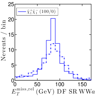
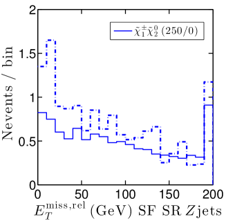
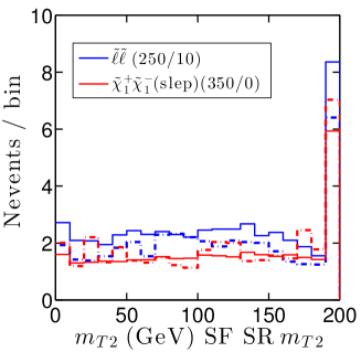
Tables 9–11 give some examples of cut flows for different benchmark points and signal regions, comparing the results obtained with our MadAnalysis 5 implementation to the official ATLAS numbers. (The complete list of cut flows for all nine benchmark points is available at ma5wiki .) We systematically find the jet veto to be less efficient than it should be, but did not find any explanation for this effect. This was also noted in Drees:2013wra . Still, reasonably good agreement is observed for the available benchmark points. Distributions of , and in some signal regions are shown in Figs. 11 and 12. Good agreement is observed. Note that the fluctuations in the ATLAS results in the left panel of Fig. 12 may correspond to statistical fluctuations and/or uncertainties when digitizing the ATLAS histogram (the results are extracted from a logarithmic scale that spans over six orders of magnitude).
We conclude that our MadAnalysis 5 implementation of ATLAS-SUSY-2013-11 reproduces well the experimental results. Our C++ code for this analysis is published as ma5code:atlas-susy-2013-11 ; complete validation materials including validation of the limit-setting procedure (see next section) can be found at ma5wiki .
| cut | ATLAS result | MA5 result |
|---|---|---|
| Initial number of events | ||
| 2 OS leptons | ||
| GeV | ||
| veto | ||
| leptons | ||
| jet veto | ||
| veto | ||
| GeV | ||
| GeV | ||
| GeV |
| cut | ATLAS result | MA5 result |
|---|---|---|
| Initial number of events | ||
| 2 OS leptons | ||
| GeV | ||
| veto | ||
| leptons | ||
| central light jets | ||
| and forward jet veto | ||
| window | ||
| GeV | ||
| GeV | ||
| GeV | ||
| GeV |
| cut | ATLAS result | MA5 result |
|---|---|---|
| Initial number of events | ||
| 2 OS leptons | ||
| GeV | ||
| veto | ||
| leptons | ||
| jet veto | ||
| veto | ||
| GeV |
4 Limit setting
For the statistical interpretation of the results, we provide on ma5wiki a Python code, exclusion_CLs.py, for computing exclusions using the prescription Read:2002hq .888The Python code requires SciPy libraries to be installed. This code can also be installed on a user system by typing in, from the MadAnalysis 5 interpreter, the command
install RecastingTools
which results in the file exclusion_CLs.py being present at the root of any working directory created in the expert mode of MadAnalysis 5. We refer to Conte:2014zja ; ma5wiki for details on the creation of MadAnalysis 5 working directories.
The exclusion_CLs.py code takes as input the acceptance efficiency information from the cut flow Saf files generated when executing an analysis implemented in MadAnalysis 5 (see Section 2.1). Moreover, an Xml file, named analysis_name.info (where analysis_name stands for a generic analysis name), needs to be provided by the user in the Build/SampleAnalyzer/User/Analyzer directory, specifying the luminosity <lumi>, the number of observed events <nobs>, the nominal number of expected SM background events <nb>, and its uncertainty at 68% CL <deltanb> in each of the regions, as given in the experimental publication. The syntax of this file is as follows:
<analysis id="cms_sus_13_011">
<lumi>19.5</lumi> <!-- in fb^-1 -->
<region type="signal" id="SRname">
<nobs>227</nobs>
<nb>251</nb>
<deltanb>50</deltanb>
</region>
...
...
</analysis>
The attribute type of the root tag <analysis> can be signal or control and is optional (the default value is signal). The id of each <region> tag has to match the exact name of the SR used in the analysis code. When results are given after combining several SRs (for example, for same-flavor leptons instead of and separately), the relevant SRs should all be listed in the attribute id separated by semicolons (without extra space). Taking the example of the ATLAS analysis presented in Section 3.5, this would read
<region id="MT2-90 ee;MT2-90 mumu">
The last piece of information essential for calculating exclusions is the signal cross section. It can be provided by the user in the Saf file mypoint.txt.saf (automatically generated when executing an analysis, see Section 2.1), where mypoint.txt, stored in the Input folder of the working directory, is the input file for running the analysis under consideration. Alternatively, the cross section can be given as argument when calling exclusion_CLs.py. Concretely, the limit-setting code is called as
./exclusion_CLs.py analysis_name mypoint.txt \
[run_number] [cross section in pb]
where the run number and cross section value are optional arguments. The run number (default zero) identifies the output directory to use, as each execution of the analysis code yields the creation of a new output directory, analysis_name_, for the execution of the analysis code (starting from 0).
The procedure of exclusion_CLs.py starts by selecting the most sensitive SR (i.e., the one that yields the best expected exclusion, assuming that the number of observed events is equal to the nominal number of background events). This is a standard procedure at the LHC whenever the SRs defined in the analysis are overlapping; here we use it as the default for all analyses. Then the actual exclusion is calculated, and the confidence level with which the tested scenario is excluded using the prescription Read:2002hq is printed on the screen together with the name of the most sensitive SR. The same information is also stored in the file analysis_name_.out, located in the working directory of the Output folder. Last but not least, if a negative number is given for the cross section, the code returns instead the nominal cross section that is excluded at 95% CL, computed using a root-finding algorithm.
The core of the calculation works as follows. First, the number of signal events () is obtained as the product of the luminosity, signal cross section and acceptance efficiency for the SR of interest. This is used, together with the number of observed events () and the nominal number of background events () and its uncertainty () to compute the exclusion. A large number of toy MC experiments ( by default) are then generated from the Poisson distribution , corresponding to the distribution of the total number of events in the SR under the background-only hypothesis on the one hand (), and under the signal background hypothesis () on the other hand. We assume that the uncertainty on the number of background events is modeled as , and for each toy MC the number of background events is randomly generated from this normal distribution. Under the two different hypotheses, -values are then calculated using the number of events actually observed at the LHC, and finally used to compute the value.
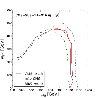
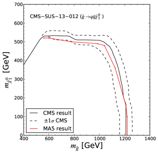
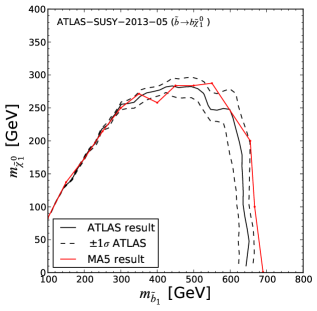
We have tested the limit-setting code on the analyses presented in this paper and generally found good agreement with the official exclusions from ATLAS and CMS. Figures 13–15 give some illustrative examples. In particular, Fig. 13 shows the 95% CL exclusion limit in the neutralino versus gluino mass plane for the topology reproduced with the MadAnalysis 5 implementation ma5code:cms-sus-13-016 of CMS-SUS-13-016. This analysis has only one SR and thus provides a good test for our implementation of the prescription. To prove that our procedure also works well for analyses with many SRs, Fig. 14 shows the 95% CL exclusion limit for the topology (T1qqqq) reproduced with the MadAnalysis 5 implementation ma5code:cms-sus-13-012 of CMS-SUS-13-012. We also find good agreement for the T1tttt and T5VV topologies for this analysis; the one case that works less well is the T2qq topology (squark-pair production with ) for which the reproduced limit becomes unreliable for neutralino masses above about 200–250 GeV. For improving the situation, the statistical model for combining the SRs would be needed from CMS, but this is not available. Finally, Fig. 15 shows the 95% CL exclusion limit in the neutralino versus sbottom mass plane for pair production with reproduced with the MadAnalysis 5 implementation ma5code:atlas-susy-2013-05 of ATLAS-SUSY-2013-05 and compared to the official ATLAS limit. This is the case where the largest differences are encountered in the kinematic distributions, see Section 3.4. None the less we see that the limit is reasonably well reproduced (note that the uncertainty quoted by ATLAS is based only on the theory uncertainty of the cross section).
Last but not least it is important to note that the module exclusion_CLs.py is intended only as a lightweight tool for the user who wants an approximate but fast evaluation of the results of his/her simulation. Users who want to go beyond the simplifications made in exclusion_CLs.py are encouraged to use e.g. the RooFit and RooStats machinery rooCLs adopted by ATLAS and CMS.
5 Guidelines
In this section, we provide some brief guidelines, on the one hand for the experimental collaborations regarding what material is needed for a reliable implementation and validation of an analysis, on the other hand for potential contributors to the framework as to how to validate a new analysis implementation.
5.1 Information needed from the experiments
The information needed from the experimental collaboration on an analysis splits into two parts: analysis description and material for validation. We ask the collaborations to provide
1. in the analysis description:
-
•
a clear and unambiguous definition of all the cuts and the sequence in which they are applied;
-
•
efficiencies as function of (and, where relevant, ) for all physics objects considered in the analysis: electrons, muons, taus, -jets, light jets, etc.;
-
•
efficiencies for triggers and event cleaning.
At present, cuts are typically well defined, but their sequence is not always clear. A clear ordering in tabulated form or by means of detailed cut flows would help. Efficiencies are sometimes only roughly indicated, which is very problematic for us; if an efficiency is not given explicitly in the paper, it should be clearly referenced where to find it (e.g. pointing to the precise figure in a performance note).
Efficiencies for triggers and event cleaning are of particular concern, as they are highly important for our purpose but currently often missing altogether in the experimental papers.
2. as validation material:
-
•
unambiguously defined benchmark points, e.g. in the form of SLHA files (including the full mass spectrum and decay tables) and/or parton-level MC event files;
-
•
exact configuration of MC tools: the ideal would be if the run cards and input scripts for MadGraph, Pythia, etc. were made available; if this is not the case, we need at least the exact versions of the MC tools and their basic settings;
-
•
detailed cut flows for all benchmark points, showing each step of the analysis;
-
•
histograms of kinematic distributions after specific cuts.
Only if complete information is provided for an analysis can the recasting be done in a reliable way. In this respect is should also be noted that for any analysis in which SRs are combined the corresponding likelihood model should be made available by the collaboration.
Some more comments are in order. First, we note that code modules for special kinematical variables, as currently provided by CMS, are extremely useful. We highly appreciate this practice. Second, we note that having to read efficiencies, event numbers or other data off paper plots is very tedious and introduces unwarranted uncertainties, especially when dealing with log-scale plots. We therefore strongly encourage the collaborations to always provide their plots also in numerical form, be it on HepData or on the analysis Twiki page. Finally, one could also imagine that the experimental collaborations directly provide validated MadAnalysis 5 implementations for certain analyses. While this would be an excellent way of documenting an analysis, this is of course left to the initiative and decision of the respective search groups.
5.2 Recommendations for implementing and validating new analyses
Since the framework we presented here is intended as an open-source project, we also give some guidelines for potential contributors:
-
•
clearly identify and reference the analysis together with your contact details in the header of the recast code;
-
•
always implement all SRs of an analysis;
-
•
take care that the code is clean and well commented;
-
•
reproduce all the cut flows provided by the experimental collaboration for the various benchmark points;
-
•
reproduce all the available kinematic distributions for the benchmark points;
-
•
for the above, use the exact same settings of the MC tools as the experimental collaboration;
-
•
if information for any of the above is missing, contact the experimental collaboration;
-
•
likewise, contact the experimental collaboration if not enough validation material is available, e.g. if cut flows are not detailed enough;
-
•
the required agreement with the experimental results is somewhat analysis dependent — generally, we think it should be of the order of 30% or better for the final numbers as well as in each step of the cut flow; if larger discrepancies are found, contacting the collaboration can be helpful for resolving them;
-
•
while we think that cut flows and kinematical distributions should be the primary validation material, it is also a good idea to reproduce the 95% CL limit curve for the relevant simplified model(s);
-
•
publish your code via Inspire inspiresubmission ;
-
•
provide a detailed validation note to be put on ma5wiki .
6 Conclusions
We have presented a new scheme for developing and deploying implementations of LHC analyses based on fast simulation within the MadAnalysis 5 framework. This can serve to create a public analysis database, which may be used and developed further by the whole community. The codes for the five analyses ma5code:cms-sus-13-011 ; ma5code:cms-sus-13-012 ; ma5code:cms-sus-13-016 ; ma5code:atlas-susy-2013-05 ; ma5code:atlas-susy-2013-11 that we published together with this paper are intended as a starting point for this database and may conveniently be used as templates for other analyses.
We propose that the C++ codes of new implementations within this scheme be published via Inspire inspiresubmission , as done here, best together with the physics paper they have been developed for. This way, each analysis implementation is assigned a Digital Object Identifier (DOI) doi , ensuring that it is uniquely identifiable, searchable and citable. In addition it is very useful if a detailed validation note is made available on the MadAnalysis 5 wiki page ma5wiki .
The ease with which an experimental analysis can be implemented and validated may serve as a useful check for the experimental collaborations for the quality of their documentation. Note, finally, that the platform we are proposing might also be used by the experimental collaborations to directly provide implementations of their analyses for fast simulation, thereby assuring the maximum usability of their results, as for example envisaged in level 1 of the CMS statement on “data preservation, re-use and open access policy” CMS:DataPolicy .
It is important for the legacy of the LHC that its experimental results can be used by the whole high-energy physics community. We hope that our project contributes to this aim.
Acknowledgements
We thank our experimental colleagues, in particular Alessandro Gaz, Benjamin Hooberman, Christian Sander, Niki Saoulidou, Nadia Strobbe, Keith A. Ulmer, Frank Würthwein from CMS, as well as Jamie Boyd, Marie-Helene Genest and Monica d’Onofrio from ATLAS for help in the validation process and for providing additional information where needed. Moreover, we thank Daniel Schmeier and Jamie Tattersall for extremely useful discussions. This work originated from the 2013 Les Houches “Physics at TeV Colliders” workshop; the inspiring and open-minded atmosphere of this workshop has been crucial for this project.
Partial financial support by the French ANR projects 12-BS05-0006 DMAstroLHC and 12-JS05-002-01 BATS@ LHC, the Theory-LHC-France initiative of CNRS/IN2P3, and the “Investissements d’avenir, Labex ENIGMASS” is gratefully acknowledged. S.B. thanks the LPSC Grenoble for hospitality.
References
- (1) ATLAS Collaboration, G. Aad et al., “Observation of a new particle in the search for the Standard Model Higgs boson with the ATLAS detector at the LHC,” Phys.Lett. B716 (2012) 1–29, 1207.7214.
- (2) CMS Collaboration, S. Chatrchyan et al., “Observation of a new boson at a mass of 125 GeV with the CMS experiment at the LHC,” Phys.Lett. B716 (2012) 30–61, 1207.7235.
- (3) https://twiki.cern.ch/twiki/bin/view/AtlasPublic/SupersymmetryPublicResults.
- (4) https://twiki.cern.ch/twiki/bin/view/AtlasPublic/ExoticsPublicResults.
- (5) https://twiki.cern.ch/twiki/bin/view/CMSPublic/PhysicsResultsSUS.
- (6) https://twiki.cern.ch/twiki/bin/view/CMSPublic/PhysicsResultsEXO; https://twiki.cern.ch/twiki/bin/view/CMSPublic/PhysicsResultsB2G.
- (7) S. AbdusSalam, B. Allanach, H. Dreiner, J. Ellis, U. Ellwanger, et al., “Benchmark Models, Planes, Lines and Points for Future SUSY Searches at the LHC,” Eur.Phys.J. C71 (2011) 1835, 1109.3859.
- (8) J. Alwall, P. Schuster, and N. Toro, “Simplified Models for a First Characterization of New Physics at the LHC,” Phys.Rev. D79 (2009) 075020, 0810.3921.
- (9) LHC New Physics Working Group Collaboration, D. Alves et al., “Simplified Models for LHC New Physics Searches,” J.Phys. G39 (2012) 105005, 1105.2838.
- (10) S. Kraml, S. Kulkarni, U. Laa, A. Lessa, W. Magerl, et al., “SModelS: a tool for interpreting simplified-model results from the LHC and its application to supersymmetry,” Eur.Phys.J. C74 (2014) 2868, 1312.4175.
- (11) M. Papucci, K. Sakurai, A. Weiler, and L. Zeune, “Fastlim: a fast LHC limit calculator,” Eur.Phys.J. C74 (2014) 11, 3163, 1402.0492.
- (12) M. Drees, H. Dreiner, D. Schmeier, J. Tattersall, and J. S. Kim, “CheckMATE: Confronting your Favourite New Physics Model with LHC Data,” Comput.Phys.Commun. 187 (2014) 227, 1312.2591.
- (13) D. Barducci, A. Belyaev, M. Buchkremer, G. Cacciapaglia, A. Deandrea, et al., “Model Independent Framework for Analysis of Scenarios with Multiple Heavy Extra Quarks,” JHEP 1412 (2014) 080, 1405.0737.
- (14) I.-W. Kim, M. Papucci, K. Sakurai, and A. Weiler, “ATOM: Automated Testing Of Models,” to appear.
- (15) A. Buckley, J. Butterworth, L. Lonnblad, D. Grellscheid, H. Hoeth, et al., “Rivet user manual,” Comput.Phys.Commun. 184 (2013) 2803–2819, 1003.0694, http://rivet.hepforge.org.
- (16) K. Cranmer and I. Yavin, “RECAST: Extending the Impact of Existing Analyses,” JHEP 1104 (2011) 038, 1010.2506; http://recast.perimeterinstitute.ca
- (17) E. Conte, B. Fuks, and G. Serret, “MadAnalysis 5, A User-Friendly Framework for Collider Phenomenology,” Comput.Phys.Commun. 184 (2013) 222–256, 1206.1599.
- (18) E. Conte, B. Dumont, B. Fuks, and C. Wymant, “Designing and recasting LHC analyses with MadAnalysis 5,” Eur.Phys.J. C74 (2014) 10, 3103, 1405.3982.
- (19) J. de Favereau, C. Delaere, P. Demin, A. Giammanco, V. Lemaitre, et al., “DELPHES 3, A modular framework for fast simulation of a generic collider experiment,” JHEP 1402 (2014) 057, 1307.6346.
- (20) S. Kraml, B. Allanach, M. Mangano, H. Prosper, S. Sekmen, et al., “Searches for New Physics: Les Houches Recommendations for the Presentation of LHC Results,” Eur.Phys.J. C72 (2012) 1976, 1203.2489.
- (21) G. Brooijmans, R. Contino, B. Fuks, F. Moortgat, P. Richardson, et al., “Les Houches 2013: Physics at TeV Colliders: New Physics Working Group Report,” 1405.1617.
- (22) B. Dumont, B. Fuks, and C. Wymant, “MadAnalysis 5 implementation of CMS-SUS-13-011: search for stops in the single lepton final state at 8 TeV,” doi: 10.7484/INSPIREHEP.DATA.LR5T.2RR3.
- (23) CMS Collaboration, S. Chatrchyan et al., “Search for top-squark pair production in the single-lepton final state in pp collisions at = 8 TeV,” Eur.Phys.J. C73 (2013) 2677, 1308.1586.
- (24) ATLAS Collaboration, G. Aad et al., “Search for direct third-generation squark pair production in final states with missing transverse momentum and two -jets in 8 TeV collisions with the ATLAS detector,” JHEP 1310 (2013) 189, 1308.2631.
- (25) ATLAS Collaboration, G. Aad et al., “Search for direct production of charginos, neutralinos and sleptons in final states with two leptons and missing transverse momentum in collisions at 8 TeV with the ATLAS detector,” JHEP 1405 (2014) 071, 1403.5294.
- (26) CMS Collaboration, S. Chatrchyan et al., “Search for new physics in the multijet and missing transverse momentum final state in proton-proton collisions at = 8 TeV,” JHEP 1406 (2014) 055, 1402.4770.
- (27) CMS Collaboration, “Search for supersymmetry in pp collisions at sqrt(s) = 8 TeV in events with two opposite sign leptons, large number of jets, b-tagged jets, and large missing transverse energy,” Tech. Rep. CMS-PAS-SUS-13-016, CERN, Geneva, 2013.
- (28) http://madanalysis.irmp.ucl.ac.be/wiki/PhysicsAnalysisDatabase.
- (29) http://inspirehep.net/, see also http://www.projecthepinspire.net/.
- (30) http://www.datacite.org.
- (31) Y. Bai, H.-C. Cheng, J. Gallicchio, and J. Gu, “Stop the Top Background of the Stop Search,” JHEP 1207 (2012) 110, 1203.4813.
- (32) https://twiki.cern.ch/twiki/bin/view/CMSPublic/PhysicsResultsSUS13011.
- (33) CMS Collaboration, S. Chatrchyan et al., “Search for new physics in events with same-sign dileptons and jets in pp collisions at =8 TeV,” JHEP 1401 (2014) 163, 1311.6736.
- (34) E. Boos, M. Dobbs, W. Giele, I. Hinchliffe, J. Huston, et al., “Generic user process interface for event generators,” hep-ph/0109068.
- (35) J. Alwall, A. Ballestrero, P. Bartalini, S. Belov, E. Boos, et al., “A Standard format for Les Houches event files,” Comput.Phys.Commun. 176 (2007) 300–304, hep-ph/0609017.
- (36) J. Alwall, M. Herquet, F. Maltoni, O. Mattelaer, and T. Stelzer, “MadGraph 5: Going Beyond,” JHEP 1106 (2011) 128, 1106.0522.
- (37) J. Alwall, R. Frederix, S. Frixione, V. Hirschi, F. Maltoni, et al., “The automated computation of tree-level and next-to-leading order differential cross sections, and their matching to parton shower simulations,” JHEP 1407 (2014) 079, 1405.0301.
- (38) T. Sjostrand, S. Mrenna, and P. Z. Skands, “PYTHIA 6.4 Physics and Manual,” JHEP 0605 (2006) 026, hep-ph/0603175.
- (39) M. Kramer, A. Kulesza, R. van der Leeuw, M. Mangano, S. Padhi, et al., “Supersymmetry production cross sections in collisions at TeV,” 1206.2892.
- (40) https://twiki.cern.ch/twiki/bin/view/LHCPhysics/SUSYCrossSections.
- (41) CMS Collaboration, S. Chatrchyan et al., “Interpretation of Searches for Supersymmetry with simplified Models,” Phys.Rev. D88 (2013), no. 5, 052017, 1301.2175.
- (42) https://twiki.cern.ch/twiki/bin/view/CMSPublic/PhysicsResultsSUS13012.
- (43) S. Bein and D. Sengupta, “MadAnalysis 5 implementation of CMS-SUS-13-012,” doi: 10.7484/INSPIREHEP.DATA.83GG.U5BW.
- (44) https://twiki.cern.ch/twiki/bin/view/CMSPublic/PhysicsResultsSUS13016.
- (45) D. Sengupta and S. Kulkarni, “MadAnalysis 5 implementation of CMS-SUS-13-016,” doi: 10.7484/INSPIREHEP.DATA.ZC3J.646F.
- (46) https://atlas.web.cern.ch/Atlas/GROUPS/PHYSICS/PAPERS/SUSY-2013-05/.
- (47) D. R. Tovey, “On measuring the masses of pair-produced semi-invisibly decaying particles at hadron colliders,” JHEP 0804 (2008) 034, 0802.2879.
- (48) P. Z. Skands, B. Allanach, H. Baer, C. Balazs, G. Belanger, et al., “SUSY Les Houches accord: Interfacing SUSY spectrum calculators, decay packages, and event generators,” JHEP 0407 (2004) 036, hep-ph/0311123.
- (49) F. Maltoni and T. Stelzer, “MadEvent: Automatic event generation with MadGraph,” JHEP 0302 (2003) 027, hep-ph/0208156.
- (50) J. Barnard and B. Farmer, “A simple technique for combining simplified models and its application to direct stop production,” JHEP 1406 (2014) 13, 1402.3298.
- (51) G. Chalons, “MadAnalysis 5 implementation of ATLAS-SUSY-2013-05,” doi: 10.7484/INSPIREHEP.DATA.Z4ML.3W67.2.
- (52) C. Lester and D. Summers, “Measuring masses of semiinvisibly decaying particles pair produced at hadron colliders,” Phys.Lett. B463 (1999) 99–103, hep-ph/9906349.
- (53) H.-C. Cheng and Z. Han, “Minimal Kinematic Constraints and ,” JHEP 0812 (2008) 063, 0810.5178.
- (54) ATLAS Collaboration, “Electron efficiency measurements with the ATLAS detector using the 2012 LHC proton-proton collision data,” Tech. Rep. ATLAS-CONF-2014-032, CERN, Geneva, June, 2014.
- (55) http://hepdata.cedar.ac.uk/view/ins1286761/
- (56) M. Bahr, S. Gieseke, M. Gigg, D. Grellscheid, K. Hamilton, et al., “Herwig++ Physics and Manual,” Eur.Phys.J. C58 (2008) 639–707, 0803.0883.
- (57) B. Fuks, M. Klasen, D. R. Lamprea, and M. Rothering, “Gaugino production in proton-proton collisions at a center-of-mass energy of 8 TeV,” JHEP 1210 (2012) 081, 1207.2159.
- (58) B. Fuks, M. Klasen, D. R. Lamprea, and M. Rothering, “Precision predictions for electroweak superpartner production at hadron colliders with Resummino,” Eur.Phys.J. C73 (2013) 2480, 1304.0790.
- (59) B. Fuks, M. Klasen, D. R. Lamprea, and M. Rothering, “Revisiting slepton pair production at the Large Hadron Collider,” JHEP 1401 (2014) 168, 1310.2621.
- (60) B. Dumont, “MadAnalysis 5 implementation of ATLAS-SUSY-2013-11: di-leptons plus MET,” doi: 10.7484/INSPIREHEP.DATA.HLMR.T56W.2
- (61) A. L. Read, “Presentation of search results: The CLs technique,” J.Phys. G28 (2002) 2693–2704.
- (62) http://root.cern.ch/root/html/tutorials/roostats/index.html
- (63) http://inspirehep.net/help/data-submission
- (64) CMS Management, “CMS data preservation, re-use and open access policy,” CMS Document 6032-v1.