Density Adaptive Parallel Clustering

Abstract

In this paper we are going to introduce a new nearest neighbours based approach to clustering, and compare it with previous solutions; the resulting algorithm, which takes inspiration from both DBscan and minimum spanning tree approaches, is deterministic but proves simpler, faster and doesn’t require to set in advance a value for $k$, the number of clusters.

1 Introduction

Unsupervised learning is the branch of machine learning that deals with finding hidden structure in data; while supervised learning uses previous information about a labeling of a training set to estimate the labeling value for new input, data in unsupervised learning have yet to be labeled or “classified”.

Approaches to unsupervised learning include:

• clustering, also referred to as cluster analysis;

• blind signal separation using feature extraction techniques for dimensionality reduction (e.g., principal component analysis, independent component analysis, non-negative matrix factorization, singular value decomposition). Acharyya [2008]

• Neural network models, like self-organizing map (SOM) and adaptive resonance theory (ART).

In clustering, the goal is to divide data points into homogeneous subsets, called clusters, such that objects in the same subset or cluster are more similar (according to a specific measure) to each other rather than to those in other subsets.

Many clustering algorithms have been proposed during the years, some more efficient than others, but it is difficult to define an objective definition of what a good cluster should be, and the decision about which of these algorithm to use deeply depend on the characteristics of the data set to be partioned.

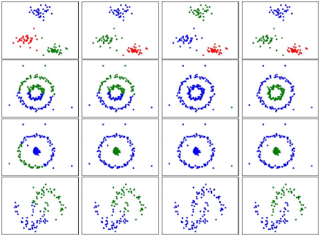
Figure 1: Comparison of k-Means (left), MeanNN (center left), single link (center right) and ITM (right) on four synthetic datasets, as shown in Müller et al. [2012]

2 Related Work

Most clustering algorithms can be categorized based on their cluster model, although not every clustering algorithm provide a model for their clusters; some of the most important categories are:

• Centroid-based clustering: clusters are represented by a central point, which may not necessarily be a member of the data set. Since this optimization problem is known to be NP-hard, the common approach is to search only for approximate solutions. The most commonly used centroid-based clustering algorithm is Lloyd’s algorithm, usually referred to as the k-Means algorithm Lloyd [1982]; MacQueen et al. [1967]; k-Means often works well in practice, but its main limitation is the restriction in cluster shape, that is always forced to be convex. One method that overcomes this limitation is spectral clustering Ng et al. [2002]; Shi and Malik [2000], which solves a graph partitioning problem on a similarity graph based on the data, and hence its performance is heavily affected by the particular choice of graph construction and similarity measure.

• Hierarchical, or connectivity based, clustering: based on the core idea of objects being more related to nearby objects than to objects farther away. These algorithms connect ”objects” to form ”clusters” based on their distance. A cluster can be described largely by the maximum distance needed to connect parts of the cluster. The main downside for these algorithms is their asynthotic running time, which for the simplest methods results $O\left(n^{3}\right)$; more sophisticated methods, like SLINK Sibson [1973] and CLINK Defays [1977], have a worst case running of $O\left(n^{2}\right)$.

  • MST-based clustering: it’s a subset of hirarchical clustering, and it’s been an important filed of research for decades, since 1969 Gower and Ross paper on single-link agglomerative clustering Gower and Ross [1969], a minimum spanning tree-based approach in which the largest edge is removed until the desired number of components is reached. This criterion is further studied by Zahn Zahn [1971]: in his work, only edges that are longer than other edges in the vicinity are cut, although this approach requires tuning several constants by hand. More recently, Grygorash et al. Grygorash et al. [2006] proposed a hierarchical MST-based clustering approach that iteratively cuts edges, merges points in the resulting components, and rebuilds the spanning tree, while in 2012 Muller et al. Müller et al. [2012] proposed an efficient algorithm that infers cluster memberships by direct optimization of a non-parametric mutual information estimate between data distribution and cluster assignment.

• Distribution-based clustering: Distributional clustering, works only under the assumption that the distribution of the data is known explicitly (for example as word counts), which is often not the case in practical situation. Later, in 2005, Banerjee et al. Banerjee et al. [2005] introduced the concept of Bregman Information, generalizing mutual information of distributions, and showed how this leads to a natural formulation of several clustering algorithms. Barber Barber and Agakov [2005] constructs a soft clustering by using a parametric model of conditional probability, and the framework of mutual information based clustering was recently extended to non-parametric entropy estimates by Faivishevsky and Goldberger Faivishevsky and Goldberger [2010]. They use a nearest neighbor based estimator of the mutual information, called MeanNN, that takes into account all possible neighborhoods, therefore combining global and local influences.

• Density-based clustering: clusters are defined as areas of higher density than the remainder of the data set. Objects in these sparse areas - that are required to separate clusters - are usually considered to be noise and border points. The most popular density based clustering method is DBSCAN Ester et al. [1996], which (similarly to linkage based clustering) works by connecting points within certain distance thresholds, the only difference being that it only connects points that satisfy a density criterion. An interesting property of DBSCAN is that its complexity is fairly low - it requires a linear number of range queries on the database - and it is deterministic in nature (except for border points), hence it doesn’t have to be run multiple times. OPTICS Ankerst et al. [1999] is a generalization of DBSCAN that removes the need to choose an appropriate value for the range parameter, and produces a hierarchical result related to that of linkage clustering. DeLi-Clu Achtert et al. [2006], Density-Link-Clustering, combines ideas from single-linkage clustering and OPTICS, eliminating the parameter entirely and offering performance improvements over OPTICS by using an R-tree index for nearest neighbours search. The key drawback of DBSCAN and OPTICS is that they expect some kind of density drop to detect cluster borders. Moreover they can not detect intrinsic cluster structures which are prevalent in the majority of real life data. A variation of DBSCAN, EnDBSCANRoy and Bhattacharyya [2005] efficiently detects such kinds of structures.

An increasingly crucial issue is performance: the rise of big data led to a need to process larger and larger data sets, which in turn led to an increasingly tendency to trade semantic meaning of the generated clusters for performance. To cope with this need, pre-clustering methods such as canopy clustering McCallum et al. [2000] were introduced to process huge data sets efficiently, even if the resulting ”clusters” are merely a rough pre-partitioning of the data set, and those partitions need to be analyzed in a later step with the existing slower methods above.

3 A new approach, inspired by the past

Our solution has been inspired by both DBScan and MST approaches; while the first one is very fast and well performing, it requires a bit of tuning for each dataset because two parameters need to be set, a threshold and the radius of the scanning area; MST based approaches, on the other hand, achieves better results with ill-shaped clusters [see figure 1]Müller et al. [2012], but it is so slow to be unpractical for moderately large base of data (more than 10K elements).

Noticing the flaws of the MST solution, we decided to try to gain the same benefits using a different way to improve performance. The key observation is that, if we are going to apply Kruskal algorithm to build the MST of an “euclidean” graph, i.e. a fully connected graph of points in the plane, where edge weight coincides with Euclidean distance, at each step the shortest path between a vertex in the cut and a vertex outside the cut, is the edge connecting the two of them, and the shortest cut-edge is the one among cut and non-cut vertices with the smallest distance.

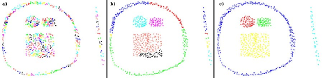
Figure 2: Clusting resulting from the naive nearest neighbour approach, with differents value for parameter $m$ (respectively $m=1$, $m=2$, $m=3$)

With this in mind, the first, naive, approach would obviously be to scan every point in the dataset and merge its cluster with it’s nearest neighbour’s one; to perform this operation quickly we decide to use SS+Trees Kurniawati et al. [1997] for nearest neighbours computation, and weighted UnionMerge with path compression to keep track of the elements’ clusters (see an analysis of the running time below). However, the result was not particularly encouraging, and it is not difficult to see why: most points are each other nearest neighbours, so we end up with a high fragmentation, due to a lot of very small clusters as you can see in the example from figure [Figure 2a].

By incrementing $m$, the number of nearest neighbours considered for each data point, the results improves dramatically, as you can see in [Figure 2b] ($m=2$) and [Figure 2c] ($m=3$): the clustering of this particular datasets looks just right, and this version of algorithm already succeeds even where k-means and NN-mean are forced to failure by their own nature as shown in [Figure 3].

However, even this improved version has a flaw. Consider the dataset in [Figure 4]: a single point $z$ has been strategically added to the dataset in [Figure 3], so that it is approximately at the same distance from blue and red clusters; this in turn means that the two closest points to the newly added one, denoted as $x_{z}^{r}$ and $x_{z}^{g}$, lie one in the red cluster, and one in the green one. Therefore, when $z$ is examined, first its cluster $c_{z}$, which at that point only contains $z$ itself, will be merged with $x_{z}^{r}$’s one, creating a new cluster $\hat{c_{z}}$, and then $\hat{c_{z}}$ will be merged with $x_{z}^{g}$’s cluster, so that $x_{z}^{r}$ and $x_{z}^{g}$ will land in the same cluster, as shown in [Figure 4a]. This problem is not new for clustering algorithms: it is commonly known as the single-link effect, and will affect every dataset with dense clusters and some sparse points, especially if they are approximatively equidistant from 2 dense clusters. As a generalization, this unwanted merge of what should be separate clusters will be caused by chains of $j$ sparse points liyng at the same approximate distance from 2 dense clusters, when the smoothing parameter $s\geq j+1$ [Figure 4b].

There is no way to solve this problem by tuning the smoothing parameter, so we needed an alternative approach.

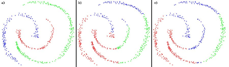
Figure 3: Comparison between 3-nearest neighbours algorithm (a) and kmeans (b) and meann NN (c) algorithms with $n\_cluster=3$

4 An improved version

The previous algorithm performs very well on most datasets, with a little bit of tuning. However, tuning becomes incresingly complicated as the number of points in the dataset grows, and it perniciously shows the tendency to merge together well separated clusters, if a few noise points lies between them. Nonetheless, it represents a fast alternative when noise in the data set is very low.

We knew, however, that - at the cost of some performance - there existed a better solution.

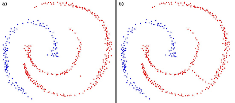
Figure 4: Single link effect on the naive clustering algorithm

What the naive algorihtm was lacking is a way to discriminate noise or, to put it another way, to rule out points too far from our potential clusters.

There were many ways to try to do so - for example running a noise detection algorithm as a first step, and ignore those points identified as noise in our main algorithm.

Instead, we decided to take inspiration from DBscan Ester et al. [1996], a breaktrough in clustering algorithms. DBscan considers two points $p$ and $q$ to be part of the same cluster if they aren’t further apart than a certain distance $\varepsilon$ and if either $p$ or $q$ is surrounded by at least $m$ points; such points are called density-reachable. The idea behind DBscan is the following: for each point $p$, scan an area of radius $\varepsilon$ around $p$, and if at least $m$ points are found in that area, all those points are density-reachable from p, and so they belong to the same cluster. This also implies that if there are two points $p,\,w$ such that there is a sequence $p=p_{1},\>p_{2},\,...\,,\>p_{n}=w$ where $p_{i+1}$ is density-reachable from $p_{i},\>\forall i=1...\>n-1$, then $p$ and $w$ are in the same cluster; such points are called density-connected, and all density-connected points belong to the same cluster.

While DBscan shows several advantages in comparison to k-means (it can find clusters of any shape, it deals with noise and the number of clusters doesn’t need to be set a priori), there are three main problems with DBscan:

1. Both $\varepsilon$ and $m$ are input parameters for DBscan, so they must be decided by the user in advance, and a fair amount of tuning might be needed to get both of them right;

2. It doesn’t scale well to higher dimentional data; [besides it requires either $O\left(n^{2}\right)$ time or space]

3. If the dataset has areas with very different density, then it works very poorly on at least one of them, since it is impossible to find a good compromise for the values of $\varepsilon$ and $m$ that works for all the densities.

Our goal is to introduce the concept of density-reachablility in our naive algorithm, but in an adaptive way, such that the $\varepsilon$ and $m$ parameters are inferred independently for each single point in the dataset, in order to cope with areas with great differences in their density, while still being able to spot and discard noise.

We ended up with an approach similar to DeLi-CluAchtert et al. [2006], with a two steps algorithm: first it scans the dataset, creating a pre-clustering partition, and then for each subset in this partition, estimate a suitable value for the radius $\varepsilon$ of the area to scan to look for neighbours, and uses it in a DBscan alike step.

In particular, during the second phase, for each point with at least $m$ neighbours within its scan area, all its neighbours inside the radius of the area will end up in the same cluster as the point itself. To efficiently perform these two operations, we decided to use SS+trees Kurniawati et al. [1997] for spatial queries, and UnionFind structures to keep track of the clusters: initially every point it’s a cluster of its own, then clusters keep being merged as similarities between points are discovered.

These choices bring several advantages, especially as performance is concerned. As a matter of fact, as we already suggested in the introduction section, a critical problem with modern large dataset is performance, due to the huge amount of data that has to be processed.

Using the UnionFind approach allows a map reduce strategy: we can divide the data space into (slightly overlapping) regions, compute the clustering for each of these regions (map step) and then merge the set resulting from the union find algorithm for each point over the regions in which it appears (reduce step). Each region can thus be assigned to a different processor, since no shared data structure is needed, and reduction can be performed incrementally, as new nodes pubblish their results, so the computation can support a high degree of parallelization. The additional advantage in such a strategy is of course that we can use different parameters for each of these regions, taking into account differences in density as no algorithm could before, and also that UnionFind and SS+trees can run and be computed on a smaller set of points: at the cost of a little space overhead due to the overlapping nature of the regions, the total performance sensibly improves as the number of regions grow.

The key point, of course, is how to find these regions in the first place. If, from a computational point of view, a naive partitioning in regular, same-sized regions could work just as fine, our final goal is to devise the partitioning such that it helps us to cope with possible difference in density. The best approach turned out to be using pre-clustering, in particular step 1 consist of applying canopy clustering McCallum et al. [2000] on the complete data set with an approximate metric to fastly compute the partioning, then compute the $\varepsilon$ parameter based on the points in each partition, and finally build regions for step 2 around these partitions (tipically the smallest box or sphere containing the partition, with at least $m$ points).

As shown by Apache Mahout project (https://cwiki.apache.org/confluence/display/MAHOUT/Canopy+Clustering), canopy clustering support a high degree of parallelization and map reduce strategies as well, since every node can run indipendently.

Another relevant problem is the dimentionality curse: again, SS+trees do scale better than R-trees considering both wasted space (reduced by using spheres instead of boxes) and efficiency (improved by computing an approximation to the smallest enclosing sphere - whose computation is exponential in the number of dimentions).

The final algorithm can be summarized in the following steps:

• First step, run canopy clustering to compute

  pre-clusters,dividing the problem around these

  partitions;

• Second step [Map], process each partition

  separately;

• Third step [Reduce], merge the sets of the union find algorithm for each vertex produced by step 2.

5 Performance

There are four different sub-algorithms contributing to the total running time of the clustering algorithm:

1. Canopy clustering algorithm performance will be strongly dependent on the choice of the metric; our goal is to keep this step as close to $O\left(n\right)$ as possible;

2. The creation of a SS+Tree, which for $k$ points require $O\left(k\,\log k\right)$ time; it also require $O\left(k\right)$ extra space to retain the information;

3. For each point:

   1. A query to find all the points within the scanning area is executed; this search operation is certainly $\Omega\left(\log k\right)$, because that’s the lower bound for a nearest neighbour search on a SS+tree, but it can also be as bad as $O\left(k\right)$ in the worst case, because if the area is big enough it could include all the points in the data set. Typically, however, the area radius is chosen so that a small number of points ($m$ on average, where $m$ is the smoothing parameter defined above) will be included in the scanning area, so small it can considered constant on average, so the average running time for each search operation is $O\left(\log k\right)$;

   2. The UnionMerge procedure will be executed for every one of its neighbours within the scanning area, so, on average, it will be called $m$ times; the average running time of $m$ UnionMerge operation with union rank and path compression is $O\left(m\,\alpha\left(k\right)\right)$, where $\alpha\left(n\right)$ is the inverse Ackerman function, that grows so slowly that it can be considered lower than 5, and so constant, for any practical value of $n$.

   3. The UnionFind data structure used in step (b) requires $O\left(k\right)$ time time to be built and $O\left(k\right)$ extra space;

4. Therefore, the total running time of the second step is

   $O\left(mk\,\alpha\left(k\right)+k\,\log k\right)$

   for $k$ points, which - if $m$ is constant - becomes

   $O\left(k\,\alpha\left(k\right)+k\,\log k\right)=O\left(k\,\log k\right)$.

Without the map reduce parallelization strategy, the SS+tree and UnionFind structure will be constructed once for the whole dataset, so $k=n$ and the total running time will be

$O\left(n+n\,\log n+n\,\alpha\left(n\right)+n\,\log n+n\right)=O\left(n\,\log n\right)$;

the extra space required in this case will be $O\left(n\right)$.

Considering the execution of step 2 in parallel on each region, if there are $z$ regions with at most $w$ elements, the worst running time for the biggest region will be $O\left(w\,\alpha\left(w\right)+w\,\log w\right)$, and the running time to merge the union sets will be, in the worst case, $O\left(zw\right)$, which in turn is $\Omega\left(n\right)$, but depending on the overlapping factor of the regions can be as big as $n^{2}$. If we assume that each region has at least $m$ points, and we force each point to appear in at most $m$ regions, then we can assume $O\left(zw\right)=O\left(n\right)$.

The running time becomes:

$O\left(n+w\,\log w+w\,\alpha\left(w\right)+w\,\log w+w+zw\right)=O\left(n+w\,\log w\right)$;

the extra space needed will be proportional to $O\left(zw\right)$ ans so, under the assumption above, still $O\left(n\right)$.

5.1 Comparison to other clustering algorithms

In our experiments, our parallel algorithm proved to be as fast as k-Means, twice as fast as DBscan, and an order of magnitude faster than Mean NN. While k-Means’ performance is heavily influenced by the number of clusters sought, there is no noticeable difference in our algorithm’s running time when parameters are tuned. It is possibile to take a look at the code for the algorithms tested and our testing environment https://bitbucket.org/mlarocca/clustering, and a demo version is also available as a web-app here http://nnn-clustering.appspot.com/static/index.html.

6 Conclusions and future work

The results of the approach presented proved to be very robust, allowing the clustering of huge data sets. Our goal is to further pursue this road, trying to perfect final clustering with a method more sensitive to cluster borders and density.

You can use either BibTeX:

References

- Acharyya [2008] Ranjan Acharyya. A New Approach for Blind Source Separation of Convolutive Sources: Wavelet Based Separation Using Shrinkage Function. VDM, Verlag Dr. Müller, 2008.
- Achtert et al. [2006] Elke Achtert, Christian Böhm, and Peer Kröger. Deli-clu: boosting robustness, completeness, usability, and efficiency of hierarchical clustering by a closest pair ranking. In Advances in Knowledge Discovery and Data Mining, pages 119–128. Springer, 2006.
- Ankerst et al. [1999] Mihael Ankerst, Markus M Breunig, Hans-Peter Kriegel, and Jörg Sander. Optics: ordering points to identify the clustering structure. ACM SIGMOD Record, 28(2):49–60, 1999.
- Banerjee et al. [2005] Arindam Banerjee, Srujana Merugu, Inderjit S Dhillon, and Joydeep Ghosh. Clustering with bregman divergences. The Journal of Machine Learning Research, 6:1705–1749, 2005.
- Barber and Agakov [2005] David Barber and Felix V Agakov. Kernelized infomax clustering. In Advances in Neural Information Processing Systems, pages 17–24, 2005.
- Defays [1977] Daniel Defays. An efficient algorithm for a complete link method. The Computer Journal, 20(4):364–366, 1977.
- Ester et al. [1996] Martin Ester, Hans-Peter Kriegel, Jörg Sander, and Xiaowei Xu. A density-based algorithm for discovering clusters in large spatial databases with noise. In KDD, volume 96, pages 226–231, 1996.
- Faivishevsky and Goldberger [2010] Lev Faivishevsky and Jacob Goldberger. Nonparametric information theoretic clustering algorithm. In Proceedings of the 27th International Conference on Machine Learning (ICML-10), pages 351–358, 2010.
- Gower and Ross [1969] John C Gower and GJS Ross. Minimum spanning trees and single linkage cluster analysis. Applied statistics, pages 54–64, 1969.
- Grygorash et al. [2006] Oleksandr Grygorash, Yan Zhou, and Zach Jorgensen. Minimum spanning tree based clustering algorithms. In Tools with Artificial Intelligence, 2006. ICTAI’06. 18th IEEE International Conference on, pages 73–81. IEEE, 2006.
- Kurniawati et al. [1997] Ruth Kurniawati, Jesse S Jin, and John A Shepard. Ss+ tree: an improved index structure for similarity searches in a high-dimensional feature space. In Electronic Imaging’97, pages 110–120. International Society for Optics and Photonics, 1997.
- Lloyd [1982] Stuart Lloyd. Least squares quantization in pcm. Information Theory, IEEE Transactions on, 28(2):129–137, 1982.
- MacQueen et al. [1967] James MacQueen et al. Some methods for classification and analysis of multivariate observations. In Proceedings of the fifth Berkeley symposium on mathematical statistics and probability, volume 1, page 14. California, USA, 1967.
- McCallum et al. [2000] Andrew McCallum, Kamal Nigam, and Lyle H Ungar. Efficient clustering of high-dimensional data sets with application to reference matching. In Proceedings of the sixth ACM SIGKDD international conference on Knowledge discovery and data mining, pages 169–178. ACM, 2000.
- Müller et al. [2012] Andreas C Müller, Sebastian Nowozin, and Christoph H Lampert. Information theoretic clustering using minimum spanning trees. In Pattern Recognition, pages 205–215. Springer, 2012.
- Ng et al. [2002] Andrew Y Ng, Michael I Jordan, Yair Weiss, et al. On spectral clustering: Analysis and an algorithm. Advances in neural information processing systems, 2:849–856, 2002.
- Roy and Bhattacharyya [2005] S Roy and DK Bhattacharyya. An approach to find embedded clusters using density based techniques. In Distributed Computing and Internet Technology, pages 523–535. Springer, 2005.
- Shi and Malik [2000] Jianbo Shi and Jitendra Malik. Normalized cuts and image segmentation. Pattern Analysis and Machine Intelligence, IEEE Transactions on, 22(8):888–905, 2000.
- Sibson [1973] Robin Sibson. Slink: an optimally efficient algorithm for the single-link cluster method. The Computer Journal, 16(1):30–34, 1973.
- Zahn [1971] Charles T Zahn. Graph-theoretical methods for detecting and describing gestalt clusters. Computers, IEEE Transactions on, 100(1):68–86, 1971.