A Sub Microscopic Description of
the Diffraction Phenomenon

Abstract

It is shown that a detailed sub microscopic consideration denies the wave-particle duality for both material particles and field particles, such as photons. In the case of particles, their $\psi$-wave function is interpreted as the particle’s field of inertia and hence this field is characterised by its own field carriers, inertons. Inertons and photons are considered as quasi-particles, excitations of the real space constructed in the form of a tessel-lattice. The diffraction of photons is explained as the deflection of photons from their path owing to transverse flows of inertons, which appear in the substance under consideration at the decay of non-equilibrium phonons produced by transient photons.

Key words: wave-particle; photons; inertons; diffraction of photons

PACS: 2.25.Fx Diffraction and scattering; 42.50.Ct Quantum description of interaction of light and matter; related experiments; 42.50.Xa Optical tests of quantum theory

1. Structure of the real space

In conventional quantum mechanics an undetermined ‘wave-particle’ is further substituted by a package of superimposed monochromatic abstract waves. It is this approximation that gives rise to the inequality of the wave number $\Delta{\kern 1.0pt}k$ and the position $\Delta{\kern 1.0pt}x$ of the package under consideration, which then results in Heisenberg’s uncertainties [$\Delta{\kern 1.0pt}x$, $\Delta{\kern 1.0pt}p$]$>h$, and related to de Broglie $k=p/\lambda_{\rm{\kern 1.0pt}de{\kern 1.0pt}Br.}$.

In a simple way Boyd [1] showed that photons are not subjects of Heisenberg uncertainty; Boyd also referred to Hans G. Dehmelt who won the Nobel Prize 1989 for the development of the ion trap technique experiments. Dehmelt [2-5] proved that both the position and momentum of an electron could be measured simultaneously; he kept a practically motionless electron in an electromagnetic confinement system for months, which allowed his team to measure simultaneously - with accuracy $10^{-11}$ to $10^{-16}$ - the position, momentum and other parameters.

Nevertheless, a wave-particle duality and the uncertainty principle still remain significant in the quantum mechanical formalism. The formalism was developed in an abstract phase space and the high end of its applications is the size of the atom $\sim 10^{-10}$ m. Quantum mechanics operates with canonical particles but does not determine their origin nor an actual size. In quantum physics the physical space is treated as an “arena of action”. In such a determination there exists: 1) subjectivity and 2) objects themselves, which play in processes and can not be examined at all (for instance, size, shape and the inner dynamics of the electron; what is a photon?; what are the particle’s de Broglie wavelength $\lambda_{{\kern 1.0pt}\rm de{\kern 1.0pt}{\kern 1.0pt}Br.}$ and Compton wavelength $\lambda_{{\kern 1.0pt}\rm Com.}$?; how to understand the notion/phenomenon “wave-particle”?; what is spin?; what is the mechanism that forms Newton’s gravitational potential $G{\kern 1.0pt}m/r$ around an object with mass $m$ ?; what does the notion ‘mass’ mean exactly?, etc.).

A few years ago a detailed theory of the real physical space was created by Michel Bounias and the author [6-9]. Initially the generalisation of the concept of mathematical space was proposed, which was done through set theory, topology and fractal geometry. This in turn allowed us to look at the problem of the constitution of physical space from the most fundamental standpoint. A physical space is derived from the mathematical space that in turn is constructed as a mathematical lattice of topological balls. This lattice of balls has been referred to as a tessel-lattice, in which balls are found in a degenerate state and their characteristics are such mathematical parameters as length, surface, volume and fractality. The size of a ball in the tessel-lattice was associated with the Planck’s size $l_{{\kern 1.0pt}\rm P}=\sqrt{\hbar G/c^{3}}\sim 10^{-35}$ m. Evidently, the removal of degeneracy must result in local phase transitions in the tessel-lattice, which creates “solid” physical matter. So matter (mass, charge and canonical particle) is immediately generated by space and has to be described by the same characteristics as the balls from which matter is formed. The behaviour of a canonical particle obeys submicroscopic mechanics (see, e.g. review article [10]) that is determined on the Planck’s scale in the real space and is wholly deterministic by its nature. At the same time, it has been shown that deterministic submicroscopic mechanics is in complete agreement with the results predicted by conventional probabilistic quantum mechanics, which is developed on the atomic scale in an abstract phase space. Moreover, submicroscopic mechanics allows the derivation of ..Newton’s law of universal gravitation and the ..nuclear forces starting from first sub microscopic principles of the tessellation structure of physical space. A particle appears as a local fractal volumetric deformation in the tessel-lattice, i.e. a fractal volumetric deformation of a cell of the tessel-lattice. The main peculiarity of the theory is the availability of excitations of the tessel-lattice around a moving particle. These excitations transfer fragments of the particle’s mass and are responsible for inertial properties of the particle. Because of that they were called inertons. The following relationship was derived

$$\Lambda=\lambda_{\kern 1.0pt\rm de{\kern 1.0pt}{\kern 1.0pt}Br.}{\kern 1.0pt}{\kern 1.0pt}c/\upsilon$$ (1)

where $\lambda_{\rm{\kern 1.0pt}de{\kern 1.0pt}{\kern 1.0pt}Br.}$ is the spatial amplitude/period of the particle associated with the particle’s de Broglie wavelength; $c$ and $\upsilon$ are the velocity of light and the particle, respectively. The value of $\Lambda$ in expression (1) determines the amplitude of the particle’s inerton cloud, which spreads in transversal directions around the particle; along the particle’s path it spreads up to the distance $\lambda_{\rm{\kern 1.0pt}de{\kern 1.0pt}{\kern 1.0pt}Br.}/2$. The volume around the particle occupied by its inertons has to be treated as the field of inertia of the particle. Then the quantum mechanical wave function $\psi$ becomes determined just in this range and, therefore, the $\psi$-wave function represents an image of the original field of inertia (i.e. particle’s inerton cloud) defined in the real space. The introduction of inertons makes the principle of uncertainty superfluous, because in the real space instead of an undetermined wave-particle we have two subsystems: the particulate cell (the particle kernel) and the inerton cloud that accompanies it. So far physicists have examined the behaviour of only a bare, or unclosed particle, but the other subsystem, the particle’s inerton cloud, went unnoticed and has not been considered. In submicroscopic mechanics, the uncertainty principle has no relevance. Nevertheless, at measurements, the particle’s inerton cloud is strongly scattered, i.e. the particle looses its inerton cloud, which immediately prescribes a probability to its behaviour. The present study shows that including the particle’s inerton cloud is important for examination of subtle kinetics of processes pertaining to the interaction of photons with non-polarisable matter and the diffraction of photons. Besides, inertons manifest themselves at photon-photon crossing.

Figure 1: Structure of the photon. The electrical polarisation, when needles are normal to the spherical surface, appears with the interval of $\lambda$. Needles are periodically combed, which physically means the appearance of the magnetic field in the present point. If needles are combed towards the direction of motion of the photon, the photon can be called right-polarised. If needles are combed in the reverse direction of the motion of the photon, the photon can be called left-polarised.

2. Structure of the photon

The inerton is a basic excitation of the real space, which transfers fragments of mass (i.e. local deformation of a cell) and fractality. The photon is the second basic excitation of the space.

The photon appears [11-13] as a polarisation state of the surface of the inerton. These two fundamental quasi-particles of space can exist only in the state of motion. We can draw the appropriate picture of the photon as follows: the mass (local deformation) of the migrating photon oscillates, periodically transforming to the state that can be described as the tension of the cell. The geometry of the surface of the photon oscillates between the state of normal needles (electric polarisation) and the state of combed needles (magnetic polarisation).

Since we compare the size of an elementary cell of the tessel-lattice with the Planck’s fundamental length $l_{\rm{\kern 1.0pt}P}$, we shall attribute this scale as the actual size of the photon. However, high-energy physics extrapolates the unification of three types of interactions (electromagnetic, weak and strong) on the scale $\sim 10^{-30}$ m. This would mean that although the core of the photon occupies only one cell, a certain fluctuation in the tessel-lattice may reach up to the scale $10^{-30}$ m.

Figure 1 represents an instantaneous photo of the photon: it is a cell of the tessel-lattice whose upper part of the surface is covered by needles that stick out of the cell and the lower part of the surface is covered by needles that stick inside of the cell. Owing to certain non-adiabatic processes, for example, a collision of the charged particle’s photon cloud with an obstacle, free photons are released from the photon cloud that surrounds the charged particle.

A free photon migrates in the tessel-lattice by hopping from cell to cell. During such a motion the state of its surface periodically changes between the state of normal needles (electric polarisation) and the state of combed needles (magnetic polarisation). The photon in each odd section $\lambda/2$ of its path looses the electric polarisation, which is going to zero, and acquires the magnetic polarisation; in even sections $\lambda/2$ of the photon’s path it looses the magnetic polarisation but restores its electric polarisation. Thus the wavelength $\lambda$ of the photon represents a spatial period in which the polarisation of the photon is transformed from pure electric to pure magnetic. Having $\lambda$ and knowing the velocity $c$ of a free photon we can calculate the photon frequency, which features the frequency of transformation of magnetic and electric polarisations: $\nu=c/\lambda$.

3. Quantum theory of diffraction

Epstein and Ehrenfest [14,15] following Compton considered a three dimensional infinite triclinic lattice with the spacings $a_{x}$, $a_{y}$ and $a_{z}$ in the respective directions of its chief axes. They believed that in a collision with a light quantum such a lattice could only pick up a linear momentum the orthogonal projections of which $p_{x}$, $p_{y}$ and $p_{z}$ on the directions $x$, $y$ and $z$ of the chief axes satisfy the fundamental conditions of the quantum theory

$$\int{p_{x}}dx=n_{x}h,\;\quad\int{p_{y}}dx=n_{y}h,\quad\;\int{p_{z}}dx=n_{z}h$$ (2)

here $n_{i}$ are three integral numbers and $h$ denotes Planck’s constant of action. The periodicity of the lattice is given by its spacings $a_{i}$ so that the first integral is to be extended from $x$ to $x+a_{x}$ and the others correspondingly. This allowed them to obtain

$$p_{x}=h{\kern 1.0pt}{\kern 1.0pt}n_{x}/a_{x},\quad\;p_{x}=h{\kern 1.0pt}{\kern 1.0pt}n_{x}/a_{x},\quad\;p_{x}=h{\kern 1.0pt}{\kern 1.0pt}n_{x}/a_{x}.$$ (3)

Then they compared relationships (3) to relations for light, because the momentum of a light quantum (i.e. photon) of the frequency $\nu$ is given by $h\nu/c=h/\lambda$, where $\lambda$ is the wavelength in vacuum corresponding to the frequency $\nu$. The principle of conservation of momentum requires the relations

$$\alpha-\alpha_{0}=\lambda{\kern 1.0pt}n_{y}/a_{y},\;\;\beta-\beta_{0}=\lambda{\kern 1.0pt}n_{z}/a_{z},\;\;\gamma-\gamma_{0}=\lambda{\kern 1.0pt}{\kern 1.0pt}n_{z}/a_{z},$$ (4)

where $\alpha_{0},\;{\kern 1.0pt}\beta_{0},\;{\kern 1.0pt}\gamma_{0}$ and $\alpha,\;{\kern 1.0pt}\beta,{\kern 1.0pt}\,\gamma$ are cosines between main axes respectively before and after collisions with sites of the lattice. These relationships are identical with those derived by von Laue from the theory of interference.

Epstein and Ehrenfest mention that the distribution of electronic density is sinusoidal in the lattice and hence can be presented by the formula

$$\rho=A{\kern 1.0pt}{\kern 1.0pt}\sin{\kern 1.0pt}\left({2{\kern 1.0pt}\pi{\kern 1.0pt}x/a_{x}+\delta}\right)$$ (5)

$\rho$ in an infinite grating is

$$\rho=\sum\limits_{n=0}^{\infty}{A_{n}}\sin\left({2{\kern 1.0pt}\pi n{\kern 1.0pt}x+\delta}\right)$$ (6)

They further said that following the Fourier theorem any distribution of electronic density could be built up of sinusoidal terms, i.e. could be presented as a superposition of infinite sinusoidal gratings of the type (6).

Ehrenfest and Epstein [14,15] note that some kinds of diffraction, e.g. the Fresnel ones, could not be explained by purely corpuscular considerations and essential features of the wave theory in a form suitable for the quantum theory would be needed. They believed that quanta of light should attribute phase and coherence similar to the waves of the classical theory. And they assumed the first papers by de Broglie and Schrödinger on modern quantum mechanics would bring researchers much nearer to the solution of the problem

The problem was resolved by introducing an undetermined notion of “wave-particle”, though Louis de Broglie, the “father” of quantum relationships $E=h\nu$ and $\lambda_{\rm{\kern 1.0pt}de{\kern 1.5pt}Br.}=h/(m\upsilon)$ for a particle was against such unification. Nevertheless, by using this strange “monster” called the wave-particle duality, physicists were able to explain some previously unknown phenomena.

Panarella [16] wrote a remarkable review paper dedicated to the experimental testing of the wave-particle duality notion for photons. He reviewed the results of many researchers and also presented his own data and the analysis. In particular, he emphasized that his experimental results brought new evidence that a diffraction pattern on a photographic plate is not presented when the intensity of light was extremely low, even when the total number of photons reaching the film is larger than that which was needed to form a clear diffraction pattern. Some of his experiments lasted for weeks! Thus it was established that a diffraction pattern did not follow the linear principle with decreasing light intensity, as the wave-particle duality required. He obtained the same results by using photoelectric detection and oscilloscope recording of the diffraction pattern.

In particular, Panarella [16] notes that with a flux (generated by an optical laser) of around $10^{10}$ statistically independent photons/sec in the interferometer, a clear diffraction pattern is recorded on the oscilloscope. At a photon flux of around $10^{8}$ photons/sec, no clear diffraction pattern appears. The further decrease of the intensity shows an increase of nonlinearity in the behaviour of photons. Moreover, a flux in the interferometer of $10^{4}$ photons/sec shows that we deal with a single particle phenomenon - no diffraction at all. Analysing the experiments of previous researchers who dealt with fluxes of only tens of photons per second, Panarella rightly intimated that they were unable unambiguously to determine whether their sources of light produced individual/single photons or the sources produced packets of photons.

Panarella concludes: “The series of experiments reported here on the detection of diffraction patterns from a laser source at different low light intensities confirms the wave nature of collections of photons but tends to dispute it, or not provide a clear proof of it, for single photons”.

Further on, Panarella [16] tries to develop a “photon clump” model in which he hypothesises a possible interaction between single photons in a low intensity photon flux, which gathers photons in clumps, such that they do not show wave properties at the diffraction. However, his hypothesis raises the serious problem of the inner nature of such interaction (sub-electromagnetic interaction between photons?).

4. Inertons as the reason for the diffraction phenomenon

Since before reaching the target photons pass through the interferometer, which includes a series of details (lenses, mirrors, etc. and a foil(s) with a pinhole), we have to concentrate on some of its peculiarities, because they cause the photons to interfere. In a transparent substance photons scatter by the structural non-homogeneities producing non-equilibrium acoustic excitations with wave numbers $k$ close to those of photons. If $\omega$ is the cyclic frequency of an incident photon then the cyclic frequency of the acoustic excitation (phonon) is [17]

$$\Omega\cong\frac{{2{\kern 1.0pt}\upsilon_{\rm sound}{\kern 1.0pt}\omega{\kern 1.0pt}{\kern 1.0pt}n}}{c}\sin\frac{\varphi}{2}=4\pi{\kern 1.0pt}\frac{\kern 1.0pt\upsilon_{\rm sound}{\kern 1.0pt}{\kern 1.0pt}n}{\lambda}\sin\frac{\varphi}{2}$$ (7)

where $\lambda$ is the wavelength of the photon, $\upsilon_{\rm sound}$ is the sound velocity of the substance and $n$ its refraction index. $\varphi$ is the angle between the initial and scattered photons, which can be treated as very small for glass, $\varphi<<1$, and hence the direction of motion of a produced acoustic phonon is practically parallel to that of the photon. The lifetime of generated acoustic excitations $\tau$ is about $10^{-11}$ s in a metal [18] and $10^{-10}$ to $10^{-8}$ s in semiconductors and dielectrics [19-22]. This means that in a short time $\tau$, non-equilibrium phonons decay. These non-equilibrium phonons are the major subject of our study. In line with our recent research [23], entities in condensed media behave similar to single particles, namely, vibrating near equilibrium positions they create clouds of inertons that accompany the entities. That is, the amplitude of a vibrating atom in a solid is considered as the atom’s de Broglie wavelength. Therefore, we can apply submicroscopic mechanics developed for free particles to vibrating atoms as well. This means that in a solid we may use expression (1) not only for atoms but also for phonons. Hence in the background of the inerton field of equilibrium phonons, which can be considered as noise, non-equilibrium phonons produced by incident photons have to generate inertons in addition to the noise. During a short time, non-equilibrium phonons gradually release generated inertons in transverse directions to the phonon’s wave vector $k$. This means that these inertons move almost perpendicular to the beam of photons and hence can tangibly affect the photon trajectories. Pictures below demonstrate how forward photons generate - through non-equilibrium phonons - flows of inertons in a transparent substance, which then affect the subsequent photons of the same beam of incident photons. We may assume that photons in a beam form a three dimensional grid. Let the cross-section area of the laser beam be $\pi{\kern 1.0pt}r^{2}$ where $r$ is the radius of beam. Then the volume of photons per second in the beam, is $c{\kern 1.0pt}\pi{\kern 1.0pt}r^{2}$. Therefore, the concentration of photons per second is $N/({c\pi{\kern 1.0pt}r^{2}})$ where $N$ is the number of photons in a photon flux that passes the interferometer per second. Having the concentration, we can derive the mean distance between photons in the beam, $l=\left({c\pi{\kern 1.0pt}r^{2}/N}\right)^{1/3}$. A photon can travel this distance in a time $t=l/c$. We may estimate this time $t$ for Panarella’s experiments [16] and compare it with the mentioned values of the relaxation time $\tau$ of phonons in different media.

Why is it interesting to compare $t$ and $\tau$? Because in a photon flux forward photons, which generate the emission of inertons in the interferometer, are able to affect following photons by means of the emitted inertons. The pictures below clearly demonstrate this mechanism.

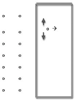
Figure 2: The first photon enters the interferometer. The photon creates the acoustical excitation that in turn generates its cloud of inertons in transverse directions (non-relevant photons are shown before the interferometer).

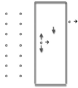
Figure 3: The first photon leaves the interferometer. The following photon just entered the interferometer; the photon creates the appropriate acoustic excitation, which generates a cloud of inertons, and inertons generated by the previous photon are approaching the path of the second photon.

Figure 4: The two photons have already left the interferometer: the second one has experienced a sideways action through the inertons of the first photon. The third photon just enters the interferometer; it experiences sideways action through inertons generated by the two previous photons (through the respective decayed phonons).

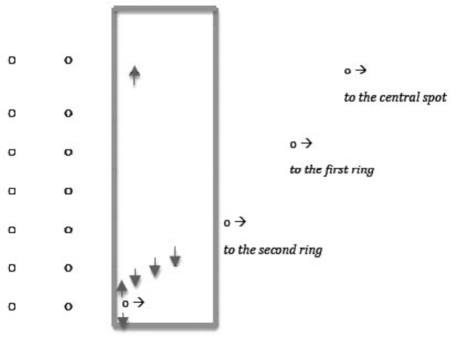
Figure 5: The three photons have already left the interferometer and the fourth photon that has entered the interferometer undergoes sideways action from three flows of inertons generated by the previous photons. The three first photons follow their own trajectories: 1) the first one, which has not been affected by inertons, follows to the centre of the target; 2) the second photon, which was influenced by the first photon (through inertons of the appropriate phonon), is going to form the first ring of the Airy diffraction pattern; 3) the third photon, which underwent the influence of the double flow of inertons (from the two first photons), is deflected to forming the third ring of the Airy pattern, and so on

A similar situation takes place in a foil at the edge of a pinhole. Photons bombard the foil and generate non-equilibrium phonons. The wave vector of phonons ${k}^{\prime}$ practically coincides with the wave vector of incident photons $k$. That is why the phonons decaying in time $\tau$ generate inertons in transverse directions. These inertons intersect the photon flux in the pinhole and are able to affect photons there.

Figure 6: Inertons intersect the pinhole affecting the flow of photons, which results in the formation of the diffraction pattern - the central peak with subsidiary maxima - on the target.

Let us estimate the value of $t$, i.e.

$$t=\frac{{\left({c\pi{\kern 1.0pt}r^{2}/N}\right)^{1/3}}}{{c}},$$ (8)

the time interval when a photon, which follows the previous one, will arrive at the zone of action of inertons generated by the forward photon through the production and decay of a non-equilibrium phonon. Let the radius of the laser beam be $r\approx$ 0.35 cm, then for the three sequential values of photon intensities, used by Panarella [16], $N_{1}\approx 10^{10}$, $N_{2}\approx 10^{8}$ and $N_{3}\approx 10^{4}$ we obtain from expression (8): $t_{1}\approx 1.2\times 10^{-10}$ s, $t_{2}\approx 6\times 10^{-10}$ s and $t_{3}\approx 1.2\times 10^{-8}$ s. The lifetime of non-equilibrium phonons for dielectrics, as mentioned above, varies from 10^-10 s to 10^-8 s [19-22]. Thus if the inequality

$$t\geq\tau$$ (9)

holds, the second photon will arrive to the interferometer at the moment when inertons generated by the first photon will already be absent there. Therefore, the second photon does not experience a transverse action and will continue to follow its path to the central peak on the target. The inequality (9) holds for the case of the lowest intensity of photons, $N_{3}\approx 10^{4}$ photons/sec, namely, $t_{3}>\tau$. Hence the mechanism described is capable to account for Panarella’s experiments in which the diffraction fringe was absent.

The distribution of photons by rings of the diffraction pattern is described in classical optics [24]: the first subsidiary maximum should have an amplitude 0.0175 times the amplitude of the central peak; the second subsidiary maximum has an amplitude 0.0042 times the central amplitude. These results point out that the intensity of transverse inerton flows in the interferometer, which deflects photons from their direct way to the central peak, is not negligible in the case of a comparative high intensity $N$ of the photon flux. What is the reason for such perceptible intensity of inertons?

If the energy of an incident photon is $h\nu$, then the energy of the acoustic excitation produced by the photon is $\hbar\Omega\,\,\,\approx\,\,h\nu{\kern 1.0pt}{\kern 1.0pt}{\kern 1.0pt}\cdot\upsilon_{\rm sound}/c\,\approx\,\,\,10^{-5}{\kern 1.0pt}h\nu$. The energy $\hbar{\kern 1.0pt}\Omega$ is quenched during the time $\tau$ and inertons emitted at the phonon decay carry away an energy no more than $10^{-5}{\kern 1.0pt}h\nu$. This value of energy is not enough to deflect a subsequent photon from the direct line; this would simply fuzzify the width of the central spot from the diameter $d_{{\kern 1.0pt}0}$ to $\left({1+10^{-5}}\right){\kern 1.0pt}\cdot d_{{\kern 1.0pt}0}$.

However, in the interferometer the initial photon produces hundreds or even thousands of acoustic excitations $n_{\rm phon.}$ and hence the intensity of the emitted inerton field will also be a thousand times $10^{-5}{\kern 1.0pt}h\nu$. Then the position of the first ring on the target will be determined by the expression

$$d_{{\kern 1.0pt}1}=l\cdot\tan\frac{{\hbar{\kern 1.0pt}{\kern 1.0pt}\Omega{\kern 1.0pt}{\kern 1.0pt}n_{\rm phon.}}}{{h\nu}}\approx 10^{-5}n_{\rm phon.}\cdot l$$ (10)

where $l$ is the efficient length of the interferometer; the angle of deflection $\phi$ of photons (with the energy $h\nu$) caused by an inerton flow generated by $n_{phon.}$ phonons (with the energy $\hbar\Omega$) is given by the function $\tan\left[{\hbar{\kern 1.0pt}{\kern 1.0pt}\Omega{\kern 1.0pt}{\kern 1.0pt}n_{\rm phon.}/\left({h\nu}\right)}\right]$. In expression (10) we put $\phi<<1$, however, at the same time the flow of inertons is still treated rather intensively, such that $d_{{\kern 1.0pt}1}-d_{{\kern 1.0pt}0}>d_{{\kern 1.0pt}0}$, i.e. the position of the first ring does not overlap with the central spot. Then the second ring is formed by a flow of inertons generated by $2{\kern 1.0pt}n_{\rm phon.}$ phonons (after the first and the second photons), the third ring is formed by inertons generated by $3{\kern 1.0pt}n_{\rm phon.}$ (after the first, second and third photons), etc.

5. Concluding remarks

We have analysed the kinetics of a photon flux in an interferometer. The kinetics show that incident photons producing acoustic excitations (phonons) are responsible also for the emission of inertons. These inertons emerge at the decay of non-equilibrium phonons in a short lifetime $\tau$ and spread in transverse directions to the photon flux. The flow of inertons influences subsequent photons of the photon flux, which deflects some photons from the initial strait line. Following new trajectories, the photons form subsidiary maxima around the central maximum on the target.

It seems the parameter $n_{\rm phon.}$ (the number of phonons needed to generate the transverse flows of inertons for the deflection of photons) allows an experimental verification. Namely, the classical diffraction pattern may appear only when in the interferometer (for instance, a lens) the intensity of photons $N>10^{4}$ photons/sec and the thickness exceeds some critical value. Only starting from a concrete thickness of the lens the number of acoustical excitations will be above the critical value, $n_{\rm phon.}>n_{\rm phon.}^{\left({c}\right)}$, and only at this moment the classical diffraction pattern will be able to emerge following the mechanism described above.

Recently Cardone, Mignany and colleagues [25-27] have revealed anomalous behaviour of photons at crossing photon beam experiments in both the optical and the microwave range. They concluded that the probability wave should be replaced by admitting an interpretation in terms of the Einstein-de Broglie-Bohm “hollow” wave for photons. Those experiments sustain the interpretation of the hollow wave as a deformation of the space-time geometry. These experiments further support the sub-microscopic concept, which has been applied in this study for the explanation of diffraction and non-diffraction of photons. Indeed, the crossing of photon beams has to result in a partial annihilation of colliding photons, such that the surface polarisation is eliminated from these field quasi-particles and only a local volumetric fractal deformation remains. In other words, in the photon-photon collisions the electromagnetic polarisation is compensated and naked inertons appear instead of photons (recall, the photon state is a state of the structured surface of an inerton; the photon state appears on an inerton at the induction of the surface fractality, as shown in Figure 1).

The author thanks greatly J. Perina (Jr.), O. Haderka, M. Dusek and J. Fiurasek, the organisers of the 11th International Conference on Squeezed States and Uncertainty Relations (Olomouc, Czech Republic, 22-26 June 2009) at which this work was delivered.

AFTERWORD

After the publication of this paper I learned about the following papers that dealt with testing of the diffraction phenomenon:

[A1] S. Jeffers, R. Wadlinger and G. Hunter, Low-light-level diffraction experiments: No evidence for anomalous effects, Canad. J. Phys. 6, 91471-1475 (1991).

[A2] S. Jeffers and J. Sloan, A low light level diffraction experiment for anomalies research, J. Scientific Exploration 6, No. 4, 333-352 (1992).

[A3] Yu. P. Dontsov and A. I. Baz, Interference experiments with statistically independent photons, JETF (Journal of Experimental and Theoretical Physics) 52, No. 1, 3-11 (1967); in Russian.

Jeffers et al. [A1, A2] tried to repeat the Panarella’s experiments [16]. Jeffers et al. reported a similar series of Panarella’s low-intensity diffraction experiments (using two different optoelectronic detectors); the lowest intensity of a photon flux reached by Jeffers et al. was the same as was the case of Panarella [16], i.e. 10⁴ photons/sec. However, their results did not substantiate the anomalous effects revealed by Panarella [16] and also Dontsov and Baz [A3].

It should be noted that Jeffers et al. [A1, A2] used the other kind of a hole than the hole used by Panarella; namely, they used a slit, which was bigger in size that a pinhole of Panarella [16]. This means that an area of the screen attacked by photons was also larger in the Jeffers’ experiments. In other words, at Jeffers’ conditions photons, which impacted the screen in the vicinity of the slit, launched non-stationary phonons even at the flux of 10⁴ photons/sec; therefore the decay of excited non-stationary phonons produced inertons in transversal directions. Thus, flows of inertons after the decay of non-stationary phonons were constantly present inside the Jeffers’ slit. Perhaps for the geometry used by Jeffers et al. the intensity of photon flux should be lower than 10⁴ to obtain the result similar to Panarella [16] and Dontsov and Baz [A3].

Dontsov and Baz [A3] were able to achieve an extremely low intensity of statistically independent photons, 200 photons/sec. Their hole had the shape of a slit. They reported that at such a low intensity statistically independent photons passing through a Fabry-Perot interferometer did not form the interference pattern. However, when the intensity of photons was so large that photons emitted by a lamp were in correlated states, the interference pattern was quite distinguishable.

References

- [1] R. N. Boyd, Refutation of Heisenberg uncertainty regarding photons, http://www.rialian.com/rnboyd/heisenburg-refute.htm.
- [2] H. Dehmelt and P. Ekstrom, Proposed g-2/dvz experiment on stored single electron or positron, Bull. Am. Phys. Soc. 18, 727 (1973).
- [3] D. Wineland, P. Ekstrom and H. Dehmelt, Monoelectron oscillator, Phys. Rev. Lett. 31, 1279-1282 (1973).
- [4] R. S. Van Dyck, Jr., P. Ekstrom, and H. Dehmelt, Axial, magnetron, cyclotron and spin-cyclotron beat frequencies measured on single electron almost at rest in free space (Geonium), Nature 262, 776-777 (1976).
- [5] R. S. Van Dyck, Jr., P. B. Schwinberg and H. G. Dehmelt, Electron magnetic moment from geonium spectra: Early experiments and background concepts, Phys. Rev. D 34, 722 - 736 (1986).
- [6] M. Bounias and V. Krasnoholovets, Scanning the structure of ill-known spaces: Part 1. Founding principles about mathematical constitution of space, Kybernetes: The Int. J. Systems and Cybernetics 32, no. 7/8, 945-975 (2003). arXiv.org: physics/0211096.
- [7] M. Bounias and V. Krasnoholovets, Scanning the structure of ill-known spaces: Part 2. Principles of construction of physical space, Kybernetes: The Int. J. Systems and Cybernetics 32, no. 7/8, 976-1004 (2003). arXiv.org: physics/0212004.
- [8] M. Bounias and V. Krasnoholovets, Scanning the structure of ill-known spaces: Part 3. Distribution of topological structures at elementary and cosmic scales, Kybernetes: The Int. J. Systems and Cybernetics 32, no. 7/8, 1005-1020 (2003). arXiv.org: physics/0301049.
- [9] M. Bounias and V. Krasnoholovets, The universe from nothing: A mathematical lattice of empty sets. Int. J. Anticipatory Computing Systems 16, pp. 3-24 (2004), Ed.: D. Dubois. arXiv.org: physics/0309102.
- [10] V. Krasnoholovets, Submicroscopic deterministic quantum mechanics, Int. J. Computing Anticipatory Systems 11, 164-179, 2002. arXiv.org: quant-ph/0109012.
- [11] V. Krasnoholovets, On the theory of the anomalous photoelectric effect stemming from a substructure of matter waves, Indian Journal of Theoretical Physics 49, no. 1, 1-32 (2001). arXiv.org: quant-ph/9906091.
- [12] V. Krasnoholovets, On the notion of the photon, Ann. Fond. L. de Broglie 27, no. 1, 93-100 (2002). arXiv.org: quant-ph/0202170.
- [13] V. Krasnoholovets, On the nature of the electric charge, Hadronic J. Supplement 18, no. 4, pp. 425-456 (2003). arXiv.org: physics/0501132.
- [14] P. S. Epstein and P. Ehrenfest, The quantum theory of the Fraunhofer diffraction, Proc. Natl. Acad. Sci. USA. 10, no. 4, 133-139 (1924).
- [15] P. Ehrenfest and P. S. Epstein, Remarks on the quantum theory of diffraction, Proc. Natl. Acad. Sci. USA 13, no. 6, 400-408 (1927).
- [16] E. Panarella, Nonlinear behavior of light at very low intensities: The “photon clump” model, in Quantum Uncertainties: Recent and future experiments and interpretations. Eds.: W. M. Honig, D. W. Kraft and E. Panarella (Proceedings of NATO, NATO ASI Series, Series B: Physcis 162, New York, and London, USA: Plenum, 1987), pp.105-167.
- [17] C. Kittel, Introduction to solid state physics, Fourth edition (John Wiley and Sons, Inc., New York, London, Sydney, Toronto, 1971), Ch. 5.
- [18] R. Truell, C. Elbaum, and B. B. Chick, Ultrasonic methods in solid state physics (Academy Press, New York, London, 1969), Sections 35-38.
- [19] J. W. Trucker and V. W. Rampton, Microwave ultrasonics in solid state physics (North-Holland Publ.Co., Amsterdam, 1972).
- [20] Sh. Tamura, Spontaneous decay rates of LA phonons in quasi-isotropic solids, Phys. Rev. B 31, No. 4, 2574-2577 (1985).
- [21] W. E. Born, J. L. Patel, and W. L. Schairch. Transport of phonons into diffusive media, Phys. Rev. B 20, No. 12, 5394-5397 (1979).
- [22] Phonon scattering in condensed matter, Eds.: W. Eisenmeger, K. Lasman, and S. Dottinger (Springer, Berlin, 1984).
- [23] V. Krasnoholovets, On variation in mass of entities in condensed media, /it Apeiron /bf 16, no. 4 (2009), in press.
- [24] M. Born and E. Wolf, Principle of optics, 3rd ed. (Pegamon Press, Pxford, 1965), p. 397.
- [25] F. Cardone, R. Mignani, W. Perconti and R. Scrimaglio, The shadow of light: non-Lorentzian behavior of photon systems, Phys. Lett. A 326, 1-13 (2004).
- [26] F. Cardone, R. Mignani, W. Perconti, A. Petrucci and R. Scrimaglio, The shadow of light: further experimental evidences, Int. J. Mod. Phys. B 20, no. 1, 85-98 (2006).
- [27] F. Cardone, R. Mignani, W. Perconti, A. Petrucci and R. Scrimaglio, The shadow of light: Lorentz invariance and complementarity principle in anomalous photon behaviour, Int. J. Mod. Phys. B 20, no. 9 1107-1121 (2006).