Self-propulsion of a catalytically active particle near a planar wall: from reflection to sliding and hovering^†

W. E. Uspal,^ab M. N. Popescu,^abc S. Dietrich,^ab and M. Tasinkevych^∗ab

Received Xth XXXXXXXXXX 20XX, Accepted Xth XXXXXXXXX 20XX
First published on the web Xth XXXXXXXXXX 200X

DOI: 10.1039/b000000x

Micron-sized particles moving through solution in response to self-generated chemical gradients serve as model systems for studying active matter. Their far-reaching potential applications will require the particles to sense and respond to their local environment in a robust manner. The self-generated hydrodynamic and chemical fields, which induce particle motion, probe and are modified by that very environment, including confining boundaries. Focusing on a catalytically active Janus particle as a paradigmatic example, we predict that near a hard planar wall such a particle exhibits several scenarios of motion: reflection from the wall, motion at a steady-state orientation and height above the wall, or motionless, steady “hovering.” Concerning the steady states, the height and the orientation are determined both by the proportion of catalyst coverage and the interactions of the solutes with the different “faces” of the particle. Accordingly, we propose that a desired behavior can be selected by tuning these parameters via a judicious design of the particle surface chemistry.

Autonomous microscopic agents moving through confined, liquid-filled spaces are envisioned as a key component of future lab-on-a-chip and drug delivery systems.¹ Chemically active Janus particles offer a realization of such agents. A Janus “micromotor” works by catalytically activating, over a fraction of its surface, chemical reactions in the surrounding solution. The resulting chemical gradients can drive directed motion through a variety of mechanisms: self-electrophoresis, in which ionic currents drive the motion, of bi-metallic particles;^{‡2, 3} bubble propulsion, in particular for active tubes covered on the inside by a catalyst;⁶ and self-diffusiophoresis, in which the reaction product is electrically neutral, such as for silica or polystyrene spheres covered by platinum.^{7, 8, 9, 10} Recent reviews catalog and detail these and other propulsion mechanisms.^{11, 12, 13} Janus micromotors have been harnessed for applications such as transportation of inert cargo ¹⁰ and environmental remediation.¹⁴

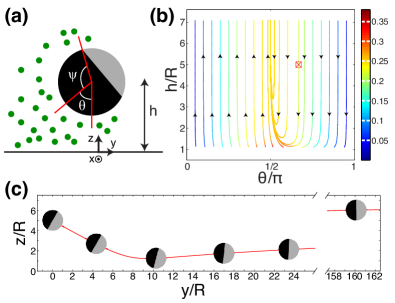
Fig.  1: (a) Schematic diagram of the model system. A sphere of radius $R$ has a surface which is partially catalytic (black) and partially inert (grey). The extent of the catalytic cap is parametrized by $\chi_{0}\equiv-\cos(\psi)$. Green discs indicate a diffusing chemical product. The system is bounded by an inert wall. The height $h$ and the orientation angle $\theta$ specify the configuration of the sphere. (b) Phase plane for half coverage by catalyst ($\chi_{0}=0$) of the Janus particle, where the color encodes $U_{y}/U_{0}$. (c) A typical trajectory of such a Janus particle. The initial configuration is $h_{0}/R=5$ and $\theta_{0}=120^{\circ}$, which is indicated in (b) with the symbol $\boxtimes$.

Recently, several studies have sought to isolate and understand the role of confinement in determining the particle motion. The behavior upon collisions with the confining boundaries was explored in experiments using particles moving in microchannels. Significant motion of Janus particles along the microchannel walls was observed, with subsequent detachment attributed to reorientation of the particle due to thermal noise.^{15, 16} Bi-metallic swimming rods have been observed to orbit around stationary spherical colloids. This behavior has been semi-quantitatively captured via lubrication analysis.¹⁷ In two dimensions, the scenarios of a particle hitting or escaping from a wall are captured by the “Janus active disc” model analyzed in Ref. 18. For certain geometrical configurations and model Janus particles, such as a spherical particle in the center of a spherical cavity ¹⁹ or a dimer translating along the axis of a square tube in a Poiseuille flow,²⁰ the dependence of the particle velocity on the characteristic size of the confinement was obtained via analytical or numerical calculations. For the case of “mechanical swimmers,” modeling micro-organisms which move via shape changes, it was shown theoretically that when motion occurs near a boundary, hydrodynamic interactions can induce a rich dynamical behavior similar to that observed for bacteria^{21, 22, 23, 24} and robotic swimmers.²⁵

Here, we investigate self-diffusiophoresis of a catalytically active spherical Janus particle near a planar boundary. The particle “senses” and responds to the presence of the boundary via the chemical and hydrodynamic fields it creates. Chemically, the particle effectively releases a solute from a catalytic region of its surface. The resulting anisotropic distribution of solute drives a surface flow in a thin layer surrounding the particle, leading to directed motion.^{26, 7, 8, 27, 12} The wall is impenetrable to the solute, modifying the solute number density at the particle surface. Hydrodynamically, the particle creates disturbance flows in the fluid, and these flows are reflected by the no-slip boundary, coupling back to the particle. The issue is to understand how this relation between sensing and response depends on the surface chemistry of the particle.

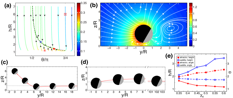
Fig.  2: (a) Phase plane for $\chi_{0}=0.4$. Colors indicate $U_{y}/U_{0}$. There is a dynamical attractor at $h_{eq}/R=1.42$ and $\theta_{eq}=119.9^{\circ}$ (solid red circle). The dashed curve shows the analytically estimated “slow manifold” $U_{z}=0$ (see main text) with a numerically fitted prefactor. (b) Flow field in the laboratory frame (white streamlines) and the solute number density $c/c_{0}$ (colors) associated with the sliding state. (c) A typical trajectory with the initial configuration $h_{0}/R=6$ and $\theta_{0}=3\pi/4$ in the basin of attraction for sliding ($\boxtimes$ in (a)). (d) A trajectory with $h_{0}/R=1.2$ and $\theta_{0}=107.5^{\circ}$ ($\circledast$ in (a)). (e) Variation of the locations of the attractor ($\bullet$) and of the saddle point ($\circ$) with $\chi_{0}$.

Here, we demonstrate that qualitatively distinct dynamics can be evoked by varying certain particle design parameters: (i) the proportion of catalyst coverage, (ii) the repulsive or attractive character of the solute-particle interactions, and (iii) the relative strength of the interactions of the solute with the catalytic and inert particle faces. In particular, for high catalyst coverage and identical repulsive interactions a particle attains a stable state in which it slides along the wall at a fixed height and orientation. Similar dynamics may be obtained for moderate catalyst coverage, but stronger repulsion of the solute from the catalytic than from the inert face. For very high catalyst coverage and repulsive interactions, a particle attains a stable hovering state in which it acts as a stationary micropump. We develop simple quantitative models which shed light on the physical mechanisms sustaining these steady states. We anticipate that these findings can be used in microfluidic devices to create robust and predictable motion of active particles either away from or near walls.

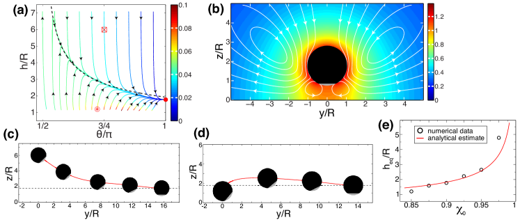
Fig.  3: (a) Phase plane for $\chi_{0}=0.9$. Colors indicate $U_{y}/U_{0}$. There is an attractor at $h_{eq}/R=1.78$ and $\theta_{eq}=180^{\circ}$ (solid red circle). This is a “hovering” state in which the particle remains fixed in space. The dashed curve shows the fitted slow manifold. (b) Flow field (white streamlines) and solute number density $c/c_{0}$ (colors) for the hovering state. These fields are rotationally symmetric about the axis $x=0$, $y=0$. (c) An exemplary trajectory with initial configuration $h_{0}/R=6$ and $\theta_{0}=3\pi/4$ $\boxtimes$ in (a)). (d) The trajectory for $h_{0}/R=1.2$ and $\theta_{0}=130^{\circ}$ ($\circledast$ in (a)). (e) Variation of the height $h_{eq}/R$ of the hovering state with catalyst coverage $\chi_{0}$.

As shown in Fig. 1(a), we consider a spherical particle of radius $R$. The particle is covered by a catalyst over a spherical cap region parametrized by $\chi_{0}=-\cos(\psi)$ (black segment in Fig. 1). The sphere is suspended in a Newtonian liquid solution bounded by a chemically inert planar wall located at $z=0$. The catalytic cap releases a solute which diffuses in the solution. The wall is impenetrable to the solute and there are no other solute-wall interactions. There are effective interactions between the solute and the particle surface. Due to the symmetry of the system and in the absence of thermal fluctuations, the particle moves only in the plane containing the wall normal and the particle’s symmetry axis. Therefore, the cap orientation $\theta$ and the height $h$ of the particle’s center above the wall completely specify the particle configuration. The translational and angular velocities are denoted by $\mathbf{U}$ and $\mathbf{\Omega}$, respectively. We consider the motion of the sphere to be sufficiently slow and the diffusion of the solute to be sufficiently fast such that at each instantaneous $(h,\theta)$ a quasi-steady state of the solute number density $c(\mathbf{r})$ and of the hydrodynamic flow $\mathbf{u}(\mathbf{r})$ is established.

We calculate the self-propulsion velocities $\mathbf{U}$ and $\mathbf{\Omega}$ by employing the classical theory of diffusiophoresis,^{28, 26} which is briefly discussed in the Supplemental Information (SI) along with the associated numerical approach. $\mathbf{U}$ and $\mathbf{\Omega}$ are calculated over a grid of $\theta$ and $h$, which is limited to $h/R\geq 1.1$ for the sake of numerical accuracy and for ensuring the validity of the quasi-steady state approximations discussed above. In order to obtain a full particle trajectory for a certain initial condition $(h_{0},\theta_{0})$, we perform numerical integration by interpolating $\dot{h}=U_{z}$, $\dot{y}=U_{y}$, and $\dot{\theta}=-\Omega_{x}$ from the grid. In the following, the solute number density will be expressed in units of $c_{0}\equiv|\kappa R/D|$ and the velocity in units of $U_{0}\equiv|b\kappa/D|$. $D$ is the diffusion coefficient of the solute and $\kappa$ is the rate of solute production per area at the cap; $b$ is a “surface mobility”; its magnitude and sign reflect the strength and the attractive or repulsive character of the interaction between the solute and the particle surface.²⁶

We first consider a half-covered sphere ($\chi_{0}=0$), and assume uniform repulsion $(b<0)$ of the solute from the particle surface. Our results are summarized in the phase plane of Fig. 1(b). Trajectories starting from initial orientations $\theta_{0}\leq\pi/2$ move away from the wall without a significant change of $\theta$. For $\theta_{0}>\pi/2$ the particle exhibits a richer dynamics. A representative trajectory, with the initial condition given by the symbol $\boxtimes$ in the phase plane [Fig. 1(b)], is shown in Fig. 1(c). The particle moves towards the wall, approximately maintaining its initial orientation of $\theta_{0}=120^{\circ}$ until its scaled height is less than $h/R\simeq 1.5$. In close vicinity of the wall, the particle rotates its catalytic cap towards the wall, e.g. to approximately 100^∘ at $y/R=10$, and further towards $\gtrsim 90^{\circ}$ at $y/R=17$. It escapes from the wall with an asymptotic orientation $\theta\lesssim 90^{\circ}$, which is independent of the initial condition. This behavior – reflection from the wall – is similar to the results derived in Ref. 18 for the motion of a half emitting, half absorbing disc, as well as to the results in Ref. 23 for a spherical “squirmer” near a wall. Note that for larger $\theta_{0}$ the turning point is located closer to the wall; thus, many of the trajectories in this region of the phase space appear to “crash” into the wall (Fig. 1(b)). This is, however, just a numerical artifact meaning that the turning point of the trajectory is below the minimum allowed height.

The mechanism behind the turning point must be driven by the wall through two possible effects: either via the wall induced changes in the solute gradients, affecting the phoretic slip, or via the confinement of the hydrodynamic flow. Smoluchowksi found that solute gradients cannot drive rotation of a particle with uniform $b$,²⁶ hence we anticipate that rotation is dominated by hydrodynamic interaction. The hydrodynamic and chemical effects can be identified and isolated by performing the numerical calculations with properly chosen boundary conditions (see SI). By using this approach, we have been able to confirm that chemical contributions to the rotation of the particle are negligible, except potentially very close to the wall (see SI).

In all cases the rotation of the particle is such as to favor subsequent motion away from the wall, i.e., $\dot{\theta}<0$ for all angles $0<\theta<\pi$. Thus the question arises if states with $\dot{\theta}>0$, i.e., turning towards the wall, or states with $\dot{\theta}=0$ and $U_{z}=0$, which would represent a dynamical fixed point do exist. To address this question, we note that the disturbance flows created by the particle can be described via a superposition of “hydrodynamic singularities,” which are terms in a multipole expansion, centered on the particle, for the flow field surrounding it. The strengths of these singularities determine if and where a curve in the phase plane with $\dot{\theta}=0$ exists.²³ The singularity strengths can be tuned by varying the coverage of the particle by catalyst. For coverages in the range $-1<\chi_{0}<0.35$, the phase planes and trajectories resemble those obtained for half coverage (see Fig. 1(b)). However, at $\chi_{0}=0.35$ a bifurcation occurs: a saddle point and a dynamical attractor emerge. These are illustrated in Fig. 2(a), which shows a phase plane for $\chi_{0}=0.4$. Notably, many trajectories converge, without overlap, to a single curve indicated by the dashed line, which includes both the attractor ($(h_{eq},\theta_{eq})$, solid red circle) and the saddle point (open blue circle). The attractor represents a “sliding” state: the particle maintains a fixed height and orientation as it moves along the wall. The structure of $\mathbf{u}(\mathbf{r})$ and $c(\mathbf{r})$ corresponding to the sliding state is shown in Fig. 2(b).

The curve containing the saddle point and the attractor is a so-called “slow manifold”, characteristic of two-timescale dynamics.²⁹ In the present case, there is a separation of timescales between hydrodynamic interaction driven slow rotation, and rapid self-phoretic vertical motion. The fast variable $h$ quasi-instantaneously adjusts to the slow variable $\theta$, resulting in the convergence of trajectories to a quasi-equilibrium curve $U_{z}=0$ whose functional form can be estimated by a simple argument. We take the manifold to occur where the vertical component of the free space velocity $U_{fs}\cos(\theta)$ is balanced by additional contributions to $U_{z}$ due to the wall. At leading order, the effect of the wall on $c(\mathbf{r})$ can be modeled as an image point source with a spatial gradient $\propto 1/h^{2}$ (see SI). The leading order hydrodynamic contribution to $U_{z}$ also decays as $1/h^{2}$.²³ Thus, we obtain the quasi-equilibrium height $h_{qe}(\theta)\sim(\theta-\pi/2)^{-1/2}$ near $\theta=\pi/2$. With a fitted prefactor, the predicted slow manifold is in a very good agreement with the results of the numerical calculations (see the dashed line in Fig. 2(a) for $\chi_{0}=0.4$).

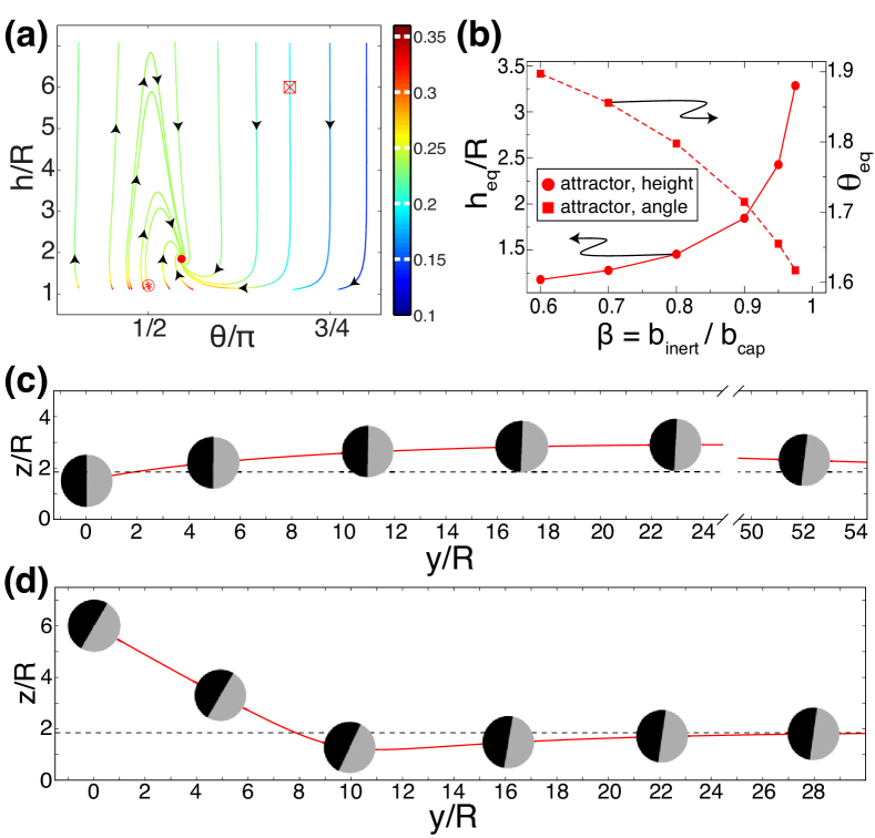
Fig.  4: (a) Phase plane for half coverage ($\chi_{0}=0$) and unequal surface mobilities: $\beta=b_{inert}/b_{cap}=0.9$. There is an attractor at $h_{eq}/R=1.85$ and $\theta_{eq}=98.2^{\circ}$ ($\bullet$). Colors indicate $U_{y}/U_{0}$, where $U_{0}\equiv|b_{cap}\kappa/D|$. (b) Variation of the attractor location with $\beta$ for half coverage. (c) Trajectory with initial configuration $h_{0}/R=1.2$ and $\theta_{0}=\pi/2$ ($\circledast$ in (a)). (d) Trajectory with $h_{0}/R=6$ and $\theta_{0}=125^{\circ}$ ($\boxtimes$ in (a)). This is the same initial configuration as in Fig. 1(c).

Upon increasing $\chi_{0}$ further, we find that $\theta_{eq}$ increases and $h_{eq}$ decreases (see Fig. 2(e)). For $\chi_{0}>0.6$, the dynamical attractor migrates below $h/R=1.1$. However, at $\chi_{0}=0.85$, an attractor emerges at $\theta=\pi$. For this attractor, $U_{y}=0$: the particle “hovers” in space and acts as a stationary micropump (see Fig. 3(b)). As shown in Fig. 3(a), the basin of attraction for “hovering” at $\chi_{0}=0.9$ encompasses nearly half of the phase space. The mechanism of the hovering state is understood by balancing the free space velocity with the wall-induced contributions to $U_{z}$, dominated by the leading order solute number density term (the image point source), which gives $h_{eq}/R=[3(1-\chi_{0})]^{-1/2}$ (see SI for details). This expression, for most values of $\chi_{0}$, is in good agreement with the numerical results (see Fig. 3(e)).

So far only the case of uniform surface mobility $b<0$ was considered. Here we briefly outline the main effects induced by allowing the ratio $\beta\equiv b_{inert}/b_{cap}$ of the surface mobilities across the inert and catalytic regions to take values different than one. Since $\beta\neq 1$ introduces an additional mechanism for rotating the particle (see SI), we expect that by adjusting $\beta$ sliding states can be induced also at the experimentally relevant case of half coverage $\chi_{0}=0$. For $\beta>1$ we obtain the reflection only with no dynamical attractor. For values $\beta<1$, however, sliding states occur with $h_{eq},\theta_{eq}$ depending on $\beta$ (see Fig. 4). Physically, this occurs because of the stronger product repulsion from the cap than from the inert side. Therefore it becomes possible for the wall-induced chemical gradient to drive a rotation of the cap away from the wall.

Briefly, we consider the effect of thermal noise, which so far has been neglected. Numerically, we can estimate the “stiffness” of a steady state by computing the eigenvalues of the Jacobian at the fixed point $(h^{*},\theta^{*})$. For the sliding state with $\chi_{0}=0.4$, we obtain eigenvalues $\lambda_{1}R/U_{0}=-0.011$ and $\lambda_{2}R/U_{0}=-0.145$, reflecting the separation of timescales discussed previously. For the hovering state with $\chi_{0}=0.9$, we obtain eigenvalues $\lambda_{1}R/U_{0}=-0.014$ and $\lambda_{2}R/U_{0}=-0.059$. Considering a typical catalytic Janus colloid of $R=2.5\>\mu m$, half covered by catalyst, and moving, if unconfined, with speed $U_{fs}=5\>\mu m/s$, one has $U_{0}=20\>\mu m/s$ (for half coverage, $U_{fs}=U_{0}/4$).²⁷ Therefore, for both steady states we obtain $\tau_{1}\approx 10\>s$ as the longest timescale for self-trapping via near-surface swimming. In comparison, for the same colloid the timescale $\tau_{r}$ for reorienting via rotational diffusion is $\tau_{r}=D_{r}^{-1}=8\pi\mu R^{3}/k_{B}T$. In water at room temperature this renders as $\tau_{r}\approx 95\>s$. Similarly, the characteristic timescale for translational diffusion (i.e., a perturbation along vertical direction) is $\tau_{t}=R^{2}/D=6\pi\mu R^{3}/k_{B}T$, leading to $\tau_{t}\approx 70\>s$. Therefore, for a typical catalytic Janus particle we expect the sliding and hovering states to be robust against thermal noise. For particles with half coverage, we anticipate that both deterministic swimming and rotational diffusion promote the experimentally observed scenario of transient near-surface swimming followed by escape. ^{15, 16} A study including both effects would be a natural extension of this work.

Finally, we comment on the case of attractive ($b>0$) solute-particle interactions. It is easy to see that in this case the sole change in the equations describing the self-propulsion is that the phoretic slip changes sign. Therefore, the phase planes, trajectories, and flow structures can be inferred from the ones corresponding to $b<0$ by simply reversing the directions of the arrows. In this case the sliding and hovering attractors will turn into repellers, saddle points stay the same, and a particle always either “crashes” into the wall or moves away from it, in contrast to the complex behavior observed in the case of repulsive interactions.

To conclude, a catalytically active Janus particle moving near a wall reveals a very rich behavior, including reflection, steady sliding, and hovering. Although we have focused on self-diffusiophoresis, we expect, following the line of reasoning and argumentation presented in Ref. 8, that our results could be relevant for more complex mechanisms of propulsion, like self-thermophoresis^{30, 31} or self-electrophoresis.^{3, 17} The sliding states could provide a starting point to establish a stable and predictable motion of swimmers in microdevices. The sliding mechanism outlined here could account for the experimental observations reported in Ref. 4, namely an accumulation of catalytically active particles near both the upper and the lower surfaces in capillaries. Hovering particles create recirculating regions of flow, and could be used to mix fluid or to trap other particles. Our findings highlight the significant role played by the wall-induced chemical gradients: due to coupling back to the particle motion via changing the phoretic slip on the particle surface (neglected in previous studies of active particles near interfaces), they induce distinct types of motion of the particle. Finally, we have shown how qualitative and quantitative changes in the behavior can be achieved in a controlled way by adequately tuning experimentally accessible design parameters of Janus particles, such as the extent of catalytic coverage $\chi_{0}$ and the spatial variation of the surface mobility $b$. A detailed study, which considers more general boundary conditions at the wall (such as phoretic slip, or a “porous” wall), as well as general values of the parameters $\beta$ and $\chi_{0}$, is currently in progess.

The authors wish to thank C. Pozrikidis for making freely available the BEMLIB library, which was used for the present numerical computations.³² W.E.U, M.T., and M.N.P. acknowledge financial support from the DFG, grant No. TA 959/1-1.

See pages 1-last of self_propelled_SI_SM_revised_final_accepted.pdf

References

- Patra et al. 2013 D. Patra, S. Sengupta, W. Duan, H. Zhang, R. Pavlick and A. Sen, Nanoscale, 2013, 5, 1273–1283.
- Paxton et al. 2004 W. F. Paxton, K. C. Kistler, C. C. Olmeda, A. Sen, S. K. St. Angelo, Y. Y. Cao, T. E. Mallouk, P. E. Lammert and V. H. Crespi, J. Am. Chem. Soc., 2004, 126, 13424–13431.
- Paxton et al. 2006 W. Paxton, P. Baker, T. Kline, Y. Wang, T. Mallouk and A. Sen, Angew. Chem. Int. Ed., 2006, 128, 14881–14888.
- Brown and Poon 2014 A. Brown and W. Poon, Soft Matter, 2014, 10, 4016–4027.
- Ebbens et al. 2014 S. Ebbens, D. A. Gregory, G. Dunderdale, J. R. Howse, Y. Ibrahim, T. B. Liverpool and R. Golestanian, EPL, 2014, 106, 58003.
- Gao et al. 2012 W. Gao, A. Pei and J. Wang, ACS Nano, 2012, 6, 8432–8438.
- Golestanian et al. 2005 R. Golestanian, T. B. Liverpool and A. Ajdari, Phys. Rev. Lett., 2005, 94, 220801.
- Golestanian et al. 2007 R. Golestanian, T. B. Liverpool and A. Ajdari, New J. Phys., 2007, 9, 126.
- Howse et al. 2007 J. Howse, R. Jones, A.J.Ryan, T. Gough, R. Vafabakhsh and R. Golestanian, Phys. Rev. Lett., 2007, 99, 048102.
- Baraban et al. 2012 L. Baraban, M. Tasinkevych, M. N. Popescu, S. Sanchez, S. Dietrich and O. G. Schmidt, Soft Matter, 2012, 8, 48–52.
- Ebbens and Howse 2010 S. J. Ebbens and J. R. Howse, Soft Matter, 2010, 6, 726–738.
- Poon 2013 W. C. K. Poon, Proceedings of the International School of Physics “Enrico Fermi”, Course CLXXXIV “Physics of Complex Colloids”, Amsterdam, 2013, p. 317.
- Wang et al. 2013 W. Wang, W. Duan, S. Ahmed, T. E. Mallouk and A. Sen, Nano Today, 2013, 8, 531–554.
- Gao et al. 2013 W. Gao, X. Feng, A. Pei, Y. Gu, J. Li and J. Wang, Nanoscale, 2013, 5, 4696–4700.
- Volpe et al. 2011 G. Volpe, I. Buttinoni, D. Vogt, H.-J. Kümmerer and C. Bechinger, Soft Matter, 2011, 7, 8810–8815.
- Kreuter et al. 2013 C. Kreuter, U. Siems, P. Nielaba, P. Leiderer and A. Erbe, Eur. Phys. J. Special Topics, 2013, 222, 2923–2939.
- Takagi et al. 2014 D. Takagi, J. Palacci, A. B. Braunschweig, M. J. Shelley and J. Zhang, Soft Matter, 2014, 10, 1784–1789.
- Crowdy 2013 D. G. Crowdy, J. Fluid Mech., 2013, 735, 473–498.
- Popescu et al. 2009 M. N. Popescu, S. Dietrich and G. Oshanin, J. Chem. Phys., 2009, 130, 194702.
- Tao and Kapral 2010 Y.-G. Tao and R. Kapral, Soft Matter, 2010, 6, 756–761.
- Lauga et al. 2006 E. Lauga, W. D. Luzio, G. M. Whitesides and H. Stone, Biophys. J., 2006, 90, 400–412.
- Berke et al. 2008 A. Berke, L. Turner, H. Berg and E. Lauga, Phys. Rev. Lett., 2008, 101, 038102.
- Spangolie and Lauga 2012 S. Spangolie and E. Lauga, J. Fluid Mech., 2012, 700, 105–147.
- Ishimoto and Gaffney 2013 K. Ishimoto and E. A. Gaffney, Phys. Rev. E, 2013, 88, 062702.
- Zhang et al. 2010 S. Zhang, Y. Or and R. M. Murray, Proc. Am. Control Conf., 2010, pp. 4205–4210.
- Anderson 1989 J. L. Anderson, Ann. Rev. Fluid Mech., 1989, 21, 61–99.
- Popescu et al. 2010 M. N. Popescu, S. Dietrich, M. Tasinkevych and J. Ralston, Eur. Phys. J. E, 2010, 31, 351–367.
- Derjaguin et al. 1947 B. V. Derjaguin, G. P. Sidorenkov, E. A. Zubashchenkov and E. V. Kiseleva, Kolloidn. Zh., 1947, 9, 335.
- Murdock 1999 J. A. Murdock, Perturbations: Theory and Methods, SIAM, Philadelphia, PA, 1999.
- Jiang et al. 2010 H.-R. Jiang, N. Yoshinaga and M. Sano, Phys. Rev. Lett., 2010, 105, 268302.
- Yang et al. 2014 M. Yang, A. Wysocki and M. Ripoll, Soft Matter, 2014, 10, 6208–6218.
- Pozrikidis 2002 C. Pozrikidis, A Practical Guide to Boundary Element Methods with the Software Library BEMLIB, CRC Press, Boca Raton, 2002.