Controlling quantum-dot light absorption and emission by a surface-plasmon field

Abstract

The possibility for controlling the probe-field optical gain and absorption switching and photon conversion by a surface-plasmon-polariton near field is explored for a quantum dot above the surface of a metal. In contrast to the linear response in the weak-coupling regime, the calculated spectra show an induced optical gain and a triply-split spontaneous emission peak resulting from the interference between the surface-plasmon field and the probe or self-emitted light field in such a strongly-coupled nonlinear system. Our result on the control of the mediated photon-photon interaction, very similar to the ‘gate’ control in an optical transistor, may be experimentally observable and applied to ultra-fast intrachip/interchip optical interconnects, improvement in the performance of fiber-optic communication networks and developments of optical digital computers and quantum communications.

I Introduction

It is well known that photons inherently do not interact with each other. In classical electrodynamics, the Maxwell equations are linear and cannot describe any photon-photon interaction. However, effective photon-photon coupling could exist in a mediated way, e.g. through their direct interactions with matter. Very recently, an experiment lukin , which involves firing pairs of photons through an ultra-cold atomic gas, was reported to provide the evidence for an attractive interaction between the photons to form the so called ‘molecules’ of light. In general, if the interaction between photons and matter is strong, the optical response of matter will become nonlinear and the resulting bandedge optical nonlinearities r7 will enable an effective photon-photon interaction. sci An optical transistor otrans could be built based on this basic idea, where ‘gate’ photons control the intensity of a ‘source’ light beam. Optical transistors could be applied to speed up and improve the performance of fiber-optic communication networks. Here, all-optical digital signal processing and routing is fulfilled by arranging optical transistors in photonic integrated circuits and the signal loss during the propagation could be compensated by inserting new types of optical amplifiers. Moreover, optical transistors are expected to play an important role in the developments of an optical digital computer or quantum-encrypted communication.

Most previous research on optical properties of materials, including optical absorption, inelastic light scattering and spontaneous emission, used a weak probe field as a perturbation to the studied system. book In this weak-coupling regime, the optical response of electrons depends only on the material characteristics, linear and therefore, no photon-photon interaction is expected. However, the strong-coupling regime could be reached with help from microcavities and the experimental effort on searching for polariton condensation (resulting from strong light-electron interaction) in semiconductors continues to produce results. polar1 ; polar2 ; polar3 The general review of exciton-polariton condensation can be found from Ref. [rmp, ]. The successful demonstration of room-temperature polariton lasing without population inversion in semiconductor microcavities using both optical pumping pump1 ; pump2 and electrical injection injec1 ; injec2 have made it possible for ultra-low lasing thresholds and very-small emitter sizes comparable to the emitted wavelength. Semiconductor exciton-polariton nanolasers could advance intrachip and interchip optical interconnects by integrating them into semiconductor-based photonic chips, and they might also have applications in medical devices and treatments, such as spatially selective illumination of individual neuron cells to locally control neuron firing activities in optogenetics and neuroscience and near-field high-resolution imaging beyond the optical diffraction limit as well.

Theoretically, a big hurdle also exists for studying photon-photon interactions in the strong-coupling regime mainly due to intractable numerical computation for systems with very strong nonlinearity. The obstacle of nonlinearity in such a system means that any perturbative theories, e.g. using bare electron states or linear response theory, book become inadequate for describing both field and electron dynamics in this system. The presence of an induced polarization, regarded as a source term to the Maxwell equations, r6 ; apl from photo-excited electrons makes it impossible for us to solve the field equations by simply using finite-element analysis fem or finite-difference-time-domain methods fdtd . Although the semiconductor-Bloch equations koch1 and density-matrix equations book ; r9 , derived from many-body theory, are able to accurately capture the nonlinear optical response of electrons, the inclusion of pair scattering effects on both energy relaxation and optical dephasing precludes an analytical approach for seeking solution of these equations. As a result, there exists only very few theoretical studies koch , which heavily depend on computer simulation, that focus on simplified one-dimensional strongly-coupled microcavity systems, in contrast to the three-dimensional structure and self-consistent approach presented in this paper.

Physically, not only the high-quality microcavities Scherer but also the intense surface-plasmon near fields sp1 ; sp2 could be employed for reaching the strong-coupling goal in semiconductors. In this paper we solve the self-consistent equations for strongly-coupled electromagnetic-field dynamics and electron quantum kinetics in a quantum dot above the surface of a thick metallic film, which has not been fully explored so far from either a theoretical or experimental point of view. This is done based on finding an analytical solution to Green’s function aam1 ; aam2 for a quantum dot coupled to a semi-infinite metallic material system, which makes it easy to calculate the effect of the induced polarization field as a source term to the Maxwell equations. In our formalism, the strong light-electron interaction is reflected in the photon-dressed electronic states with a Rabi gap and in the feedback from the induced optical polarization of dressed electrons to the incident light. The formalism derived in this paper goes beyond the weak-coupling limit and deals with a much more realistic structure in the strong-coupling limit for the development of a surface-plasmon polariton laser with a very low threshold pumping. Our results clearly demonstrate the ability to control probe-field optical gain and absorption switching and photon conversion by a surface-plasmon field with temperature-driven frequency detuning in such a nonlinear system led by dressed electron states, very similar to the ‘gate’ control in an optical transistor. These conclusions should be experimentally observable spie ; ol . On the other hand, our numerical results also provide an example for demonstrating the so-called quantum plasmonics, natphys where the nature of surface-plasmon polaritons and the nature of quantum-confined electrons are hybridized through near-field coupling.

In Sec. II, we will introduce our physics model and derive self-consistent equations for determining the coupled scattering dynamics of a surface-plasmon field and the quantum kinetics of electrons in quantum dots. Section III is devoted to a full discussion of our numerical results, including scattering and optical absorption of surface-plasmon-polariton field by quantum dots, spontaneous emission and nonlinear optical response of dressed electron states. Some concluding remarks are given in Sec. IV.

II Model and Theory

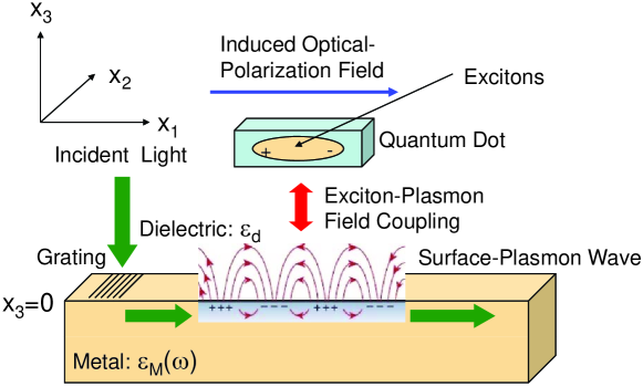
Figure 1: (Color online) Schematic illustration for a semi-infinite metal and a quantum dot above its surface at $x_{3}=0$. Here, the surface-plasmon polariton (SPP) is locally excited by incident light with the help of a surface grating. The propagating SPP field further excites e-h pairs (plasmas) in the adjacent quantum dot. As a result, the optical-polarization field of the photo-excited e-h plasma is strongly coupled to the propagating SPP field to form split plasma-SPP modes with an anticrossing gap. Also, a probe-field is used for studying the photon dressing effect.

Our model system, as shown in Fig. 1, consists of a semi-infinite metallic materialwith a semiconductor quantum dot above its surface. A surface-plasmon-polariton (SPP) field is locally excited through a surface grating by normally-incident light. This propagating SPP field further excites an interband electron-hole (e-h) plasma in the quantum dot. The induced optical-polarization field of the photo-excited e-h plasma is strongly coupled to the SPP field to produce split degenerate e-h plasma and SPP modes with an anticrossing gap. Part of the brief description for our self-consistent formalism was reported earlier. apl In order to let readers follow up easily with the details of our model and formalism, we present here the full derivation of the Maxwell-Bloch numerical approach for an SPP field coupled to a photo-excited e-h plasma in the quantum dot.

II.1 General Formalism

The Maxwell’s equation for a semi-infinite non-magnetic medium in position-frequency space can be written as aam1

$$\mbox{\boldmath$\nabla$$\times$\boldmath$\nabla$$\times$\boldmath$E$}({\bf r};\,\omega)-\epsilon_{\rm b}(x_{3};\,\omega)\,\frac{\omega^{2}}{c^{2}}\,\mbox{\boldmath$E$}({\bf r};\,\omega)=\frac{\omega^{2}}{\epsilon_{0}c^{2}}\,\mbox{\boldmath${\cal P}$}^{\rm loc}({\bf r};\,\omega)\ ,$$ (1)

where $\mbox{\boldmath$E$}({\bf r};\,\omega)$ is the electric component of an electromagnetic field, $\displaystyle{\mbox{\boldmath$H$}({\bf r};\,\omega)=-\left(\frac{i}{\omega\mu_{0}}\right)\mbox{\boldmath$\nabla$$\times$\boldmath$E$}({\bf r};\,\omega)}$ is the magnetic component of the electromagnetic field, ${\bf r}=(x_{1},x_{2},x_{3})$ is a three-dimensional position vector, $\omega$ is the angular frequency of the incident light, $\epsilon_{0}$, $\mu_{0}$ and $c$ are the permittivity, permeability and speed of light in vacuum, $\mbox{\boldmath${\cal P}$}^{\rm loc}({\bf r};\,\omega)$ is an off-surface local polarization field generated by optical transitions of electrons in a quantum dot, and the position-dependent dielectric function is

$$\epsilon_{\rm b}(x_{3};\,\omega)=\left\{\begin{array}[]{ll}\epsilon_{\rm d}\ ,&\mbox{for $x_{3}>0$}\\ \epsilon_{\rm M}(\omega)\ ,&\mbox{for $x_{3}<0$}\end{array}\right.\ .$$ (2)

Here, $\epsilon_{\rm d}$ is for the semi-infinite dielectric material in the region $x_{3}>0$, while $\epsilon_{\rm M}(\omega)$ represents the semi-infinite metallic material in the region $x_{3}<0$. For the Maxwell’s equation in Eq. (1), we introduce the Green’s function ${\cal G}_{\mu\nu}({\bf r},{\bf r}^{\prime};\,\omega)$ satisfying the following equation

$$\sum\limits_{\mu}\left[\epsilon_{\rm b}(x_{3};\,\omega)\,\frac{\omega^{2}}{c^{2}}\,\delta_{\lambda\mu}-\frac{\partial^{2}}{\partial x_{\lambda}\partial x_{\mu}}+\delta_{\lambda\mu}\,\nabla_{\bf r}^{2}\right]{\cal G}_{\mu\nu}({\bf r},{\bf r}^{\prime};\,\omega)=\delta_{\lambda\nu}\,\delta({\bf r}-{\bf r}^{\prime})\ ,$$ (3)

where $\displaystyle{\nabla_{\bf r}^{2}=\sum\limits_{\mu}\,\frac{\partial^{2}}{\partial x^{2}_{\mu}}}$ is the Laplace operator, $\delta_{\lambda\mu}$ represents the Kronecker delta, and the indices $\lambda,\,\mu=1,\,2,\,3$ indicate three spatial directions. Using the Green’s function defined in Eq. (3), we can convert the Maxwell’s equation in Eq. (1) into a three-dimensional integral equation

$$E_{\mu}({\bf r};\,\omega)=E^{(0)}_{\mu}({\bf r};\,\omega)-\frac{\omega^{2}}{\epsilon_{0}c^{2}}\sum\limits_{\nu}\int d^{3}{\bf r}^{\prime}\,{\cal G}_{\mu\nu}({\bf r},{\bf r}^{\prime};\,\omega)\,{\cal P}_{\nu}^{\rm loc}({\bf r}^{\prime};\,\omega)\ ,$$ (4)

where $E^{(0)}_{\mu}({\bf r};\,\omega)$ is a solution of the corresponding homogeneous equation

$$\sum\limits_{\nu}\left[\epsilon_{\rm b}(x_{3};\,\omega)\,\frac{\omega^{2}}{c^{2}}\,\delta_{\mu\nu}-\frac{\partial^{2}}{\partial x_{\mu}\partial x_{\nu}}+\delta_{\mu\nu}\,\nabla^{2}_{\bf r}\right]E^{(0)}_{\nu}({\bf r};\,\omega)=0\ ,$$ (5)

and the source term ${\cal P}_{\nu}^{\rm loc}({\bf r}^{\prime};\,\omega)$ generally depends on the electric field in a nonlinear way and can be determined by the Bloch equation. r6 ; r7

II.2 Solving Green’s Function

For a semi-infinite medium, the Green’s function can be formally expressed by its Fourier transform

$${\cal G}_{\mu\nu}({\bf r},{\bf r}^{\prime};\,\omega)=\int\frac{d^{2}{\bf k}_{\|}}{(2\pi)^{2}}\,e^{i{\bf k}_{\|}\cdot({\bf r}_{\|}-{\bf r}^{\prime}_{\|})}\,g_{\mu\nu}({\bf k}_{\|},\omega|x_{3},x_{3}^{\prime})\ ,$$ (6)

where we have introduced the notations for the two-dimensional vectors ${\bf r}_{\|}=(x_{1},x_{2})$ and ${\bf k}_{\|}=(k_{1},k_{2})$. Substituting Eq. (6) into Eq. (3), we obtain

$$\left[\begin{array}[]{ccc}\displaystyle{\epsilon_{b}\,\frac{\omega^{2}}{c^{2}}-k_{2}^{2}+\frac{d^{2}}{dx_{3}^{2}}}&k_{1}k_{2}&\displaystyle{-ik_{1}\frac{d}{dx_{3}}}\\ k_{1}k_{2}&\displaystyle{\epsilon_{b}\,\frac{\omega^{2}}{c^{2}}-k_{1}^{2}+\frac{d^{2}}{dx_{3}^{2}}}&\displaystyle{-ik_{2}\frac{d}{dx_{3}}}\\ \displaystyle{-ik_{1}\frac{d}{dx_{3}}}&\displaystyle{-ik_{2}\frac{d}{dx_{3}}}&\displaystyle{\epsilon_{b}\,\frac{\omega^{2}}{c^{2}}-k_{\|}^{2}}\end{array}\right]\,\left[\begin{array}[]{ccc}g_{11}&g_{12}&g_{13}\\ g_{21}&g_{22}&g_{23}\\ g_{31}&g_{32}&g_{33}\end{array}\right]=\delta(x_{3}-x_{3}^{\prime})\,\left[\begin{array}[]{ccc}1&0&0\\ 0&1&0\\ 0&0&1\end{array}\right]\ .$$ (7)

After a rotational transformation aam1 is performed in ${\bf k}_{\|}$-space, i.e.,

$$f_{\mu\nu}(k_{\|},\omega|x_{3},x_{3}^{\prime})=\sum\limits_{\mu^{\prime},\nu^{\prime}}\,{\cal S}_{\mu\mu^{\prime}}({\bf k}_{\|})\,{\cal S}_{\nu\nu^{\prime}}({\bf k}_{\|})\,g_{\mu^{\prime}\nu^{\prime}}({\bf k}_{\|},\omega|x_{3},x_{3}^{\prime})\ ,$$ (8)

where the rotational matrix is selected as

$${\cal S}({\bf k}_{\|})=\frac{1}{k_{\|}}\,\left[\begin{array}[]{ccc}k_{1}&k_{2}&0\\ -k_{2}&k_{1}&0\\ 0&0&k_{\|}\end{array}\right]\ ,$$ (9)

we acquire an equivalent version of Eq. (7)

$$\left[\begin{array}[]{ccc}\displaystyle{\epsilon_{b}\,\frac{\omega^{2}}{c^{2}}+\frac{d^{2}}{dx_{3}^{2}}}&0&\displaystyle{-ik_{\|}\frac{d}{dx_{3}}}\\ 0&\displaystyle{\epsilon_{b}\,\frac{\omega^{2}}{c^{2}}-k_{\|}^{2}+\frac{d^{2}}{dx_{3}^{2}}}&0\\ \displaystyle{-ik_{\|}\frac{d}{dx_{3}}}&0&\displaystyle{\epsilon_{b}\,\frac{\omega^{2}}{c^{2}}-k_{\|}^{2}}\end{array}\right]\,\left[\begin{array}[]{ccc}f_{11}&f_{12}&f_{13}\\ f_{21}&f_{22}&f_{23}\\ f_{31}&f_{32}&f_{33}\end{array}\right]=\delta(x_{3}-x_{3}^{\prime})\,\left[\begin{array}[]{ccc}1&0&0\\ 0&1&0\\ 0&0&1\end{array}\right]\ .$$ (10)

To get the solution of Eq. (10), we need to employ both the finite-value boundary condition at $x_{3}^{\prime}=\pm\infty$ and the continuity boundary condition at the $x_{3}=0$ interface. This leads to the following five non-zero $f_{\mu\nu}(k_{\|},\omega|x_{3},x_{3}^{\prime})$ elements aam1 ; aam2

$$f_{22}(k_{\|},\omega|x_{3},x_{3}^{\prime})$$ (18)

$$= \left\{\begin{array}[]{llll}\displaystyle{-\left(\frac{i}{2p}\right)\frac{2p}{p_{\rm d}+p}\ e^{ip_{\rm d}x_{3}-ipx_{3}^{\prime}}}\ ,&x_{3}>0\ ,\,x_{3}^{\prime}<0\\ \\ \displaystyle{-\left(\frac{i}{2p}\right)\left[e^{ip|x_{3}-x_{3}^{\prime}|}-\frac{p_{\rm d}-p}{p_{\rm d}+p}\ e^{-ip(x_{3}+x_{3}^{\prime})}\right]}\ ,&x_{3}<0\ ,\,x_{3}^{\prime}<0\\ \\ \displaystyle{-\left(\frac{i}{2p_{\rm d}}\right)\left[e^{ip_{\rm d}|x_{3}-x_{3}^{\prime}|}+\frac{p_{\rm d}-p}{p_{\rm d}+p}\ e^{ip_{\rm d}(x_{3}+x_{3}^{\prime})}\right]}\ ,&x_{3}>0\ ,\,x_{3}^{\prime}>0\\ \\ \displaystyle{-\left(\frac{i}{2p_{\rm d}}\right)\frac{2p_{\rm d}}{p_{\rm d}+p}\ e^{-ip(x_{3}-x_{3}^{\prime})}}\ ,&x_{3}<0\ ,\,x_{3}^{\prime}>0\end{array}\right.\ ,\ \$$

$$f_{13}(k_{\|},\omega|x_{3},x_{3}^{\prime})$$ (26)

$$= \left\{\begin{array}[]{llll}\displaystyle{\frac{ik_{\|}c^{2}}{2\epsilon_{\rm M}(\omega)\omega^{2}}\left[\frac{2\epsilon_{\rm M}(\omega)p_{\rm d}}{\epsilon_{\rm M}(\omega)p_{\rm d}+\epsilon_{\rm d}\,p}\right]\,e^{ip_{\rm d}x_{3}-ipx_{3}^{\prime}}}\ ,&x_{3}>0\ ,\,x_{3}^{\prime}<0\\ \\ \displaystyle{\frac{ik_{\|}c^{2}}{2\epsilon_{\rm M}(\omega)\omega^{2}}\left[e^{ip|x_{3}-x_{3}^{\prime}|}\,{\rm sgn}(x_{3}-x_{3}^{\prime})+\frac{\epsilon_{\rm M}(\omega)p_{\rm d}-\epsilon_{\rm d}\,p}{\epsilon_{\rm M}(\omega)p_{\rm d}+\epsilon_{\rm d}\,p}\ e^{-ip(x_{3}+x_{3}^{\prime})}\right]}\ ,&x_{3}<0\ ,\,x_{3}^{\prime}<0\\ \\ \displaystyle{\frac{ik_{\|}c^{2}}{2\epsilon_{\rm d}\,\omega^{2}}\left[e^{ip_{\rm d}|x_{3}-x_{3}^{\prime}|}\,{\rm sgn}(x_{3}-x_{3}^{\prime})+\frac{\epsilon_{\rm M}(\omega)p_{\rm d}-\epsilon_{\rm d}\,p}{\epsilon_{\rm M}(\omega)p_{\rm d}+\epsilon_{\rm d}\,p}\ e^{ip_{\rm d}(x_{3}+x_{3}^{\prime})}\right]}\ ,&x_{3}>0\ ,\,x_{3}^{\prime}>0\\ \\ \displaystyle{-\frac{ik_{\|}c^{2}}{2\epsilon_{\rm d}\,\omega^{2}}\left[\frac{2\epsilon_{\rm d}\,p}{\epsilon_{\rm M}(\omega)p_{\rm d}+\epsilon_{\rm d}\,p}\right]\,e^{-ipx_{3}+ip_{\rm d}x_{3}^{\prime}}}\ ,&x_{3}<0\ ,\,x_{3}^{\prime}>0\end{array}\right.$$

$$f_{33}(k_{\|},\omega|x_{3},x_{3}^{\prime})$$ (34)

$$= \left\{\begin{array}[]{llll}\displaystyle{-\frac{ik^{2}_{\|}c^{2}}{\omega^{2}}\left[\frac{1}{\epsilon_{\rm M}(\omega)p_{\rm d}+\epsilon_{\rm d}\,p}\right]\,e^{ip_{\rm d}x_{3}-ipx_{3}^{\prime}}}\ ,&x_{3}>0\ ,\,x_{3}^{\prime}<0\\ \\ \displaystyle{\frac{c^{2}}{\epsilon_{\rm M}(\omega)\omega^{2}}\,\delta(x_{3}-x_{3}^{\prime})-\frac{ik^{2}_{\|}c^{2}}{2p\,\epsilon_{\rm M}(\omega)\omega^{2}}\left[e^{ip|x_{3}-x_{3}^{\prime}|}-\frac{\epsilon_{\rm M}(\omega)p_{\rm d}-\epsilon_{\rm d}\,p}{\epsilon_{\rm M}(\omega)p_{\rm d}+\epsilon_{\rm d}\,p}\ e^{-ip(x_{3}+x_{3}^{\prime})}\right]}\ ,&x_{3}<0\ ,\,x_{3}^{\prime}<0\\ \\ \displaystyle{\frac{c^{2}}{\epsilon_{\rm d}\,\omega^{2}}\,\delta(x_{3}-x_{3}^{\prime})-\frac{ik_{\|}^{2}c^{2}}{2p_{\rm d}\epsilon_{\rm d}\,\omega^{2}}\left[e^{ip_{\rm d}|x_{3}-x_{3}^{\prime}|}+\frac{\epsilon_{\rm M}(\omega)p_{\rm d}-\epsilon_{\rm d}\,p}{\epsilon_{\rm M}(\omega)p_{\rm d}+\epsilon_{\rm d}\,p}\ e^{ip_{\rm d}(x_{3}+x_{3}^{\prime})}\right]}\ ,&x_{3}>0\ ,\,x_{3}^{\prime}>0\\ \\ \displaystyle{-\frac{ik^{2}_{\|}c^{2}}{\omega^{2}}\left[\frac{1}{\epsilon_{\rm M}(\omega)p_{\rm d}+\epsilon_{\rm d}\,p}\right]\,e^{-ipx_{3}+ip_{\rm d}x_{3}^{\prime}}}\ ,&x_{3}<0\ ,\,x_{3}^{\prime}>0\end{array}\right.$$

$$f_{11}(k_{\|},\omega|x_{3},x_{3}^{\prime})$$ (42)

$$= \left\{\begin{array}[]{llll}\displaystyle{-\frac{ip_{\rm d}p\,c^{2}}{\omega^{2}}\left[\frac{1}{\epsilon_{\rm M}(\omega)p_{\rm d}+\epsilon_{\rm d}\,p}\right]\,e^{ip_{\rm d}x_{3}-ipx_{3}^{\prime}}}\ ,&x_{3}>0\ ,\,x_{3}^{\prime}<0\\ \\ \displaystyle{-\frac{ip\,c^{2}}{2\epsilon_{\rm M}(\omega)\omega^{2}}\left[e^{ip|x_{3}-x_{3}^{\prime}|}+\frac{\epsilon_{\rm M}(\omega)p_{\rm d}-\epsilon_{\rm d}\,p}{\epsilon_{\rm M}(\omega)p_{\rm d}+\epsilon_{\rm d}\,p}\ e^{-ip(x_{3}+x_{3}^{\prime})}\right]}\ ,&x_{3}<0\ ,\,x_{3}^{\prime}<0\\ \\ \displaystyle{-\frac{ip_{\rm d}c^{2}}{2\epsilon_{\rm d}\,\omega^{2}}\left[e^{ip_{\rm d}|x_{3}-x_{3}^{\prime}|}-\frac{\epsilon_{\rm M}(\omega)p_{\rm d}-\epsilon_{\rm d}\,p}{\epsilon_{\rm M}(\omega)p_{\rm d}+\epsilon_{\rm d}\,p}\ e^{ip_{\rm d}(x_{3}+x_{3}^{\prime})}\right]}\ ,&x_{3}>0\ ,\,x_{3}^{\prime}>0\\ \\ \displaystyle{-\frac{ip_{\rm d}c^{2}}{2\epsilon_{\rm d}\,\omega^{2}}\left[\frac{2\epsilon_{\rm d}p}{\epsilon_{\rm M}(\omega)p_{\rm d}+\epsilon_{\rm d}\,p}\right]\,e^{-ipx_{3}+ip_{\rm d}x_{3}^{\prime}}}\ ,&x_{3}<0\ ,\,x_{3}^{\prime}>0\end{array}\right.$$

$$f_{31}(k_{\|},\omega|x_{3},x_{3}^{\prime})$$ (50)

$$= \left\{\begin{array}[]{llll}\displaystyle{\frac{ik_{\|}c^{2}}{\omega^{2}}\left[\frac{p}{\epsilon_{\rm M}(\omega)p_{\rm d}+\epsilon_{\rm d}\,p}\right]\,e^{ip_{\rm d}x_{3}-ipx_{3}^{\prime}}}\ ,&x_{3}>0\ ,\,x_{3}^{\prime}<0\\ \\ \displaystyle{\frac{ik_{\|}c^{2}}{2\epsilon_{\rm M}(\omega)\omega^{2}}\left[e^{ip|x_{3}-x_{3}^{\prime}|}\,{\rm sgn}(x_{3}-x_{3}^{\prime})-\frac{\epsilon_{\rm M}(\omega)p_{\rm d}-\epsilon_{\rm d}\,p}{\epsilon_{\rm M}(\omega)p_{\rm d}+\epsilon_{\rm d}\,p}\ e^{-ip(x_{3}+x_{3}^{\prime})}\right]}\ ,&x_{3}<0\ ,\,x_{3}^{\prime}<0\\ \\ \displaystyle{\frac{ik_{\|}c^{2}}{2\epsilon_{\rm d}\,\omega^{2}}\left[e^{ip_{\rm d}|x_{3}-x_{3}^{\prime}|}\,{\rm sgn}(x_{3}-x_{3}^{\prime})-\frac{\epsilon_{\rm M}(\omega)p_{\rm d}-\epsilon_{\rm d}\,p}{\epsilon_{\rm M}(\omega)p_{\rm d}+\epsilon_{\rm d}\,p}\ e^{ip_{\rm d}(x_{3}+x_{3}^{\prime})}\right]}\ ,&x_{3}>0\ ,\,x_{3}^{\prime}>0\\ \\ \displaystyle{-\frac{ik_{\|}c^{2}}{\omega^{2}}\left[\frac{p_{\rm d}}{\epsilon_{\rm M}(\omega)p_{\rm d}+\epsilon_{\rm d\,}p}\right]\,e^{-ipx_{3}+ip_{\rm d}x_{3}^{\prime}}}\ ,&x_{3}<0\ ,\,x_{3}^{\prime}>0\end{array}\right.$$

where ${\rm sgn}(x)$ is the sign function,

$$p_{\rm d}(k_{\|},\omega)=\sqrt{\epsilon_{\rm d}\,\frac{\omega^{2}}{c^{2}}-k_{\|}^{2}}\ ,$$ (51)

$$p(k_{\|},\omega)=\sqrt{\epsilon_{\rm M}(\omega)\,\frac{\omega^{2}}{c^{2}}-k_{\|}^{2}}\ ,$$ (52)

${\rm Im}[p_{\rm d}(k_{\|},\omega)]\geq 0$ and ${\rm Im}[p(k_{\|},\omega)]\geq 0$. In addition, from these non-zero $f_{\mu\nu}(k_{\|},\omega|x_{3},x_{3}^{\prime})$ functions, we obtain

$$g_{\mu\nu}({\bf k}_{\|},\omega|x_{3},x_{3}^{\prime})=\sum\limits_{\mu^{\prime},\nu^{\prime}}\,f_{\mu^{\prime}\nu^{\prime}}(k_{\|},\omega|x_{3},x_{3}^{\prime})\,{\cal S}_{\mu^{\prime}\mu}({\bf k}_{\|})\,{\cal S}_{\nu^{\prime}\nu}({\bf k}_{\|})\ ,$$ (53)

which can be substituted into Eq. (6) to calculate the Green’s function ${\cal G}_{\mu\nu}({\bf r},{\bf r}^{\prime};\,\omega)$ in position space.

II.3 Local Polarization Field

In order to find the explicit field dependence in $\mbox{\boldmath${\cal P}$}^{\rm loc}({\bf r};\,\omega)$, we now turn to the study of electron dynamics in a quantum dot. Here, the optical-polarization field $\mbox{\boldmath${\cal P}$}^{\rm loc}({\bf r};\,\omega)$ plays a unique role on bridging the classical Maxwell’s equations for electromagnetic fields to the quantum-mechanical Schrödinger equation for electrons. The electron dynamics in photo-excited quantum dots can be described quantitatively by the so-called semiconductor Bloch equations r3 ; r4 ; r5 . These generalize the well-known optical Bloch equations in two aspects including the incorporation of electron scattering with impurities, phonons and other electrons as well as many-body effects on dephasing in the photo-induced optical coherence.

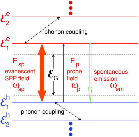
Figure 2: (Color online) Schematic illustration for a system incorporating the generation of quantum-dot excitons by a SPP field with frequency $\omega_{\rm sp}$ and probed by a plane-wave field $E_{p}$ with frequency $\omega_{p}$. Here, ${\cal E}_{\rm G}$ is the energy bandgap of the host semiconductor, $\varepsilon^{\rm e}_{\ell}$ and $\varepsilon^{\rm h}_{j}$ stand for the energy levels of electrons and holes, respectively, with $\ell,\,j=1,\,2,\,\cdots$. In addition, $\omega_{em}$ represents the frequency of spontaneous emission from photo-excited excitons, and the ground states of electrons and holes are coupled to their first excited states by lattice phonons at finite temperatures.

The physical system considered in this paper is illustrated in Fig. 2, where we assume two levels for electrons and holes, respectively, in a quantum dot. These two energy levels of both electrons and holes are efficiently coupled by phonon scattering at high temperatures. Additionally, the lowest electron and hole energy levels are optically coupled to each other by an incident SPP field to form the dressed states of excitons. The SPP-controlled optical properties of quantum-dot excitons can either probed by a plane-wave field or seen from the spontaneous emission of excitons.

For photo-excited spin-degenerated electrons in the conduction band, the semiconductor Bloch equations with $\ell=1,\,2,\,\cdots$ are given by

$$\frac{dn^{\rm e}_{\ell}}{dt}=\frac{2}{\hbar}\,\sum\limits_{j}\,{\rm Im}\left[\left(Y_{\ell}^{j}\right)^{\ast}\left({\cal M}^{\rm eh}_{\ell,j}-Y_{\ell}^{j}\,V^{\rm eh}_{\ell,j;j,\ell}\right)\right]+\left.\frac{\partial n^{\rm e}_{\ell}}{\partial t}\right|_{\rm rel}-\delta_{\ell,1}\,{\cal R}_{\rm sp}\,n_{1}^{\rm e}\,n_{1}^{\rm h}\ ,$$ (54)

where ${\cal R}_{\rm sp}$ is the spontaneous emission rate and $n^{\rm e}_{\ell}$ represents the electron level population. In Eq. (54), the term marked ‘rel’ is the non-radiative energy relaxation for $n^{\rm e}_{\ell}$, and the $Y_{\ell}^{j}$, ${\cal M}^{\rm eh}_{\ell,j}$, and $V^{\rm eh}_{\ell,j;j,\ell}$ terms are given later in the text.

Similarly, for spin-degenerate holes in the valence band, the semiconductor Bloch equations with $j=1,\,2,\,\cdots$ are found to be

$$\frac{dn^{\rm h}_{j}}{dt}=\frac{2}{\hbar}\,\sum\limits_{\ell}\,{\rm Im}\left[\left(Y_{\ell}^{j}\right)^{\ast}\left({\cal M}^{\rm eh}_{\ell,j}-Y_{\ell}^{j}\,V^{\rm eh}_{\ell,j;j,\ell}\right)\right]+\left.\frac{\partial n^{\rm h}_{j}}{\partial t}\right|_{\rm rel}-\delta_{j,1}\,{\cal R}_{\rm sp}\,n_{1}^{\rm e}\,n_{1}^{\rm h}\ ,$$ (55)

where $n^{\rm h}_{j}$ stands for the hole energy level population. Again, the non-radiative energy relaxation for $n^{\rm h}_{j}$ is incorporated in Eq. (55). Moreover, we know from Eqs. (54) and (55) that

$$N_{\rm e}(t)=2\,\sum\limits_{\ell}\,n^{\rm e}_{\ell}(t)=2\,\sum\limits_{j}\,n^{\rm h}_{j}(t)=N_{\rm h}(t)\ ,$$ (56)

where $N_{\rm e}(t)$ and $N_{\rm h}(t)$ are the total number of photo-excited electrons and holes, respectively, in the quantum dot at time $t$.

Finally, for spin-averaged e-h plasmas, the induced interband optical coherence, which is introduced in Eqs. (54) and (55), with $j=1,\,2,\,\cdots$ and $\ell=1,\,2,\,\cdots$ satisfies the following equations,

$$i\hbar\,\frac{d}{dt}Y_{\ell}^{j}=\left[\overline{\varepsilon}^{\rm e}_{\ell}(\omega)+\overline{\varepsilon}^{\rm h}_{j}(\omega)-\hbar(\omega+i\gamma_{0})\right]Y_{\ell}^{j}+\left(1-n^{\rm e}_{\ell}-n^{\rm h}_{j}\right)\left({\cal M}^{\rm eh}_{\ell,j}-Y_{\ell}^{j}\,V^{\rm eh}_{\ell,j;j,\ell}\right)$$

$$+Y_{\ell}^{j}\left[\sum\limits_{j_{1}}\,n^{\rm h}_{j_{1}}\left(V^{\rm hh}_{j,j_{1};j_{1},j}-V^{\rm hh}_{j,j_{1};j,j_{1}}\right)-\sum\limits_{\ell_{1}}\,n^{\rm e}_{\ell_{1}}\,V^{\rm eh}_{\ell_{1},j;j,\ell_{1}}\right]$$

$$+Y_{\ell}^{j}\left[\sum\limits_{\ell_{1}}\,n^{\rm e}_{\ell_{1}}\left(V^{\rm ee}_{\ell,\ell_{1};\ell_{1},\ell}-V^{\rm ee}_{\ell,\ell_{1};\ell,\ell_{1}}\right)-\sum\limits_{j_{1}}\,n^{\rm h}_{j_{1}}\,V^{\rm eh}_{\ell,j_{1};j_{1},\ell}\right]\ ,$$ (57)

where $\hbar\gamma_{0}=\hbar\gamma_{\rm eh}+\hbar\gamma_{ext}$ is the total energy-level broadening due to both the finite carrier lifetime and the loss of an external evanescent field, $\omega$ is the frequency of the external field, and $\overline{\varepsilon}^{\rm e}_{\ell}(\omega)$ and $\overline{\varepsilon}^{\rm h}_{j}(\omega)$ are the kinetic energies of dressed single electrons and holes, respectively (see Appendix A with $\alpha=1$). In Eq. (57), the diagonal dephasing ($\gamma_{0}$) of $Y^{j}_{\ell}$, the renormalization of interband Rabi coupling ($Y_{\ell}^{j}\,V^{\rm eh}_{\ell,j;j,\ell}$), the renormalization of electron and hole energies (third and fourth terms on the right-hand side), as well as the exciton binding energy, are all taken into consideration. Since the e-h plasmas are independent of spin index in this case, they can be excited by both left-circularly and right-circularly polarized light. The off-diagonal dephasing of $Y^{j}_{\ell}$ has been neglected due to low carrier density.

The steady-state solution to Eq. (57), i.e. under the condition of $dY^{j}_{\ell}/dt=0$, is found to be

$$Y^{j}_{\ell}(t|\omega)=\left[\frac{1-n^{\rm e}_{\ell}(t)-n_{j}^{\rm h}(t)}{\hbar(\omega+i\gamma_{0})-\hbar\overline{\Omega}^{\rm eh}_{\ell,j}(\omega|t)}\right]{\cal M}^{\rm eh}_{\ell,j}(t)\ ,$$ (58)

where the photon and Coulomb renormalized interband energy-level separation $\hbar\overline{\Omega}^{\rm eh}_{\ell,j}(\omega|t)$ is given by

$$\hbar\overline{\Omega}^{\rm eh}_{\ell,j}(\omega|t)=\overline{\varepsilon}^{\rm e}_{\ell}(\omega|t)+\overline{\varepsilon}^{\rm h}_{j}(\omega|t)-V^{eh}_{\ell,j;j,\ell}+\sum\limits_{\ell_{1}}\,n^{\rm e}_{\ell_{1}}(t)\left(V^{\rm ee}_{\ell,\ell_{1};\ell_{1},\ell}-V^{\rm ee}_{\ell,\ell_{1};\ell,\ell_{1}}\right)$$

$$+\sum\limits_{j_{1}}\,n^{\rm h}_{j_{1}}(t)\left(V^{\rm hh}_{j,j_{1};j_{1},j}-V^{\rm hh}_{j,j_{1};j,j_{1}}\right)-\sum\limits_{\ell_{1}\neq\ell}\,n^{\rm e}_{\ell_{1}}(t)\,V^{\rm eh}_{\ell_{1},j;j,\ell_{1}}-\sum\limits_{j_{1}\neq j}\,n^{\rm h}_{j_{1}}(t)\,V^{\rm eh}_{\ell,j_{1};j_{1},\ell}\ .$$ (59)

The steady-state solution in Eq. (58) can be substituted into Eqs. (54) and (55) above.

The Coulomb interaction matrix elements introduced in Eqs.(54), (55) and (57) are defined as

$$V^{\rm ee}_{\ell_{1},\ell_{2};\ell_{3},\ell_{4}}=\int d^{3}{\bf r}\int d^{3}{\bf r}^{\prime}\,\left[\psi^{\rm e}_{\ell_{1}}({\bf r})\right]^{\ast}\left[\psi^{\rm e}_{\ell_{2}}({\bf r}^{\prime})\right]^{\ast}\frac{e^{2}}{4\pi\epsilon_{0}\epsilon_{b}|{\bf r}-{\bf r}^{\prime}|}\,\psi^{\rm e}_{\ell_{3}}({\bf r}^{\prime})\,\psi^{\rm e}_{\ell_{4}}({\bf r})$$

$$=\frac{e^{2}}{8\pi^{2}\epsilon_{0}\epsilon_{b}}\int d^{2}{\bf q}_{\|}\,{\cal F}^{\rm e}_{\ell_{1},\ell_{4}}({\bf q}_{\|})\,{\cal F}^{\rm e}_{\ell_{2},\ell_{3}}(-{\bf q}_{\|})\left(\frac{1}{q_{\|}+q_{s}}\right)=\left(V^{\rm ee}_{\ell_{1},\ell_{2};\ell_{3},\ell_{4}}\right)^{\ast}\ ,$$ (60)

$$V^{\rm hh}_{j_{1},j_{2};j_{3},j_{4}}=\int d^{3}{\bf r}\int d^{3}{\bf r}^{\prime}\,\left[\psi^{\rm h}_{j_{1}}({\bf r})\right]^{\ast}\left[\psi^{\rm h}_{j_{2}}({\bf r}^{\prime})\right]^{\ast}\frac{e^{2}}{4\pi\epsilon_{0}\epsilon_{b}|{\bf r}-{\bf r}^{\prime}|}\,\psi^{\rm h}_{j_{3}}({\bf r}^{\prime})\,\psi^{\rm h}_{j_{4}}({\bf r})$$

$$=\frac{e^{2}}{8\pi^{2}\epsilon_{0}\epsilon_{b}}\int d^{2}{\bf q}_{\|}\,{\cal F}^{\rm h}_{j_{1},j_{4}}({\bf q}_{\|})\,{\cal F}^{\rm h}_{j_{2},j_{3}}(-{\bf q}_{\|})\left(\frac{1}{q+q_{s}}\right)=\left(V^{\rm hh}_{j_{1},j_{2};j_{3},j_{4}}\right)^{\ast}\ ,$$ (61)

$$V^{\rm eh}_{\ell,j;j^{\prime},\ell^{\prime}}=\int d^{3}{\bf r}\int d^{3}{\bf r}^{\prime}\,\left[\psi^{\rm e}_{\ell}({\bf r})\right]^{\ast}\left[\psi^{\rm h}_{j}({\bf r}^{\prime})\right]^{\ast}\frac{e^{2}}{4\pi\epsilon_{0}\epsilon_{b}|{\bf r}-{\bf r}^{\prime}|}\,\psi^{\rm h}_{j^{\prime}}({\bf r}^{\prime})\,\psi^{\rm e}_{\ell^{\prime}}({\bf r})$$

$$=\frac{e^{2}}{8\pi^{2}\epsilon_{0}\epsilon_{b}}\int d^{2}{\bf q}_{\|}\,{\cal F}^{\rm e}_{\ell,\ell^{\prime}}({\bf q}_{\|})\,{\cal F}^{\rm h}_{j,j^{\prime}}(-{\bf q}_{\|})\left(\frac{1}{q+q_{s}}\right)=\left(V^{\rm eh}_{\ell,j;j^{\prime},\ell^{\prime}}\right)^{\ast}\ ,$$ (62)

where the static screening length $1/q_{s}$ at temperatures ($k_{B}T\gg E_{F}$) is determined from

$$q_{s}(t)=\frac{e^{2}}{4\epsilon_{0}\epsilon_{b}{\cal S}\,k_{\rm B}T}\left[N_{\rm e}(t)+N_{\rm h}(t)\right]\ ,$$ (63)

${\cal S}$ is the cross-sectional area of a quantum dot, $T$ is the lattice temperature, $\psi^{\rm e}_{\ell}({\bf r})$ and $\psi^{\rm h}_{j}({\bf r})$ are the envelope wave-functions of electrons and holes in a quantum dot (see Appendix A), $\epsilon_{b}$ is the average dielectric constant of the host semiconductor. The two dimensionless form factors (see Appendix A) introduced in Eqs. (60)-(62) for electrons and holes due to quantum confinement by a quantum dot are defined by

$${\cal F}_{\ell,\ell^{\prime}}^{\rm e}({\bf q_{\|}})=e^{-q_{\|}{\cal L}_{0}}\int d^{2}{\bf r}_{\|}\left[\psi_{\ell}^{\rm e}({\bf r}_{\|})\right]^{\ast}{\rm e}^{i{\bf q}_{\|}\cdot{\bf r}_{\|}}\,\psi_{\ell^{\prime}}^{\rm e}({\bf r}_{\|})=\left[{\cal F}_{\ell,\ell^{\prime}}^{\rm e}(-{\bf q}_{\|})\right]^{\ast}\ ,$$ (64)

$${\cal F}_{j,j^{\prime}}^{\rm h}({\bf q}_{\|})=e^{-q_{\|}{\cal L}_{0}}\int d^{2}{\bf r}_{\|}\left[\psi_{j}^{\rm h}({\bf r}_{\|})\right]^{\ast}{\rm e}^{i{\bf q}_{\|}\cdot{\bf r}_{\|}}\,\psi_{j^{\prime}}^{\rm e}({\bf r}_{\|})=\left[{\cal F}_{j,j^{\prime}}^{\rm h}(-{\bf q}_{\|})\right]^{\ast}\ ,$$ (65)

where ${\cal L}_{0}$ is the thickness of a disk-like quantum dot. In addition, the matrix elements employed in Eqs. (54), (55) and (57) for the Rabi coupling between photo-excited carriers and an evanescent external field $\displaystyle{\mbox{\boldmath$E$}({\bf r};\,t)=\theta(t)\,\mbox{\boldmath$E$}({\bf r};\,\omega)\,e^{-i\omega t}}$ are given by

$${\cal M}^{\rm eh}_{\ell,j}(t)=-\delta_{\ell,1}\,\delta_{j,1}\,\theta(t)\,\left[\mbox{\boldmath$E$}^{\rm eh}_{\ell,j}(\omega)\cdot{\bf d}_{\rm c,v}\right]\ ,$$ (66)

where $\theta(x)$ is a unit step function, the static interband dipole moment ${\bf d}_{\rm c,v}$ (see Appendix A) is

$${\bf d}_{\rm c,v}=\int d^{3}{\bf r}\left[u_{\rm c}({\bf r})\right]^{\ast}\,{\bf r}\,u_{\rm v}({\bf r})={\bf d}_{\rm c,v}^{\ast}\ ,$$ (67)

$u_{\rm c}({\bf r})$ and $u_{\rm v}({\bf r})$ are the Bloch functions associated with conduction and valence bands at the $\Gamma$-point in the first Brillouin zone of the host semiconductor, and the effective electric field coupled to the quantum dot is

$$\mbox{\boldmath$E$}^{\rm eh}_{\ell,j}(\omega)=\int d^{3}{\bf r}\left[\psi^{\rm e}_{\ell}({\bf r})\right]^{\ast}\mbox{\boldmath$E$}({\bf r};\,\omega)\left[\psi^{\rm h}_{j}({\bf r})\right]^{\ast}\ .$$ (68)

The Boltzmann-type scattering term force for non-radiative electron energy relaxation in Eq. (54) is

$$\left.\frac{\partial n^{\rm e}_{\ell}}{\partial t}\right|_{\rm rel}={\cal W}_{\ell}^{({\rm in})}(1-n_{\ell}^{\rm e})-{\cal W}_{\ell}^{({\rm out})}\,n_{\ell}^{\rm e}\ ,$$ (69)

where the microscopic scattering-in and scattering-out rates are calculated as

$${\cal W}_{\ell}^{({\rm in})}=\frac{2\pi}{\hbar}\,\sum\limits_{\ell^{\prime}}\,^{\prime}\,\left|V^{\rm ep}_{\ell,\ell^{\prime}}\right|^{2}\,n^{\rm e}_{\ell^{\prime}}\left\{{\cal N}_{\rm ph}(\Omega_{0})\left[\frac{\hbar\Gamma_{\rm ph}/\pi}{(\overline{\varepsilon}^{\rm e}_{\ell}-\overline{\varepsilon}^{\rm e}_{\ell^{\prime}}-\hbar\Omega_{0})^{2}+\hbar^{2}\Gamma^{2}_{\rm ph}}\right]\right.$$

$$\left.+\left[{\cal N}_{\rm ph}(\Omega_{0})+1\right]\left[\frac{\hbar\Gamma_{\rm ph}/\pi}{(\overline{\varepsilon}^{\rm e}_{\ell}-\overline{\varepsilon}^{\rm e}_{\ell^{\prime}}+\hbar\Omega_{0})^{2}+\hbar^{2}\Gamma^{2}_{\rm ph}}\right]\right\}$$

$$+\frac{2\pi}{\hbar}\,\sum\limits_{\ell^{\prime}}\,^{\prime}\,\sum\limits_{j,j^{\prime}}\,^{\prime}\,\left|V^{\rm eh}_{\ell,j;j^{\prime},\ell^{\prime}}\right|^{2}\,(1-n_{j}^{\rm h})\,n^{\rm h}_{j^{\prime}}\,n^{\rm e}_{\ell^{\prime}}\left[\frac{\hbar\gamma_{\rm eh}/\pi}{(\overline{\varepsilon}^{\rm e}_{\ell}+\overline{\varepsilon}^{\rm h}_{j}-\overline{\varepsilon}^{\rm e}_{\ell^{\prime}}-\overline{\varepsilon}^{\rm h}_{j^{\prime}})^{2}+\hbar^{2}\gamma_{\rm eh}^{2}}\right]\ ,$$ (70)

$${\cal W}_{\ell}^{({\rm out})}=\frac{2\pi}{\hbar}\,\sum\limits_{\ell^{\prime}}\,^{\prime}\,\left|V^{\rm ep}_{\ell,\ell^{\prime}}\right|^{2}\,(1-n^{\rm e}_{\ell^{\prime}})\left\{{\cal N}_{\rm ph}(\Omega_{0})\left[\frac{\hbar\Gamma_{\rm ph}/\pi}{(\overline{\varepsilon}^{\rm e}_{\ell^{\prime}}-\overline{\varepsilon}^{\rm e}_{\ell}-\hbar\Omega_{0})^{2}+\hbar^{2}\Gamma^{2}_{\rm ph}}\right]\right.$$

$$\left.+\left[{\cal N}_{\rm ph}(\Omega_{0})+1\right]\left[\frac{\hbar\Gamma_{\rm ph}/\pi}{(\overline{\varepsilon}^{\rm e}_{\ell^{\prime}}-\overline{\varepsilon}^{\rm e}_{\ell}+\hbar\Omega_{0})^{2}+\hbar^{2}\Gamma^{2}_{\rm ph}}\right]\right\}$$

$$+\frac{2\pi}{\hbar}\,\sum\limits_{\ell^{\prime}}\,^{\prime}\,\sum\limits_{j,j^{\prime}}\,^{\prime}\,\left|V^{\rm eh}_{\ell^{\prime},j;j^{\prime},\ell}\right|^{2}\,(1-n^{\rm e}_{\ell^{\prime}})\,(1-n^{\rm h}_{j})\,n_{j^{\prime}}^{\rm h}\left[\frac{\hbar\gamma_{\rm eh}/\pi}{(\overline{\varepsilon}^{\rm e}_{\ell^{\prime}}+\overline{\varepsilon}^{\rm h}_{j}-\overline{\varepsilon}^{\rm e}_{\ell}-\overline{\varepsilon}^{\rm h}_{j^{\prime}})^{2}+\hbar^{2}\gamma_{\rm eh}^{2}}\right]\ .$$ (71)

Here,the primed summations in Eqs. (70) and (71) exclude the terms satisfying either $j=j^{\prime}$ or $\ell^{\prime}=\ell$, ${\cal N}_{\rm ph}(\Omega_{0})=[\exp(\hbar\Omega_{0}/k_{\rm B}T)-1]^{-1}$ is the Bose function for the thermal-equilibrium phonons, and $\Omega_{0}$ and $\Gamma_{\rm ph}$ are the frequency and lifetime of longitudinal-optical phonons in the host semiconductor. Similarly, the Boltzmann-type scattering term for hole non-radiative energy relaxation in Eq. (55) is

$$\left.\frac{\partial n^{\rm h}_{j}}{\partial t}\right|_{\rm rel}=\overline{{\cal W}}_{j}^{({\rm in})}(1-n_{j}^{\rm h})-\overline{{\cal W}}_{j}^{({\rm out})}\,n_{j}^{\rm h}\ ,$$ (72)

where the scattering-in and scattering-out rates are

$$\overline{{\cal W}}_{j}^{({\rm in})}=\frac{2\pi}{\hbar}\,\sum\limits_{j^{\prime}}\,^{\prime}\,\left|V^{\rm hp}_{j,j^{\prime}}\right|^{2}\,n^{\rm h}_{j^{\prime}}\left\{{\cal N}_{\rm ph}(\Omega_{0})\left[\frac{\hbar\Gamma_{\rm ph}/\pi}{(\overline{\varepsilon}^{\rm h}_{j}-\overline{\varepsilon}^{\rm h}_{j^{\prime}}-\hbar\Omega_{0})^{2}+\hbar^{2}\Gamma^{2}_{\rm ph}}\right]\right.$$

$$\left.+\left[{\cal N}_{\rm ph}(\Omega_{0})+1\right]\left[\frac{\hbar\Gamma_{\rm ph}/\pi}{(\overline{\varepsilon}^{\rm h}_{j}-\overline{\varepsilon}^{\rm h}_{j^{\prime}}+\hbar\Omega_{0})^{2}+\hbar^{2}\Gamma^{2}_{\rm ph}}\right]\right\}$$

$$+\frac{2\pi}{\hbar}\,\sum\limits_{\ell,\ell^{\prime}}\,^{\prime}\,\sum\limits_{j^{\prime}}\,^{\prime}\,\left|V^{\rm eh}_{\ell,j;j^{\prime},\ell^{\prime}}\right|^{2}\,(1-n_{\ell}^{\rm e})\,n^{\rm h}_{j^{\prime}}\,n^{\rm e}_{\ell^{\prime}}\left[\frac{\hbar\gamma_{\rm eh}/\pi}{(\overline{\varepsilon}^{\rm e}_{\ell}+\overline{\varepsilon}^{\rm h}_{j}-\overline{\varepsilon}^{\rm e}_{\ell^{\prime}}-\overline{\varepsilon}^{\rm h}_{j^{\prime}})^{2}+\hbar^{2}\gamma_{\rm eh}^{2}}\right]\ ,$$ (73)

$$\overline{{\cal W}}_{j}^{({\rm out})}=\frac{2\pi}{\hbar}\,\sum\limits_{j^{\prime}}\,^{\prime}\,\left|V^{\rm hp}_{j,j^{\prime}}\right|^{2}\,(1-n^{\rm h}_{j^{\prime}})\left\{{\cal N}_{\rm ph}(\Omega_{0})\left[\frac{\hbar\Gamma_{\rm ph}/\pi}{(\overline{\varepsilon}^{\rm h}_{j^{\prime}}-\overline{\varepsilon}^{\rm h}_{j}-\hbar\Omega_{0})^{2}+\hbar^{2}\Gamma^{2}_{\rm ph}}\right]\right.$$

$$\left.+\left[{\cal N}_{\rm ph}(\Omega_{0})+1\right]\left[\frac{\hbar\Gamma_{\rm ph}/\pi}{(\overline{\varepsilon}^{\rm h}_{j^{\prime}}-\overline{\varepsilon}^{\rm h}_{j}+\hbar\Omega_{0})^{2}+\hbar^{2}\Gamma^{2}_{\rm ph}}\right]\right\}$$

$$+\frac{2\pi}{\hbar}\,\sum\limits_{\ell,\ell^{\prime}}\,^{\prime}\,\sum\limits_{j^{\prime}}\,^{\prime}\,\left|V^{\rm eh}_{\ell,j^{\prime};j,\ell^{\prime}}\right|^{2}\,(1-n^{\rm e}_{\ell})\,(1-n^{\rm h}_{j^{\prime}})\,n_{\ell^{\prime}}^{\rm e}\left[\frac{\hbar\gamma_{\rm eh}/\pi}{(\overline{\varepsilon}^{\rm e}_{\ell}+\overline{\varepsilon}^{\rm h}_{j^{\prime}}-\overline{\varepsilon}^{\rm e}_{\ell^{\prime}}-\overline{\varepsilon}^{\rm h}_{j})^{2}+\hbar^{2}\gamma_{\rm eh}^{2}}\right]\ ,$$ (74)

and again the primed summations in Eqs. (73) and (74) exclude the terms satisfying either $j^{\prime}=j$ or $\ell=\ell^{\prime}$. The coupling between the longitudinal-optical phonons and electrons or holes in Eqs. (70), (71), (73) and (74) are calculated as

$$\left|V^{\rm ep}_{\ell,\ell^{\prime}}\right|^{2}=\frac{e^{2}\hbar\Omega_{0}}{8\pi^{2}\epsilon_{0}}\left(\frac{1}{\epsilon_{\infty}}-\frac{1}{\epsilon_{s}}\right)\int d^{2}{\bf q}_{\|}\,\left|{\cal F}^{\rm e}_{\ell,\ell^{\prime}}({\bf q}_{\|})\right|^{2}\left(\frac{1}{q_{\|}+q_{s}}\right)\ ,$$ (75)

$$\left|V^{\rm hp}_{\ell,\ell^{\prime}}\right|^{2}=\frac{e^{2}\hbar\Omega_{0}}{8\pi^{2}\epsilon_{0}}\left(\frac{1}{\epsilon_{\infty}}-\frac{1}{\epsilon_{s}}\right)\int d^{2}{\bf q}_{\|}\,\left|{\cal F}^{\rm h}_{j,j^{\prime}}({\bf q}_{\|})\right|^{2}\left(\frac{1}{q_{\|}+q_{s}}\right)\ ,$$ (76)

where $\epsilon_{\infty}$ and $\epsilon_{s}$ are the high-frequency and static dielectric constants of the host polar semiconductor.

By generalizing the Kubo-Martin-Schwinger relation, r9 the time-dependent spontaneous emission rate, ${\cal R}_{\rm sp}(t)$, introduced in Eqs. (54) and (55), can be expressed as

$${\cal R}_{\rm sp}(t)=\frac{\left|{\bf d}^{\prime}_{\rm c,v}(t)\right|^{2}}{\epsilon_{0}\sqrt{\epsilon_{b}}}\left|\int d^{3}{\bf r}\,\psi^{\rm e}_{1}({\bf r})\,\psi^{\rm h}_{1}({\bf r})\right|^{2}\int\limits_{0}^{\infty}d\omega^{\prime}\,\theta\left[\hbar\omega^{\prime}-{\cal E}_{\rm c}(t)-\overline{\varepsilon}^{\rm e}_{1}(\omega|t)-\overline{\varepsilon}^{\rm h}_{1}(\omega|t)\right]$$

$$\times\hbar\omega^{\prime}\,\rho_{0}(\omega^{\prime})\left\{\frac{\hbar\gamma_{\rm eh}}{[\hbar\omega^{\prime}-{\cal E}_{\rm c}(t)-\overline{\varepsilon}^{\rm e}_{1}(\omega|t)-\overline{\varepsilon}^{\rm h}_{1}(\omega|t)]^{2}+\hbar^{2}\gamma^{2}_{\rm eh}}\right\}\ ,$$ (77)

where

$$\left|{\bf d}^{\prime}_{\rm c,v}(t)\right|^{2}=\frac{e^{2}\hbar^{2}}{2m_{0}\,{\cal E}_{\rm G}(T)}\left[1+\frac{{\cal E}_{\rm c}(t)}{{\cal E}_{\rm G}(T)}\right]\left(\frac{m_{0}}{m_{\rm e}^{\ast}}-1\right)\ ,$$ (78)

${\cal E}_{\rm G}(T)={\cal E}_{\rm G}(0)-5.41\times 10^{-4}\,T^{2}/(T+204)$ (in units of eV) is the energy bandgap of the host semiconductor, $\rho_{0}(\omega)=\omega^{2}/c^{3}\pi^{2}\hbar$ is the density-of-states of spontaneously-emitted photons in vacuum, $m_{0}$ is the free electron mass, $m_{\rm e}^{\ast}$ is the effective mass of electrons, and the Coulomb renormalization of the energy bandgap ${\cal E}_{\rm c}(t)$ is calculated as

$${\cal E}_{\rm c}(t)=\sum\limits_{\ell_{1}}\,n^{\rm e}_{\ell_{1}}(t)\left(V^{\rm ee}_{1,\ell_{1};\ell_{1},1}-V^{\rm ee}_{1,\ell_{1};1,\ell_{1}}\right)+\sum\limits_{j_{1}}\,n^{\rm h}_{j_{1}}(t)\left(V^{\rm hh}_{1,j_{1};j_{1},1}-V^{\rm hh}_{1,j_{1};1,j_{1}}\right)$$

$$-\sum\limits_{\ell_{1}}\,n^{\rm e}_{\ell_{1}}(t)\,V^{\rm eh}_{\ell_{1},1;1,\ell_{1}}-\sum\limits_{j_{1}}\,n^{\rm h}_{j_{1}}(t)\,V^{\rm eh}_{1,j_{1};j_{1},1}-\left[1-n^{\rm e}_{1}(t)-n^{\rm h}_{1}(t)\right]\,V^{\rm eh}_{1,1;1,1}\ .$$ (79)

In Eq. (79), the first two terms are associated with the Hartree-Fock energies of electrons and holes, while the rest of the terms are related to the exciton binding energy.

Finally, the photo-induced interband optical polarization $\mbox{\boldmath${\cal P}$}^{\rm loc}({\bf r};\,\omega)$, which is related to the induced interband optical coherence, by dressed electrons in the quantum dot is given by r7

$$\mbox{\boldmath${\cal P}$}^{\rm loc}({\bf r};\,\omega)=2\left|\xi({\bf r})\right|^{2}\,{\bf d}_{\rm c,v}\left\{\int d^{3}{\bf r}^{\prime}\,\psi^{\rm e}_{1}({\bf r}^{\prime})\,\psi^{\rm h}_{1}({\bf r}^{\prime})\right\}$$

$$\times\,\frac{1}{\hbar}\,\lim\limits_{t\to\infty}\left[\frac{1-n^{\rm e}_{1}(t)-n_{1}^{\rm h}(t)}{\omega+i\gamma_{0}-\overline{\Omega}^{\rm eh}_{1,1}(\omega|t)}\right]{\cal M}^{\rm eh}_{1,1}(t)\ ,$$ (80)

where ${\bf d}_{\rm c,v}=d_{\rm c,v}\,\hat{\bf e}_{\rm d}$ represents the interband dipole moment [see Eq. (67)], $\hat{\bf e}_{\rm d}$ is the unit vector of the dipole moment, and $|\xi({\bf r})|^{2}$ comes from the confinement of a quantum dot.

II.4 Self-Consistent Field Equation

Since the wavelength of the incident light is much larger than the size of a quantum dot, we can treat the quantum dot, which is excited resonantly by the incident light, as a point dipole at ${\bf r}={\bf r}_{0}=(0,0,z_{0})$, i.e. we can assume $\mbox{\boldmath${\cal P}$}^{\rm loc}({\bf r}^{\prime};\,\omega)=\mbox{\boldmath${\cal P}$}^{\rm loc}(\omega)\,\delta({\bf r}^{\prime}-{\bf r}_{0})$ in Eq. (4) to neglect its geometry effect. This greatly simplifies the calculation and gives rise to

$$E_{\mu}({\bf r};\,\omega)=E^{(0)}_{\mu}({\bf r};\,\omega)-\frac{\omega^{2}}{\epsilon_{0}c^{2}}\sum\limits_{\nu}\,{\cal G}_{\mu\nu}({\bf r},{\bf r}_{0};\,\omega)\,{\cal P}_{\nu}^{\rm loc}(\omega)\ ,$$ (81)

where

$$\mbox{\boldmath${\cal P}$}^{\rm loc}(\omega)=2{\bf d}_{\rm c,v}\left\{\int d^{3}{\bf r}^{\prime}\,\psi^{\rm e}_{1}({\bf r}^{\prime})\,\psi^{\rm h}_{1}({\bf r}^{\prime})\right\}$$

$$\times\frac{1}{\hbar}\,\lim\limits_{t\to\infty}\left\{\frac{1-n^{\rm e}_{1}(t)-n_{1}^{\rm h}(t)}{\omega+i\gamma_{0}-\overline{\Omega}^{\rm eh}_{1,1}(\omega|t)}\right\}{\cal M}^{\rm eh}_{1,1}(t)\ ,$$ (82)

$${\cal M}^{\rm eh}_{1,1}(t)=-\theta(t)\left[\mbox{\boldmath$E$}({\bf r}_{0};\,\omega)\cdot{\bf d}_{\rm c,v}\right]\left\{\int d^{3}{\bf r}\,\psi^{\rm e}_{1}({\bf r})\,\psi^{\rm h}_{1}({\bf r})\right\}^{\ast}\ .$$ (83)

Substituting Eqs. (82) and (83) into Eq. (81), we get the following nonlinear equations for the electromagnetic field

$$E_{\mu}({\bf r};\,\omega)=E^{(0)}_{\mu}({\bf r};\,\omega)+\frac{2\omega^{2}}{\epsilon_{0}c^{2}}\left[\mbox{\boldmath$E$}({\bf r}_{0};\,\omega)\cdot{\bf d}_{\rm c,v}\right]\,d_{\rm c,v}\,\left|\int d^{3}{\bf r}^{\prime}\,\psi^{\rm e}_{1}({\bf r}^{\prime})\,\psi^{\rm h}_{1}({\bf r}^{\prime})\right|^{2}$$

$$\times\frac{1}{\hbar}\,\lim\limits_{t\to\infty}\left\{\frac{1-n^{\rm e}_{1}(t)-n_{1}^{\rm h}(t)}{\omega+i\gamma_{0}-\overline{\Omega}^{\rm eh}_{1,1}(\omega|t)}\right\}\sum\limits_{\nu}\,{\cal G}_{\mu\nu}({\bf r},{\bf r}_{0};\,\omega)\,\hat{e}_{\rm d}^{\nu}\ ,$$ (84)

where the quantum-dot level populations $n^{\rm e}_{\ell}(t)$ and $n_{j}^{\rm h}(t)$ depend nonlinearly on $\mbox{\boldmath$E$}({\bf r}_{0};\,\omega)$ in the strong-coupling regime.

If the electromagnetic field is not very strong, we can neglect the pumping effect. In this linear-response regime, we can write down the electron and hole populations in a thermal-equilibrium state [without solving Eqs. (54) and (55)]

$$n^{\rm e}_{\ell}(t)\approx f_{0}(\overline{\varepsilon}^{\rm e}_{\ell})\equiv\frac{1}{\exp[(\overline{\varepsilon}^{\rm e}_{\ell}-\mu_{\rm e})/k_{B}T]+1}\ ,$$ (85)

$$n^{\rm h}_{j}(t)\approx f_{0}(\overline{\varepsilon}^{\rm h}_{j})\equiv\frac{1}{\exp[(\overline{\varepsilon}^{\rm h}_{j}-\mu_{\rm h})/k_{B}T]+1}\ ,$$ (86)

where $f_{0}(x)$ is the Fermi function, $\mu_{\rm e}$ and $\mu_{\rm h}$ are the chemical potentials of electrons and holes, respectively, determined by Eq. (56). As a result of Eqs. (85) and (86), we get from Eq. (84) the linearized self-consistent field equation at ${\bf r}={\bf r}_{0}$

$$\sum\limits_{\nu}\,{\cal A}_{\mu\nu}({\bf r}_{0};\,\omega)\,E_{\nu}({\bf r}_{0};\,\omega)=E^{(0)}_{\mu}({\bf r}_{0};\,\omega)$$ (87)

with

$${\cal A}_{\mu\nu}({\bf r}_{0};\,\omega)=\delta_{\mu\nu}-\frac{2\omega^{2}}{\epsilon_{0}c^{2}\hbar}\left[\frac{1-f_{0}(\overline{\varepsilon}^{\rm e}_{1})-f_{0}(\overline{\varepsilon}^{\rm h}_{1})}{\omega+i\gamma_{0}-\overline{\Omega}^{\rm eh}_{1,1}(\omega)}\right]\,\left|\int d^{3}{\bf r}^{\prime}\,\psi^{\rm e}_{1}({\bf r}^{\prime})\,\psi^{\rm h}_{1}({\bf r}^{\prime})\right|^{2}$$

$$\times d^{2}_{\rm c,v}\left[\hat{e}_{\rm d}^{\nu}\sum\limits_{\nu_{1}}\,{\cal G}_{\mu\nu_{1}}({\bf r}_{0},{\bf r}_{0};\,\omega)\,\hat{e}_{\rm d}^{\nu_{1}}\right]\ ,$$ (88)

where, according to Eq. (6), we have

$${\cal G}_{\mu\nu}({\bf r}_{0},{\bf r}_{0};\,\omega)=\int\frac{d^{2}{\bf k}_{\|}}{(2\pi)^{2}}\,g_{\mu\nu}({\bf k}_{\|},\omega|z_{0},z_{0})\ .$$ (89)

The solution $\mbox{\boldmath$E$}({\bf r}_{0};\,\omega)$ of the linear-matrix equation in Eq. (87) can be substituted into Eq. (84) to find the spatial distribution of the electromagnetic field $\mbox{\boldmath$E$}({\bf r};\,\omega)$ at all positions other than ${\bf r}={\bf r}_{0}$, i.e.,

$$E_{\mu}({\bf r};\,\omega)=E^{(0)}_{\mu}({\bf r};\,\omega)+\frac{2\omega^{2}}{\epsilon_{0}c^{2}\hbar}\left[\sum\limits_{\nu,\nu^{\prime}}\,\hat{e}_{\rm d}^{\nu}\,{\cal A}^{-1}_{\nu\nu^{\prime}}({\bf r}_{0};\,\omega)\,E^{(0)}_{\nu^{\prime}}({\bf r}_{0};\,\omega)\right]$$

$$\times\left|\int d^{3}{\bf r}^{\prime}\,\psi^{\rm e}_{1}({\bf r}^{\prime})\,\psi^{\rm h}_{1}({\bf r}^{\prime})\right|^{2}\,d^{2}_{\rm c,v}\left[\frac{1-f_{0}(\overline{\varepsilon}^{\rm e}_{1})-f_{0}(\overline{\varepsilon}^{\rm h}_{1})}{\omega+i\gamma_{0}-\overline{\Omega}^{\rm eh}_{1,1}(\omega)}\right]\,\sum\limits_{\nu_{1}}\,{\cal G}_{\mu\nu_{1}}({\bf r},{\bf r}_{0};\,\omega)\,\hat{e}_{\rm d}^{\nu_{1}}\ .$$ (90)

In order to find the coupled e-h plasma and plasmon dispersion relation $\omega=\Omega_{\rm ex-pl}({\bf k}_{\|})$, we perform Fourier transforms to both $\mbox{\boldmath$E$}({\bf r};\,\omega)$ and $\mbox{\boldmath$E$}^{(0)}({\bf r};\,\omega)$ in Eq. (81) with respect to ${\bf r}_{\|}$. This leads to

$$E_{\mu}({\bf k}_{\|},\omega|x_{3})=E^{(0)}_{\mu}({\bf k}_{\|},\omega|x_{3})-\frac{\omega^{2}}{\epsilon_{0}c^{2}}\sum\limits_{\nu}\,g_{\mu\nu}({\bf k}_{\|},\omega|x_{3},z_{0})\,{\cal P}_{\nu}^{\rm loc}(\omega)\ .$$ (91)

After setting $x_{3}=z_{0}$ in Eq. (91), we get

$$\sum\limits_{\nu}\left\{\delta_{\mu\nu}-\frac{2\omega^{2}}{\epsilon_{0}c^{2}\hbar}\,\left[\frac{1-f_{0}(\overline{\varepsilon}^{\rm e}_{1})-f_{0}(\overline{\varepsilon}^{\rm h}_{1})}{\omega+i\gamma_{0}-\overline{\Omega}^{\rm eh}_{1,1}(\omega)}\right]\,\left|\int d^{3}{\bf r}^{\prime}\,\psi^{\rm e}_{1}({\bf r}^{\prime})\,\psi^{\rm h}_{1}({\bf r}^{\prime})\right|^{2}\,d^{2}_{\rm c,v}\right.$$ (92)

$$\times \left.\left[\hat{e}_{\rm d}^{\nu}\sum\limits_{\nu_{1}}\,g_{\mu\nu_{1}}({\bf k}_{\|},\omega|z_{0},z_{0})\,\hat{e}_{\rm d}^{\nu_{1}}\right]\right\}E_{\nu}({\bf k}_{\|},\omega|z_{0})=E^{(0)}_{\mu}({\bf k}_{\|},\omega|z_{0})\ .$$

Here, the zero determinant of the coefficient matrix in Eq. (92) determines the coupled e-h plasma and plasmon dispersion relation $\omega=\Omega_{\rm ex-pl}({\bf k}_{\|})$. We emphasize that the assumption of thermal-equilibrium states for electrons and holes is just for obtaining analytical expressions. Therefore, some qualitative conclusions can be drawn for guidance from these analytical solutions. Our numerical results, however, are based on the non-thermal-equilibrium steady states calculated after solving self-consistently the coupled Maxwell-Bloch equations.

By assuming an incident SPP field within the $x_{1}x_{2}$-plane, we can write

$$\mbox{\boldmath$E$}^{(0)}({\bf r};\,\omega_{\rm sp})=E_{\rm sp}\,e^{i{\bf k}_{0}(\omega_{\rm sp})\cdot{\bf D}_{0}}\,\frac{c}{\omega_{\rm sp}}\left[i\hat{\bf k}_{0}\beta_{3}(k_{0},\omega_{\rm sp})-\hat{\bf x}_{3}k_{0}(\omega_{\rm sp})\right]\,e^{i{\bf k}_{0}(\omega_{\rm sp})\cdot{\bf x}_{\|}}\,e^{-\beta_{3}(k_{0},\,\omega_{\rm sp})x_{3}}\ ,$$ (93)

where ${\bf x}_{\|}=\{x_{1},\,x_{2}\}$, $\hat{\bf k}_{0}$ and $\hat{\bf x}_{3}$ are the unit vectors in the ${\bf k}_{0}=k_{0}(\omega_{\rm sp})\{\cos\theta_{0},\,\sin\theta_{0}\}$ and $x_{3}$ directions, $E_{\rm sp}$ is the field amplitude, $\omega_{\rm sp}$ is the field frequency, $\theta_{0}$ is the angle of the incident SPP field with respect to the $x_{1}$ direction, ${\bf D}_{0}=\{-x_{g},\,-y_{g}\}$ is the position vector of the surface grating, and the two wave numbers are

$$k_{0}(\omega_{\rm sp})=\frac{\omega_{\rm sp}}{c}\sqrt{\frac{\epsilon_{\rm d}\,\epsilon_{\rm M}(\omega_{\rm sp})}{\epsilon_{\rm d}+\epsilon_{\rm M}(\omega_{\rm sp})}}\ ,$$ (94)

$$\beta_{3}(k_{0},\omega_{\rm sp})=\sqrt{k^{2}_{0}(\omega_{\rm sp})-\frac{\omega_{\rm sp}^{2}}{c^{2}}}\ ,$$ (95)

with ${\rm Re}[k_{0}(\omega_{\rm sp})]\geq 0$ and ${\rm Re}[\beta_{3}(k_{0},\omega_{\rm sp})]\geq 0$. Here, the in-plane wave number $k_{0}$ is produced by the surface-grating diffraction of the $p$-polarized normally-incident light, which in turn determines the resonant frequency $\omega$ of the SPP mode. Equation (94) stands for the full dispersion relation of the SPP field, including both radiative and non-radiative parts. From Eq. (93), it is easy to find its Fourier transformed expression

$$\mbox{\boldmath$E$}^{(0)}({\bf k}_{\|},\omega_{\rm sp}|z_{0})=\delta({\bf k}_{\|}-{\bf k}_{0})\,E_{\rm sp}\,e^{i{\bf k}_{0}(\omega_{\rm sp})\cdot{\bf D}_{0}}\,\frac{(2\pi)^{2}c}{\omega_{\rm sp}}$$

$$\times\left[i\hat{\bf k}_{0}\beta_{3}(k_{0},\omega_{\rm sp})-\hat{\bf x}_{3}k_{0}(\omega_{\rm sp})\right]\,e^{-\beta_{3}(k_{0},\,\omega_{\rm sp})z_{0}}\ .$$ (96)

II.5 Quantum-Dot Absorption

On the basis of the above electromagnetic field $\mbox{\boldmath$E$}({\bf r}_{0};\,\omega)$ at the quantum dot, we are able to compute the time-resolved nonlinear interband absorption coefficient of dressed electrons in a quantum dot for the SPP field. r11 In this case, we find

$$\beta_{0}(\omega;\,t)=\frac{\omega\sqrt{\epsilon_{b}}}{n_{\rm spp}(\omega;\,t)\,c}\left[\frac{1}{\exp(\hbar\omega/k_{\rm B}T)-1}+1\right]\,{\rm Im}\left[\alpha_{\rm spp}(\omega;\,t)\right]\ ,$$ (97)

where $\alpha_{\rm spp}(\omega;\,t)$ is the complex Lorentz function given by

$${\rm Im}[\alpha_{\rm spp}(\omega;\,t)]=\theta(t)\left(\frac{2}{\epsilon_{0}\epsilon_{b}{\cal V}|\mbox{\boldmath$E$}^{(0)}({\bf r}_{0};\,\omega)|^{2}}\right)\left|\mbox{\boldmath$E$}({\bf r}_{0};\,\omega)\cdot{\bf d}_{\rm c,v}\right|^{2}\,\left|\int d^{3}{\bf r}\,\psi^{\rm e}_{1}({\bf r})\,\psi^{\rm h}_{1}({\bf r})\right|^{2}$$

$$\times\left[1-n^{\rm e}_{1}(t)-n_{1}^{\rm h}(t)\right]\left\{\frac{[A^{2}(\omega;\,t)-B^{2}(t)]^{2}+4\hbar^{2}\gamma_{0}^{2}A^{2}(\omega;\,t)}{[A^{2}(\omega;\,t)+B^{2}(t)]^{2}+4\hbar^{2}\gamma_{0}^{2}A^{2}(\omega;\,t)}\right\}\,\left[\frac{\hbar\gamma_{0}}{\Delta^{2}(\omega;\,t)+\hbar^{2}\gamma_{0}^{2}}\right]\ ,$$ (98)

$${\rm Re}[\alpha_{\rm spp}(\omega;\,t)]=-\theta(t)\left(\frac{2}{\epsilon_{0}\epsilon_{b}{\cal V}|\mbox{\boldmath$E$}^{(0)}({\bf r}_{0};\,\omega)|^{2}}\right)\left|\mbox{\boldmath$E$}({\bf r}_{0};\,\omega)\cdot{\bf d}_{\rm c,v}\right|^{2}\,\left|\int d^{3}{\bf r}\,\psi^{\rm e}_{1}({\bf r})\,\psi^{\rm h}_{1}({\bf r})\right|^{2}$$

$$\times\left[1-n^{\rm e}_{1}(t)-n_{1}^{\rm h}(t)\right]\left\{\frac{A^{4}(\omega;\,t)-B^{4}(t)]^{2}}{[A^{2}(\omega;\,t)+B^{2}(t)]^{2}}\right\}\,\left[\frac{\Delta(\omega;\,t)}{\Delta^{2}(\omega;\,t)+\hbar^{2}\gamma_{0}^{2}}\right]\ ,$$ (99)

and the scaled refractive index function $n_{\rm spp}(\omega;\,t)$ can be calculated by

$$n_{\rm spp}(\omega;\,t)=\frac{1}{\sqrt{2}}\left(1+{\rm Re}\left[\alpha_{\rm spp}(\omega;\,t)\right]\right.$$

$$\left.+\sqrt{\left\{1+{\rm Re}\left[\alpha_{\rm spp}(\omega;\,t)\right]\right\}^{2}+\left\{{\rm Im}\left[\alpha_{\rm spp}(\omega;\,t)\right]\right\}^{2}}\,\right)^{1/2}\ .$$ (100)

In Eqs. (98) and (99), the dressed-state effects on both the level population and dipole moment have been included. In addition, we have introduced the following notations in Eqs. (98) and (99)

$$\Delta(\omega;\,t)=\sqrt{[{\cal E}_{\rm G}(T)+\varepsilon_{1}^{\rm e}+\varepsilon_{1}^{\rm h}-\hbar\omega]^{2}+4|{\cal M}^{\rm eh}_{1,1}(t)|^{2}}\ ,$$ (101)

$$A^{2}(\omega;\,t)=\left[\hbar\omega-{\cal E}_{\rm G}(T)-\varepsilon_{1}^{\rm e}-\varepsilon_{1}^{\rm h}+\Delta(\omega;\,t)\right]^{2}\ ,\ \ \ \ B^{2}(t)=4|{\cal M}^{\rm eh}_{1,1}(t)|^{2}\ .$$ (102)

II.6 Probing Quantum-Dot Dressed States

We are also able to compute the time-resolved linear interband absorption coefficient of electrons, dressed by the SPP field, for a weak probe field (not the strong SPP field) on the basis of the above calculated electromagnetic field $\mbox{\boldmath$E$}({\bf r}_{0};\,\omega)$ at the quantum dot. r11 Assuming a spatially-uniform probe field $\displaystyle{\mbox{\boldmath$E$}_{p}(t)=\theta(t-\tau)\,\mbox{\boldmath$E$}_{p}\,e^{-i\omega_{p}t}}$ with $\tau$ being the delay time, the probe-field absorption coefficient $\beta_{\rm abs}(\omega_{p};\,t)$ of the lowest dressed state is given by Eq. (97) with the replacements of $\omega$, $n_{\rm spp}$, and $\alpha_{\rm spp}$ by $\omega_{p}$, $n_{\rm pf}$, and $\alpha_{\rm pf}$, respectively, where

$$\alpha_{\rm pf}(\omega_{p};\,t)=-\theta(t-\tau)\left(\frac{2}{\epsilon_{0}\epsilon_{b}{\cal V}|\mbox{\boldmath$E$}_{p}|^{2}\hbar}\right)\left|\mbox{\boldmath$E$}_{p}\cdot{\bf d}_{\rm c,v}\right|^{2}\,\left|\int d^{3}{\bf r}\,\psi^{\rm e}_{1}({\bf r})\,\psi^{\rm h}_{1}({\bf r})\right|^{2}\,\left[1-n_{1}^{\rm e}(t)-n_{1}^{\rm h}(t)\right]$$

$$\times\left\{\frac{A^{2}(\omega;\,t)-B^{2}(t)}{[A^{2}(\omega;\,t)+B^{2}(t)]^{2}}\right\}\left\{\frac{A^{2}(\omega;\,t)}{\omega_{p}+i\gamma_{\rm eh}-\overline{\Omega}^{\rm eh}_{1,1}(\omega_{-}|t)}-\frac{B^{2}(t)}{\omega_{p}+i\gamma_{\rm eh}-\overline{\Omega}^{\rm eh}_{1,1}(\omega_{+}|t)}\right\}\ ,$$ (103)

$$n_{\rm pf}(\omega_{p};\,t)=$$

$$\frac{1}{\sqrt{2}}\left(1+{\rm Re}\left[\alpha_{\rm pf}(\omega_{p};\,t)\right]+\sqrt{\left\{1+{\rm Re}\left[\alpha_{\rm pf}(\omega_{p};\,t)\right]\right\}^{2}+\left\{{\rm Im}\left[\alpha_{\rm pf}(\omega_{p};\,t)\right]\right\}^{2}}\,\right)^{1/2}\ .$$ (104)

Here, using Eq. (59) we have

$$\hbar\overline{\Omega}^{\rm eh}_{1,1}(\omega_{\pm}|t)=\hbar\omega_{\pm}(t)-\left[1-n^{\rm e}_{1}(t)-n^{\rm h}_{1}(t)\right]V^{\rm eh}_{1,1;1,1}+\sum\limits_{\ell_{1}}\,n^{\rm e}_{\ell_{1}}(t)\left(V^{\rm ee}_{1,\ell_{1};\ell_{1},1}-V^{\rm ee}_{1,\ell_{1};1,\ell_{1}}\right)$$

$$+\sum\limits_{j_{1}}\,n^{\rm h}_{j_{1}}(t)\left(V^{\rm hh}_{1,j_{1};j_{1},1}-V^{\rm hh}_{1,j_{1};1,j_{1}}\right)-\sum\limits_{\ell_{1}}\,n^{\rm e}_{\ell_{1}}(t)\,V^{\rm eh}_{\ell_{1},1;1,\ell_{1}}-\sum\limits_{j_{1}}\,n^{\rm h}_{j_{1}}(t)\,V^{\rm eh}_{1,j_{1};j_{1},1}\ ,$$ (105)

and

$$\hbar\omega_{\pm}(t)=\hbar\omega\pm\Delta(\omega;\,t)\ .$$ (106)

Moreover, the time-resolved photoluminescence spectrum ${\cal P}_{\rm em}(\omega^{\prime};\,t)$ of dressed electrons in the quantum dot is proportional to

$${\cal P}_{\rm em}(\omega^{\prime};\,t)\propto\frac{|{\bf d}^{\prime}_{\rm c,v}|^{2}}{\epsilon_{0}\sqrt{\epsilon_{b}}{\cal L}_{0}}\,n_{1}^{\rm e}(t)\,n_{1}^{\rm h}(t)\,\hbar\gamma_{\rm eh}\,\left\{\frac{1}{[A^{2}(\omega;\,t)+B^{2}(t)]^{2}}\right\}\,\left|\int d^{3}{\bf r}\,\psi^{\rm e}_{1}({\bf r})\,\psi^{\rm h}_{1}({\bf r})\right|^{2}\,\hbar\omega^{\prime}\,\rho_{0}(\omega^{\prime})$$

$$\times\left\{\frac{A^{2}(\omega;\,t)\,B^{2}(t)}{[\hbar\omega^{\prime}-{\cal E}_{\rm c}(t)-\hbar\omega_{-}(t)]^{2}+\hbar^{2}\gamma^{2}_{\rm eh}}+\frac{A^{2}(\omega;\,t)\,B^{2}(t)}{[\hbar\omega^{\prime}-{\cal E}_{\rm c}(t)-\hbar\omega_{+}(t)]^{2}+\hbar^{2}\gamma^{2}_{\rm eh}}\right.$$

$$+\left.\frac{A^{4}(\omega;\,t)+B^{4}(t)}{[\hbar\omega^{\prime}-{\cal E}_{\rm c}(t)-\hbar\omega]^{2}+\hbar^{2}\gamma^{2}_{\rm eh}}\right\}\ .$$ (107)

III Numerical Results and Discussions

III.1 Results for the dynamics of an SPP field

In the first part of our numerical calculations, we have taken: ${\cal L}_{0}=100$ Å, $L_{y}=100$ Å, $m^{\ast}_{\rm e}=0.067\,m_{0}$, $m^{\ast}_{\rm h}=0.62\,m_{0}$, $\theta_{0}=45^{\rm o}$, $x_{g}=y_{g}=610$ Å, $\epsilon_{b}=12$, $\epsilon_{s}=11$, $\epsilon_{\infty}=13$, $\hbar\Omega_{0}=36$ meV and $\hbar\gamma_{\rm eh}=\hbar\Gamma_{\rm ph}=\hbar\gamma_{0}$. The silver plasma frequency is $13.8\times 10^{15}$ Hz and the silver plasma dephasing is $0.1075\times 10^{15}$ Hz. The energy gap $E_{\rm G}$ of the quantum-dot host material is $1.927$ eV at $T=300$ K. Other parameters, including $T$, $E_{\rm sp}$, $L_{x}$, $\hbar\gamma_{0}$, $z_{0}$ and $\epsilon_{\rm d}$, will be directly indicated in the figures.

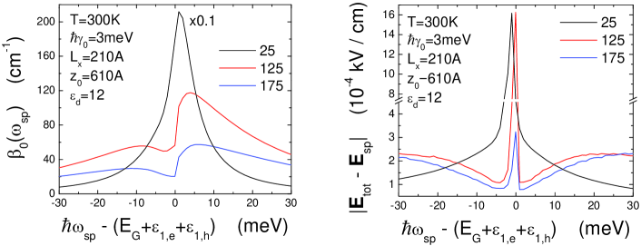
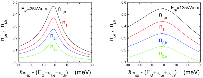
Figure 3: (Color online) Optical absorption coefficients $\beta_{0}(\omega_{\rm sp})$ (upper-left panel) and scattering field $|{\bf E}_{\rm tot}-{\bf E}_{\rm sp}|$ at the quantum dot (upper-right panel), as well as the energy-level occupations for electrons $n_{\ell,e}$ and holes $n_{j,h}$ (lower panels) with $\ell,\,j=1,\,2$, as functions of frequency detuning $\Delta\hbar\omega_{\rm sp}\equiv\hbar\omega_{\rm sp}-(E_{\rm G}+\varepsilon_{1,e}+\varepsilon_{1,h})$. Here, the results for various amplitudes $E_{\rm sp}$ of an SPP field with frequency $\omega_{\rm sp}$ are presented in the upper panels, along with a comparison of the energy-level occupations for $E_{\rm sp}=25$ and $125$ kV/cm in the lower panels. The label $\times 0.1$ in the upper-left panel indicates that the result is multiplied by a factor of $0.1$.

Figure 3 presents the quantum dot absorption coefficient $\beta_{0}(\omega_{\rm sp})$ for an SPP field, the scattering field $|{\bf E}_{\rm tot}-{\bf E}_{\rm sp}|$ of the SPP field, and the energy-level occupations for electrons $n_{\ell,e}$ and holes $n_{j,h}$ with $\ell,\,j=1,\,2$ as functions of frequency detuning $\Delta\hbar\omega_{\rm sp}\equiv\hbar\omega_{\rm sp}-(E_{\rm G}+\varepsilon_{1,e}+\varepsilon_{1,h})$. A dip is observed at resonance $\Delta\hbar\omega_{\rm sp}=0$ in the upper-left panel, which appears to become deeper with decreasing amplitude $E_{\rm sp}$ of the SPP field in the strong-coupling regime due to a decrease in the saturated absorption. However, this dip completely disappears when $E_{\rm sp}$ drops to $25$ kV/cm in the weak-coupling regime due to the suppression of the photon-dressing effect, which is accompanied by an order of magnitude increase in the absorption-peak strength. The dip in the upper-left panel corresponds to a peak in the scattering field, as can be seen from the upper-right panel of the figure. The scattering field increases with frequency detuning away from resonance, corresponding to the decreasing absorption. As a result, two minima show up on both sides of resonance for the scattering field in the strong-coupling regime. Maxwell-Bloch equations couple the field dynamics outside of a quantum dot with the electron dynamics inside the dot. At $E_{\rm sp}=125$ kV/cm in the lower-right panel, we find peaks in energy-level occupations at resonance, which are broadened by the finite carrier lifetime as well as the optical power of the SPP field. Moreover, jumps in the energy-level occupations can be seen at resonance due to Rabi splitting of the energy levels in the dressed electron states. The effect of resonant phonon absorption also plays a significant role in the finite value of $n_{2,e}$ with energy-level separations $\varepsilon_{2,e}-\varepsilon_{1,e}\approx\hbar\Omega_{0}$. However, as $E_{\rm sp}$ decreases to $25$ kV/cm in the lower-left panel, peaks in the energy-level occupations are greatly sharpened and negatively shifted due to the suppression of the broadening from the optical power and the excitonic effect, respectively. Additionally, jumps in the energy-level occupations become invisible because the Rabi-split energy gap in this case is much smaller than the energy-level broadening from the finite lifetime of electrons (i.e. severely damped Rabi oscillations between the first electron and hole levels).

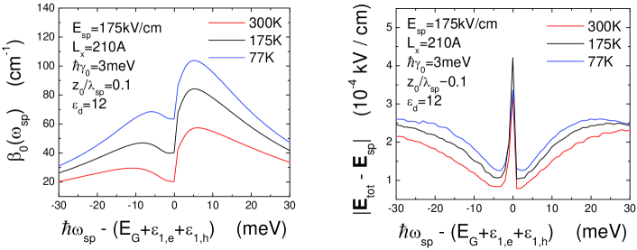
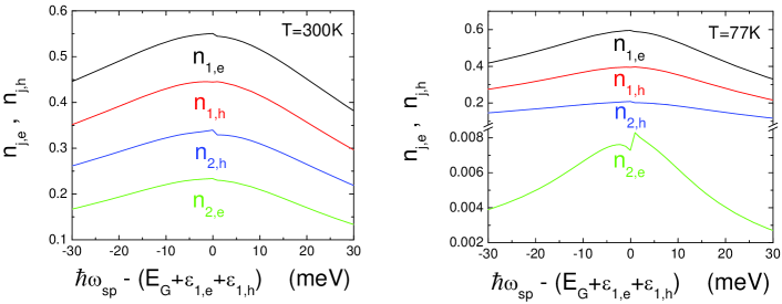
Figure 4: (Color online) $\beta_{0}(\omega_{\rm sp})$ (upper-left panel) and $|{\bf E}_{\rm tot}-{\bf E}_{\rm sp}|$ (upper-right panel), as well as $n_{\ell,e}$ and holes $n_{j,h}$ (lower panels), as functions of $\Delta\hbar\omega_{\rm sp}$. Here, the results for three different temperatures $T=300$, $175$ and $77$ K are displayed in the upper panels, along with a comparison of $n_{\ell,e}$ and holes $n_{j,h}$ for $T=300$ and $77$ K in the lower panels.

We know that a decrease in temperature $T$ gives rise to an increase in the crystal bandgap $E_{\rm G}$. On the other hand, the localization of an SPP field (i.e. an exponential decay of the field strength on either side of a metallic surface) is greatly enhanced when the SPP frequency $\omega_{\rm sp}$ approaches that of a surface plasmon. As a result, the field at the quantum dot is expected to decrease as $T$ is reduced. This gives rise to a higher absorption coefficient for a lower temperature, as shown in the upper-left panel of Fig. 4. Interestingly, although the suppressed absorption coefficient can be seen from $\beta_{0}(\omega_{\rm sp})$ for high SPP-field amplitudes, as shown by Eq. (98), from the upper-right panel of this figure we find the resonant peak at $\hbar\omega_{\rm sp}=E_{\rm G}+\varepsilon_{\rm 1,e}+\varepsilon_{\rm 1,h}$ initially increases with $T$ but then decreases with $T$ at room temperature. This subtle difference demonstrates the effect of reduced phonon absorption at $T=77$ K on the resonant scattering field by the factor $1-n_{\rm e}(t)-n_{\rm h}(t)$ in Eq. (84). Moreover, the strong effect of the suppressed optical-phonon absorption between two electron energy levels at $77$ K is clearly demonstrated in the lower panels of Fig. 4, where the level occupation $n_{\rm 2,e}$ becomes negligible at $T=77$ K in comparison with that at $T=300$ K.

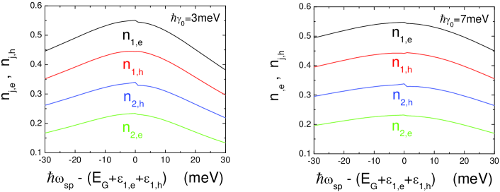
Figure 5: (Color online) $\beta_{0}(\omega_{\rm sp})$ (upper-left panel) and $|{\bf E}_{\rm tot}-{\bf E}_{\rm sp}|$ (upper-right panel), as well as $n_{\ell,e}$ and holes $n_{j,h}$ (lower panels), as functions of $\Delta\hbar\omega_{\rm sp}$. Here, the results with different energy-level broadening $\hbar\gamma_{0}=3$, $5$ and $7$ meV are shown in the upper panels, along with a comparison of $n_{\ell,e}$ and holes $n_{j,h}$ for $\hbar\gamma_{0}=3$ and $7$ meV in the lower panels.

The electron thermal dynamics due to phonon absorption has been demonstrated in Fig. 4 for various temperatures. In Fig. 5, we present the electron dynamics resulting from the optical dephasing, due to the finite lifetime of electrons, at different energy-level broadenings $\hbar\gamma_{0}$. As $\hbar\gamma_{0}$ is increased from $3$ meV to $7$ meV, the dip in $\beta_{0}(\omega_{\rm sp})$ at resonance is suppressed, leading to a single peak with a reduced strength and an increased width, as shown in the upper-left panel of the figure. This increase in the resonant absorption is further accompanied by an enhanced resonant peak for the scattering field in the upper-right panel of this figure. As expected, the energy-level occupations at $\hbar\gamma_{0}=7$ meV become much broader than those at $\hbar\gamma_{0}=3$ meV, as displayed in the lower two panels of the figure.

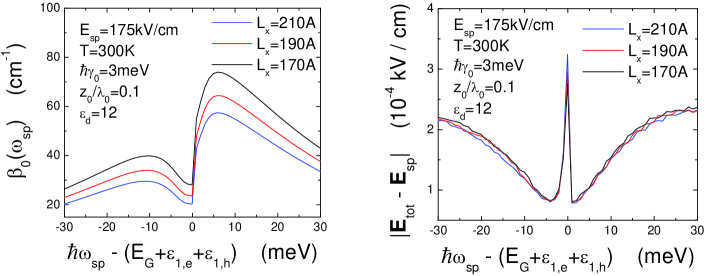
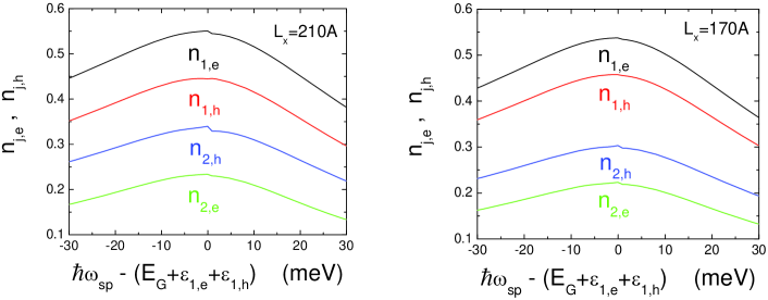
Figure 6: (Color online) $\beta_{0}(\omega_{\rm sp})$ (upper-left panel) and $|{\bf E}_{\rm tot}-{\bf E}_{\rm sp}|$ (upper-right panel), as well as $n_{\ell,e}$ and holes $n_{j,h}$ (lower panels), as functions of $\Delta\hbar\omega_{\rm sp}$. Here, the results for three different sizes $L_{x}=210$, $190$ and $170$ Å of a quantum dot are shown in the upper panels, along with a comparison of $n_{\ell,e}$ and holes $n_{j,h}$ for $L_{x}=210$ and $170$ Å in the lower panels.

We further notice that the effective bandgap $E_{\rm G}+\varepsilon_{\rm 1,e}+\varepsilon_{\rm 1,h}$ also depends on the size $L_{x}$ of a quantum dot due to the quantization effect, and the effective bandgap will increase with decreasing $L_{x}$. The size effect from such an $L_{x}$ dependence is displayed in Fig. 6. From the upper-left panel of Fig. 6, we find that the peak of $\beta_{0}(\omega_{\rm sp})$ is enhanced as $L_{x}$ is reduced. This phenomenon is connected to the increased localization of the SPP field at $L_{x}=170$ Åas the SPP frequency approaches the saturation part of its dispersion. Moreover, the dip in $\beta_{0}(\omega_{\rm sp})$ is lifted somewhat uniformly at the same time due to decreased $n_{1}^{\rm e}(t)$ from the enhanced Coulomb and phonon scattering at $L_{x}=170$ Å. Here, $\beta_{0}(\omega_{\rm sp})$ is proportional to the population factor $1-n^{\rm e}_{1}(t)-n_{1}^{\rm h}(t)$, as can be seen from Eq. (98). Besides the slightly-reduced resonant peak strength of the scattering field for $L_{x}=170$ Å (also resulting from the enhanced carrier scattering), $|{\bf E}_{\rm tot}-{\bf E}_{\rm sp}|$ keeps the same peak position, as shown in the upper-right panel of the figure. In this case, $|{\bf E}_{\rm tot}-{\bf E}_{\rm sp}|$ at the dot approaches a nonzero value at resonance, as can be seen from Eq. (90), and tends to zero rapidly away from resonance. Additionally, $n_{\rm 2,h}$ is reduced for $L_{x}=170$ Å, as can be found from a comparison between the two lower panels of the figure. This is attributed to the reduced phonon absorption between two hole energy levels.

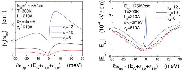
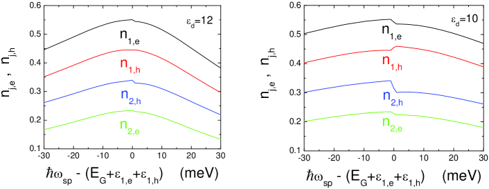
Figure 7: (Color online) $\beta_{0}(\omega_{\rm sp})$ (upper-left panel) and $|{\bf E}_{\rm tot}-{\bf E}_{\rm sp}|$ (upper-right panel), as well as $n_{\ell,e}$ and holes $n_{j,h}$ (lower panels), as functions of $\Delta\hbar\omega_{\rm sp}$. Here, the results for three dielectric constants of a cladding layer, with $\epsilon_{\rm d}=8$, $10$ and $12$, are displayed in the upper panels, along with a comparison of $n_{\ell,e}$ and holes $n_{j,h}$ for $\epsilon_{\rm d}=12$ and $10$ in the lower panels.

In Figs. 4 and 6, we vary the localization of an SPP field by changing the effective bandgap. Since the frequency of the surface plasmon (saturated dispersion part) is proportional to the factor of $1/\sqrt{1+\epsilon_{\rm d}}$, a smaller value of $\epsilon_{\rm d}$ implies a higher surface-plasmon frequency or a reduced localization of the SPP field. We verify the change in the SPP localization by observing the upper two panels of Fig. 7, where the absorption peak, as well as the resonant scattering-field peak, become much stronger as $\epsilon_{\rm d}$ is increased from $8$ to $12$ due to the reduction of saturated absorption for a lower field strength at the quantum dot. Furthermore, from the two lower panels of this figure we also observe, via the jumps in the population curves, an enhanced Rabi-split energy gap in the electron dressed states as $\epsilon_{\rm d}$ is reduced from $12$ to $10$ due to the enhanced field strength at the quantum dot.

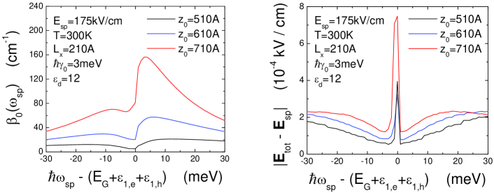
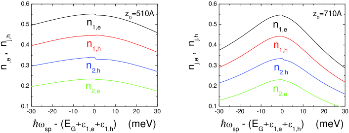
Figure 8: (Color online) $\beta_{0}(\omega_{\rm sp})$ (upper-left panel) and $|{\bf E}_{\rm tot}-{\bf E}_{\rm sp}|$ (upper-right panel), as well as $n_{\ell,e}$ and holes $n_{j,h}$ (lower panels), as functions of $\Delta\hbar\omega_{\rm sp}$. Here, the results for different vertical distances of a quantum dot from a metallic surface are displayed in the upper panels for $z_{0}=510$, $610$ and $710$ Å, along with a comparison of $n_{\ell,e}$ and holes $n_{j,h}$ for $z_{0}=510$ and $710$ Å in the lower panels.

In the presence of the localization of an SPP field, we can move a quantum dot closer to a metallic surface to gain a higher field at the quantum dot. The upper-left panel of Fig. 8 has elucidated this fact, in which a larger $z_{0}$ corresponds to a weaker field, and then, a higher absorption peak due to the reduction of saturated absorption. This fact is also reflected in the upper-right panel of the figure, where a higher resonant scattering-field peak occurs for a larger value of $z_{0}$. At $z_{0}=510$ Å, a Rabi-split energy gap at resonance is clearly visible from the lower-left-panel of the figure for electron dressed states. Additionally, at $z_{0}=710$ Å, by entering into a weak-coupling regime for a weaker field at the dot, we find sharpened resonant peaks in the energy-level occupations of electrons and holes, similar to the observation from the lower-left panel of Fig. 3.

III.2 Results for the dressed states of electrons

In the second part of the numerical calculations, besides the parameters given in the first subsection, we have fixed $L_{x}=210$ Å, $\hbar\gamma_{0}=3$ meV, $z_{0}=610$ Å and $\epsilon_{\rm d}=12$. Other parameters, including $T$, $E_{\rm sp}$ and $\Delta\hbar\omega_{\rm sp}$, will be directly indicated in the figures. Additionally, $\Delta\hbar\omega_{\rm sp}$ is given with respect to the energy gap at $T=300$ K.

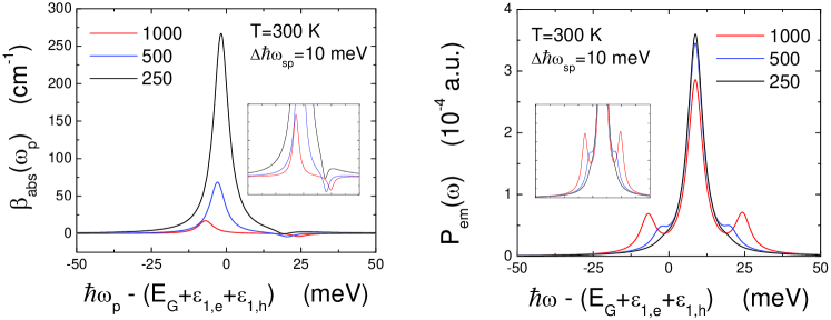
Figure 9: (Color online) Probe-field absorption coefficient $\beta_{\rm abs}(\omega_{\rm p})$ (left panel) and spontaneous emission of a quantum dot $P_{\rm em}(\omega)$ (right panel) as a function of $\hbar\omega_{\rm p}-(E_{\rm G}+\varepsilon_{\rm 1,e}+\varepsilon_{\rm 1,h})$ and $\hbar\omega-(E_{\rm G}+\varepsilon_{\rm 1,e}+\varepsilon_{\rm 1,h})$, respectively, are presented. Here, comparisons of the results with three values of SPP-field amplitudes $E_{\rm sp}=250$, $500$ and $1000$ kV/cm are given. The insets of both panels are enlarged views of the peaks.

From the left panel of Fig. 9 we find a strong absorption (positive) peak and a weak gain (negative) peak for the probe-field absorption coefficient $\beta_{\rm abs}(\omega_{\rm p})$ due to a quantum coherence effect from the electron states being dressed by an SPP field. In the strong-coupling regime, the dispersion of the quantum-dot e-h plasmas (dot-like branch) and SPPs (photon-like branch) form an anticrossing gap, where a higher-energy dot-like branch at a negative frequency detuning switches to a photon-like branch for a positive detuning. The positive peak is associated with the absorption of a probe-field photon by a quantum-dot e-h plasma, while the negative peak relates to the process with absorption of two photons from an SPP field and emission of one probe-field photon. The absorption peak is significantly reduced by saturation at $E_{\rm sp}=1000$ kV/cm, and the gain peak is suppressed by a smaller Rabi-coupling frequency at $E_{\rm sp}=250$ kV/cm (see the inset of the left panel). In addition, we observe from the right panel of Fig. 9 that two Rabi-splitting-induced side emission peaks for the spontaneous emission $P_{\rm em}(\omega)$ become weaker and closer to the strong central peak as $E_{\rm sp}$ is reduced (see the inset of the right panel). Moreover, the strength of the central peak due to the coherent conversion of an absorbed SPP-field photon to a spontaneously-emitted photon (non-linear optical behavior) is slightly reduced at $E_{\rm sp}=1000$ kV/cm as a result of saturated absorption of the SPP field.

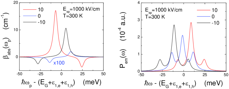
Figure 10: (Color online) $\beta_{\rm abs}(\omega_{\rm p})$ (left panel) and $P_{\rm em}(\omega)$ (right panel) as a function of $\hbar\omega_{\rm p}-(E_{\rm G}+\varepsilon_{\rm 1,e}+\varepsilon_{\rm 1,h})$ and $\hbar\omega-(E_{\rm G}+\varepsilon_{\rm 1,e}+\varepsilon_{\rm 1,h})$, respectively, are displayed. Here, we show the comparisons with three values of SPP-field detunings $\Delta\hbar\omega_{\rm sp}=0$ and $\pm 10$ meV. The label $\times 100$ for zero SPP-field detuning indicates the result is multiplied by a factor of $100$.

Figure 10 demonstrates the effect of frequency detuning $\Delta\hbar\omega_{\rm sp}$ of an SPP field with respect to the bandgap of a quantum dot. The switching of the detuning from $10$ meV to $-10$ meV reveals the corresponding spectral-position interchange between the absorption (dot-like branch) and the gain (photon-like branch) peaks for $\beta_{\rm abs}(\omega_{\rm p})$ in the left panel of the figure. The Rabi oscillations between the first electron and hole energy levels are weakened with increasing $|\Delta\hbar\omega_{\rm sp}|$. At resonance with a zero detuning, both the absorption and gain peaks are suppressed by very strong Rabi oscillations. This detuning also shifts the emission peaks correspondingly because of the coherent conversion of an SPP-field photon to a spontaneously-emitted one, as can been seen from the right panel of this figure. Moreover, the central peak is weakened and the two side peaks are enlarged at resonance as a result of energy transfer to the side peaks by strong coupling and enhanced Rabi oscillations, respectively.

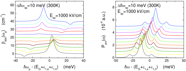
Figure 11: (Color online) $\beta_{\rm abs}(\omega_{\rm p})$ (left panel) and $P_{\rm em}(\omega)$ (right panel) as a function of $\hbar\omega_{\rm p}-(E_{\rm G}+\varepsilon_{\rm 1,e}+\varepsilon_{\rm 1,h})$ and $\hbar\omega-(E_{\rm G}+\varepsilon_{\rm 1,e}+\varepsilon_{\rm 1,h})$, respectively, are shown. Here, a series of offset curves are displayed for various temperatures from $T=250$ K (bottom black curves) to $T=300$ K (top blue curves) in steps of $5$ K.

Since the temperature affects the crystal bandgap energy $E_{\rm G}$, by changing the temperature we are able to scan the detuning $\Delta\hbar\omega_{\rm sp}$ of the SPP field with a fixed SPP frequency $\hbar\omega_{\rm sp}$ from negative to positive or vice versa. This leads to a spectral-position interchange between the absorption and gain peaks, similar to Fig. 10. The results in Fig. 11 prove such an expected feature by increasing $T$ from $250$ to $300$ K in steps of $5$ K. Technically, changing the temperature in the experiment is much easier than changing the tuning of a laser frequency over a large range. Here, the shift of the central peak in the right panel of the figure directly reflects the variation of the SPP-field detuning with $T$. Furthermore, the interchange between the dot-like and photon-like modes with $T$ in the left panel can be regarded as direct evidence for the existence of an anticrossing energy gap resulting from a strongly-coupled e-h plasma and SPP field or coupled e-h plasmas and surface plasmons.

III.3 Time-resolved optical spectra

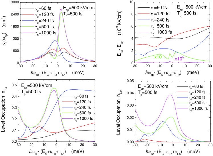
Figure 12: (Color online) $\beta_{0}(\omega_{\rm sp})$ (upper-left panel) and $|{\bf E}_{\rm tot}-{\bf E}_{\rm sp}|$ (upper-right panel), as well as $n_{1,e}$ and holes $n_{2,e}$ (lower panels), as functions of $\Delta\hbar\omega_{\rm sp}$ at different detection times $\tau_{0}$ for a Gaussian-shape laser pulse with pulse width $T_{p}=500$ fs. Here, $E_{\rm sp}=500$ kV/cm is taken, and the other parameters are the same as those in Fig. 3. The labels $\times 10$ and $\times 10^{5}$ in the upper-right panel indicate that the results are multiplied by factors of $10$ and $10^{5}$, respectively.

In our previously presented numerical results, we only showed steady-state dynamics of photo-excited e-h plasmas in a quantum dot by using a continuous SPP field, where the effects of both phonon scattering and e-h pair radiative recombination are combined with each other. Using a laser pulse to launch a pulsed SPP field, we are able to study the dynamics of phonon scattering (narrow pulse) as well as the dynamics of e-h pair radiative recombination (wide pulse), separately. Dynamically, phonon scattering becomes effective only after a characteristic time (around $1$ ps), its effect can be seen from a significant increase of $n_{\rm 2,e}$ in our system. Figure 12 displays the results for $\beta_{0}(\omega_{\rm sp})$ (upper-left), $|{\bf E}_{\rm tot}-{\bf E}_{\rm sp}|$ (upper-right), $n_{\rm 1,e}$ (lower-left) and $n_{\rm 2,e}$ (lower-right) for various detection times $\tau_{0}$ in the presence of a narrow laser pulse (with pulse width $T_{p}=500$ fs and peak value $E_{\rm sp}=500$kV/cm) which is turned on at $t=0$. We see from Fig. 12 that $\beta_{0}(\omega_{\rm sp})$ starts with a dip for the dressed state at resonance, then shifts to a single peak (at half-pulse width) due to a suppression of the photon-dressing effect. It eventually becomes a single peak plus a shifted dip after the pulse has passed due to formation of resonant peaks in $n_{\rm 1,e}$ and $n_{\rm 1,h}$. Correspondingly, $|{\bf E}_{\rm tot}-{\bf E}_{\rm sp}|$ starts by showing a non-resonant behavior with a relatively large magnitude, then shifts to a quasi-resonant behavior, and finally looks like suppressed resonant behavior with a peak at and dips on both sides of $\Delta\hbar\omega_{\rm sp}=0$. The resonant build up of $n_{\rm 1,e}$ after $\tau_{0}\geq 500$ fs can also be verified from this figure, which is accompanied by the start of significant phonon absorption after $\tau_{0}\geq 1$ ps.

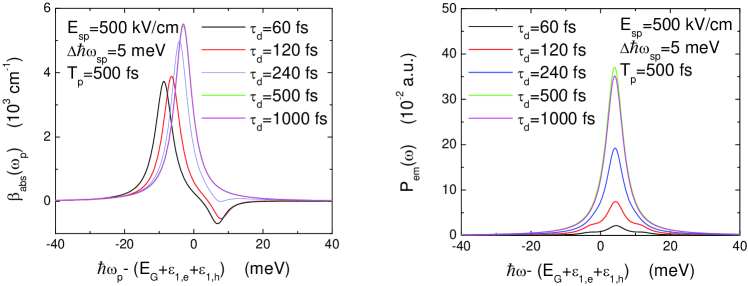
Figure 13: (Color online) $\beta_{\rm abs}(\omega_{\rm p})$ (left panel) and $P_{\rm em}(\omega)$ (right panel) as a function of $\hbar\omega_{\rm p}-(E_{\rm G}+\varepsilon_{\rm 1,e}+\varepsilon_{\rm 1,h})$ and $\hbar\omega-(E_{\rm G}+\varepsilon_{\rm 1,e}+\varepsilon_{\rm 1,h})$, respectively, at different delayed times $\tau_{d}$ for a Gaussian-shape laser pulse with pulse width $T_{p}=500$ fs. Here, $E_{\rm sp}=500$ kV/cm and $\Delta\hbar\omega_{\rm sp}=5$ meV are chosen, and the other parameters are the same as those in Fig. 3.

Technically, detecting dynamics of photo-excited e-h plasmas by using another time-delayed weak probe field is much more feasible, as shown in Fig. 13. From the left panel of this figure, we find that $\beta_{\rm abs}(\omega_{\rm p})$ starts with a pair of positive absorption and negative gain peaks due to a very strong photon dressing effect for the delayed times $\tau_{d}=60$ and $120$ fs. This is changed to a strong absorption peak plus a very weak gain peak at $\tau_{d}=240$ fs. At the end, $\beta_{\rm abs}(\omega_{\rm p})$ becomes independent of $\tau_{d}$, indicating that a linear optical-response regime has been reached. On the other hand, from the right panel of this figure, we see that the central peak of $P_{\rm em}(\omega)$ is gradually built up with increasing $\tau_{d}$ due to enhanced $n_{\rm 1,e}$ and $n_{\rm 1,h}$ around resonance, while two side peaks become weakened and disappear at the same time due to weakened Rabi oscillations. Interestingly, we also find that the central peak of $P_{\rm em}(\omega)$ slightly decreases at $\tau_{d}=1$ ps, which agrees with the observed start of significant phonon absorption seen in the lower-left panel of Fig. 12.

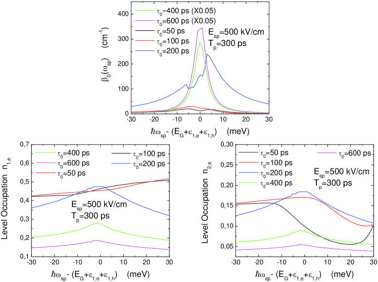
Figure 14: (Color online) $\beta_{0}(\omega_{\rm sp})$ (upper-middle panel), $n_{1,e}$ and holes $n_{2,e}$ (lower two panels), as functions of $\Delta\hbar\omega_{\rm sp}$ at different detection times $\tau_{0}$ for a wide laser pulse with pulse width $T_{p}=300$ ps. Here, $E_{\rm sp}=500$ kV/cm is taken, and the other parameters are the same as those in Fig. 3. The labels $\times 0.05$ in the upper-middle panel indicate that the results in the upper panel for $\tau_{0}=60$ and $120$ ps are multiplied by a factor of $0.05$.

In order to explore the dynamics of e-h pair radiative recombination in our system, a wide pulse with a full-pulse width around $300$ ps is required, as displayed in Fig. 14. From the upper-middle panel of this figure, we find that $\beta_{0}(\omega_{\rm sp})$ starts with a resonant dip due to a strong photon dressing effect, then shifts to a sole peak at $\Delta\hbar\omega_{\rm sp}=0$ as $\tau_{0}\geq 400$ ps where a steady state is almost reached in the linear-response regime. Accordingly, the level populations $n_{\rm 1,e}$ and $n_{\rm 2,e}$ in the lower two panels show a transition from an initial non-resonant behavior to a final resonant behavior. This is accompanied by dramatically reduced level populations due to the start of a radiative recombination process for photo-excited e-h pairs.

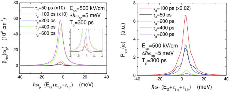
Figure 15: (Color online) $\beta_{\rm abs}(\omega_{\rm p})$ (left panel) and $P_{\rm em}(\omega)$ (right panel) as a function of $\hbar\omega_{\rm p}-(E_{\rm G}+\varepsilon_{\rm 1,e}+\varepsilon_{\rm 1,h})$ and $\hbar\omega-(E_{\rm G}+\varepsilon_{\rm 1,e}+\varepsilon_{\rm 1,h})$, respectively, at different delayed times $\tau_{d}$ for a Gaussian-shape laser pulse with pulse width $T_{p}=300$ ps. Here, $E_{\rm sp}=500$ kV/cm and $\Delta\hbar\omega_{\rm sp}=5$ meV are assumed, and the other parameters are the same as those in Fig. 3. The inset in the upper-left panel shows an enlarged view for the gain and absorption peaks for small delayed times. The labels $\times 10$ for $\tau_{d}=50$ and $100$ ps in the left panel, as well as the label $\times 0.02$ in the right panel, indicate that the results are multiplied by a factor of $10$ and a factor of $0.02$, respectively.

Recombination dynamics for e-h plasmas can also be demonstrated clearly by the time-delayed probe-field absorption as well as by the time-resolved spontaneous emission, as shown in Fig. 15. As presented in the left panel of this figure, we find that the initial weak absorption and gain peaks (see the inset) in $\beta_{\rm abs}(\omega_{\rm p})$ occur at $\tau_{d}=200$ ps and are replaced by a strong single absorption peak due to a suppressed photon dressing effect and phase-space blocking. On the other hand, from the right panel of the same figure, we see that the initial central peak in $P_{\rm em}(\omega)$ is increased very rapidly due to accumulation of photo-excited e-h pairs and accompanied by the reduction of two side peaks resulting from the weakened Rabi oscillations. Importantly, the very-strong central peak in $P_{\rm em}(\omega)$ is significantly reduced at $\tau_{d}=200$ ps, indicating the start of a radiative-recombination process for photo-excited e-h plasmas. This recombination process is continuously enhanced with the increasing delay time $\tau_{d}$ and suppresses the central peak in $P_{\rm em}(\omega)$ after $\tau_{d}\geq 400$ ps due to draining out the photo-generated electrons and holes at the same time.

IV Conclusions and Remarks

In conclusion, we have demonstrated the possibility of using a SPP field to control the optical gain and absorption of another passing light beam due to their strong nonlinear field coupling mediated by electrons in the quantum dot. We have also predicted the coherent conversion of a surface-plasmon-field photon to a spontaneously-emitted free-space photon, which is simultaneously accompanied by another pair of blue- and red-shifted photons.

Although we studied only the coupling of a SPP field to a single quantum dot in this paper for the simplest case, our formalism can be generalized easily to include many quantum dots. The numerically-demonstrated unique control of the effective photon-photon coupling by the quantum dot can be used for constructing an optical transistor, where the ‘gate’ photon controls the intensity of its ‘source’ light beam. These optical transistors are very useful for speeding up and improving the performance of fiber-optic communication networks, as well as for constructing quantum information and developing optical digital computers.

Furthermore, instead of a resonant coupling to the lowest pair of electron-hole energy levels, we may select the surface-plasmon frequency for resonant coupling to the higher pair of electron-hole levels. In such a case, the optical pumping from the intense surface-plasmon near-field could create a population inversion with respect to the ground pair of electron-hole levels by emitting thermal phonons, leading to a possible lasing action if the optical gain can overcome the metal loss for the surface plasmons. Such a surface-plasmon quantum-dot laser would have a beam size as small as a few nanometers beyond the optical diffraction limit, and it is expected to be very useful for spatially-selective illumination of individual molecules or neuron cells in low-temperature photo-excited chemical reactions or optogenetics and neuroscience.

Appendix A Electronic States of a Quantum Dot

We have employed a box-type potential with hard walls for a quantum dot, which is given by

$$V({\bf r})=\left\{\begin{array}[]{ll}0\ ,&\mbox{$0\leq x_{i}\leq L_{i}$ for $i=1,\,2,\,3$}\\ \infty\ ,&\mbox{others}\end{array}\right.\ ,$$ (108)

where the position vector ${\bf r}=(x_{1},x_{2},x_{3})$, $L_{1}$, $L_{2}$ and $L_{3}$ are the widths of the potential in the $x_{1}$, $x_{2}$ and $x_{3}$ directions, respectively. The Schrödinger equation for a single electron or hole in a quantum dot is written as

$$-\frac{\hbar^{2}}{2m^{\ast}}\left[\frac{\partial^{2}}{\partial x_{1}^{2}}+\frac{\partial^{2}}{\partial x_{2}^{2}}+\frac{\partial^{2}}{\partial x_{3}^{2}}+V({\bf r})\right]\psi({\bf r})=\varepsilon\,\psi({\bf r})\ ,$$ (109)

where the effective mass $m^{\ast}$ is $m^{\ast}_{\rm e}$ for electrons or $m^{\ast}_{\rm h}$ for holes. The eigenstate wave-function associated with Eq. (109) is found to be

$$\psi_{n_{1},n_{2},n_{3}}({\bf r})=\sqrt{\frac{2}{L_{1}}}\,\sin\left[\left(\frac{n_{1}\pi}{L_{1}}\right)x_{1}\right]\sqrt{\frac{2}{L_{2}}}\,\sin\left[\left(\frac{n_{2}\pi}{L_{2}}\right)x_{2}\right]\sqrt{\frac{2}{L_{3}}}\,\sin\left[\left(\frac{n_{3}\pi}{L_{3}}\right)x_{3}\right]\ ,$$ (110)

which is same for both electrons and holes, and the eigenstate energy associated with Eq. (109) is

$$\varepsilon_{n_{1},n_{2},n_{3}}=\frac{\hbar^{2}}{2m^{\ast}}\left[\left(\frac{n_{1}\pi}{L_{1}}\right)^{2}+\left(\frac{n_{2}\pi}{L_{2}}\right)^{2}+\left(\frac{n_{3}\pi}{L_{3}}\right)^{2}\right]\ ,$$ (111)

where the quantum numbers $n_{1},\,n_{2},\,n_{3}=1,\,2,\,\cdots$.

By using the calculated bare energy levels in Eq. (111), the dressed electron ($\lambda^{\rm e}_{\alpha}$) and hole ($\lambda^{\rm h}_{\alpha}$) energy levels under the rotating wave approximation take the form of r7

$$\lambda^{\rm e}_{\alpha}(\omega|t)=\lambda^{\rm h}_{\alpha}(\omega|t)=\left\{\begin{array}[]{cc}\frac{1}{2}\left(\hbar\omega+\sqrt{[{\cal E}_{\rm G}(T)+\varepsilon_{\alpha}^{\rm e}+\varepsilon_{\alpha}^{\rm h}-\hbar\omega]^{2}+4|{\cal M}^{\rm eh}_{\alpha,\alpha}(t)|^{2}}\,\right)&\\ \mbox{if $\hbar\omega\leq{\cal E}_{\rm G}(T)+\varepsilon_{\alpha}^{\rm e}+\varepsilon_{\alpha}^{\rm h}$}\\ \\ \frac{1}{2}\left(\hbar\omega-\sqrt{[{\cal E}_{\rm G}(T)+\varepsilon_{\alpha}^{\rm e}+\varepsilon_{\alpha}^{\rm h}-\hbar\omega]^{2}+4|{\cal M}^{\rm eh}_{\alpha,\alpha}(t)|^{2}}\,\right)&\\ \mbox{if $\hbar\omega\geq{\cal E}_{\rm G}(T)+\varepsilon_{\alpha}^{\rm e}+\varepsilon_{\alpha}^{\rm h}$}\end{array}\right.\ ,$$ (112)

where the composite index $\alpha=\{n_{1},\,n_{2},\,n_{3}\}$. Moreover, we get the energy levels of dressed electrons $\overline{\varepsilon}^{\rm e}_{\alpha}(\omega|t)=\lambda^{\rm e}_{\alpha}(\omega|t)+(\varepsilon^{\rm e}_{\alpha}-\varepsilon^{\rm h}_{\alpha})/2$ and $\overline{\varepsilon}^{\rm e}_{\ell}(\omega|t)=\varepsilon_{\ell}^{\rm e}+{\cal E}_{\rm G}(T)/2$ for $\ell\neq\alpha$. Similarly, we obtain the energy levels of dressed holes $\overline{\varepsilon}^{\rm h}_{\alpha}(\omega|t)=\lambda^{\rm h}_{\alpha}(\omega|t)+(\varepsilon^{\rm h}_{\alpha}-\varepsilon^{\rm e}_{\alpha})/2$ and $\overline{\varepsilon}^{\rm e}_{j}(\omega|t)=\varepsilon_{j}^{\rm h}+{\cal E}_{\rm G}(T)/2$ for $j\neq\alpha$.

Based on the calculated wave-functions in Eq. (110), the form factors introduced in Eqs. (18) and (26) can be obtained from

$${\cal F}^{\rm e}_{n_{1},n_{2},n_{3};\,n_{1}^{\prime},n_{2}^{\prime},n_{3}^{\prime}}({\bf q})={\cal F}^{\rm h}_{n_{1},n_{2},n_{3};\,n_{1}^{\prime},n_{2}^{\prime},n_{3}^{\prime}}({\bf q})={\cal Q}^{(1)}_{n_{1},n_{1}^{\prime}}(q_{1})\,{\cal Q}^{(2)}_{n_{2},n_{2}^{\prime}}(q_{2})\,{\cal Q}^{(3)}_{n_{3},n_{3}^{\prime}}(q_{3})\ ,$$ (113)

where the wave vector ${\bf q}=(q_{1},q_{2},q_{3})$ and we have defined the following notation for $j=1,\,2,\,3$

$${\cal Q}^{j}_{n_{j},n_{j}^{\prime}}(q_{j})=\left(\frac{2}{L_{j}}\right)\int\limits_{0}^{L_{j}}dx_{j}\,{\rm e}^{iq_{j}x_{j}}\,\sin\left[\left(\frac{n_{j}\pi}{L_{j}}\right)x_{j}\right]\sin\left[\left(\frac{n^{\prime}_{j}\pi}{L_{j}}\right)x_{j}\right]\ .$$ (114)

Moreover,the overlap of the electron and hole wave-functions in this model can be easily calculated as

$$\int d^{3}{\bf r}\,\psi^{\rm e}_{n_{1},n_{2},n_{3}}({\bf r})\,\psi^{\rm h}_{n^{\prime}_{1},n^{\prime}_{2},n^{\prime}_{3}}({\bf r})=\delta_{n_{1},n^{\prime}_{1}}\,\delta_{n_{2},n^{\prime}_{2}}\,\delta_{n_{3},n^{\prime}_{3}}\ .$$ (115)

The interband dipole moment ${\bf d}_{\rm c,v}=d_{\rm c,v}\,\hat{\bf e}_{\rm d}$ at the isotropic $\Gamma$-point, which is defined in Eq. (67), can be calculated according to the Kane approximation r14 ; r15

$$d_{\rm c,v}=\sqrt{\frac{e^{2}\hbar^{2}}{2m_{0}\,{\cal E}_{\rm G}(T)}\left(\frac{m_{0}}{m^{\ast}_{\rm e}}-1\right)}\ .$$ (116)

Furthermore, the direction of the dipole moment $\hat{\bf e}_{\rm d}$ is determined by the quantum-dot energy levels in resonance with the photon energy $\hbar\omega$.

References

• (1) O. Firstenberg, T. Peyronel, Q.-Y. Liang, A. V. Gorshkov, M. D. Lukin and V. Vuletić, “Attractive photons in a quantum nonlinear medium”, Nature 502, 71 (2013).
• (2) S. Schmitt-Rink, D. S. Chemla and H. Haug, “Nonequilibrium theory of the optical Stark effect and spectral hole burning in semiconductors”, Physical Review B 37, 941 (1988).
• (3) I. Fushman, D. Englund, A. Faraon, N. Stoltz, P. Petroff and J. Vučković, “Controlled phase shifts with a single quantum dot”, Science 320, 769 (2008).
• (4) W. Chen, K. M. Beck, R. Bücker, M. Gullans, M. D. Lukin, H. Tanji-Suzuki and Vladan Vuletić, “All-optical switch and transistor gated by one stored photon”, Science 341, 768 (2013).
• (5) G. Gumbs and D. H. Huang, Properties of Interacting Low-Dimensional Systems (Wiley-VCH Verlag GmbH & Co. kGaA, Weinheim, 2011), Chaps. 4, 5.
• (6) D. H. Huang, G. Gumbs and S.-Y. Lin, “Self-consistent theory for near-field distribution and spectrum with quantum wires and a conductive grating in terahertz regime”, Journal of Applied Physics 105, 093715 (2009).
• (7) D. Dini, R. Köhler, A. Tredicucci, G. Biasiol and L. Sorba, “Microcavity polariton splitting of intersubband transitions”, Physical Review Letters 90, 116401 (2003).
• (8) Y. Todorov, A. M. Andrews, I. Sagnes, R. Colombelli, P. Klang, G. Strasser and C. Sirtori, “Strong light-matter coupling in subwavelength metal-dielectric microcavities at terahertz frequencies”, Physical Review Letters 102, 186402 (2009).
• (9) Y. Todorov, A. M. Andrews, R. Colombelli, S. De Liberato, C. Ciuti, P. Klang, G. Strasser and C. Sirtori, “Ultrastrong light-matter coupling regime with polariton dots”, Physical Review Letters 105, 196402 (2010).
• (10) H. Deng, H. Haug and Y. Yamamoto, “Exciton-polariton Bose-Einstein condensation”, Reviews of Modern Physics 82, 1489 (2010).
• (11) S. Christopoulos, G. B. H. von Högersthal, A. J. D. Grundy, P. G. Lagoudakis, A.V. Kavokin, J. J. Baumberg, G. Christmann, R. Butté, E. Feltin, J.-F. Carlin and N. Grandjean, “Room-temperature polariton lasing in semiconductor microcavities”, Physical Review Letters 98, 126405 (2007).
• (12) S. I. Tsintzos, N. T. Pelekanos, G. Konstantinidis, Z. Hatzopoulos and P. G. Savvidis, “A GaAs polariton light-emitting diode operating near room temperature”, Nature Letters 453, 372 (2008).
• (13) P. Bhattacharya, B. Xiao, A. Das, S. Bhowmick and J. Heo, “Solid state electrically injected exciton-polariton laser”, Physical Review Letters 110, 206403 (2013).
• (14) C. Schneider, A. Rahimi-Iman, N. Y. Kim, J. Fischer, I. G. Savenko, M. Amthor, M. Lermer, A. Wolf, L. Worschech, V. D. Kulakovskii, I. A. Shelykh, M. Kamp, S. Reitzenstein, A. Forchel, Y. Yamamoto and S. Höfling, “An electrically pumped polariton laser”, Nature 497, 348 (2013).
• (15) F. Jahnke, M. Kira and S. W. Koch, “Linear and nonlinear optical properties of excitons in semiconductor quantum wells and microcavities”, Zeitschrift für Physik B 104, 559 (1997).
• (16) D. H. Huang, M. M. Easter, G. Gumbs, A. A. Maradudin, S.-Y. Lin, D. A. Cardimona and X. Zhang, “Resonant scattering of surface plasmon polaritons by dressed quantum dots”, Applied Physics Letters 104. 251103 (2014).
• (17) Y. H. Cao, J. Xie, Y. M. Liu and Z. Y. Liu, “Modeling and optimization of photonic crystal devices based on transformation optics method”, Optics Express 22, 2725 (2014).
• (18) X. Yang, J. Yao, J. Rho, X. Yin and X. Zhang, “Experimental realization of three-dimensional indefinite cavities at the nanoscale with anomalous scaling laws”, Nature Photonics 6, 450 (2012).
• (19) M. Lindberg, Y. Z. Hu, R. Binder and S. W. Koch, “$\chi^{(3)}$ formalism in optically excited semiconductors and its applications in four-wave-mixing spectroscopy”, Physical Review B 50, 18060 (1994).
• (20) D. H. Huang and P. M. Alsing, “Many-body effects on optical carrier cooling in intrinsic semiconductors at low lattice temperatures”, Physical Review B 78, 035206 (2008).
• (21) H. M. Gibbs, G. Khitrova and S. W. Koch, “Exciton-polariton light-semiconductor coupling effects”, Nature Photonics 5, 275 (2011).
• (22) T. Yoshie, A. Scherer, J. Hendrickson, G. Khitrova, H. M. Gibbs, G. Rupper, C. Ell, O. B. Shchekin and D. G. Deppe, “Vacuum Rabi splitting with a single quantum dot in a photonic crystal nanocavity”, Nature 432, 200 (2004).
• (23) R. F. Oulton, V. J. Sorger, T. Zentgraf, R.-M. Ma, C. Gladden, L. Dai, G. Bartal and X. Zhang, “Plasmon lasers at deep subwavelength scale”, Nature Letters 461, 629 (2009).
• (24) F. Alpeggiani, S. D’Agostino and L. C. Andreani, “Surface plasmons and strong light-matter coupling in metallic nanoshells”, Physical Review B 86, 035421 (2012).
• (25) A. A. Maradudin and D. L. Mills, “Scattering and absorption of electromagnetic radiation by a semi-infinite medium in the presence of surface roughness”, Physical Review B 11, 1392 (1975).
• (26) M. G. Cottam and A. A. Maradudin, “Surface linear response functions”, in Surface Excitations, eds. V. M. Agranovich and R. Loudon (North-Holland, Amsterdam, 1984), pp. 1-194.
• (27) R. V. Shenoi, J. Bur, D. H. Huang and S.-Y. Lin, “Extraordinary plasmon-QD interaction for enhanced infrared application”, Proceedings of SPIE 8632, Photonic and Phononic Properties of Engineered Nanostructures III, 86321L (2013).
• (28) R. V. Shenoi, S.-Y. Lin, S. Krishna and D. H. Huang, “Order-of-magnitude enhancement of intersubband photo-response in a plasmonic-quantum dot system”, (to appear in Optics Letters)
• (29) M. S. Tame, K. R. McEnery, S. K. Özdemir, J. Lee, S. A. Maier and M. S. Kim, “Quantum plasmonics”, Nature Physics 9, 329 (2013).
• (30) F. Rossi and T. Kuhn, “Theory of ultrafast phenomena in photoexcited semiconductors”, Review of Modern Physics 74, 895 (2002).
• (31) V. M. Axt and T. Kuhn, “Femtosecond spectroscopy in semiconductors: a key to coherences, correlations and quantum kinetics”, Reports on Progress in Physics 67, 433 (2004).
• (32) M. Kira and S. W. Koch, “Many-body correlations and excitonic effects in semiconductor spectroscopy”, Progress in Quantum Electronics 30, 155 (2006).
• (33) D. H. Huang , P. M. Alsing, T. Apostolova and D. A. Cardimona, “Coupled energy-drift and force-balance equations for high-field hot-carrier transport”, Physical Review B 71, 195205 (2005).
• (34) D. H. Huang and D. A. Cardimona, “Intersubband laser coupled three-level asymmetric quantum wells: new dynamics of quantum interference”, Journal of Optical Society of American B 15, 1578 (1998).
• (35) E. O. Kane, “Band structure of indium antimonide”, Journal of Physics and Chemistry of Solids 1, 249 (1957).
• (36) U. Bockelmann and G. Bastard, “Interband absorption in quantum wires. I. Zero-magnetic-field case”, Physical Review B 45, 1688 (1992).
Refer to caption