Open questions on prominences from coordinated observations by IRIS, Hinode, SDO/AIA, THEMIS, and the Meudon/MSDP

Abstract

Context. A large prominence was observed on September 24, 2013, for three hours (12:12 UT -15:12 UT) with the newly launched (June 2013) Interface Region Imaging Spectrograph (IRIS), THEMIS (Tenerife), the Hinode Solar Optical Telescope (SOT), the Solar Dynamic Observatory’s Atmospheric Imaging Assembly (SDO/AIA), and the Multichannel Subtractive Double Pass spectrograph (MSDP) in the Meudon Solar Tower.

Aims. The aim of this work is to study the dynamics of the prominence fine structures in multiple wavelengths to understand their formation.

Methods. The spectrographs IRIS and MSDP provided line profiles with a high cadence in Mg II and in H$\alpha$ lines.

Results. The magnetic field is found to be globally horizontal with a relatively weak field strength (8-15 Gauss). The Ca II movie reveals turbulent-like motion that is not organized in specific parts of the prominence. On the other hand, the Mg II line profiles show multiple peaks well separated in wavelength. Each peak corresponds to a Gaussian profile, and not to a reversed profile as was expected by the present non-LTE radiative transfer modeling.

Conclusions. Turbulent fields on top of the macroscopic horizontal component of the magnetic field supporting the prominence give rise to the complex dynamics of the plasma. The plasma with the high velocities (70 km/s to 100 km/s if we take into account the transverse velocities). may correspond to condensation of plasma along more or less horizontal threads of the arch-shape structure visible in 304 Å. The steady flows (5 km/s) would correspond to a more quiescent plasma (cool and prominence-corona transition region) of the prominence packed into dips in horizontal magnetic field lines. The very weak secondary peaks in the Mg II profiles may reflect the turbulent nature of parts of the prominence.

1 Introduction

Prominences, filaments when observed on the disk, are large structures in the solar corona filled with cool dense plasma suspended above magnetic polarity inversion lines (see reviews of Mackay et al., 2010; Labrosse et al., 2010; Schmieder et al., 2014a). The formation, structure, and evolution of solar filaments and prominences are an important part of our understanding of coronal physics. Recent observations show that surface motions acting on magnetic fields which are non potential may play an important role in the formation of large scale filaments (van Ballegooijen & Martens, 1989), while flux rope emergence may be part of the formation of small filaments (Okamoto et al., 2008). Despite daily observations of filaments and prominences with coronagraphs and the Solar Dynamic Observation (SDO) their formation process is still unclear.

Many questions about the formation of filaments are still debated. Is filament formation due to condensation of coronal material along flux tubes in coronal cavities (Karpen et al., 2005; Luna et al., 2012)? Does the flux rope corresponding to a filament lift up through the photosphere by levitation process (Okamoto et al., 2008) or is it formed by successive reconnections between magnetic field lines (van Ballegooijen & Martens, 1989; Schmieder et al., 2006)? Even with the new SDO observations the structure of the prominence-corona transition region (PCTR) is still unclear (Parenti et al., 2012). The observations performed so far have not resolved these questions.

Prominences observed in different lines or pass band filters look different depending not only on the formation temperature of the line, but also on the optical thickness of the line. These differences can lead to confusion, but can also be important tools to enhance our understanding of prominences.

New instrumentation (Hinode/SOT, SDO) has revealed new details concerning the highly dynamic and complexly structured nature of prominences. Considering these data, Priest (2014) concluded that two magneto-hydrodynamic systems may be considered to explain prominences: one of them for the global magnetic scale and the second one relevant to turbulence.

With multiwavelength observations it is possible to study the dynamics of the structures in a wide range of temperatures. Berger et al. (2012) proposed that the bubbles and rising plumes observed with SOT are hot and fill the cavity with plasma before condensation. However, there is a controversy about the existence of thermal instabilities explaining the rising structures in prominences. The bubbles may be due to a separatrix around emerging flux and the dark rising structures just open windows through the prominence, allowing us to see the background corona (Dudík et al., 2012; Gunár et al., 2014). Spectroscopic data obtained by SOHO/SUMER and Hinode/EIS confirmed that the bubbles did not contain hotter plasma than the well expected prominence-corona transition region (PCTR) (Berlicki et al., 2011; Labrosse et al., 2011; Gunár et al., 2014). Nevertheless, the low cadence and low resolution of the data may be a reason why such results were obtained.

There is also controversy concerning the orientation of the magnetic field in the structures observed in prominences. The statistical measurements of the magnetic field in a large number of prominences obtained in the past by Leroy et al. (1984); Bommier et al. (1994), and the recent measurements obtained for a Hinode/SOT prominence with THEMIS (Schmieder et al., 2013) indicate that the magnetic fields are horizontal. However, the SDO and Hinode images still give the impression that the plasma structures are mainly vertical. Measuring the velocity vectors in such structures is a good way to estimate their inclination versus the vertical, as was done recently by Schmieder et al. (2010) using H$\alpha$ line observations in a hedge-row prominence. The transverse velocities were found to be on the same order as the Doppler shifts indicating an inclination of 45 degrees for the structures towards the vertical.

The Interface Region Imaging Spectrograph (IRIS) with its high spatial resolution (pixel size 0.167 arcsec, resolution=0.4 arcsec) and its incredible high spectral resolution (0.05 Å) was launched in June 2013 (De Pontieu et al., 2014) and is a very suitable instrument with which the dynamics of the fine structures of prominences can be studied. We had the opportunity to observe a large prominence on September 24, 2013, during the first 60 days of science observations of IRIS with Hinode/SOT, the THEMIS vector magnetograph in Tenerife, and the MSDP in the Meudon solar tower. This campaign provided an excellent opportunity to put the IRIS data in a global perspective associated with other instrument results.

In the next section, we present the characteristics of the instruments that we used. Section 3 presents the results concerning the magnetic field and the velocity vectors in different lines. In the last section we discuss the results and conclusions, including the importance of having spectroscopic and spectro-polarimetry diagnostics for determining the true velocity of the plasma in the fine structures.

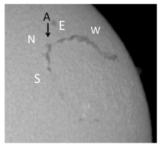
Figure 1: Filament observed on September 20, 2013, with two sections oriented east-west (EW) and north-south (NS) respectively (Meudon spectroheliograph survey). The letter A indicates the junction between the two sections and is clearly a foot of the filament.

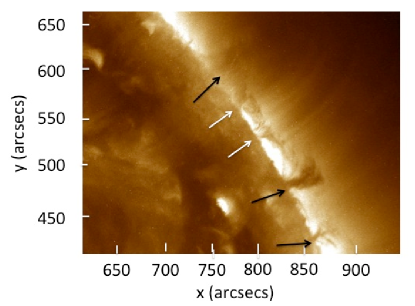
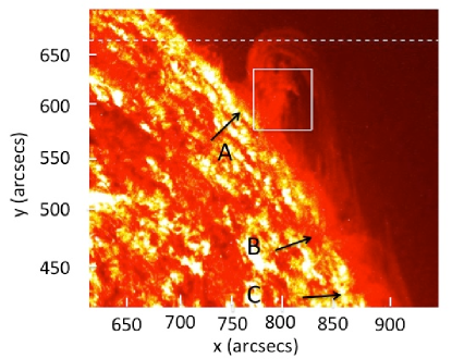
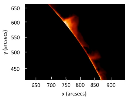
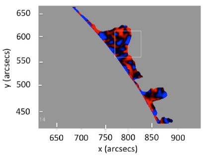
Figure 2: (top panels) Prominence observed on September 24, 2013, at 12:22 UT in 193 Å  (left), and in 304 Å  (right) from SDO/AIA. The black arrows and the letters A, B, C indicate feet of the 304 Å prominence. The white arrows are other feet only present in 193 Å. (bottom panels) The prominence observed in H$\alpha$ by the MSDP (left) intensity, and (right) Doppler shift in H$\alpha$ $\pm$ 0.3 Å  black/white (blue/red on the online version) indicate blueshift/redshift limited to $\pm$ 2 km/s). The boxes in the 304 Å image and in the Doppler shift image are approximately the field of view of the IRIS slit jaws (50 x 50 arcsec).

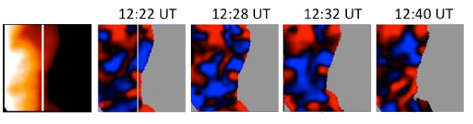
Figure 3: H$\alpha$ intensity image (left) and four Doppler shift images obtained in H$\alpha$ $\pm$ 0.3 Å  (MSDP) (right) in the FOV of IRIS. The Mg II h spectra at the same times are presented in the left panels of Figure 7. Black/white (blue/red on the online version) are the blueshifts/redshifts limited to $\pm$ 2 km/s. The white vertical line approximately represents the location of the IRIS slit 1 used in Figure 6.

2 Observations

2.1 Description

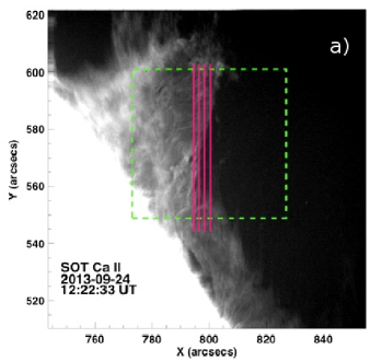
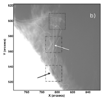
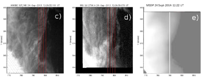
Figure 4: (a) Hinode/SOT Ca II at 12:22 UT with a box representing the field of view of IRIS slit jaw and four vertical red lines, the four IRIS slits, and (b) the same Ca II image overlaid with the contours of the H$\alpha$ intensity of MSDP and three small boxes: the top box indicates a turbulent region, the middle box with the white arrow a small dark bubble, the bottom box with the black arrow a large limb bubble. An online movie of Hinode/SOT Ca II shows the temporal evolution of the image (b); the boxes drawn in (b) help to follow the different dynamics observed in the prominence. (bottom panels) Images obtained with three different instruments in the IRIS field of view ( c) in Ca II (SOT), (d) in Mg II (IRIS slit jaw), and (e) in H$\alpha$ (MSDP).

A long filament with two perpendicular sections (section EW N35^∘-38^∘ and the section between N15^∘ and N30^∘ ) was crossing the limb on September 24, 2013 (Figure 1). The intersection (A) between these two sections was just at the limb on September 24 and corresponds to a filament foot or barb (see the arrow).

The prominence as observed in 304 Å with SDO/AIA consists of a large triangle in the north (x=800 arcsec, y=600 arcsec), which is probably part of the EW section integrated along its axis, and the feet A, integrated along the line of sight, and a bright arch of long horizontal threads parallel to the limb (Figure 2). This long arch is part of the NS section, between pillars or feet (A, B, C, in Figure 2), according to the heliographic coordinates of the filament. Material is continuously flowing along the long threads in both directions. In the 193 Å filter the prominence appears dark due to the absorption of the coronal line by resonance continua of hydrogen and helium at this wavelength. The dark structures in 193 Å  are similar to those in H$\alpha$ because they have similar optical thickness (Anzer & Heinzel, 2005; Schmieder et al., 2004). The shape of the dark absorption is very different from the emission prominence observed in 304 Å (Figure 2). The emission in 304 Å is due to the scattering of chromospheric line radiation and partially due to the presence of a prominence-corona transition region (Labrosse et al., 2010). We want to highlight that the H$\alpha$ prominence (here observed in absorption in the 193 Å coronal line) has more anchorage points (feet) with the photosphere than the 304 Å prominence. It confirmed that lateral extensions in EUV filaments (channels) do not always coincide with H$\alpha$ filament feet or barbs (Aulanier & Schmieder, 2002; Schmieder et al., 2014b).

2.2 MSDP

The Meudon MSDP observations of prominences in H$\alpha$ consist of series of five spectral images 465 arcsec x 60 arcsec with 6 arcsec overlaps in each time sequence. The exposure time is 100ms. Sequences of observations are done during 15 minutes with a 30 sec cadence. They have been processed with the MSDP software. On September 24, ten sequences of observations were done between 12:09UT and 15:09 UT. We focus our study on the sequence starting at 12:22 UT, and 12:38 UT because it is in the interval of the IRIS observations. In each solar point an H$\alpha$ line profile is obtained over a wavelength range of +/- 0.7 Å. Doppler shifts can be computed for any wavelength in this wavelength range with an accuracy of 0.5 km/s (Figures 2 and 3).

2.3 Hinode

The Hinode (Kosugi et al., 2007) SOT (Tsuneta et al., 2008; Suematsu et al., 2008) consists of a 50 cm diffraction-limited Gregorian telescope and a Focal Plane Package including the narrowband filtergraph (NFI), the broadband filtergraph (BFI), the Stokes Spectro-Polarimeter, and Correlation Tracker (CT). For this study, images were taken with a 30 sec cadence in the Ca II H line at 3968.5 Å using the BFI. The Ca II images have a pixel size of 0.109″, with a field of view of 112$\times$ 112″ (Figure 4).

2.4 THEMIS

The THEMIS/MTR instrument (López Ariste et al., 2000) was used to do spectropolarimetry of the He D₃ line in the observed prominence. The spectrograph slit was oriented parallel to the local limb. This direction subsequently defined the sign of the linear polarization: positive Stokes Q means parallel to the slit and, in consequence, parallel to the local limb. The observations were obtained with same setup previously described by Schmieder et al. (2013). The use of a grid mask with segments 15.5 arcsec wide along the slit is required to perform accurate measurements. To speed the record of the full Stokes parameters, the overlap of the segments is minimized. The exposure time is two seconds. Rasters are obtained with steps of 2″ from the limb to the top of the prominence. In our case a field of view, approximately 120″  by 25″ , was covered in approximately two hours. The intensity map of the prominence in He D₃ corresponds reliably to the 304 Å image of SDO/AIA (Figure 5).

2.5 IRIS

IRIS performed a four-step coarse raster observation from 12:14 UT to 15:13 UT on September 24, 2013. The pointing of the telescope is 798 arc sec, 573 arc sec. The spatial pixel size is 0.167 arc sec. The raster cadence of the spectral observation in both the near ultraviolet (NUV 2783 - 2834 Å) and the far ultraviolet (FUV 1332-1348 Å and 1390-1406 Å) wavelength bands was 35 seconds. Exposure times were 8 seconds. Slit-jaw images (SJI) in the broadband filters (2796 Å and 1400 Å ) were taken at a cadence of 18 seconds. The 1400 Å slit jaw is an integration of the FUV emission within a range of about 40 Å (including the total emission of two Si IV lines). The FOV was 6x50 arc sec² for the raster and 50x50 arc sec² for the SJI. The calibrated level 2 data was used in our study. Dark current subtraction, flat field correction, and geometrical correction have been taken into account in the level 2 data (De Pontieu et al., 2014).

We mainly used the Mg II k 2796.4 Å and Mg II h 2803.5 Å lines and the SJI 1400 and 2796 Å data for this study. The Mg II h and k lines are formed at chromospheric temperature (10⁴ K). The SJI 2796 Å  filter samples emission mainly from the Mg II k line, while emission in the 1400 Å  filters from the Si IV 1402 Å and 1393 Å lines formed in the prominence transition region (PCTR). The UV continuum at 1400 Å  formed in the lower chromosphere is not present for a prominence observed at the limb contrary to observations on the disk. The co-alignment between the different optical channels of IRIS was achieved by checking the position of horizontal fiducial lines.

3 Results

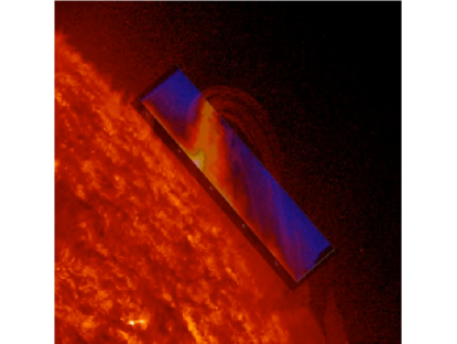
Figure 5: THEMIS image in He D₃ line overlaid on an AIA 304 Å  image. We note the large scale 304 Å  arches with bright loops.

3.1 Co-alignment of the different observations

The co-alignment of the observations obtained by the different instruments is rather difficult, particularly with IRIS. Cross-correlation between the AIA 1600 Å  image and the IRIS SJI images was used for the co-alignment between IRIS and SDO (Figure 2). The co-alignment between SOT and IRIS is done by using the 1600 Å  SDO images and the 2786 IRIS slit jaws. The Ca II and Mg II maps have many similarities (Figure 4). The MSDP maps were aligned with SOT by using the intensity on the disk in the H$\alpha$ and Ca II lines (Figure 4). The THEMIS He D₃ intensity map was co-aligned with AIA images in 304 Å  (Figure 5).

Figure 6: Doppler shifts in the prominence along the IRIS slit 1 in the wide $\lambda$-band in the Mg II k line at 12:22:23 UT (solid line) and in a narrow $\lambda$-band in H$\alpha$ (dashed lines) for two cuts close to the IRIS slit position according to the accuracy of the co-alignment between the MSDP and IRIS. Positive/negative values are red/blueshfits.

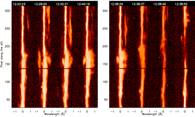
Figure 7: Examples of Mg II k line spectra: evolution of the Mg II 2796.4 Å spectra at 12:22, 12:28, 12:32, 12:40 UT in slit 1 (left). Examples of 2796.4 Å spectra in the four slits of IRIS located from east to west in the slit jaws (slit 1 at 12:38:29, slit 2 at 12:38:37 UT, slit 3 at 12:38:46 UT, slit 4 at 12:38:55 UT) (right), The spectra are between pixel 8 and pixel 314 along the slit. The wavelength range of the Mg II spectra is 2795.00 - 2797.78 Å and the length of the slit is 47 ”. The dark line at pixel=136 is an instrumental feature used for the alignment of the different lines in the spectra. The zero is taken as the velocity reference. North is up. An online movie of the Mg II k spectra is available, see Figure 14 in the Appendix .

3.2 Dynamics of the Ca II prominence

The Ca II line movie (Ca II movie online) reveals turbulent behavior of the plasma in different parts of the prominence (top box in Figure 2 top right panel). It is impossible to follow the evolution of structures. The plasma is fuzzy. This part corresponds to the northern part of the IRIS slits. In the middle of the IRIS slits, the Ca II images show very clearly a small dark bubble (3 arcsec) surrounded by bright rims (middle box in Figure 2 top right panel). It is also visible in the Mg II lines. This bubble corresponds to pixels in the spectra where there is a change in behavior of profiles: from narrow to broad with double peaks. In the bright rims knots go down frequently around 13:00 UT. In the left part on the images we also see oblique threads striating the prominence. These threads exhibit counter streaming. Finally we see the emergence of a bubble (semi-sphere of 20 arcsec of diameter) close to the limb in the right part of the prominence (bottom box in Figure 2 top right panel). Between 12:10 UT and 13:30 UT, the bubble rises to an altitude of 10 arcsec over the limb with a velocity of 2 km/s. It looks similar to the bubbles previously observed with Hinode/SOT by Berger et al. (2011); Dudík et al. (2012). The authors invoked an emerging flux as the cause of such bubbles in a weak bipolar field environment. Thermal instability (Berger et al., 2011) or magnetic pressure excess (Dudík et al., 2012) would lead to the slow rise of bubbles through the prominence. The location of the large bubble in the Hinode FOV is unfortunately outside of the IRIS FOV. No study on the temperature and the density of the bubble can be achieved using the IRIS spectra to resolve the question of the existence of a thermal instability. We suggest that the magnetic solution is acceptable and the dark area in the bubble is the corona that we see under the prominence. Slow rising prominence before eruption is a common observation. Magneto-hydrodynamic models based on the torus instability tell us that a prominence modeled as a flux rope should reach a given threshold height to erupt (Gosain et al., 2012; Török et al., 2009).

3.3 H$\alpha$ profiles

We obtained a map of H$\alpha$ profiles on the whole prominence for each MSDP observation time. From the line profiles, Doppler shifts have been computed by the bisector method for H$\alpha$ +/- 0.3 Å. We focus our study on the time 12:22 UT (Figure 2). The range of the values is between - 3 km/s and 4.5 km/s, consistent with earlier observations of prominences (Labrosse et al., 2010). Large Doppler shifts are only measured at the tops of prominences where only a few threads are integrated along the line of sight (Schmieder et al., 2010). High velocity threads in H$\alpha$ larger than 20 km/s cannot be detected in these observations because the H$\alpha$ wavelength band of the MSDP is too narrow. The evolution of the Doppler shift pattern is relatively fast (Figure 3).

We present in Figure 6 the cuts of the H$\alpha$ Doppler shifts along the slit 1 of IRIS FOV at 12:22:23UT (two possible positions according to the accuracy of the co-alignment). The intensity of the H$\alpha$ line along the slits 2, 3, and 4 is under the threshold of the intensity where Dopplershifts can be computed. The Doppler shift structures have a size on the order of 18 arcsec. The H$\alpha$ Doppler shift values are lower than those of the Mg II lines, which can be explained by the lower spatial resolution of the MSDP and by the fact that the H$\alpha$ line has lower optical depth so that the observations integrate more structures along the line of sight (LOS). The seeing also smooths the values.

Table 1: Characteristic parameters of the Mg II line profiles observed by IRIS (observation) and copied in Paletou et al. (1993) (model).

parameter	unit	Observation	(IRIS)	Model of	Paletou et al. (1993)
		Mg II h	Mg II k	Mg II h	Mg II k
FHWM	Å	0.15	0.16	0.40	0.40
Central intensity	10-7 erg s-1 cm-2 sr-1 Hz-1	2-2.4	2.3-3.1	1- 4	1- 4.3
Integrated intensity	104 erg s-1 cm-2 sr-1	1.2-2.6	1.8-3.7	2.4	3.7

Table 2: Several components of Mg II line profiles at 12:28 UT and at 12:38 UT for some pixels along the slit (Dopplershift velocity in km/s).

pixel number	peak1	peak2	peak3	peak4	peak5
140	-64.2		-4.1	24.5
150	-67.0	-29.0	0.6	25.5	75.6
160	-63.8		-1.1	20.6	67.5
200			-1.5
250			0.4		62.9
300			2.3	42.4	65.1
100			-5.0	15.5
164	-41.9	-22.7	2.8	32.8	72.1
270			0.7		71.5

Figure 8: IRIS line profiles of Mg II 2796.4 Å: (first and second rows) at 12:28:20 UT for six pixels along the slit (140, 150, 160, 200, 250, 300); (third row) at 12:38:29 UT for y=100, 164, and 270 (see spectra in Figure 7). We note that lateral peaks (indicated by ticks) are resolved on both sides of the main peak indicating fine structures along the LOS with Doppler shifts reaching 60 to 80 km/s (see Table II).

Figure 9: Characteristics of the Mg II k 2796 Å (solid line) and Mg II h 2803 Å  (dashed line) along the IRIS slit 1 at 12:22:23 UT: full half width maximum (FHWM), integrated intensity (I-int), Dopplershifts (velocity), and peak intensity (I-peak) assuming Gaussian profiles. The ratio of the peak intensity between the two lines is equal to 1.24.

3.4 Mg II profiles

The IRIS profiles are very interesting. In the northern part of the slits the profiles are very narrow; in the southern part the profiles have secondary peaks (Figs 7 and 8, IRIS movie online). The spectra correspond to pixels between 8 and 314 along the slit in the slit jaws with a pixel size of 0.167 arcsec. Horizontal dark lanes are the horizontal fiducial lines used for co-alignment between the different wavelengths. Slit 4 corresponds to the extreme west edge of the triangle-shaped prominence in the slit jaw and is frequently empty of signal or with a long gap of very weak signal. We focus our study mainly on slit 1 located at the east in the slit jaw where the signal is the strongest. The dispersion per pixel $\Delta\lambda$ is equal to 0.02546 Å  and $\lambda_{0}$=55.47 pixel is the centroid of the averaged line used as the rest wavelength. The most of the profiles of the Mg II lines are not reversed and the maximum peak intensity is around 3 x 10^-7 erg s^-1 sr^-1 cm^-2 Hz^-1 (Table I). The FHWM of the Mg II lines is around 0.15 Å. If we fit the whole profile with a single Gaussian including the different peaks we obtained a FHWM of 0.4 Å. This is what can be seen with a spectrograph with low spectral resolution (Vial, 1982).

We compare the observed profiles with the theoretical Mg II line profiles computed with non-LTE radiative transfer models in a 2D static slab (Paletou et al., 1993) (Table I). For low peak intensities (lower than 2 x 10^-7 erg s^-1 sr^-1 cm^-2 Hz^-1) both the computed profiles and the observed ones are not reversed. For higher intensities the computed profiles are always reversed. This is not the case with our observations. When the observed profiles are wider, we find that there are two structures: one is nearly static and the other one has a velocity on the order of 20 km/s (Table II). Only a few line profiles are reversed. We consider reversed profiles when the two peak wavelength positions are more or less symmetric with respect to the line center (for example, in Table II at y=100 at 12:38 UT and perhaps y=160 at 12:28 UT, but the peak positions are not symmetric there). The distance between the two peaks in the case of reversed profiles is around 0.2 Å. The ratio between the maximum intensity of the two Mg II lines (k/h) is around 1.24; between the integrated intensity it is 1.33, the FHMW maximum ratio is similar (1.1), and the Doppler shifts are equivalent (Figure 9).

The predicted computed profiles do not fit the observations in many respects. Similar surprising results were found when we observed the hydrogen Lyman line series in prominences. Some prominences presented profiles that were not systematically reversed (Heinzel et al., 2005; Schmieder et al., 2007; Gunár et al., 2007; Curdt et al., 2010; Schwartz et al., 2012). This has been discussed in terms of the orientation of the magnetic structures in prominences and the column mass.

The narrow profiles in the northern part of the slit correspond to small Doppler shifts ($\pm$ 5 km/s). This part is in the section of the prominence plasma that looks turbulent in the Ca II movie. For unresolved turbulent plasma, the profiles should be broaden. This is not the case. The secondary weak peaks of the profiles are wider and have a long extension along the slit (e.g., at 12:32:32 UT in Figure 7). They could correspond to small scale turbulence, but these peaks are mainly redshifted and not symmetric versus the line center as we expect for unresolved turbulence. The global structure with turbulence plasma would be globally redshifted in that case.

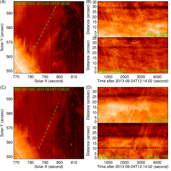
Figure 10: (left panels) (A) and (C ) Si IV slit jaws (47” $\times$ 47” ) respectively at 12:38:28 UT and 13:00:32UT showing the cuts of the time slice when the flows are crossing the IRIS slits. (right panels) The time slice diagrams are presented in pairs corresponding to MgII and Si IV slit jaws for each cut. (B) corresponds to the cut in (A), (D) to the cut in ( C). The time slice diagrams show parallel straight lines indicating flows going towards the southeast/northwest direction with a projected speed respectively of 52.5 and 33.6 km/s. (a Si IV slit-jaw movie is available in the online version with Figure 14 in the Appendix explaining the movie. )

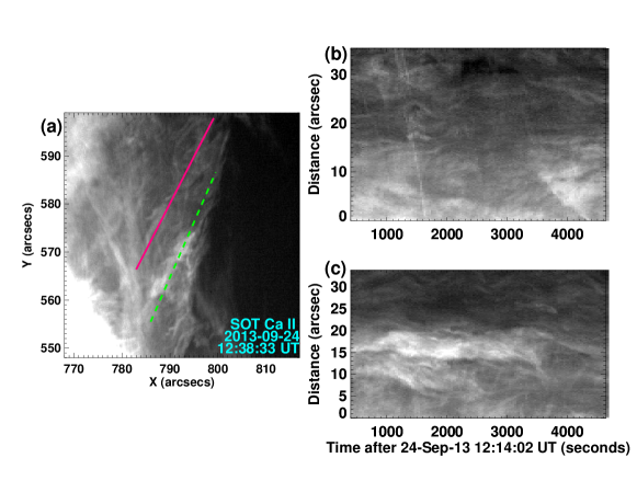
Figure 11: (a) Ca II image showing the two cuts used to make the time slice diagrams presented in ( c) and (d). The time slice diagram in ( c) shows parallel straight lines indicating flows going towards the southeast/northwest direction; in (d) we see mainly a quasi static component and very weak straight lines.

3.5 Mg II Doppler shifts

Doppler shifts are computed using single or multi-gaussian fits to the peaks of Mg II line profiles. The Mg II Doppler shifts computed with single fit are comparable to the H$\alpha$ Doppler shifts. We show an example of such a comparison for 12:22 UT (Figure 6). The Doppler shift/intensity pattern in the Mg II h and k lines has a periodicity of about 5 arcsec in width with smaller structures (1.6 arc sec) along the slit. The H$\alpha$ Doppler structures have a triple size. The structures are clearer in Mg II lines because the higher optical depth of the line than in H$\alpha$ (Heinzel, private communication).

In the northern part of the slits, the profiles are narrow and usually one Gaussian profile fits the observations well. In the southern part, fine structures in the Mg II lines are observed in the profiles (Figure 7). The spectra along the slit (at 12:28 UT and at 12:38 UT, for example) show many different structures along the LOS (Figure 8). We used multicomponent Gaussian fits to compute the Doppler shifts of each individual thread crossing by the LOS (Table II). A relatively static component is always present, exhibiting the highest peak (peak 3). High Doppler shifts of up to 70 - 80 km/s are detected. In some pixels (y=160), we note the structures with opposite Doppler shifts suggesting that counter streaming flows are present in the prominence (Zirker et al., 1998).

We have to mention that here we use the centroid of the Mg II line profiles averaged over the whole region as the rest wavelength, since neutral lines cannot be used in prominence observations to absolutely calibrate the wavelength. Nevertheless there are no neutral lines in the present observed wavelength range. In addition it has been found that the orbital variation of neutral line positions in other IRIS observations is usually less than 5 km/s peak to peak. So here we estimate an uncertainty of about 5 km/s for the velocity determinations (References in IRIS technical note 20-ITN 20 Wavelength Calibration- http://iris.lmsal.com/documents.html). This means that regarding the 5 km/s velocity as stationary is reasonable.

3.6 Transverse flows measured in Mg II and Si IV slit jaws

With a time slice procedure, we computed the transverse velocity field in some moving structures using the slit-jaw images (Figure 10). In the movies (online) of the slit jaws, the global structure changes slowly. However, fine threads exhibiting fast moving material cross the slit. For example, in pixels around y= 300 material goes towards the limb between 12:29 UT and 12:39 UT, and for pixels in the middle of the raster material goes to the north between 12:56 UT and 13:02 UT (Figure 10). The projected speeds of these features on the plane of the sky, computed from the time slices are respectively 52 km/s and 33 km/s.

The measured speeds are the same for the two slit-jaw sets (SJI 1400 and SJI 2796). These transverse velocities correspond to knots following threads that cross the IRIS slit around 12:38 UT and 13:01 UT. The transverse velocities correspond to high Doppler shifts detected in the structures crossing the slit. This indicates that the fine threads moving at the front of the prominence are oriented at a given angle with respect to the plane of the sky. For the knot crossing the slit at 12:38 UT the angle of the thread is around 50 degrees with the plane of the sky. The velocity vector strength may reach up to 100 km/s. These fine threads could be fine threads along the spine of the prominence between A and B, or between A and C (N-S filament in Figures 1 and 2).

We performed a similar analysis with Ca II images and compare it with IRIS time slice (Figure 11). The brightest pattern with no significant motions is similar in Ca II and in Mg II. It could be interpreted as corresponding to the quasi-stationary plasma. There is also an analogy between the fine threads crossing the slit, but it is not clear if these are exactly the same threads or parallel threads.

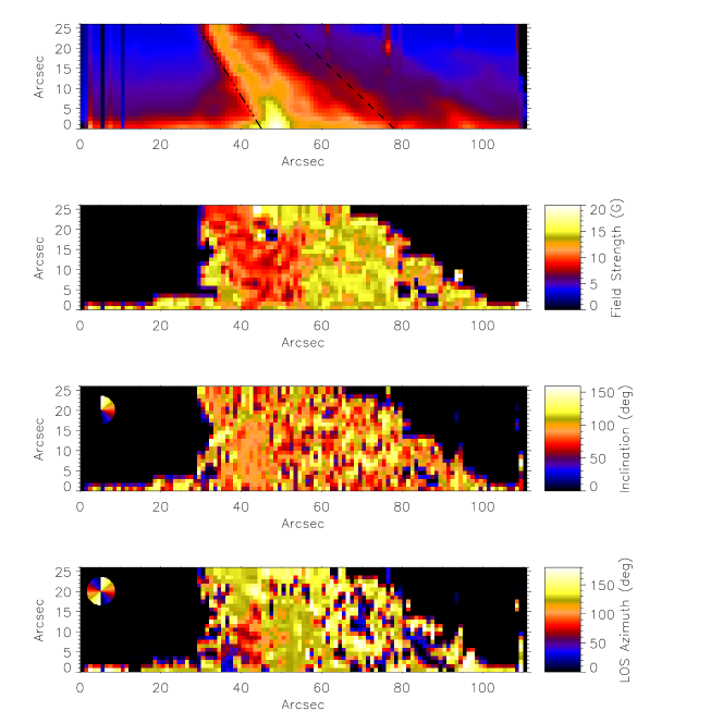
Figure 12: THEMIS observation on September 24, 2013, obtained between 12:24 UT and 14:30 UT: (from top to bottom) intensity, magnetic field strength, inclination, and azimuth. The two lines (dot-dashed and dashed) in the intensity image represent the location of the two cuts used in Figure 13. The origin of the cut in the brightest region is at x=40, y=0; the origin of the IRIS slit is at x-80, y=0.

3.7 Magnetic field vector: macroscopic component

The raw data of the THEMIS/MTR mode was reduced with the DeepStokes procedure (López Ariste et al., 2009) and the Stokes profiles were fed to an inversion code based on Principal Component Analysis (López Ariste & Casini, 2002; Casini et al., 2003). Initially, the observed profiles were compared against those in a database generated with known models of the polarization profiles of the He D3 taking into account the Hanle and Zeeman effects (López Ariste & Casini, 2002). The details of the MTR data reduction are completely explained in Schmieder et al. (2013). The most similar profile of the data base containing 90000 profiles is kept as the solution and the parameters of the model used in its computation are kept as the inferred vector magnetic field height above the photosphere and scattering angle. Error bars are determined for those parameters as well by doing statistics on all other models which are sufficiently similar to the observed ones, although not as similar as the one selected as the solution.

Figure 12 presents the maps obtained after inversion of the Stokes parameters recorded in the He D₃ line: (a) intensity, (b) magnetic field strength (c) inclination, (d) azimuth. The angle origin of inclination is the local vertical, the origin of the azimuth is the LOS in a plane containing the LOS and the local vertical. We see that the brightest parts of the prominence have a mean inclination of 90^∘ which means that the magnetic field in the brightest oblique structure is clearly horizontal. However, there is a large dispersion of the values (+/-30 degrees) from one pixel to the next in the lateral parts of the prominence.

Figure 13 presents the variation of magnetic field strength, inclination, and azimuth along the slit positions of IRIS in Figure 5. The field strength is in the range 5-15 Gauss and mainly horizontal. The inclination is around 90 ^∘ +/-30^∘. The azimuth is close to 90^∘ and again with a large dispersion (+/- 50 degrees). This means that the magnetic field vector is mainly perpendicular to the plane of the sky with a large dispersion of values.

The brightest part of the prominence where the magnetic field is directed horizontally with respect to the solar surface is located mainly in foot A at the intersection of the two sections of the filament (Figure 1). This confirms previous results (Bommier & Leroy, 1998; Casini et al., 2003). Prominence feet observed on the disk have also shown that the field lines are tangent to the photosphere (López Ariste et al., 2006; Schmieder et al., 2013). Their shapes have been reliably represented by linear force free field extrapolations (Aulanier & Démoulin, 1998; Dudík et al., 2008, 2012). The dispersion of the values of the inclination and the azimuth could be due to the foreground transient structures of the large arch seen in 304 Å  (Figure 5).

Figure 13: Variation of the magnetic field, strength, the inclination, and the azimuth (THEMIS): (top panels) data along the IRIS slit, (bottom panels) data along the bright structure.

3.8 Magnetic field: turbulent component

The model used for inversion, and whose results we have just discussed, assumes a unique magnetic field vector per pixel. The low signal-to-noise ratio of the polarization signature advise against assuming more complex scenarios. This single value of the magnetic field vector can be seen as the large scale magnetic structure supporting the prominence and revealed by polarimetry at low spatial resolutions. In the previous subsections we have listed a compilation of observations from IRIS and Hinode SOT with high cadence and high spatial resolution that suggest a more complex magnetic scenario where the local magnetic structure departs from the stand-alone macroscopic horizontal field.

Intrigued by the possibility of unveiling a more dynamic and complex field structure in the prominence we explored the effects of a turbulent field added to a macroscopic field into the Stokes profiles of the He D₃ line. We should say that the word turbulence is used incorrectly here. It may mean actual turbulence in the sense of hydrodynamics, but it may well just mean several unresolved (in time, space, and along the line of sight) magnetic components that are added together in the same pixel of our data set. The polarization of the He D₃ line in the presence of an isotropic field with a strength of roughly 15 G can be readily computed and, to a good precision, results in the absence of Stokes U and V profiles, while every transition involved in the line formation is polarized in Stokes Q to $\frac{1}{5}$ of the polarization at zero field (Landi Degl’Innocenti, 1984). The absence of Stokes U and V profiles in a turbulent field already excludes this possibility from our observations: we do see Stokes U and V signals. If there is a turbulent field at all, it is mixed with a macroscopic average field. Therefore, the single profile in Stokes Q emitted by the turbulent magnetic component was added to the profiles from the macroscopic magnetic component weighted by a filling factor. These new profiles made of the addition of the two components were inverted with the same model of the observed data. The solutions found have systematically smaller field strengths and the inclination is on average the same, but the error bars grow enormously. This growth in the error bars of the inclination is exactly what is observed in the region sampled by the IRIS slit. The spectropolarimetry of the D₃ line would therefore be consistent with a turbulent component as suggested by the other observables cited above and added to a macroscopic field. The field strength in Fig. 13 (top panels) would be just a lower limit to both the macroscopic and the turbulent components, while the inclination of the macroscopic component would still be horizontal. On the other hand, those parts of the prominence with small error bars in the inclination, like those in the bottom panels in Fig. 13 across the brightest parts of the prominence, would not accept a turbulent component but just one single macroscopic field. In this picture the prominence would be made of an organized horizontal and relatively weak field supporting the densest cores of the plasma plus some other regions with stronger horizontal fields in addition to a turbulent field responsible for most of the rapid dynamics of the plasma.

4 Discussion and conclusion

A large quiescent prominence on the northwest limb was the target of coordinated observations on September 24, 2013. Observed on the disk a few days before, we note that the filament consisted of two sections: one oriented east-west and one oriented north-south. The multiwavelength observations of this prominence obtained with the new spectrograph IRIS, Hinode/SOT, SDO/AIA, and from the ground (THEMIS in Canary Islands and the MSDP spectrograph on the Meudon solar tower) were analyzed. The small field instruments (109 arcsec $\times$109 arcsec for the Hinode/SOT, 50 arcsec $\times$ 50 sec sec for IRIS) were focused on the junction of the two sections: the foot A and the integration of the EW filament section. The prominence is shaped like a triangle. The AIA and the MSDP with their large fields of view also show the section NS with different arches and feet. We note the different aspects of the triangle-shaped prominence observed in He lines (304 Å  and D₃) and in the chromospheric lines (CaII and H$\alpha$, Mg II). This results from the different temperatures of formation of the lines but also of their different optical thickness.

The principal results concern the dynamics and the magnetic field measured in this triangle. The spectro-polarimetry of the prominence indicates that the magnetic field is mainly horizontal all over the observed region with a field strength of only 5 to 15 Gauss. This confirms the previous magnetic modeling of filaments using linear or nonlinear force free field extrapolation showing that prominence material is sustained in shallow dips of field lines even in the barb or feet of the filament (Aulanier & Démoulin, 1998; Aulanier & Schmieder, 2002; van Ballegooijen, 2004; Dudík et al., 2008). The aspect of apparent vertical structures could be just a perspective view of the dips as showed the simulation of Dudík et al. (2012) inserting parasitic polarities in a shear bipolar region to create a filament. The analysis of a different prominence by THEMIS had recently clearly shown the horizontal dips in the feet of the prominence (Schmieder et al., 2013).

Such a stable magnetic field is somehow disturbed by the dynamics of the observed plasma. First, the observations in the Ca II movie revealed a complex tangling of dynamical structures in the prominence. This aspect gives a priori the same impression as the tangled model for prominence proposed by van Ballegooijen & Cranmer (2010). We detect some relatively stable background emission while some threads in the front have material flowing rapidly. This was also visible in the IRIS slit-jaw movies. The transverse velocities of the fast moving features along the oblique threads crossing the IRIS slits were obtained with a time-slice analysis. The features or blobs were running with velocity up to 50 km/s. In one part of the Ca II images and in both of the IRIS slit jaws we see some disorganized motions, which could be interpreted as MHD turbulence.

We explored the possibility of a departure of the magnetic field from the average horizontal field retrieved by our inversions. We excluded a fully turbulent field since it would result in null Stokes U signatures contrary to the observations. However a model made of a horizontal macroscopic field plus a turbulent component would be interpreted by our inversion codes as a horizontal field with large error bars and smaller field strength. This is compatible with our observations in the most dynamic parts of the prominences, those observed with IRIS. Our conclusion draws a picture of the prominence where an organized horizontal and relatively weak field supports the densest cores of the plasma while some other regions with stronger horizontal fields in addition to a turbulent field would be responsible for most of the rapid dynamics of the plasma.

These rapid dynamics of the plasma was seen at its best in the IRIS spectra of the Mg II lines. The Mg II spectra exhibit multiple structures along the line of sight. The profiles of the lines have a Gaussian profile with weak intensities and are not reversed profiles contrary to the predicted theoretical profiles (Paletou et al., 1993). We compute the Doppler shifts and found discrete values from a quasi-static component ($\pm 5$ km/s similar to the H$\alpha$ Doppler shifts) to 60- 70 km/s. The high Doppler shifts correspond to the large transverse motions measured along the oblique threads crossing the slits obtained with a time-slice analysis. In some pixels high positive and negative flows are detected suggesting structures with opposite Doppler shifts crossing the line of sight. These structures have an angle with the plane of the sky of about 45 degrees, and their real velocity may reach 100 km/s. Spectroscopy is a powerful diagnostics tool to detect the real orientation of the structures and the real velocities.

These oblique threads may be found along the field lines in the large arches observed in 304 Å. Is it fast moving cool material due to fast cooling of EUV plasma? There is counter streaming along these features. It has been suggested that counter streaming could occur because of longitudinal oscillations (Chen et al., 2014; Luna et al., 2014). The material in the dips could travel on one side or the other side. For large scale structures the siphon flow mechanism could be more important than the counter streaming leading to large flows towards one end of the prominence or the other end. The siphon flow may go from the more magnetized end to the lower magnetized end (Chen et al., 2014). In our case the bright arches could be considered as a large structures containing siphon flows.

How can we reconcile two magneto-hydrodynamic systems, one mainly horizontal and one turbulent? This question was also put forward by Priest (2014). It should be important to work on the interpretation of the Stokes parameters profiles in this framework. The first test presented in this work is encouraging; while with the present data one cannot invert more complex magnetic models, we can at least propose models compatible with both the polarimetric and the imaging observations.

Finally, IRIS reveals the complexity of MgII line profiles in an otherwise quiescent prominence (the filament was quiescent with no network environment). Even when we consider emission profiles having only one peak, it is difficult to interpret them in terms of the existing models (Paletou et al., 1993) because these models show mostly reversed profiles. Other observed profiles exhibit a multipeak structure, which we interpret as due to the line-of-sight Doppler shifts of individual emission profiles. In a future paper we plan to perform a detailed quantitative analysis of both types of MgII profiles, using the existing non-LTE codes. Moreover, the future modeling should consistently explain the emission in the H$\alpha$ line which we also present in this paper; H$\alpha$ can thus provide an important constraint on the modeling of MgII lines.

Appendix

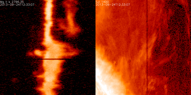
Figure 14: Figure online explaining the IRIS movies: (left side) Mg II k line spectra, (right side) IRIS Si IV slit-jaw image, the vertical line is the slit position of the spectra. The wavelength range of the Mg II spectra is 2795.00 - 2797.78 Å. The FOV of the Si IV slit-jaw image is 47”x47”.