How molecular knots can pass through each other

Abstract

We propose a mechanism in which two molecular knots pass through each other and swap positions along a polymer strand. Associated free energy barriers in our simulations only amount to a few $k_{B}T$, which may enable the interchange of knots on a single DNA strand.

Ever since Kelvin conjectured atoms to be composed of knots in the ether 1 , knots have stimulated the imagination of natural scientists and mathematicians alike. In recent years the field went through a renaissance and progressed considerably, spurred by the realization that topology may not only diversify structure, but can also have a profound impact on the function of biological macromolecules. Knots in proteins have been reported 2 ; 3 ; 4 ; 5 ; 6 ; 33 ; 7 and even created artificially 8 . Topoisomerases can remove 9 or create 10 knots in DNA, which may otherwise inhibit transcription and replication, and viral DNA is known to be highly knotted in the capsid 11 ; 12 ; 13 ; 14 ; 15 . Artificial knots have also been tied in single DNA molecules with optical tweezers and dynamics have been studied both experimentally and with computer simulations 16 ; 17 . Knots are also known to weaken strands, which tend to rupture at the entrance to the knot 32 ; 34 . Even though most of these examples are not knotted in a strict mathematical sense 18 , which only defines knots in closed curves, they nevertheless raise fundamental questions and challenge our understanding of topics as diverse as DNA ejection 19 and protein folding 20 . Knots may also play a role in future technological applications, particularly in the advent of DNA nanopore sequencing 21 . While the probability of observing a knot in a DNA strand of 10 kilo base pairs in good solvent conditions only amounts to a few percent 22 ; 23 , knots and even multiple knots will become abundant once strand sizes exceed $100000$ base pairs in the near future. Part of this problem was recently addressed in a simulation study 24 : a single knot will not necessarily jam the channel once it arrives at the pore, but may slide along its entrance.

In the following we would like to elucidate a fascinating and little-known property of composite knots: Two knots can diffuse through each other. In our simulations we employ a standard bead-spring polymer model 25 , which does not allow for bond crossings if local dynamics are applied. Furthermore we apply an additional angular potential and tune the stiffness of the chain such that in good solvent (high salt) conditions the persistence length of DNA is reproduced (for $\kappa=20k_{B}T$). Our polymer consists of $250$ monomers which corresponds to roughly $1875$ base pairs. Details on our coarse-grained model, the mapping onto DNA and determination of knot sizes are given in Materials and Methods section. Note that no bias was applied so that our simulations are solely driven by thermal fluctuations. As Supporting Information a video of one “tunneling” event is provided (Video IV).

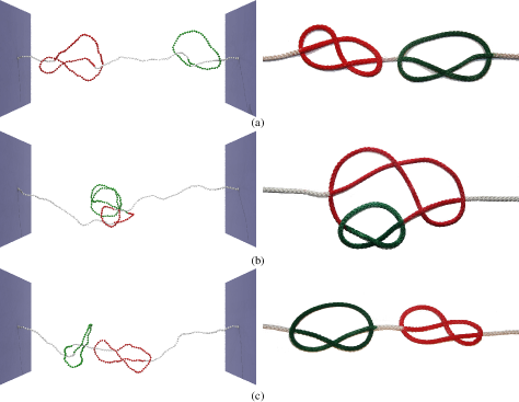
Figure 1: Left: Snapshot pictures taken before (a), while (b) and after (c) $3_{1}$ (green) and the $4_{1}$ (red) knots interchange positions along the strand. Right: Simplified representation.

In FIG. 1 we have prepared a starting configuration with a trefoil knot ($3_{1}$) on the right hand side (green), which is characterized by three non-reducible crossings in a projection onto a plane, and a figure-eight knot ($4_{1}$) on the left (red), which has four crossings. Both termini are connected to a repulsive wall on each side. The distance between walls was chosen to correspond to the typical end-to-end distance ($R_{ee}$) of an unentangled polymer strand of this size ($d\approx 88\sigma$). Simulations take place in the NVT ensemble (Langevin thermostat) using the CPU version of the HOOMD package 26 . Knots are identified using an implementation of the Alexander polynomial as described in 27 . The location and the size of each knot is determined by successively deleting monomers from both ends 28 until we detect first the trefoil or the figure-eight knot and finally the unknot or vice-versa. The arithmetic mean of the starting and the end monomer of the knot is called its “center”.

I Results

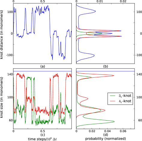
Figure 2: (a) Distance between the respective “knot centers” as a function of simulation time. The positions around $+100$ correspond to configurations in which the two knots are separated. At $-100$ the knots are also separated, but positions along the strand are interchanged. The transition region in which the knots are entangled and pass through each other is located around $0$. (b) Corresponding probability profile (blue) obtained from (a). Interestingly a triple peak forms in the intertwined state. Simulations in which the $4_{1}$ knot passes through the enlarged $3_{1}$ knot only contribute a single peak (green), while for the opposite situation two peaks arise (red). (c) “Size” of the trefoil (green) and the figure-eight knot (red) as a function of simulation time. The same section was chosen as in (a). “Swapping events” and attempted events are accompanied by a considerable enlargement of one of the two knots to around the combined equilibrium size of both knots (blue line), while the other knot which diffuses along the big knot only grows a bit. (d) Corresponding probability profile obtained from (c). The data shown in (a) and (c) is smoothed by applying a running average. For details and implications see Materials and Methods. FIG. S1 also shows the raw data.

In FIG. 2a we follow the location of the knot centers with respect to each other, and record their distance (in units of monomers) as a function of simulation time. In this framework, the two knots are separated when the two centers are around $100$ monomers apart. At $-100$ the knots are also separated, but positions along the strand are interchanged. Knots are intertwined when centers coincide. As shown in FIG. 2a knots may pass through each other over and over again via an entangled intermediate state. Can we understand this peculiar diffusion mechanism? In FIG. 2c (which shows the same section as in FIG. 2a) we record the size of each knot. When two knots are separated the trefoil knot occupies around $60$ monomers, whereas the figure-eight knot is slightly larger at around $80$ monomers. In the entangled intermediate state one of the knots suddenly expands to a bit less than the combined size of the two knots in the separated state, whereas the size of the other knot grows only marginally. Intriguingly, it is not always the larger figure-eight knot which expands even though its expansion is a bit more likely as can be seen in the accumulated histogram in FIG. 2d. As the two knot centers more or less coincide in the entangled state we conclude that the smaller knot diffuses along the strand of the enlarged knot (as depicted in FIG. 1b) until the two are separated again. They may then either occupy the same positions as before or have interchanged positions along the strand. At large stiffness, the probability distribution of the intertwined state is split up into a triple peak (FIG. 2b) which emerges from two separate contributions. If the $4_{1}$ knot passes through the enlarged $3_{1}$ knot there is only a single peak in the middle (green curve). Vice versa, two slightly shifted peaks arise (red curve) due to the symmetry of the enlarged $4_{1}$ knot (compare with FIG. 1b).

I.1 Topological free energy

We can also derive an estimate for the “topological” free energy barrier which needs to be overcome in a “knot swapping” event. This barrier essentially accounts for the obstruction caused by entanglements. In FIG. 2b we have accumulated data from simulations as shown in FIG. 2a to obtain a histogram of the time series and a corresponding probability distribution. For $\kappa=20k_{B}T$ the most likely state is the combined state whereas the separated states are metastable.

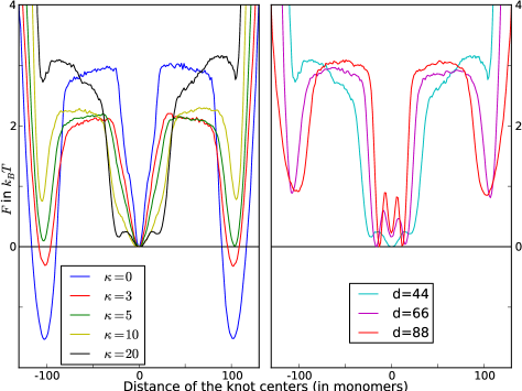
Figure 3: (a) Free energy profiles derived from probability distributions as shown in FIG. 2b. The curves correspond to simulations in which the stiffness of the chain was modified at a constant wall distance ($d\approx 44\sigma$) to apply more or less tension to the string. While the separated states are stable for a flexible chain (blue) the intermediate state becomes stable and more likely at higher stiffnesses (green and yellow). The barrier in the free energy is also reduced by a higher chain stiffness. Note that smaller values for $\kappa$ can also be mapped onto DNA and correspond to larger DNA strands in physiological and lower salt conditions as detailed in the Materials and Methods section. (b) Free energy profiles derived from probability distributions as shown in FIG. 2b. The three curves correspond to three simulations in which the separation of the walls was modified to apply more or less tension to the string while the same angular stiffness ($\kappa=20k_{B}T$) was used. For all wall distances the intertwined state is the most likely state. Note that a pronounced triple peak only emerges for large stiffnesses.

From FIG. 2b the “topological” free energy is derived as $F=-k_{B}T\ln(P)$. When the separated states are stable (as for flexible chains with $\kappa=0k_{B}T$ in FIG. 3a) the system first needs to overcome a barrier ${\Delta F_{1}=-k_{B}T}\cdot\allowbreak\ln(P(\text{entrance to intertwined state})/P(\text{separated state}))$ to reach the metastable intertwined state. Then a second barrier ${\Delta F_{2}=-k_{B}T}\cdot\ln(\allowbreak P(\text{entrance to intertwined state})\allowbreak/\allowbreak P(\text{intertwined state}))$ needs to be overcome to finally swap positions or go back to the original state. If the intertwined state is stable (as in $\kappa=20k_{B}T$ in FIG. 3b) the system needs to overcome $\Delta F_{2}$ to escape into the metastable separated state. In all cases the barriers only amount to $2-5~{}k_{B}T$, which would be accessible in experiments. Can we alter this barrier? FIG. 3a shows free energy profiles from simulations with different angular stiffness at the same wall distance. While in the case of the lowest stiffness the separated states are more likely, the intertwined state is more probable at larger stiffnesses as indicated above. FIG. 3b also shows free energy profiles from simulations in which the walls were placed closer together (to $0.5R_{ee}$ and $0.75R_{ee}$). While the free energy barrier decreases only slightly for $0.75R_{ee}$, the separated states nearly vanish when the two knots are pushed together by the smaller distance of the walls (at $0.5R_{ee}$).

II Discussion and Conclusion

In conclusion, we present a mechanism which allows for two molecular knots to diffuse through each other and swap positions along a strand. The corresponding free energy barrier in our simulations only amounts to a few $k_{B}T$ and should be attainable in experiments similar to 16 (with loose composite knots) and potentially in vivo. The barrier can be altered by changing the chain stiffness as well as the wall distance to make the “tunneling” event more or less probable. To which extent this peculiar diffusion mechanism might affect DNA behavior in nano-manipulation experiments will be investigated in future studies.

III Materials and Methods

III.1 Model and simulation details

The model we apply is essentially a discrete variant of the well-known worm-like chain model (with excluded volume interactions) which has been used extensively to characterize mechanical properties of DNA 22 ; 23 ; 30 ; 31 . We start with a standard bead-spring polymer model from reference 25 which does not allow for bond crossings. All beads interact via a cut and shifted Lennard-Jones potential (eq. 3). Adjacent monomers interact via the finitely extensible nonlinear elastic (FENE) potential (eq. 6). Chain stiffness is implemented via a bond angle potential (eq. 7), where angle $\theta_{i}$ is measured between the beads $i-1$, $i$ and $i+1$. For the interaction with the wall we also apply the repulsive part of the Lennard-Jones potential (eq. 10), where $d_{i}$ is the orthogonal distance from the respective wall to bead $i$. For simplicity we define the normal vector of the walls to coincide with the x-axis of our system.

$$U_{\text{WCA}}(r_{ij}) =\left\{\begin{array}[]{l l}4\epsilon\left[(\sigma/r_{ij})^{12}-(\sigma/r_{ij})^{6}\right]+\epsilon,&r_{ij}\leq 2^{1/6}\sigma\\ 0,&r_{ij}>2^{1/6}\sigma\end{array}\right.$$ (3)

$$U_{\text{fene}}(r_{ij}) =\left\{\begin{array}[]{l l}-0.5kR_{0}^{2}\ln\left[1-(r_{ij}/R_{0})^{2}\right],&r_{ij}<R_{0}\\ \infty,&r_{ij}\geq R_{0}\end{array}\right.$$ (6)

$$U_{\text{angle}}(\theta_{i}) =\quad~{}\frac{1}{2}~{}\kappa~{}(\theta_{i}-\pi)^{2}$$ (7)

$$U_{\text{wall}}(d_{i}) =\left\{\begin{array}[]{l l}4\epsilon\left[(\sigma/d_{i})^{12}-(\sigma/d_{i})^{6}\right],&d_{i}\leq 2^{1/6}\sigma\\ 0,&d_{i}>2^{1/6}\sigma\end{array}\right.,$$ (10)

with $\epsilon=1k_{B}T$, $k=30\ \epsilon/\sigma^{2}$ and $R_{0}=1.5\ \sigma$. The two end beads are grafted to the walls and have the same y and z coordinates. The simulations are run with the CPU version of HOOMD 26 and use the implemented Langevin dynamics thermostat at $T=1$ and $\gamma=1$. All simulations take place in a regime where differences of the strain energies along the knots can be measured but are far away from breaking bonds as seen in 32 ; 34 . We use a time step of $\Delta t=0{.}01$ 25 and evaluate the data each $10^{5}$ MD-steps. Each simulation ran for $4\cdot 10^{9}$ MD steps and each parameter set was simulated in at least $66$ independent simulations. For $\kappa=10k_{B}T$, $d=44\sigma$, e.g., we have performed 131 independent simulations and observed 973 successful swapping events.

III.2 Mapping onto DNA

In the context of knots a similar model was applied in 22 where the parameters were obtained from mapping the probability for obtaining trefoil knots in the polymer model onto the experimental probability observed for a DNA strand of $11.6$ kilo bases as a function of NaCl concentration. Our model (which is based on this model) has essentially two parameters, which can be fitted to mimic real DNA: The chain stiffness $\kappa$ and the diameter of the chain ($\sigma$ in Lennard-Jones units). $\sigma$ is taken from 22 . For high salt concentration ($1$ M NaCl), the effective diameter of the chain is slightly larger then the locus of DNA ($\sigma=2.5\text{nm}$). In physiological salt conditions ($0.15$ M NaCl) the effective diameter (according to 22 ) is somewhat larger ($\sigma=5\text{nm}$). For all salt conditions we assume a persistence length $l_{p}$ of $50\text{nm}$ or $150$ base pairs.

The relevant energy scale of our model is defined by $\kappa$ in eq. 7. For the discrete worm-like chain model

$$\kappa\approx\frac{l_{p}k_{B}T}{\sigma}\quad.$$ (11)

As our model features excluded volume interactions, variable bond lengths and angles, we have verified this relation by measuring the persistence length (from the decay of the bond angle autocorrelation function) as a function of $\kappa$ in simulations of unbound chains. Hence, for high salt conditions ($\sigma=2.5\text{nm}$) we obtain $\kappa=20k_{B}T$. For physiological conditions ($\sigma=5\text{nm}$) $\kappa=10k_{B}T$.

From eq.11 we also obtain the persistence length in simulation units. For $\kappa=20k_{B}T$, $l_{p}\approx 20\sigma$. Therefore, our chain of $N=250$ monomers contains $12.5$ persistence lengths or $12.5\cdot 150\text{bp}=1875$ base pairs. For physiological conditions $l_{p}=10\sigma$ and our chain corresponds to $25\cdot 150\text{bp}=3750$ base pairs. (In this calculation we have neglected that the typical distance between adjacent beads is slightly smaller than $\sigma$.)

To confirm the validity of our model we have undertaken extensive Monte Carlo simulations (with fixed bond lengths). We have obtained the probability of observing trefoil knots in a $11.6$ kilo base DNA strand in high salt concentration ($1$ M NaCl, $\kappa=20k_{B}T$, $\sigma=2.5$ nm, $N=1547$) and physiological salt conditions ($0.15$ M NaCl, $\kappa=10k_{B}T$, $\sigma=5.0$ nm, $N=773$). In both cases the probability of observing trefoil knots is only slightly smaller (just outside the experimental errorbars) than the values for the experimental system 22 .

III.3 Detection and localization of knots

To be able to detect knots, the chain has to be closed first. This is done by drawing a line outwards and parallel to the walls from the fixed beads. Then we connect these lines with a large half circle. After the closure we calculate the products of the Alexander polynomials $\Delta_{p}(-1{.}1)=|\Delta(-1.1)\cdot\Delta(-1/1.1)|$ as described in reference 27 ; 28 , which yields the composite knot.

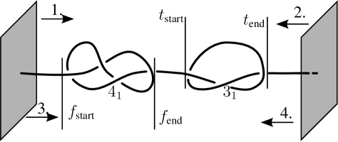
Figure 4: Schematic drawing of the knot size analysis. We start removing beads from the left hand side first ($1.$). When the Alexander polynomial yields neither composite nor $3_{1}$ knot the beginning of the $3_{1}$ knot is reached ($t_{\text{start}}$). Restarting this procedure from the right hand side ($2.$) gives us the end of the $3_{1}$ knot ($t_{\text{end}}$). For the $4_{1}$ knot we start from the left hand side again ($3.$) and change the criteria to neither composite nor $4_{1}$ knot which gives us $f_{\text{start}}$. Analogously $f_{\text{end}}$ is obtained.

For each configuration we confirm that there was no bond-crossing by computing $\Delta_{p}(-1.1)$. Now we start to reduce the chain from one side by successively removing beads starting with the first bead which is not fixed to the wall. The first remaining bead is connected to the fixed bead on the wall and the chain is thereby closed again. To determine the starting monomer of one knot, e.g., the $3_{1}$ knot $t_{\text{start}}$, we check after each reduction if the result of the Alexander polynomial is still the composite knot or the knot itself. The end of this knot is determined similarly by starting from the other end and applying the same criteria which leads to $t_{\text{end}}$. Likewise, we determine the start and the end monomer of the $4_{1}$ knot $f_{\text{start}}$ and $f_{\text{end}}$. A scheme of this process is shown in FIG. 4. With these four values we can calculate both knot centers $m_{1/2}$ on the x-axis by using the arithmetic mean.

III.4 Data analysis

The computational determination of knot sizes as described above typically results in strongly fluctuating data even if underlying structures are similar. This method immanent noise covers up relevant features of the transition such as the triple peak in FIG. 2b and the slightly increased size of the translocating knot in the intertwined state (FIG. 2d, compare with FIG. S1). It also (artificially) broadens the peaks of the probability distribution at the expense of the transition states. For this reason it is not recommended to apply the data analysis directly to raw data. Instead, we have chosen to smoothen the data by applying a running average over 100 adjacent data points. Note that the length of this interval has a minor influence on the barrier height as shown in FIG. S2.

IV Supporting Information

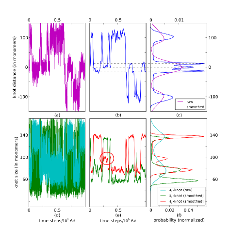
Figure S1: Same as FIG. 2, but including raw data in panel (a) and (d). If our analysis is applied directly to raw data, important features such as the occurrence of the triple peak in panel (c) and the slightly increased size of the translocating (figure-eight) knot in panel (f) are lost in the immanent noise of the detection method. The noise also results in an artificial broadening of the peaks in panel (c) and (f).

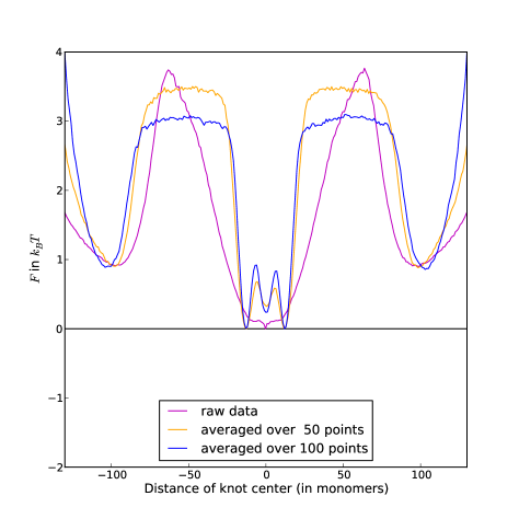
Figure S2: Free energy profiles for $\kappa=20k_{B}T$ and $D=88\sigma$ as derived from raw data (magenta) and derived after averaging over 50 (orange) and 100 (blue) data points (compare with FIG. 3b). In the raw data profile the noise artificially broadens the minima, which results in a sharper transition state. In addition, information on the triple peak is lost. Note that there is a small difference in the barrier height ($<0.5k_{B}T$) if we change the interval over which we average from $50$ to $100$ data points.

[h] http://www.pnas.org/content/111/22/7948.abstract This video shows a “knot tunneling” event. The starting configuration features a trefoil knot (colored in green) on the left hand side and a figure-eight knot (colored in red) on the right. The trefoil knot will diffuse through the enlarged figure-eight knot and swap positions with it at the end of the movie.

References

- (1) Thompson W. (1867) On vortex atoms. Philos. Mag. 34:15-24.
- (2) Mansfield M. L. (1994) Are there knots in proteins. Nature Structural Biology 1:213-214.
- (3) Taylor W. R. (2000) A deeply knotted protein structure and how it might fold. Nature 406:916-919.
- (4) Lua R. C., Grosberg A. Y. (2006) Statistics of knots, geometry of conformations, and evolution of proteins. Plos Computational Biology 2:350-357.
- (5) Virnau P., Mallam A., S. Jackson (2011) Structures and folding pathways of topologically knotted proteins. Journal of Physics-Condensed Matter 23:033101.
- (6) Potestio R., Micheletti C., Orland H. (2010) Knotted vs. unknotted proteins: Evidence of knot-promoting loops. Plos Computational Biology 6:e1000864.
- (7) Bölinger, D. et al. (2010) A stevedore’s protein knot PLoS computational biology 6:4
- (8) Nureki O. et al. (2004) Deep knot structure for construction of active site and cofactor binding site of trna modification enzyme. Structure 12:593-602.
- (9) King N. P., Jacobitz A. W., Sawaya M. R., Goldschmidt L., Yeates T. O. (2010) Structure and folding of a designed knotted protein. Proceedings of the National Academy of Sciences of the United States of America 107:20732-20737.
- (10) Liu L. F., Liu C. C., Alberts B. M. (1980) Type-ii dna topoisomerases - enzymes that can un-knot a topologically knotted dna molecule via a reversible double-strand break. Cell 19:697-707.
- (11) Dean F., Stasiak A., Koller T., Cozzarelli N. (1985) Duplex dna knots produced by escherichia-coli topoisomerase-i - structure and requirements for formation. Journal of Biological Chemistry 260:4975-4983.
- (12) Arsuaga J., Vazquez M., Trigueros S., Sumners D. W., Roca J. (2002) Knotting probability of dna molecules confined in restricted volumes: Dna knotting in phage capsids. Proceedings of the National Academy of Sciences of the United States of America 99:5373-5377.
- (13) Marenduzzo D., Micheletti C., Orlandini E. (2010) Biopolymer organization upon confinement. Journal of Physics-Condensed Matter 22:283102.
- (14) Arsuaga J. et al. (2005) Dna knots reveal a chiral organization of dna in phage capsids. Proceedings of the National Academy of Sciences of the United States of America 102:9165-9169.
- (15) Marenduzzo D., Micheletti C. (2003) Thermodynamics of dna packaging inside a viral capsid: The role of dna intrinsic thickness. Journal of Molecular Biology 330:485-492.
- (16) Reith D., Cifra P., Stasiak A., Virnau P. (2012) Effective stiffening of dna due to nematic ordering causes dna molecules packed in phage capsids to preferentially form torus knots. Nucleic Acids Research 40:5129-5137.
- (17) Bao X. R., Lee H. J., Quake S. R. (2003) Behavior of complex knots in single dna molecules. Physical Review Letters 91:265506.
- (18) Vologodskii A. (2006) Brownian dynamics simulation of knot diffusion along a stretched dna molecule. Biophysical Journal 90:1594-1597.
- (19) Millett K., Rawdon E., Stasiak A., Sulkowska J. (2013) Identifying knots in proteins. Biochemical Society Transactions 41:533-537.
- (20) Matthews R., Louis A. A., Yeomans J. M. (2009) Knot-controlled ejection of a polymer from a virus capsid. Physical Review Letters 102:88101.
- (21) Sulkowska J. I., Sulkowski P., Onuchic J. (2009) Dodging the crisis of folding proteins with knots. Proceedings of the National Academy of Sciences of the United States of America 106:3119-3124.
- (22) Branton D. et al. (2008) The potential and challenges of nanopore sequencing. Nature Biotechnology 26:1146-1153.
- (23) Rybenkov V. V., Cozzarelli N. R., Vologodskii A. V. (1993) Probability of dna knotting and the effective diameter of the dna double helix. Proceedings of the National Academy of Sciences of the United States of America 90:5307-5311.
- (24) Shaw S. Y., Wang J. C. (1993) Knotting of a dna chain during ring-closure. Science 260:533–536.
- (25) Rosa A., Di Ventra M., Micheletti C. (2012) Topological jamming of spontaneously knotted polyelectrolyte chains driven through a nanopore. Physical Review Letters 109:118301.
- (26) Halverson J. D., Lee W. B., Grest G. S., Grosberg A. Y., Kremer K. (2011) Molecular dynamics simulation study of nonconcatenated ring polymers in a melt. i. statics. Journal of Chemical Physics 134:204904.
- (27) Anderson J. A., Lorenz C. D., Travesset A. (2008) General purpose molecular dynamics simulations fully implemented on graphics processing units. Journal of Computational Physics 227:5342-5359.
- (28) Virnau P. (2010) Detection and visualization of physical knots in macromolecules. Physics Procedia 6:117-125.
- (29) Virnau P., Kantor Y., Kardar M. (2005) Knots in globule and coll phases of a model polyethylene. Journal of the American Chemical Society 127:15102-15106.
- (30) Vologodskii A. V., Anshelevich V. V., Lukashin A. V., Frank-Kamenetskii M. D. (1979) Statistical mechanics of supercoils and the torsional stiffness of the DNA double helix Nature 280:5720
- (31) Gross, P. et al. (2011) Quantifying how DNA stretches, melts and changes twist under tension Nature Physics 7:731–736
- (32) Saitta, M. A., Soper, P. D., Wasserman, E., Klein, M. L. (1999) Influence of a knot on the strength of a polymer strand Nature 399:6731 pp. 46–48
- (33) Saitta M. A., Klein M. L. (1999) Polyethylene under tensil load: Strain energy storage and breaking of linear and knotted alkanes probed by first-principles molecular dynamics calculations The Journal of chemical physics 111:20 pp. 9434–9440