Ergodicity and spectral cascades in point vortex flows on the sphere

Abstract

We present results for the equilibrium statistics and dynamic evolution of moderately large ($n={\mathcal{O}}(10^{2}-10^{3})$) numbers of interacting point vortices on the sphere under the constraint of zero mean angular momentum. For systems with equal numbers of positive and negative identical circulations, the density of re-scaled energies, $p(E)$, converges rapidly with $n$ to a function with a single maximum with maximum entropy. Ensemble-averaged wavenumber spectra of the nonsingular velocity field induced by the vortices exhibit the expected $k^{-1}$ behavior at small scales for all energies. Spectra at the largest scales vary continuously with the inverse temperature of the system. For positive temperatures, spectra peak at finite intermediate wavenumbers; for negative temperatures, spectra decrease everywhere. Comparisons of time and ensemble averages, over a large range of energies, strongly support ergodicity in the dynamics even for highly atypical initial vortex configurations. Crucially, rapid relaxation of spectra towards the microcanonical average implies that the direction of any spectral cascade process depends only on the relative difference between the initial spectrum and the ensemble mean spectrum at that energy; not on the energy, or temperature, of the system.

I Introduction

The point vortex model, originally developed by Kirchoff Kirchhoff (1876) as a limiting form of Euler’s equations in two-dimensions, continues to provide a conceptual and computational tool for understanding inviscid, nonlinear vortex dynamics in both traditional and superfluid turbulence (Suryanarayanan et al. (2014); Wang et al. (2007); Simula et al. (2014)). The multi-body Hamiltonian describing the dynamics of idealized point vortices serves as a paradigm for developing kinetic theories in systems dominated by long-range interactions Kiessling and Lebowitz (1997); Chavanis (2012).

The statistical mechanics of point vortex systems was first addressed in the seminal work of Onsager Onsager (1949) who observed that in a finite domain, the Hamiltonian structure of a system of sufficiently large numbers of positive and negative vortices implies the existence of ‘negative temperature’ equilibrium states which naturally exhibit clustering of like-signed vortices Eyink and Sreenivasan (2006). Onsager’s statistical approach has inspired a wealth of subsequent work on vortex-based, mean-field turbulence closures Montgomery and Joyce (1974); *LundPoint; *KraichnanMontgomery; *Miller; *Robert and the existence of negative temperature states has been interpreted (e.g. Bühler (2002); Yatsuyanagi (2005); Wang et al. (2007); Simula et al. (2014)) as an energy-conserving analog of self-organization via ‘vortex merger’ commonly observed in two-dimensional turbulence McWilliams (1983); Dritschel et al. (2008). To date, however, direct connections between Onsager’s equilibrium prediction for the inviscid point-vortex system and the up-scaling, inverse-energy cascade in two-dimensional Navier-Stokes turbulence have proved elusive.

Underpinning the equilibrium statistical mechanics approach are the assumptions that the system is both energy isolated (inviscid) and ergodic, namely that as $t\to\infty$, the system samples all possible configurations on a fixed energy surface. While the inviscid assumption is clearly violated by Navier-Stokes vortices, two-dimensional turbulence cascades energy to the largest scales where viscous effects are less pronounced. In addition, as long as the relaxation to equilibrium of the inviscid system takes place on time-scales much shorter than those imposed by viscosity, the equilibrium statistics of the inviscid model should approximate those of the full system on these timescales Eyink and Spohn (1993). Ergodicity of point-vortex systems remains an open issue. The assumption was questioned by Onsager Onsager (1949) and repeatedly since Weiss and McWilliams (1991); Tabeling (2002).

In the present work, we directly examine both ergodicity and the connection between equilibrium statistical properties and dynamic kinetic energy cascades for two-dimensional point-vortex systems on the unit sphere Zermelo (1902). The sphere has the distinct advantage of providing a bounded domain without the complications of imposing explicit boundary conditions via image particles (infinitely many for doubly-periodic domains). Despite its apparent attraction, there has been relatively little work addressing the statistical mechanics of point vortices on the sphere. Recently, for spherical systems with skewed distributions of vortex strengths, Kiessling & Wang (2012) Kiessling and Wang (2012) proved convergence to continuous solutions of Euler’s equations. The scaling limits considered, however, assume the existence of large-scale mean flows and thus have singular structure in the zero mean, zero angular momentum limit.

In closer analogy with turbulence studies, we study fluctuations in zero angular momentum states of binary populations of vortices with zero mean circulation (see, for example, Bühler (2002); Yatsuyanagi (2005); Weiss and McWilliams (1991)). We find that the kinetic energy spectrum of flows induced by such systems scales as $k^{-1}$, for sufficiently large degree (or wavenumber) $k$, independent of the system energy. As Onsager conjectured, increasing the energy of the system necessarily increases the kinetic energy content at the largest allowable scales. However, comparisons of microcanonical and time averaged two-point statistics show clear evidence of ergodicity in the vortex dynamics implying that the direction of any dynamic spectral evolution depends solely on the shape of the initial spectrum relative to the ensemble mean. Therefore, for the spherical system, there is no a priori association between negative temperature states and the inverse energy cascade.

II Equilibrium Statistics

Point vortices on a unit sphere evolve according to Hamilton’s equations, with conserved Hamiltonian

$$H=-\sum_{i=1}^{n}\sum_{j\neq i}\kappa_{i}\kappa_{j}\ln\left[\left(1-\mathbf{r}_{i}\cdot\mathbf{r}_{j}\right)/2\right].$$ (1)

Here $\kappa_{i}$ is the ‘strength’ (circulation$/4\pi$) of vortex $i$ and $\mathbf{r}_{i}$ its position ($|\mathbf{r}_{i}|=1$). The evolution equations are

$$\frac{d\mathbf{r}_{i}}{dt}=2\sum_{j\neq i}\kappa_{j}\frac{\mathbf{r}_{i}\times\mathbf{r}_{j}}{1-\mathbf{r}_{i}\cdot\mathbf{r}_{j}}.$$ (2)

In addition to $H$, the vector angular impulse, ${\mathbf{I}}=\sum_{i=1}^{n}\kappa_{i}\mathbf{r}_{i}$, is also conserved although only the angular momentum, $|{\mathbf{I}}|$, affects the statistical properties.

We consider systems with $\kappa_{i}=\pm 1$, and zero net circulation. The pairwise interaction energies are

$$q_{ij}=\pm\ln\left[\left(1-\mathbf{r}_{i}\cdot\mathbf{r}_{j}\right)/2\right].$$ (3)

For randomly placed vortices, the argument of the logarithm is uniformly-distributed over $(0,1)$. Thus, $q_{ij}$ is exponentially-distributed over $(0,\infty)$ where $\langle q_{ij}\rangle=1$ and over $(-\infty,0)$ where $\langle q_{ij}\rangle=-1$. In particular,

$$\langle H\rangle=\sum_{i=1}^{n}\sum_{j\neq i}\langle q_{ij}\rangle=2\left(\frac{n}{2}(\frac{n}{2}-1)-(\frac{n}{2})^{2}\right)=-n.$$

For any distribution of vortex strengths with identical numbers of opposite-signed circulations, similar cancellations occur and $\langle H\rangle=O(n)$ Bühler (2002); Yatsuyanagi (2005); Esler et al. (2013) rather than $\langle H\rangle=O(n^{2})$ Kiessling and Wang (2012). Given exponential $q$ statistics, the standard deviation of $H$ is also $O(n)$. In this case, the joint density of states, $W_{H}(\tilde{E},\tilde{J})=$

$$\int_{S^{2n}}\delta(\tilde{E}-H(\mathbf{r}_{1},\ldots,\mathbf{r}_{n}))\,\delta(\tilde{J}-|\mathbf{I}(\mathbf{r}_{1},\ldots,\mathbf{r}_{n})|)d\mathbf{r}_{1}\ldots d\mathbf{r}_{n}$$

has a limiting function $p(E,J)=\lim_{n\to\infty}nW_{H/n}(\tilde{E},\tilde{J})$ for the specific energy $E=\tilde{E}/n$ and re-scaled angular momentum $J=\tilde{J}/\sqrt{n}$.

The re-scaled density has been computed numerically by sampling $10^{9}$ uniformly-distributed placements of $n=200$ vortices. In this case, $\langle E\rangle=-1.0000$, as expected, with $\langle J\rangle=0.9215$. The observed distribution is asymmetric with a single maximum at $\left(E,J\right)=\left(-1.684,0.824\right)$, significantly different from the mean.

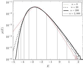
Figure 1: (a) Distribution function $p(E)$ computed from $10^{7}$ samples for different numbers of vortices $n$. Vertical lines correspond to the 9 energy levels for $n=200$ considered in the text. (b) Corresponding inverse temperatures $\beta(E)$.

Direct extraction of $p(E):=p(E,J=0)$ from the joint density is computationally expensive; estimates can be obtained more efficiently by adjusting random states towards $J=0$. From a single realization of $n$ randomly-generated vortex positions, we compute ${\mathbf{I}}$ and then displace each vortex by $-\kappa_{i}{\mathbf{I}}/n$. This sets $J=0$, but the vortices no longer reside on the spherical surface. Re-scaling each $\mathbf{r}_{i}$ by $|\mathbf{r}_{i}|$ produces a new ${\mathbf{I}}$, and the process is iterated until convergence. For $n=200$, $p(E)$ computed this way was found to be identical within sampling errors to $p(E,J<0.2)$ estimated from the joint density.

For fixed $n$, $p(E)$ was estimated by binning $10^{7}$ samples of $n$ uniformly distributed vortex positions iterated to $J<10^{-14}$. The resulting density and inverse temperature, $\beta=d\ln{p(E)}/dE$, are shown for varying $n$ in Fig. 1. While nearly symmetric for small $n$, the scaled density converges rapidly to a skewed distribution as $n$ increases. The scaled inverse temperature asymptotes to a fixed, negative value at large positive energies Pointin and Lundgren (1976); Yatsuyanagi (2005); Esler et al. (2013). There is little difference in either the density of states or the temperature when $n$ increases beyond 200.

III Kinetic Energy Spectra

Much has been intimated about Onsager’s statistical theory of self-organization and the widely-observed scale cascade of kinetic energy in direct simulations of two-dimensional turbulence Eyink and Sreenivasan (2006); Bühler (2002); Yatsuyanagi (2005). The scale cascade results in the accumulation of energy at the domain scale, i.e. a global-scale flow Qi and Marston (2014).

To compare the dynamic evolution of point vortices to microcanonical ensemble predictions, we consider two statistical measures of the vortex population. Both quantify any scale cascade or statistical change in the vortex population, though neither have been examined before in this context. First, as in nearly all studies of two-dimensional turbulence, we examine the kinetic energy spectrum $K(k)$ where $k$ is the wavenumber magnitude (spherical harmonic degree). $K(k)$ is calculated by evaluating the streamfunction

$$\psi(\mathbf{r})=\sum_{i=1}^{n}\kappa_{i}\ln\left[\left(1-\mathbf{r}_{i}\cdot\mathbf{r}\right)/2\right]$$ (4)

induced by the vortices at every point $\mathbf{r}$ on a regular latitude-longitude grid (1024 $\times$ 2048 points). The Fourier-Legendre transform of $\psi$ and its (power) spectrum $P(k)$ are then computed and we obtain $K(k)$ from $k(k+1)P(k)$. While the total kinetic energy is singular as a result of the $k^{-1}$ spectral tail, the spectrum $K(k)$ is well behaved for finite $k$.

A complementary Lagrangian measure of the vortex population is given by the probability distribution $p_{\rm int}(q)$ of the pair-wise energy  (3). To explicitly highlight anomalous distributions of dipoles or like-signed clusters, we consider the residual probability $p^{\prime}_{\rm int}\equiv p_{\rm int}-e^{-|q|}/2$ by subtracting the exponential distribution produced by uniform, random placement.

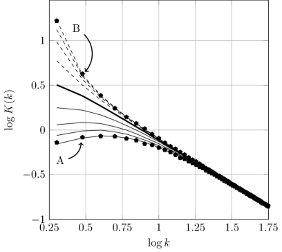
Figure 2: Microcanonical kinetic energy spectra, $K(k)$ for the nine energies considered. $K$ at low wavenumbers increases monotonically with energy $E$ from A to B. $\beta>0$ states shown in solid, $\beta<0$ states dashed and $\beta\sim 0$ in bold. Solid circles indicate time averages of dynamical evolution.

For $n=200$, these two statistics are computed by sampling $10^{4}$ states within each of nine energy ranges centered around the vertical lines shown in Fig. 1a. The energy ranges include both positive and negative temperature states, and are narrow – the probability of finding a state in a given range never exceeds $3.7\times 10^{-5}$.

All nine individual kinetic energy spectra shown in the upper panel of Fig. 2 converge to the expected $k^{-1}$ form at small scales. Consistent with Onsager’s predictions, positive temperature (strongly negative $E$) states have the least kinetic energy at largest scales. The kinetic energy content at the largest scales increases continuously as $E$ increases and the system transitions to negative temperature states. Notably, the spectral slope at small $k$ changes from values above $-1$ to below $-1$ near $\beta=0$.

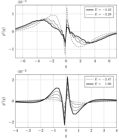
Figure 3: The residual probability $p^{\prime}_{\rm int}$ versus normalized vortex interaction energy, $q$ for (a) lower range of energies considered and (b) higher range of energies (note change of scales).

The low energy ($\beta>0$) spectra are consistent with dipole spectra produced by randomly placing pairs of opposite-signed vortices. Such spectra are depleted at low $k$ and, as $E$ decreases, approach $k^{1}$ at the large scales. The surplus of dipoles for positive $\beta$ states is seen in $p^{\prime}_{\rm int}(q)$ shown in Fig. 3. Like the kinetic energy spectrum, $p^{\prime}_{\rm int}$ exhibits a monotonic dependence on $E$ with a surplus of closely-spaced dipoles having $q\ll-1$ at low $E$, while at high $E$ ($\beta<0$) there is a surplus of closely-spaced like-signed pairs (binaries) having $q\gg 1$ together with a deficit of closely-spaced dipoles. Importantly, both complementary statistics, $\langle K\rangle(k)$ and $\langle p^{\prime}_{\rm int}\rangle(q)$, vary continuously with the inverse system temperature $\beta$. There is no abrupt change in either at the transition from positive to negative temperatures.

IV Ergodicity and Spectral Cascade

We now turn our attention to the question of ergodicity by quantifying the connection between time-averaged statistics of dynamically evolved states and microcanonical ensemble measures. The evolution equation (2) is solved in parallel using a 4th order Runge-Kutta scheme with an adaptive time step to ensure exact conservation of momentum and energy preservation to $10^{-7}$. As such, numerical variations in the dynamically evolved energy are always smaller than the width of the energy bins used to construct microcanonical statistics. With $n=200$, a single state in each of the 9 energy ranges was evolved for $400$ time units. Redefining the vortex strengths as $\kappa_{i}=\pm 1/\sqrt{n}$, gives $E=H$ directly from (1) and a characteristic timescale is then $\tau=\pi\bar{d}^{2}/|\kappa_{i}|=4\pi^{2}/\sqrt{n}$, approximately $2.79$ for $n=200$.

The kinetic energy spectra and $\langle p^{\prime}_{\rm int}\rangle(q)$, time-averaged over the entire evolution were found to be almost identical to the microcanonical ensemble results. The resulting time averaged kinetic energy spectra, $\overline{K}(k)$, for the two extreme energies $E=-4.42$ and $1.66$ indicated by solid circles in Fig. 2 are virtually indistinguishable from the microcanonical estimates. The same is found for $\langle p^{\prime}_{\rm int}\rangle(q)$. In contrast to previous results for $n=6$ vortices in a doubly-periodic domain Weiss and McWilliams (1991), here for $n=200$ vortices on the sphere there is strong evidence of ergodicity, independent of the energy or temperature of the system.

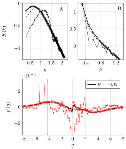
Figure 4: Top panels: Evolution of the kinetic energy spectra, $K(k)$ for (A) low-energy, positive temperature ($E=-4.42$) and (B) high-energy, negative temperature ($E=1.66$). The initial spectra are shown by $+$, the long time spectra by $\circ$ and the microcanonical estimate (from Fig. 2) is bold. Dashed lines indicate results for short times. Bottom panel: Evolution of residual probability $p^{\prime}_{int}$ for case A. Symbols are the same as above.

As a yet stronger test of ergodicity, we consider the evolution of states with atypical initial spectra for a given energy. First, an ensemble of 111 states was generated in the strongly positive temperature ($E\sim-4.42$) system by randomly placing vortex dipoles (opposite signed pairs separated by $\bar{d}/\sqrt{2}$) instead of single vortices. For such dipole states, the kinetic energy spectrum $\langle K\rangle(k)$ (averaged over the 111 states), shown by the $+$ symbols in Fig. 4A, differs significantly (beyond several microcanonical standard deviations) from the microcanonical mean (thick solid line). However, upon evolution the dipole initial states rapidly relax towards the microcanonical mean. The dipole spectrum time averaged over $2\leq t\leq 4$ is shown by the dashed line, and the late time-averaged spectrum ($392\leq t\leq 400$, open circles) is statistically indistinguishable from the microcanonical estimate. In addition, the standard deviation in the spectrum also converges to that of the microcanonical ensemble (not shown).

Vortex interactions immediately destroy the initial equal vortex-pair separation, and the distribution of pair separations continues to spread until the state resembles a randomly chosen collection of vortices for this energy. As shown in the lower panel of Fig. 4, the initial residual probability $p^{\prime}_{\rm int}(q)$ spikes at the $q$ value of the dipole separation, but then relaxes to the microcanonical estimate (open circles show the late time average). This relaxation can be seen directly in the streamfunction of any dipole initial condition. The left panels of fig. 5 shows the evolution of $\psi(\theta,\phi)$ from an initial dipole state (a1) to $t=400$ (a2) along with the streamfunction of a randomly chosen member of the microcanonical ensemble (a3). For this positive temperature state, there is an inverse cascade of kinetic energy to large scales.

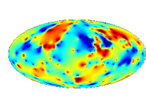
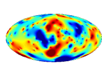
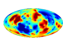
Figure 5: (Color online) Left panels: Evolution of the dipole streamfunction at $E=-4.42$. (a1) Initial dipole streamfunction. (a2) dipole streamfunction at $t=400$. (a3) Initial streamfunction for a representative ensemble member at the same energy. Right panels: Same as left but for forward cascade case, $E=1.66$. The projection shows the entire sphere and the color scale is constant for each energy.

Similar results have been found starting from atypical states in the highest energy range, $E\sim 1.66$ where the temperature is negative. By randomly placing vortices with an increased probability to project on the $k=2$ spherical harmonic, a surplus of kinetic energy is created at the largest permissible scale for $J=0$. As seen in Fig. 4B, the initial $\langle K\rangle(k)$ ($+$ symbols) again rapidly relaxes back to the microcanonical estimate (bold line) with the dashed line showing the spectrum at times $2\leq t\leq 4$ and the open circles the late time spectrum. Corresponding behavior in real space for an individual initial condition is shown in the right column of Fig. 5, with an initial atypical state in (b1) (the pattern closely matches a spherical harmonic), the same state at $t=400$ (b2), and a randomly selected member of the microcanonical ensemble (b3). The images in (b2) and (b3) exhibit more smaller-scale features than the image in (b1) and, as shown in the spectral evolution, there is a forward cascade of kinetic energy despite the negative system temperature.

The relaxation of atypical states to the microcanonical average occurs on a short timescale, comparable to the rotation period $\tau$ of two like-signed vortices separated by a distance $\bar{d}$ (also the time taken for a dipole pair to propagate a distance $\bar{d}$). That is, any special order in the initial conditions is rapidly destroyed by the ensuing dynamical evolution. This is a strong indication of ergodic dynamics in this geometry, and appears to contrast with the results of Weiss and McWilliams (1991) in doubly-periodic geometry. On the other hand, Weiss and McWilliams (1991) considered just 6 vortices. It might be that so few vortices have insufficient freedom to fully randomize and resemble typical, microcanonical states.

To test this, we repeated the analysis above for $n=8$ vortices in spherical geometry. After accounting for additional constraints arising from conservation of angular impulse ${\mathbf{I}}$, the two systems have a similar number of degrees of freedom. Here, we focus on the evolution of atypical low energy states, with $E\approx-4.42$. These states were generated by placing 4 pairs of dipoles at random, with the halves of each pair separated by $d=2e^{E/2}\approx 0.22$. At this distance, the individual energies of the dipoles sum to $E$. The additional energy contributed by inter-pair interactions is ${\mathcal{O}}(d^{2}/\bar{d}^{2})\ll 1$ and is easily canceled by appropriate placement of the pairs.

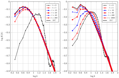
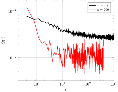
Figure 6: Evolution of the kinetic energy spectrum for dipole initial conditions at $E=-4.42$ for $n=200$ (upper left panel) and $n=8$ (upper right panel). Lower panel shows the temporal evolution of the $Q$ measure for the two cases.

The upper panels of Fig. 6 contrast the ensemble-averaged spectral evolution of atypical states for $n=200$ (seen before) on the left with that for $n=8$ on the right. For $n=8$, the ensemble consists of 1000 states (an increase on the 111 states used for $n=200$ to reduce the variance in $K(k)$). Both systems clearly show spectral relaxation to the microcanonical mean. The relaxation rate, however, is much slower in the dilute, $n=8$ case.

Another measure of relaxation is obtained by analyzing the probability distribution $p_{\rm int}(q)$ of the normalized pairwise interaction energies in (3). Denote $\bar{p}_{\rm int}(q)$ as the microcanonical ensemble mean, and $\bar{\delta}_{\rm int}$ as the integrated standard deviation of individual members of the ensemble from $\bar{p}_{\rm int}(q)$. We measure the relaxation of the dynamical ensemble to the microcanonical one by $Q(t)\equiv{\delta}_{\rm int}(t)/\bar{\delta}_{\rm int}$ where ${\delta}_{\rm int}$ is the integrated standard deviation of individual members of the dynamical ensemble from $\bar{p}_{\rm int}(q)$. This measure is shown in the bottom panel of Fig. 6 (note logarithmic scales). Consistent with the spectral evolution, $Q(t)$ for $n=200$ decreases rapidly to a low, fluctuating level (the logarithmic scaling makes this fluctuation appear much larger than it actually is). By contrast, the decay of $Q(t)$ is much slower for $n=8$, though nonetheless it approaches a roughly constant level at late times. The higher equilibrated level for $n=8$ is predominantly due to differences in the statistical sample size. The calculation of $p_{\rm int}(q)$ involves $n(n-1)/2$ separate vortex interactions. This is substantially larger for $n=200$ than for $n=8$, and while 9 times more cases were considered for $n=8$, the sample size is still approximately 80 times larger for $n=200$ than for $n=8$.

The results show that atypical dynamical states inevitably relax to the equilibrium microcanonical distribution, independent of the system size (at least for $n\geq 8$). Equilibration is observed in both the kinetic energy spectra $K(k)$ and in the complementary measure $Q$ using $p_{\rm int}(q)$.

Although relaxation is observed both for $n=8$ and $n=200$, there is a striking difference in the rate of relaxation in the two cases. For $n=200$, we have found that the relaxation occurs on the characteristic timescale $\tau$, whereas for $n=8$ it is considerably slower. Given that the circulations are scaled by $\sqrt{n}$, the characteristic timescale is independent of system size. Therefore, the observed difference in relaxation timescales cannot be explained simply by differences between dipole collision rates in the two systems.

Movies of the vortex motion in the dilute dipole case indicate that a majority of dipole interactions involve only simple particle exchange, producing no discernible change in the separation of the vortices in each pair. Such interactions preserve the structure of the initial conditions and rapid statistical evolution requires higher-order collisions involving interactions between three or more dipole pairs. Evidence that such interactions occur far less frequently in the $n=8$ case is provided in Fig. 7. Here we show the early time evolution of the pairwise energy, $q_{ij}$, of 4 initial dipoles — the complete set when $n=8$, and 4 randomly selected from the 100 available when $n=200$. Particle exchange collisions are clearly evident in the dilute case ($n=8$, upper panel) where individual pair energies spike to zero before consistently returning to the negative energy level associated with their initial separations. Two dipoles pairs repeat this process more than 5 times in the first 10 time units. The time distribution of pairwise energies is bimodal, highly concentrated at $-|q_{0}|$ and 0. By contrast, initial pairs in the $n=200$ case are rapidly scattered and information about the interaction energy of the initial configuration is quickly lost. This is true not only for the 4 selected dipole pairs shown here, but for all pairs in the $n=200$ case.

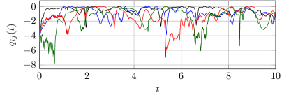
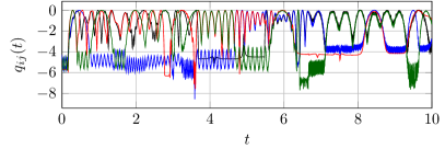
Figure 7: Evolution of the pairwise energy for (top panel) the 4 initial dipoles for $n=8$ and (lower panel) 4 initial dipoles in the $n=200$ case.

V Conclusions

Due to the universal $k^{-1}$ behavior of point-vortex kinetic energy spectra at small scales, increasing the system energy preferentially increases the kinetic energy content at the largest allowable scales. While this is entirely consistent with Onsager’s conjecture concerning the increased likelihood of observing large-scale structure at sufficiently high energies, notably it is also independent of the thermodynamic temperature of the system. In addition, the results indicate that point-vortex dynamics, at least on the isotropic sphere, are ergodic and therefore statistical measures derived from the dynamics of almost all initial states simply relax to those given by the microcanonical ensemble. For the kinetic energy spectra (equivalently $p_{int}(q)$ distributions) examined here, the relaxation takes place on timescales comparable to an eddy turnover time, independent of the system temperature. As such, for the simplest bounded domain, there is no direct relationship between the sign of the statistical temperature and the direction of any dynamic cascade process in the velocity field induced by a finite number of point vortices.

ACP supported under DOD (MURI) grant N000141110087 ONR. The computations were supported by the CUNY HPCC under NSF Grants CNS-0855217 and CNS-0958379. The authors thank C. Lancellotti for fruitful discussions.

References

- Kirchhoff (1876) G. Kirchhoff, Vorlesungen über mathematische Physik (Teubner, Leipzig, 1876).
- Suryanarayanan et al. (2014) S. Suryanarayanan, R. Narasimha, and N. D. H. Dass, Phys. Rev. E 89, 013009 (2014).
- Wang et al. (2007) S. Wang, Y. Sergeev, C. Barenghi, and M. Harrison, J. Low Temp. Phys. 149, 65 (2007).
- Simula et al. (2014) T. Simula, M. J. Davis, and K. Helmerson, Phys. Rev. Lett. 113, 165302 (2014).
- Kiessling and Lebowitz (1997) M.-H. Kiessling and J. Lebowitz, Lett. Math. Phys. 42, 43 (1997).
- Chavanis (2012) P.-H. Chavanis, Phys. A 391, 3657 (2012).
- Onsager (1949) L. Onsager, Nuovo Cimento 6, 279 (1949).
- Eyink and Sreenivasan (2006) G. Eyink and K. Sreenivasan, Rev. Modern Phys. 70, 87 (2006).
- Montgomery and Joyce (1974) D. Montgomery and G. Joyce, Phys. Fluids 17, 1139 (1974).
- Lundgren and Pointin (1977) T. Lundgren and Y. Pointin, J. Stat. Phys. 17, 323 (1977).
- Kraichnan and Montgomery (1980) R. Kraichnan and D. Montgomery, Rep. Prog. Phys 43, 547 (1980).
- Miller (1990) J. Miller, Phys. Rev. Lett. 65, 2137 (1990).
- Robert and Sommeria (1992) R. Robert and J. Sommeria, Phys. Rev. Lett. 69, 2776 (1992).
- Bühler (2002) O. Bühler, Phys. Fluids 14, 2139 (2002).
- Yatsuyanagi (2005) Y. Yatsuyanagi, Phys. Rev. Lett. 94, 0544502 (2005).
- McWilliams (1983) J. McWilliams, J. Fluid Mech. 146, 21 (1983).
- Dritschel et al. (2008) D. Dritschel, R. Scott, R.K., C. MacAskill, G. Gottwald, and C.V.Tran, Phys. Rev. Lett. 101, 094501 (2008).
- Eyink and Spohn (1993) G. Eyink and H. Spohn, J. Stat. Phys. 70, 833 (1993).
- Weiss and McWilliams (1991) J. Weiss and J. McWilliams, Phys. Fluids A 3, 835 (1991).
- Tabeling (2002) P. Tabeling, Phys. Rep. 362, 1 (2002).
- Zermelo (1902) E. Zermelo, Z. Math. Phys. 47, 201 (1902).
- Kiessling and Wang (2012) M. Kiessling and Y. Wang, J. Stat. Phys. 148, 896 (2012).
- Esler et al. (2013) J. Esler, T. Ashbee, and N. McDonald, Phys. Rev. E 88, 012109 (2013).
- Pointin and Lundgren (1976) Y. Pointin and T. Lundgren, Phys. Fluids 19, 1459 (1976).
- Qi and Marston (2014) W. Qi and J. B. Marston, J. Stat. Mech. 2014, 07020 (2014).