The space density of magnetic and non-magnetic cataclysmic variables, and implications for CV evolution

Abstract

We present constraints on the space densities of both non-magnetic and magnetic cataclysmic variables, and discuss some implications for models of the evolution of CVs. The high predicted non-magnetic CV space density is only consistent with observations if the majority of these systems are extremely faint in X-rays. The data are consistent with the very simple model where long-period IPs evolve into polars and account for the whole short-period polar population. The fraction of WDs that are strongly magnetic is not significantly higher for CV primaries than for isolated WDs. Finally, the space density of IPs is sufficiently high to explain the bright, hard X-ray Galactic Centre source population.

Keywords: Cataclysmic variables - Dwarf novae - Nova-likes - Intermediate polars - Polars - X-rays.

 

1 Introduction

There are still many uncertainties in the theory of cataclysmic variable (CV) formation and evolution, as well as several serious discrepancies between predictions and the properties of the observed CV population (e.g. Patterson 1998; Pretorius, Knigge & Kolb 2007a; Pretorius & Knigge 2008a,b; Knigge, Baraffe & Patterson 2011). In order to constrain evolution models, more and better observational constraints on the properties of the Galactic CV populations are needed. A fundamental parameter predicted by evolution theory, that is expected to be more easily measured than most properties of the intrinsic CV population, is the space density, $\rho$. A few specific, important open questions concerning the formation and evolution of CVs:

• Is the large predicted population of non-magnetic CVs at short orbital period consistent with the current observed CV sample?

• Is there an evolutionary relationship between IPs and polars?

• Can the intrinsic fraction of mCVs be reconciled with the incidence of magnetic WDs in the isolated WD population?

• Do mCVs dominate the total Galactic X-ray source populations above $L_{X}\sim 10^{31}\,{\rm ergs^{-1}}$?

These questions can be addressed empirically, with reliable measurements of the space densities of the different populations of CVs.

Uncertainty in $\rho$ measurements is in part caused by statistical errors, arising from uncertain distances and small number statistics. However, the dominant source of uncertainty is most likely systematic errors caused by selection effects. Fig. 1 shows some reported measurements (differing by several orders of magnitude for non-magnetic CVs).

Selection effects are most easily accounted for in samples with simple, well-defined selection criteria. In the absence of a useful volume-limited CV sample, a purely flux-limited sample is the most suitable for measuring $\rho$. Whereas optical CV samples always include selection criteria based on, e.g., colour or variability, there are X-ray selected CV samples that are purely flux-limited. All active CVs show X-ray emission generated in the accretion flow. Furthermore, mCVs are luminous X-ray sources, while the correlation between the ratio of optical to X-ray flux and the optical luminosity of non-magnetic CVs, implies that an X-ray flux limit does not introduce as strong a bias against short-period CVs as an optical flux limit (e.g. van Teeseling et al. 1996).

Here we use 2 X-ray surveys, the ROSAT Bright Survey (RBS; e.g. Schwope et al. 2002), and the ROSAT North Ecliptic Pole (NEP) survey (e.g. Henry et al. 2006) to construct X-ray flux-limited CV samples. We then provide robust observational constraints on the space densities of both magnetic and non-magnetic CVs, by carefully considering the uncertainties involved.

We provide additional background on the questions listed above in Section 2, present the measurements in Section 3, discuss the implications of the results in Section 4, and finally list the conclusions in Section 5.

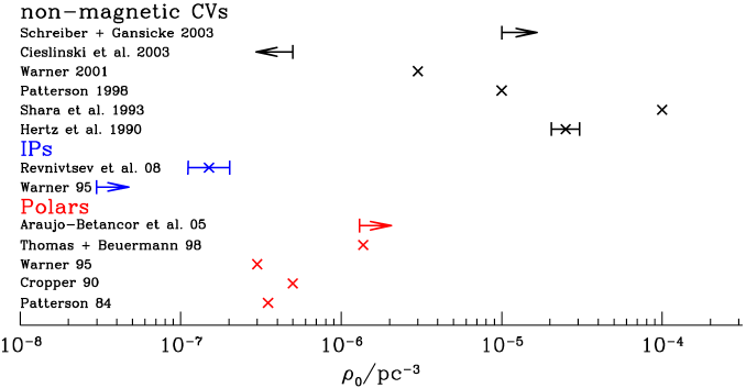
Figure 1: Some previously reported measurements of the space densities of different CV populations.

2 Context

2.1 Missing non-magnetic CVs

It is not clear whether the present-day observed non-magnetic CV population is inconsistent with theoretical expectations. Population synthesis models predict that only $\simeq 1$ percent of all CVs are above the period gap (see e.g. Kolb 1993). The the vast majority of CVs should therefore be intrinsically faint. Pretorius et al. (2007a) and Pretorius & Knigge (2008b) used a specific model of Kolb (1993), together with models of the outburst properties and SEDs of CVs, to show that, although observed CV samples are strongly biased against short-period systems, an as yet undetected faint CV population cannot dominate the overall population to the extent predicted by this particular population synthesis model. Knigge et al. (2011) used the properties of CV donor stars to conclude that the AML rate is lower above the gap and higher below the gap than predicted by the standard model. This leads to larger predicted factions of both period bouncers and long-period systems. Whether this is consistent with observed CV samples is not yet known.

That a large faint population of CVs exists is now clear from observations (Gansicke et al. 2009; Patterson 2011). However, whether observations have truly revealed a population as large as predicted remains to be seen.

Some predicted values of the non-magnetic CV space density are as high as $2\times 10^{-4}\,\mathrm{pc^{-3}}$ (de Kool 1992; Kolb 1993); observational estimates are typically much lower, but have a large range; values from $\leq 5\times 10^{-7}\mathrm{pc}^{-3}$ to $\rho\sim 10^{-4}\mathrm{pc}^{-3}$ have been reported. Perhaps the most straight forward test of these predictions is to compare them to the measured space density of the Galactic short-period, non-magnetic CV population.

2.2 Evolutionary relationship between IPs and polars

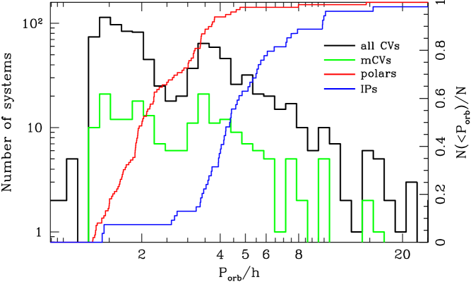
Figure 2: The orbital period distribution of all CVs (black), and mCVs (green). Cumulative distributions are also shown for polars (red) and IPs (blue). Almost all IPs are found at long $P_{orb}$, while most polars are short-$P_{orb}$ systems. Periods from Ritter & Kolb (2003).

In many ways, the formation and evolution of magnetic and non-magnetic CVs is thought to be similar. Both types of systems form through common envelope (CE) evolution, evolve first from long to short $P_{orb}$ because of angular momentum loss (AML), and eventually experience period bounce, when the thermal time-scale of the donor becomes longer than its mass loss time-scale. In fact, the main proposed difference between the evolution of mCVs and non-magnetic CVs affects only the polars, where magnetic braking (MB) is likely to be suppressed (e.g. Li & Wickramasinghe 1998; Townsley & Gansicke 2009). The $P_{orb}$ distributions of magnetic and non-magnetic CVs are broadly in line with these ideas: if polars and IPs are considered jointly, their $P_{orb}$ distribution is very similar to that of non-magnetic CVs, showing a period gap in the range $2\,{\rm hr}\raisebox{-2.58334pt}{$\,\stackrel{{\scriptstyle\raisebox{-0.60275pt}{$\textstyle<$}}}{{\sim}}\,$}P_{orb}\raisebox{-2.58334pt}{$\,\stackrel{{\scriptstyle\raisebox{-0.60275pt}{$\textstyle<$}}}{{\sim}}\,$}3\,{\rm hr}$ and a period minimum at around $P_{orb}\simeq 80\,{\rm min}$ (see Fig. 2).

It has been known for a long time that most IPs are found above the period gap and most polars below (Fig. 2)., which immediately suggests that IPs may evolve into polars (e.g. Chanmugam & Ray 1984). This is a physically appealing idea, since smaller orbital separation and lower $\dot{M}$ (besides large magnetic field strength) favour synchronization. MB drives much higher mass-transfer rates above the period gap than gravitational radiation (GR) does below; therefore, it is plausible that many accreting magnetic WDs may only achieve synchronization once they have crossed the period gap.

The main problem with this scenario is that the magnetic fields of the WDs in IPs ($B_{IP}\raisebox{-2.58334pt}{$\,\stackrel{{\scriptstyle\raisebox{-0.60275pt}{$\textstyle<$}}}{{\sim}}\,$}10{\rm MG}$) are systematically weaker than those of the WDs in polars ($B_{polar}\sim 10-100{\rm MG}$). There are several possible resolutions to this problem. Perhaps the simplest (in terms of binary evolution) is that the high accretion rates in IPs could partially “bury” the WD magnetic fields, so that the observationally inferred field strengths for these systems are systematically biased low (Cumming 2002). It is also possible that the short-period polar population is dominated by systems born below the period gap (this still requires an explanation for the fate of long-period IPs, although they may simply become unobservable; see Patterson 1994; Wickramasinghe, Wu & Ferrario 1991).

One way to shed light on the relationship between IPs and polars is via their respective space densities. For example, if all long-period IPs evolve into short-period polars, and all short-period polars are the progeny of long-period IPs, then their space densities should be proportional to the evolutionary time-scale associated with these phases. In this particular example, we would predict that $\rho_{polar}/\rho_{IP}\simeq\tau_{GR}/\tau_{MB}>>1$.

2.3 Intrinsic fraction of mCVs

Magnetic systems make up $\simeq 20\%$ of the known CV population (Ritter & Kolb 2003). At first sight, this is a surprisingly high fraction, given that the strong magnetic fields characteristic of IPs and polars ($B\raisebox{-2.58334pt}{$\,\stackrel{{\scriptstyle\raisebox{-0.60275pt}{$\textstyle>$}}}{{\sim}}\,$}10^{6}\,{\rm G}$) are found in only $\simeq 10\%$ of isolated WDs (e.g. Kulebi et al. 2009). If these numbers are representative of the intrinsic incidence of magnetism amongst CVs and single WDs, the difference between them would have significant implications: either strong magnetic fields would have to favour the production of CVs, or some aspect(s) of pre-CV evolution would have to favour the production of strong magnetic fields (see e.g. Tout et al. 2008).

However, it is actually by no means clear yet that magnetism is really more common in CV primaries than in isolated WDs. The main problem is that the observed fraction of magnetic systems amongst known CVs is almost certainly affected by serious selection biases. For example, since mCVs are known to be relatively X-ray bright, they are likely to be over-represented in X-ray-selected samples. Conversely, polars, in particular, are relatively faint in optical light (since they do not contain optically bright accretion disks), so they are likely to be under-represented in optically-selected samples. Given that the overall CV sample is a highly heterogeneous mixture of X-ray-, optical- and variability-selected sub-samples (which also usually lack clear flux limits), it is very difficult to know how the observed fraction of mCVs relates to the intrinsic fraction of magnetic WDs in CVs.

2.4 Galactic X-ray Source Populations

There have been many attempts to determine the make-up and luminosity function of Galactic X-ray source populations in a variety of environments, including the Milky Way as a whole, the Galactic Centre, the Galactic Ridge, and globular clusters. Remarkably, in all of these environments, mCVs have been proposed as the dominant population of X-ray sources above $L_{X}\raisebox{-2.58334pt}{$\,\stackrel{{\scriptstyle\raisebox{-0.60275pt}{$\textstyle>$}}}{{\sim}}\,$}10^{31}{\rm ergs^{-1}}$.

In most of these studies, the breakdown of the observed X-ray source samples into distinct populations is subject to considerable uncertainty, since few of the sources have optical counterparts and/or properties that permit a clear classification. Identifications of observed sources with physical populations rely mainly on X-ray luminosities and hardness, and statistical comparisons of observed and expected number counts. The local space densities of the relevant populations are arguably the most important ingredient in these comparisons. In effect, the question being asked is whether the extrapolation of the local space density to the environment being investigated can account for the observed number of sources seen there. In the case of mCVs, such extrapolations are difficult, primarily because the local space densities are rather poorly constrained.

3 Calculating space densities

3.1 The flux-limited samples

The RBS covers $|b|>30^{\circ}$ to $F_{X}\raisebox{-2.58334pt}{$\,\stackrel{{\scriptstyle\raisebox{-0.60275pt}{$\textstyle>$}}}{{\sim}}\,$}10^{-12}\mathrm{erg\,cm^{-2}s^{-1}}$, and includes 16 non-magnetic CVs, and 30 mCVs (6 IPs and 24 polars). The NEP covers 81 sq.deg. to $F_{X}\raisebox{-2.58334pt}{$\,\stackrel{{\scriptstyle\raisebox{-0.60275pt}{$\textstyle>$}}}{{\sim}}\,$}10^{-14}$. Only 4 CVs where detected in the NEP, all of them non-magnetic. The samples are presented in Pretorius et al. (2007b), Pretorius & Knigge (2012), and Pretorius et al. (2013).

3.2 The method

We use the $1/V_{max}$ method (e.g. Stobie et al. 1989) together with a Monte Carlo simulation designed to sample the full parameter space allowed by the data, as described in Pretorius et al. (2007b) and Pretorius & Knigge (2012). We tested the method to verify that it gives reliable error estimates, and also considered various possible systematic biases (Pretorius & Knigge 2012; Pretorius et al. 2013).

3.3 Results

3.3.1 Probability distribution functions

The distributions of mid-plane $\rho$ values, normalized to give probability distribution functions, from the simulations are shown in Fig. 3. The best-estimate mid-plane space densities are $4^{+6}_{-2}\times 10^{-6}\,\mathrm{pc^{-3}}$ for non-magnetic CVs, and $8^{+4}_{-2}\times 10^{-7}\,\mathrm{pc^{-3}}$ for mCVs. For the 2 classes of mCVs, we find $3^{+2}_{-1}\times 10^{-7}\,\mathrm{pc^{-3}}$ for IPs and $5^{+3}_{-2}\times 10^{-7}\,\mathrm{pc^{-3}}$ for polars.

3.3.2 Upper limits on $\rho$ of undetected populations

The $\rho$ estimates assume that the detected populations are representative of the underlying population, in the sense that they contain at least 1 of the faintest systems present in the intrinsic populations. It is possible that even large populations of sources at the faint ends of the luminosity functions can go completely undetected in flux-limited surveys.

We performed additional Monte Carlo simulations to place limits on the sizes of faint populations of CVs that could escape detection in the surveys we have used (see Pretorius & Knigge 2012; Pretorius et al. 2013). Fig. 4 shows the maximum allowed $\rho$ as a function of $L_{X}$, separately for possible undetected non-magnetic, polar and IP populations. Specifically, if $\rho_{n-m}=2\times 10^{-4}\,\mathrm{pc^{-3}}$ (at the high end of the predicted range), we require that the majority of non-magnetic CVs have $L_{X}\raisebox{-2.58334pt}{$\,\stackrel{{\scriptstyle\raisebox{-0.60275pt}{$\textstyle<$}}}{{\sim}}\,$}4\times 10^{28}\,\mathrm{erg\,s^{-1}}$. A population of undetected polars with a space density as high as $5\times$ the measured $\rho_{polar}$ must have $L_{X}\raisebox{-2.58334pt}{$\,\stackrel{{\scriptstyle\raisebox{-0.60275pt}{$\textstyle<$}}}{{\sim}}\,$}10^{30}\,\mathrm{ergs^{-1}}$. A hidden population of IPs can only have $\rho=5\times\rho_{IP}$ if it consists of systems with X-ray luminosities fainter than $5\times 10^{30}\,\mathrm{ergs^{-1}}$.

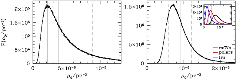
Figure 3: The $\rho$ distributions for non-magnetic CVs (left-hand panel) and mCVs (right-hand panel) resulting from our simulations. Solid lines in both panels mark the modes, medians, and means of the distributions; dashed lines show 1-$\sigma$ intervals. The probability distribution functions shown in the inset are for the whole mCV sample, polars alone (red), and IPs alone (blue). Reproduced from Pretorius & Knigge (2012) and Pretorius, Knigge & Schwope (2013).

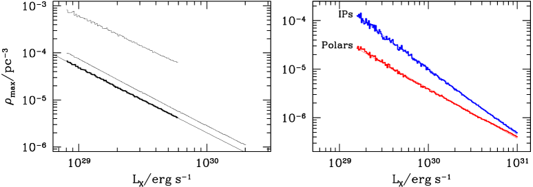
Figure 4: The upper limit on $\rho$ as a function of X-ray luminosity for undetected populations of CVs. The left-hand panel is for non-magnetic CVs, and the right-hand panel for IPs (blue) and polars (red). In the left-hand panel, the 2 upper, fine histograms show the corresponding results for the RBS (middle) and NEP (top) surveys alone. Note that the assumed X-ray spectra of non-magnetic CVs, polars, and IPs are different, hence the different slopes. Reproduced from Pretorius & Knigge (2012) and Pretorius et al. (2013).

4 Discussion

4.1 Missing non-magnetic CVs

We discuss our measured $\rho_{n-m}$, as well as the upper limit, in the context of the predicted (i) large total space density of non-magnetic CVs, and (ii) large predicted fraction of normal short-period CVs and period bouncers.

Population synthesis models predict that at most a few percent of all CVs are above the period gap (Kolb 1993 finds less than 1%, while Knigge et al. 2011 predict 3%). Although we find that long-period systems account for slightly more than 50% of our total $\rho_{n-m}$, the data do not rule out these theoretical predictions. For example, using the Knigge et al. (2011) fraction of long-period systems, and assuming that we have not significantly under-estimated the space density of long-period CVs, the space density of short-period CVs is $\simeq 2\times 10^{-6}\,\mathrm{pc^{-3}}(97/3)\simeq 6\times 10^{-5}\,\mathrm{pc^{-3}}$. Using the upper limit on $\rho_{n-m}$ from Section 3.3.2, we find that a short-period CV population of this size could escape detection in the two surveys, provided that the systems have $L_{X}\raisebox{-2.58334pt}{$\,\stackrel{{\scriptstyle\raisebox{-0.60275pt}{$\textstyle<$}}}{{\sim}}\,$}8\times 10^{28}\,\mathrm{erg\,s^{-1}}$ (for the simple case of a hypothetical single-$L_{X}$ population of faint, undetected CVs). To reach the predicted $\rho=2\times 10^{-4}\,\mathrm{pc^{-3}}$ would require that the majority of CVs has X-ray luminosities below $L_{X}=4\times 10^{28}\,\mathrm{erg\,s^{-1}}$.

4.2 Evolutionary relationship between IPs and polars

If one assumes that long-period IPs are the sole progenitors of short-period polars, and that all IPs synchronize once they have crossed the period gap, then the ratio of the space densities of long-$P_{orb}$ IPs and short-$P_{orb}$ polars ($\rho_{IP,lp}$ and $\rho_{polar,sp}$) should simply reflect their relative evolutionary time-scales. The observed logarithm of this ratio is $\log{(\rho_{polar,sp}/\rho_{IP,lp})}=0.32\pm 0.36$. If the evolution of long-period IPs is driven by MB, while that of short-period polars is driven solely by GR, the evolutionary time-scale of short-period polars should be $\raisebox{-2.58334pt}{$\,\stackrel{{\scriptstyle\raisebox{-0.60275pt}{$\textstyle>$}}}{{\sim}}\,$}5\times$ that of long-period IPs (e.g. Knigge et al. 2011). This is completely consistent with the ratio of the inferred space densities. In fact, at 2-$\sigma$, the uncertainties are large enough to encompass both ratios exceeding 10 and ratios less than unity. This means that, with the currently available space density estimates for polars and IPs, we cannot place strong constraints on the evolutionary relationship between the two classes. Nevertheless, it is interesting to note that the simplest possible model, in which short-period polars derive from long-period IPs, is not ruled out by their observed space densities.

4.3 Intrinsic fraction of mCVs

Combining the space density estimates of magnetic and non-magnetic CVs to estimate the intrinsic fraction of mCVs, we find $\log(f_{mCV})=-0.80^{+0.27}_{-0.36}$. This is consistent, within the considerable uncertainties, with the fraction of isolated WDs that are strongly magnetic . In fact, it seems likely that the X-ray-selected CV sample is more complete for mCVs than it is for non-magnetic CVs. Therefore, the incidence of magnetism is not obviously enhanced amongst CV primaries compared to isolated WDs.

4.4 Galactic X-ray Source Populations

We consider if it is plausible that IPs dominate X-ray source populations above $L_{X}\simeq 10^{31}{\rm ergs^{-1}}$, taking the Galactic Centre as an example. The deep Chandra survey of Muno et al. (2009) includes $\simeq 9000$ sources down to $L_{X}\simeq 10^{31}\,{\rm ergs^{-1}}$, in an area of $\simeq 10^{-3}{\rm deg^{2}}$. Approximating the volume covered by the survey as a sphere of radius $150$ pc, the space density of X-ray sources in the Galactic Centre is $\rho_{X,GC}\sim 6\times 10^{-4}\,{\rm pc^{-3}}$, while the local space density of IPs is $\rho_{IP}\sim 3\times 10^{-7}\,{\rm pc^{-3}}$. However, the stellar space density in the Galactic centre is $\simeq 1600\times$ higher than in the solar neighborhood. Thus these densities are consistent, and we conclude that IPs remain a viable explanation for most of the X-ray sources seen in the Galactic Centre.

5 Conclusions

With the assumption that the CV samples from the RBS and NEP surveys are representative of the intrinsic populations (in the sense that we detected at least one system at the faintest ends of the luminosity functions of those populations), we find $\rho_{n-m}=4^{+6}_{-2}\times 10^{-6}\,\mathrm{pc^{-3}}$ and $\rho_{mCV}=8^{+4}_{-2}\times 10^{-7}\,\mathrm{pc^{-3}}$ ($\rho_{polar}=5^{+3}_{-2}\times 10^{-7}\,\mathrm{pc^{-3}}$ and $\rho_{IP}=3^{+2}_{-1}\times 10^{-7}\,\mathrm{pc^{-3}}$).

The data are consistent with more than half of non-magnetic CVs having $28.7<\mathrm{log}(L_{X}/\mathrm{erg\,s^{-1}})<29.7$, and escaping detection. However, to reach $\rho_{n-m}=2\times 10^{-4}\,\mathrm{pc^{-3}}$ (at the high end of the predicted range), we require that the majority of non-magnetic CVs have $L_{X}\raisebox{-2.58334pt}{$\,\stackrel{{\scriptstyle\raisebox{-0.60275pt}{$\textstyle<$}}}{{\sim}}\,$}4\times 10^{28}\,\mathrm{erg\,s^{-1}}$.

The ratio of the space density of short-period polars to long-period IPs is consistent with the very simple hypothesis that long-period IPs evolve into short-period polars, and that this accounts for the whole population of short-period polars.

Existing data cannot rule out that strongly magnetic WDs have the same incidence amongst CVs as in the field.

When the local space density of IPs is scaled to the density of stars in the Galactic Centre, it is sufficiently high to account for the number of bright X-ray sources detected in that region.

I thank the organizes for a successful meeting, and for inviting me to present this review.

References

- [1] Chanmugam G., Ray A.: 1984, ApJ, 285, 252
- [2] Cumming A.: 2002, MNRAS, 333, 589
- [3] de Kool M.: 1992, A&A, 261, 188
- [4] Gänsicke B. T., et al.: 2009, MNRAS, 397, 2170
- [5] Henry J.P., et al.: 2006, ApJS, 162, 304
- [6] Knigge C.: 2006, MNRAS, 373, 484
- [7] Knigge C., Baraffe I., Patterson J.: 2011, ApJS, 194, 28
- [8] Kolb U.: 1993, A&A, 271, 149
- [9] Külebi B., et al.: 2009, A&A, 506, 1341
- [10] Li J., Wickramasinghe D. T.: 1998, MNRAS, 300, 718
- [11] Muno M. P., et al.: 2009, ApJS, 181, 110
- [12] Patterson J.: 1984, ApJS, 54, 443
- [13] Patterson J.: 1994, PASP, 106, 209
- [14] Patterson J.: 1998, PASP, 110, 1132
- [15] Patterson J.: 2011, MNRAS, 411,2695
- [16] Pretorius M. L., Knigge C.: 2012, MNRAS, 419, 1442
- [17] Pretorius M. L., Knigge C.: 2008a, MNRAS, 385, 1471
- [18] Pretorius M. L., Knigge C.: 2008b, MNRAS, 385, 1485
- [19] Pretorius M. L., Knigge C., Kolb U.: 2007a, MNRAS, 374, 1495
- [20] Pretorius, M. L., Knigge, C., Schwope, A. D.: 2013, MNRAS, 432, 570
- [21] Pretorius M. L., et al.: 2007b, MNRAS, 382, 1279
- [22] Ritter H., Kolb U.: 2003, A&A, 404, 301
- [23] Schwope A.D., et al.: 2002, A&A, 396, 895
- [24] Tout C. A., et al.: 2008, MNRAS, 387, 897
- [25] Townsley D. M., Gänsicke B. T.: 2009, ApJ, 693, 1007
- [26] Wickramasinghe D. T., Wu K., Ferrario L.: 1991, MNRAS, 249, 460
- [27] Warner B.: 1987, MNRAS, 227, 23
- [28] van Teeseling A., Beuermann K., Verbunt F.: 1996, A&A, 315, 467